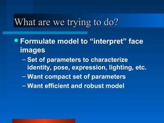
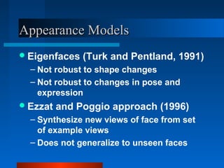
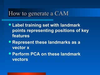
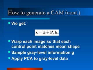
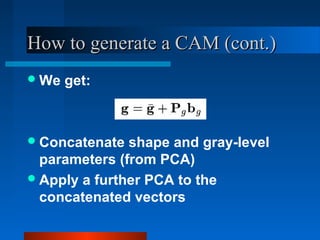
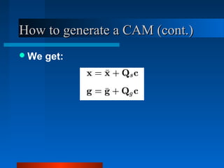
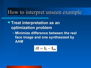
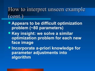
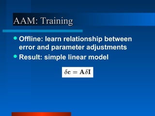
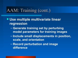
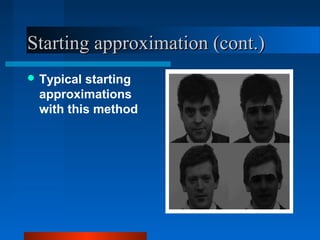
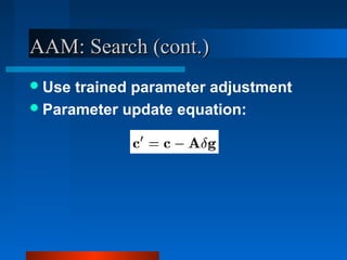
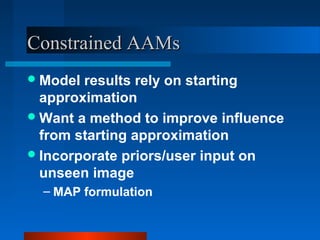
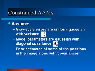
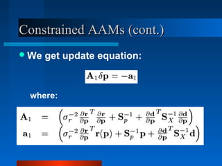
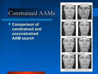
Active Appearance Models (AAMs) combine shape and texture models into a single statistical model. AAMs are trained on labeled images to learn the relationship between shape, texture, and model parameters. To interpret a new image, an optimization problem is solved to minimize the difference between the image and one synthesized by the AAM. The model parameters are updated iteratively based on a linear model trained to relate parameter adjustments to image differences. Constrained AAMs incorporate prior information to improve the influence of the starting approximation on the search results.

1. Active Appearance Models
Edwards, Taylor, and Cootes
Presented by Bryan Russell

2. Overview
 Overview of Appearance Models
 Combined Appearance Models
 Active Appearance Model Search
 Results
 Constrained Active Appearance
Models

3. What are we trying to do?
 Formulate model to “interpret” face
images
– Set of parameters to characterize
identity, pose, expression, lighting, etc.
– Want compact set of parameters
– Want efficient and robust model

4. Appearance Models
 Eigenfaces (Turk and Pentland, 1991)
– Not robust to shape changes
– Not robust to changes in pose and
expression
 Ezzat and Poggio approach (1996)
– Synthesize new views of face from set
of example views
– Does not generalize to unseen faces

5. First approach: Active Shape
Model (ASM)
 Point Distribution Model

6. First Approach: ASM (cont.)
 Training: Apply PCA to labeled
images
 New image
– Project mean shape
– Iteratively modify model points to fit
local neighborhood

7. Lessons learned
 ASM is relatively fast
 ASM too simplistic; not robust when
new images are introduced
 May not converge to good solution
 Key insight: ASM does not
incorporate all gray-level information
in parameters

8. Combined Appearance Models
 Combine shape and gray-level
variation in single statistical
appearance model
 Goals:
– Model has better representational power
– Model inherits appearance models
benefits
– Model has comparable performance

9. How to generate a CAM
 Label training set with landmark
points representing positions of key
features
 Represent these landmarks as a
vector x
 Perform PCA on these landmark
vectors

10. How to generate a CAM (cont.)
 We get:
 Warp each image so that each
control point matches mean shape
 Sample gray-level information g
 Apply PCA to gray-level data

11. How to generate a CAM (cont.)
 We get:
 Concatenate shape and gray-level
parameters (from PCA)
 Apply a further PCA to the
concatenated vectors

12. How to generate a CAM (cont.)
 We get:

13. CAM Properties
 Combines shape and gray-level
variations in one model
– No need for separate models
 Compared to separate models, in
general, needs fewer parameters
 Uses all available information

14. CAM Properties (cont.)
 Inherits appearance model benefits
– Able to represent any face within
bounds of the training set
– Robust interpretation
 Model parameters characterize facial
features

15. CAM Properties (cont.)
 Obtainparameters for inter and intra
class variation (identity and residual
parameters) – “explains” face

16. CAM Properties (cont.)
 Useful for tracking and identification
– Refer to: G.J.Edwards, C.J.Taylor, T.F.Cootes. "Learning
to Identify and Track Faces in Image Sequences“. Int.
Conf. on Face and Gesture Recognition, p. 260-265,
1998.
 Note:shape and gray-level variations
are correlated

17. How to interpret unseen example
 Treat
interpretation as an
optimization problem
– Minimize difference between the real
face image and one synthesized by
AAM

18. How to interpret unseen example
(cont.)
 Appears to be difficult optimization
problem (~80 parameters)
 Key insight: we solve a similar
optimization problem for each new
face image
 Incorporate a-priori knowledge for
parameter adjustments into
algorithm

19. AAM: Training
 Offline:learn relationship between
error and parameter adjustments
 Result: simple linear model

20. AAM: Training (cont.)
 Usemultiple multivariate linear
regression
– Generate training set by perturbing
model parameters for training images
– Include small displacements in position,
scale, and orientation
– Record perturbation and image
difference

21. AAM: Training (cont.)
 Important to consider frame of
reference when computing image
difference
– Use shape-normalized representation
(warping)
– Calculate image difference using gray
level vectors:

22. AAM: Training (cont.)
 Updated linear relationship:
 Want a model that holds over large
error range
 Experimentally, optimal perturbation
around 0.5 standard deviations for
each parameter

23. AAM: Search
 Begin with reasonable starting
approximation for face
 Want approximation to be fast and
simple
 Perhaps Viola’s method can be
applied here

24. Starting approximation
 Subsample model and image
 Use simple eigenface metric:

25. Starting approximation (cont.)
 Typicalstarting
approximations
with this method

26. AAM: Search (cont.)
 Use trained parameter adjustment
 Parameter update equation:

27. Experimental results
 Training:
– 400 images, 112
landmark points
– 80 CAM parameters
– Parameters explain
98% observed
variation
 Testing:
– 80 previously
unseen faces

28. Experimental results (cont.)
 Search results
after initial, 2, 5,
and 12 iterations

29. Experimental results (cont.)
 Search
convergence:
– Gray-level sample
error vs. number of
iterations

30. Experimental results (cont.)
 More reconstructions:

31. Experimental results (cont.)

32. Experimental results (cont.)
 Knee images:
– Training: 30 examples, 42 landmarks

33. Experimental results (cont.)
 Search results after initial, 2
iterations, and convergence:

34. Constrained AAMs
 Model results rely on starting
approximation
 Want a method to improve influence
from starting approximation
 Incorporate priors/user input on
unseen image
– MAP formulation

35. Constrained AAMs
 Assume:
– Gray-scale errors are uniform gaussian
with variance
– Model parameters are gaussian with
diagonal covariance
– Prior estimates of some of the positions
in the image along with covariances

36. Constrained AAMs (cont.)
 We get update equation:
where:

37. Constrained AAMs
 Comparison of
constrained and
unconstrained
AAM search

38. Conclusions
 Combined Appearance Models
provide an effective means to
separate identity and intra-class
variation
– Can be used for tracking and face
classification
 ActiveAppearance Models enables
us to effectively and efficiently
update the model parameters

39. Conclusions (cont.)
 Approach dependent on starting
approximation
 Cannot directly handle cases well
outside of the training set (e.g.
occlusions, extremely deformable
objects)