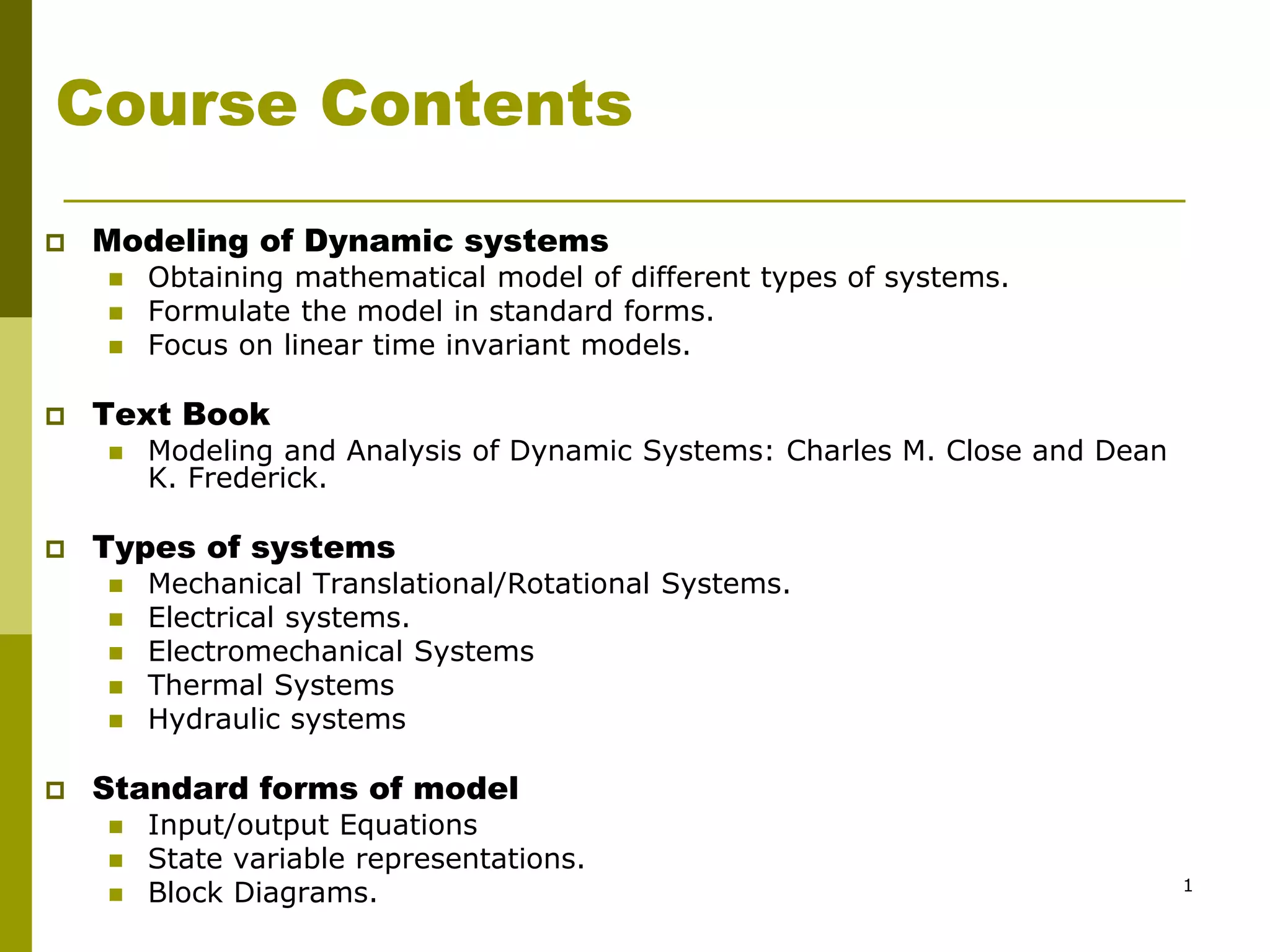
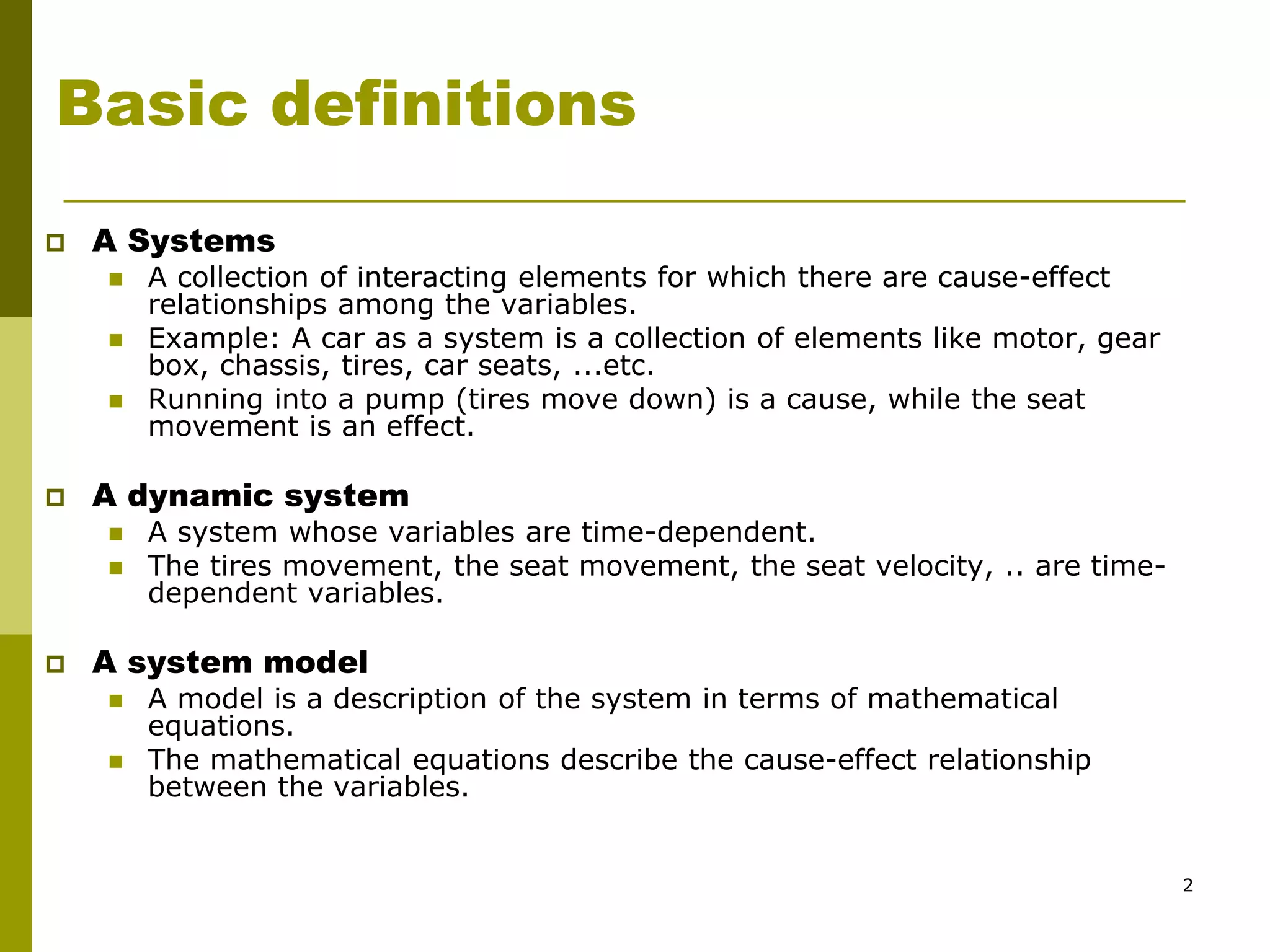
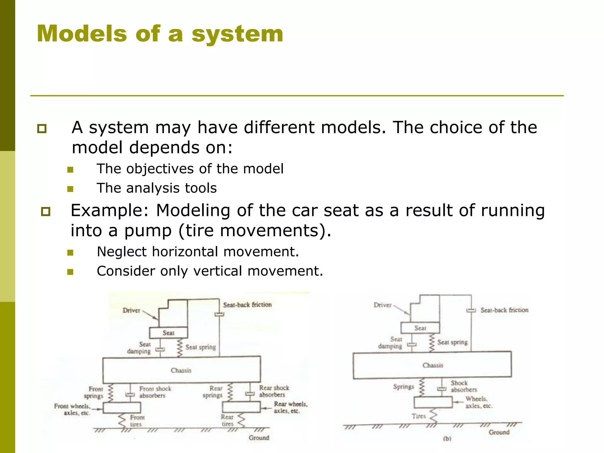
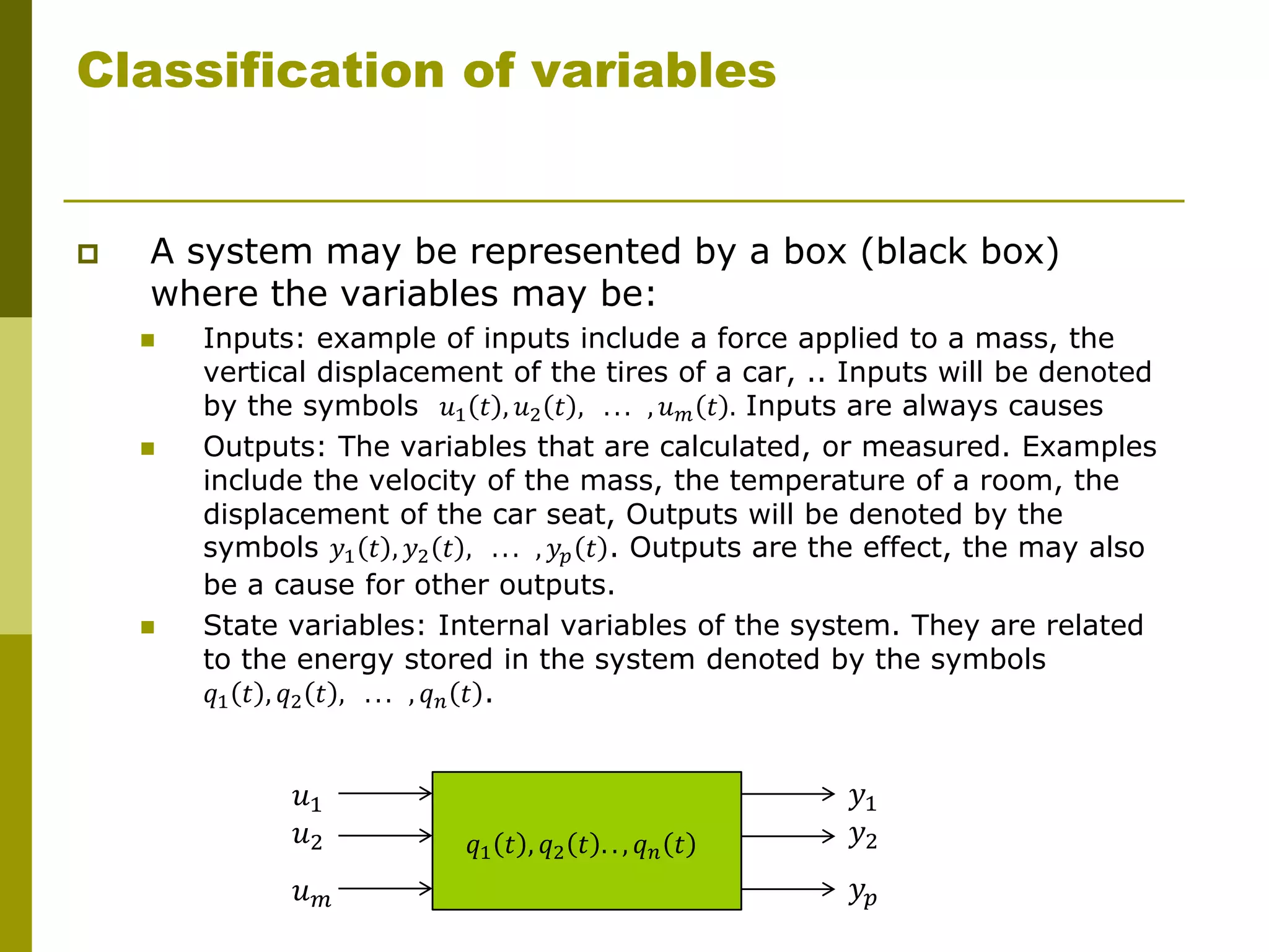
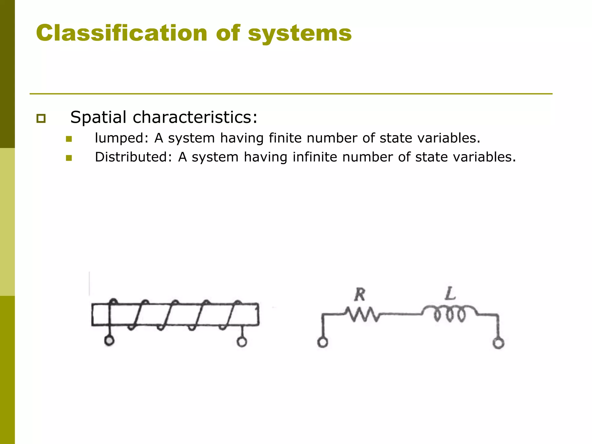
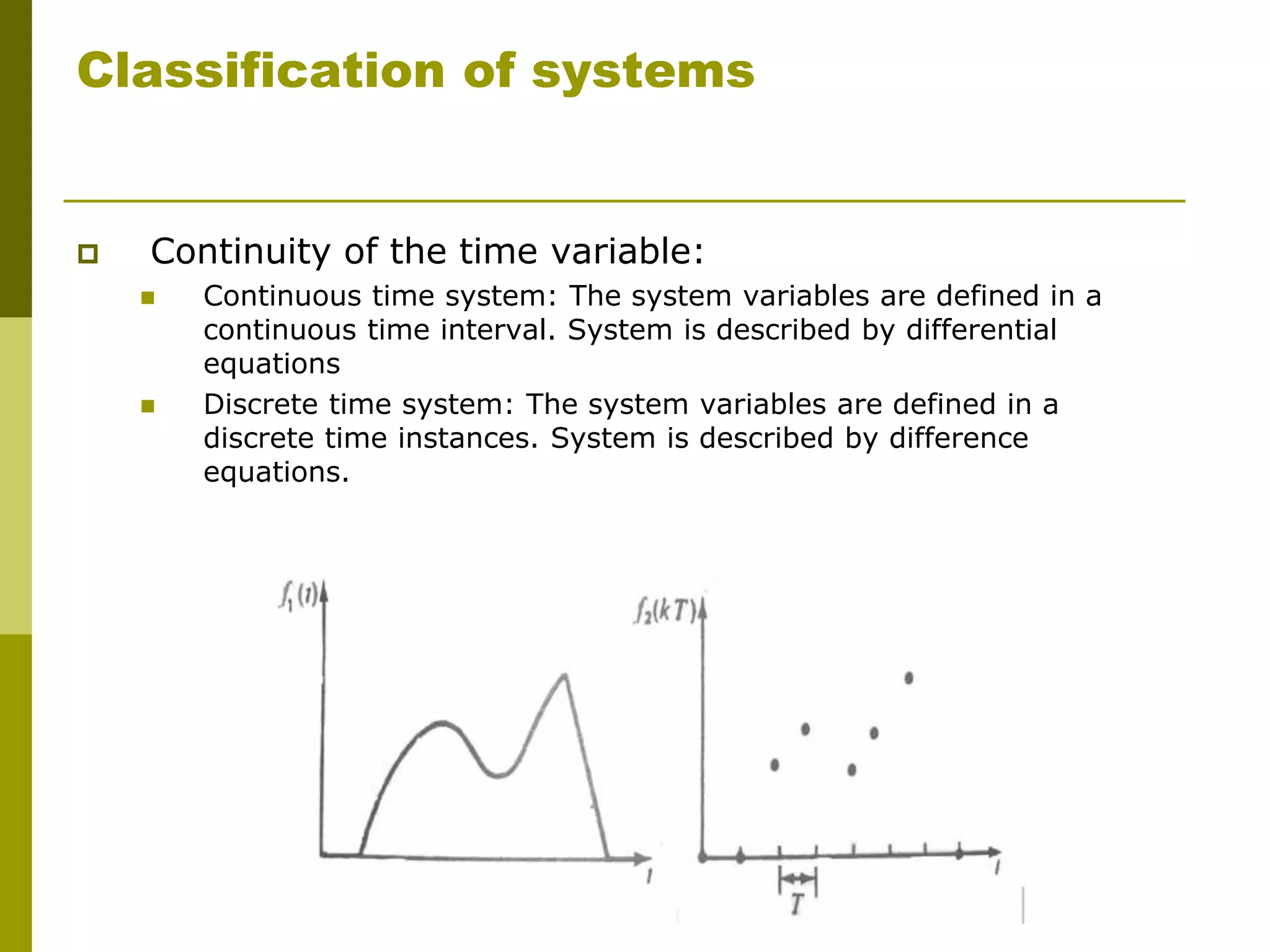
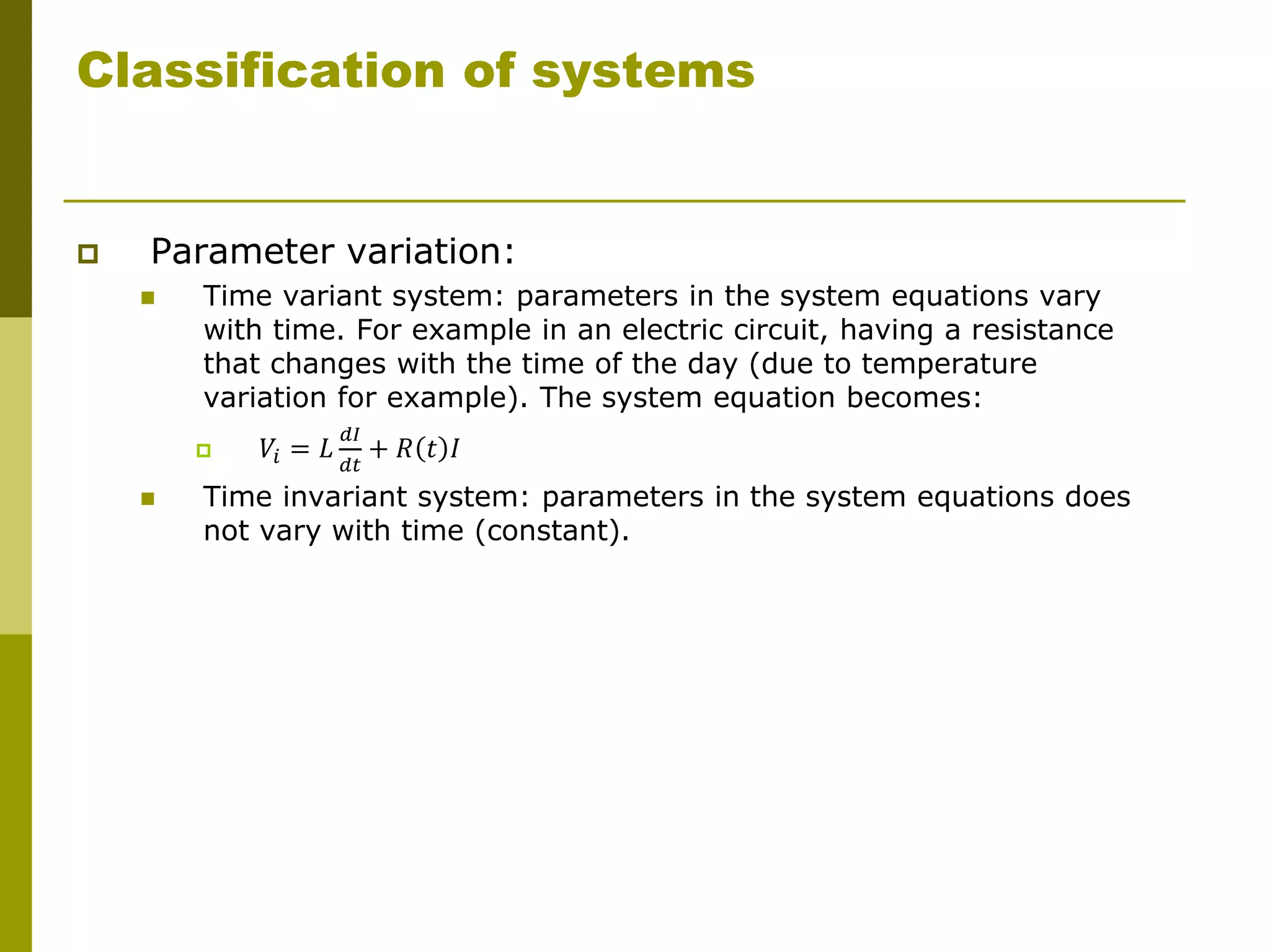
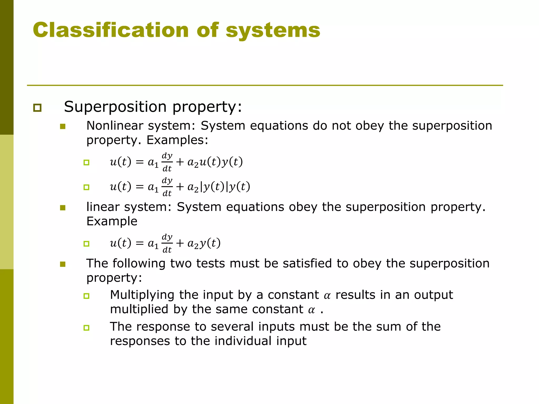
This document provides an overview of modeling dynamic systems. It discusses obtaining mathematical models of different types of systems like mechanical, electrical, and thermal systems. The models can be represented using input/output equations, state variable representations, or block diagrams. The document also defines key terms like dynamic systems, system models, inputs, outputs, and state variables. It classifies systems based on characteristics such as being lumped or distributed, continuous or discrete time, time variant or invariant, and linear or nonlinear.

1. 1
Course Contents
 Modeling of Dynamic systems
 Obtaining mathematical model of different types of systems.
 Formulate the model in standard forms.
 Focus on linear time invariant models.
 Text Book
 Modeling and Analysis of Dynamic Systems: Charles M. Close and Dean
K. Frederick.
 Types of systems
 Mechanical Translational/Rotational Systems.
 Electrical systems.
 Electromechanical Systems
 Thermal Systems
 Hydraulic systems
 Standard forms of model
 Input/output Equations
 State variable representations.
 Block Diagrams.

2. 2
Basic definitions
 A Systems
 A collection of interacting elements for which there are cause-effect
relationships among the variables.
 Example: A car as a system is a collection of elements like motor, gear
box, chassis, tires, car seats, ...etc.
 Running into a pump (tires move down) is a cause, while the seat
movement is an effect.
 A dynamic system
 A system whose variables are time-dependent.
 The tires movement, the seat movement, the seat velocity, .. are time-
dependent variables.
 A system model
 A model is a description of the system in terms of mathematical
equations.
 The mathematical equations describe the cause-effect relationship
between the variables.

3. Models of a system
 A system may have different models. The choice of the
model depends on:
 The objectives of the model
 The analysis tools
 Example: Modeling of the car seat as a result of running
into a pump (tire movements).
 Neglect horizontal movement.
 Consider only vertical movement.

4. Classification of variables
 A system may be represented by a box (black box)
where the variables may be:
 Inputs: example of inputs include a force applied to a mass, the
vertical displacement of the tires of a car, .. Inputs will be denoted
by the symbols 𝑢1 𝑡 , 𝑢2 𝑡 , . . . , 𝑢𝑚 𝑡 . Inputs are always causes
 Outputs: The variables that are calculated, or measured. Examples
include the velocity of the mass, the temperature of a room, the
displacement of the car seat, Outputs will be denoted by the
symbols 𝑦1 𝑡 , 𝑦2 𝑡 , . . . , 𝑦𝑝 𝑡 . Outputs are the effect, the may also
be a cause for other outputs.
 State variables: Internal variables of the system. They are related
to the energy stored in the system denoted by the symbols
𝑞1 𝑡 , 𝑞2 𝑡 , . . . , 𝑞𝑛 𝑡 .
𝑢1
𝑢2
𝑢𝑚
𝑦1
𝑦2
𝑦𝑝
𝑞1 𝑡 , 𝑞2 𝑡 . . , 𝑞𝑛 𝑡

5. Classification of systems
 Spatial characteristics:
 lumped: A system having finite number of state variables.
 Distributed: A system having infinite number of state variables.

6. Classification of systems
 Continuity of the time variable:
 Continuous time system: The system variables are defined in a
continuous time interval. System is described by differential
equations
 Discrete time system: The system variables are defined in a
discrete time instances. System is described by difference
equations.

7. Classification of systems
 Parameter variation:
 Time variant system: parameters in the system equations vary
with time. For example in an electric circuit, having a resistance
that changes with the time of the day (due to temperature
variation for example). The system equation becomes:
 𝑉𝑖 = 𝐿
𝑑𝐼
𝑑𝑡
+ 𝑅 𝑡 𝐼
 Time invariant system: parameters in the system equations does
not vary with time (constant).

8. Classification of systems
 Superposition property:
 Nonlinear system: System equations do not obey the superposition
property. Examples:
 𝑢 𝑡 = 𝑎1
𝑑𝑦
𝑑𝑡
+ 𝑎2𝑢 𝑡 𝑦 𝑡
 𝑢 𝑡 = 𝑎1
𝑑𝑦
𝑑𝑡
+ 𝑎2 𝑦 𝑡 𝑦 𝑡
 linear system: System equations obey the superposition property.
Example
 𝑢 𝑡 = 𝑎1
𝑑𝑦
𝑑𝑡
+ 𝑎2𝑦 𝑡
 The following two tests must be satisfied to obey the superposition
property:
 Multiplying the input by a constant 𝛼 results in an output
multiplied by the same constant 𝛼 .
 The response to several inputs must be the sum of the
responses to the individual input