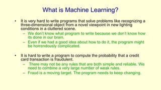
Neural Networks for Machine Learning

            Lecture 1a
 Why do we need machine learning?

 Geoffrey Hinton
 with
 Nitish Srivastava
 Kevin Swersky
What is Machine Learning?
•   It is very hard to write programs that solve problems like recognizing a
    three-dimensional object from a novel viewpoint in new lighting
    conditions in a cluttered scene.
      – We don’t know what program to write because we don’t know how
          its done in our brain.
      – Even if we had a good idea about how to do it, the program might
          be horrendously complicated.

•   It is hard to write a program to compute the probability that a credit
    card transaction is fraudulent.
      – There may not be any rules that are both simple and reliable. We
          need to combine a very large number of weak rules.
      – Fraud is a moving target. The program needs to keep changing.
The Machine Learning Approach
• Instead of writing a program by hand for each specific task, we collect
  lots of examples that specify the correct output for a given input.
• A machine learning algorithm then takes these examples and produces
  a program that does the job.
   – The program produced by the learning algorithm may look very
      different from a typical hand-written program. It may contain millions
      of numbers.
   – If we do it right, the program works for new cases as well as the ones
      we trained it on.
   – If the data changes the program can change too by training on the
      new data.
• Massive amounts of computation are now cheaper than paying
  someone to write a task-specific program.
Some examples of tasks best solved by learning
• Recognizing patterns:
   – Objects in real scenes
   – Facial identities or facial expressions
   – Spoken words
• Recognizing anomalies:
   – Unusual sequences of credit card transactions
   – Unusual patterns of sensor readings in a nuclear power plant
• Prediction:
   – Future stock prices or currency exchange rates
   – Which movies will a person like?
A standard example of machine learning
• A lot of genetics is done on fruit flies.
   – They are convenient because they breed fast.
   – We already know a lot about them.
• The MNIST database of hand-written digits is the the machine learning
  equivalent of fruit flies.
   – They are publicly available and we can learn them quite fast in a
      moderate-sized neural net.
   – We know a huge amount about how well various machine learning
      methods do on MNIST.
• We will use MNIST as our standard task.
It is very hard to say what makes a 2
Beyond MNIST: The ImageNet task
• 1000 different object classes in 1.3 million high-resolution training images
  from the web.
    – Best system in 2010 competition got 47% error for its first choice and
      25% error for its top 5 choices.
• Jitendra Malik (an eminent neural net sceptic) said that this competition is
  a good test of whether deep neural networks work well for object
  recognition.
    – A very deep neural net (Krizhevsky et. al. 2012) gets less that 40%
      error for its first choice and less than 20% for its top 5 choices
      (see lecture 5).
Some examples from an earlier version of the net
It can deal with a wide range of objects
It makes some really cool errors
The Speech Recognition Task
• A speech recognition system has several stages:
   – Pre-processing: Convert the sound wave into a vector of acoustic
     coefficients. Extract a new vector about every 10 mille seconds.
   – The acoustic model: Use a few adjacent vectors of acoustic coefficients
     to place bets on which part of which phoneme is being spoken.
   – Decoding: Find the sequence of bets that does the best job of fitting the
     acoustic data and also fitting a model of the kinds of things people say.
• Deep neural networks pioneered by George Dahl and Abdel-rahman
  Mohamed are now replacing the previous machine learning method
  for the acoustic model.
Phone recognition on the TIMIT benchmark
                       (Mohamed, Dahl, & Hinton, 2012)
        183 HMM-state labels           – After standard post-processing
    not pre-trained                      using a bi-phone model, a deep
       2000 logistic hidden units        net with 8 layers gets 20.7% error
5 more layers of                         rate.
pre-trained weights                    – The best previous speaker-
       2000 logistic hidden units        independent result on TIMIT was
                                         24.4% and this required averaging
       2000 logistic hidden units        several models.
                                       – Li Deng (at MSR) realised that this
  15 frames of 40 filterbank outputs     result could change the way
  + their temporal derivatives           speech recognition was done.
Word error rates from MSR, IBM, & Google
(Hinton et. al. IEEE Signal Processing Magazine, Nov 2012)

The task            Hours of        Deep neural     Gaussian   GMM with
                    training data   network         Mixture    more data
                                                    Model

Switchboard         309             18.5%           27.4%      18.6%
(Microsoft                                                     (2000 hrs)
Research)
English broadcast   50              17.5%           18.8%
news (IBM)

Google voice        5,870           12.3%                      16.0%
search                              (and falling)              (>>5,870 hrs)
(android 4.1)
Neural Networks for Machine Learning

               Lecture 1b
        What are neural networks?

 Geoffrey Hinton
 with
 Nitish Srivastava
 Kevin Swersky
Reasons to study neural computation
•   To understand how the brain actually works.
     – Its very big and very complicated and made of stuff that dies when you
        poke it around. So we need to use computer simulations.
•   To understand a style of parallel computation inspired by neurons and their
    adaptive connections.
     – Very different style from sequential computation.
          • should be good for things that brains are good at (e.g. vision)
          • Should be bad for things that brains are bad at (e.g. 23 x 71)
•   To solve practical problems by using novel learning algorithms inspired by
    the brain (this course)
     – Learning algorithms can be very useful even if they are not how the
       brain actually works.
A typical cortical neuron
•   Gross physical structure:
     – There is one axon that branches
     – There is a dendritic tree that collects input from
       other neurons.
                                                                    axon
•   Axons typically contact dendritic trees at synapses
     – A spike of activity in the axon causes charge to be
       injected into the post-synaptic neuron.                         axon hillock
                                                             body
•   Spike generation:                                                      dendritic
     – There is an axon hillock that generates outgoing                    tree
        spikes whenever enough charge has flowed in at
        synapses to depolarize the cell membrane.
Synapses

• When a spike of activity travels along an axon and
  arrives at a synapse it causes vesicles of transmitter
  chemical to be released.
   – There are several kinds of transmitter.

• The transmitter molecules diffuse across the synaptic
  cleft and bind to receptor molecules in the membrane of
  the post-synaptic neuron thus changing their shape.
   – This opens up holes that allow specific ions in or
      out.
How synapses adapt

• The effectiveness of the synapse can be changed:
   – vary the number of vesicles of transmitter.
   – vary the number of receptor molecules.

• Synapses are slow, but they have advantages over RAM
   – They are very small and very low-power.
   – They adapt using locally available signals
      • But what rules do they use to decide how to change?
How the brain works on one slide!
•   Each neuron receives inputs from other neurons
     - A few neurons also connect to receptors.
     - Cortical neurons use spikes to communicate.
•   The effect of each input line on the neuron is controlled
    by a synaptic weight
     – The weights can be positive or negative.
•   The synaptic weights adapt so that the whole network learns to perform
    useful computations
     – Recognizing objects, understanding language, making plans,
        controlling the body.
                         11                             4
•   You have about 10 neurons each with about 10 weights.
     – A huge number of weights can affect the computation in a very short
        time. Much better bandwidth than a workstation.
Modularity and the brain
•   Different bits of the cortex do different things.
     – Local damage to the brain has specific effects.
     – Specific tasks increase the blood flow to specific regions.
•   But cortex looks pretty much the same all over.
     – Early brain damage makes functions relocate.
•   Cortex is made of general purpose stuff that has the ability to turn into
    special purpose hardware in response to experience.
     – This gives rapid parallel computation plus flexibility.
     – Conventional computers get flexibility by having stored sequential
        programs, but this requires very fast central processors to perform
        long sequential computations.
Neural Networks for Machine Learning

           Lecture 1c
  Some simple models of neurons

  Geoffrey Hinton
  with
  Nitish Srivastava
  Kevin Swersky
Idealized neurons
•   To model things we have to idealize them (e.g. atoms)
      – Idealization removes complicated details that are not essential
          for understanding the main principles.
      – It allows us to apply mathematics and to make analogies to
          other, familiar systems.
      – Once we understand the basic principles, its easy to add
          complexity to make the model more faithful.
•   It is often worth understanding models that are known to be wrong
    (but we must not forget that they are wrong!)
      – E.g. neurons that communicate real values rather than discrete
          spikes of activity.
Linear neurons
• These are simple but computationally limited
   – If we can make them learn we may get insight into more
     complicated neurons.
         bias         i th input


  y b                   xi wi
                  i                weight on
output
         index over                i th input
         input connections
Linear neurons
• These are simple but computationally limited
   – If we can make them learn we may get insight into more
     complicated neurons.


   y b              xi wi            y
                                       0
                i
                                               0
                                                   b       xi wi
                                                       i
Binary threshold neurons
• McCulloch-Pitts (1943): influenced Von Neumann.
   – First compute a weighted sum of the inputs.
   – Then send out a fixed size spike of activity if
     the weighted sum exceeds a threshold.                 1
   – McCulloch and Pitts thought that each spike


                                                       output
     is like the truth value of a proposition and
     each neuron combines truth values to
     compute the truth value of another                         0
     proposition!                                                    threshold
                                                                    weighted input
Binary threshold neurons

• There are two equivalent ways to write the equations for
  a binary threshold neuron:

 z          xi wi                        z = b + å xi wi
                              q = -b
       i                                            i

           1 if   z                              1 if   z³0
 y                                       y
           0 otherwise                           0 otherwise
Rectified Linear Neurons
      (sometimes called linear threshold neurons)

They compute a linear weighted sum of their inputs.
The output is a non-linear function of the total input.


z = b + å xi wi
            i
        z if z >0
y =
                                 y
       0 otherwise                                 0      z
Sigmoid neurons

                                z = b + å xi wi
• These give a real-valued                               1
                                                  y=
                                                           -z
  output that is a smooth and
  bounded function of their
  total input.
                                           i           1+ e
   – Typically they use the
      logistic function                1
   – They have nice
      derivatives which make     y   0.5
      learning easy (see
      lecture 3).                      0
                                                   0     z
Stochastic binary neurons
• These use the same equations      z = b + å xi wi   p(s = 1) =
                                                                     1
  as logistic units.                                               1+ e
                                                                         -z
                                              i
   – But they treat the output of
      the logistic as the
      probability of producing a          1
      spike in a short time
      window.                       p 0.5
• We can do a similar trick for
  rectified linear units:                 0
   – The output is treated as the                       0
      Poisson rate for spikes.                        z
Neural Networks for Machine Learning

              Lecture 1d
     A simple example of learning

  Geoffrey Hinton
  with
  Nitish Srivastava
  Kevin Swersky
A very simple way to recognize handwritten shapes
• Consider a neural network with two
  layers of neurons.
                                            0 1 2 3 4 5 6 7 8 9
   – neurons in the top layer represent
      known shapes.
   – neurons in the bottom layer
      represent pixel intensities.
• A pixel gets to vote if it has ink on it.
   – Each inked pixel can vote for several
      different shapes.
• The shape that gets the most votes wins.
How to display the weights
   1      2       3       4       5       6       7       8       9      0


                                               The input
                                               image

Give each output unit its own “map” of the input image and display the weight
coming from each pixel in the location of that pixel in the map.
Use a black or white blob with the area representing the magnitude of the weight
and the color representing the sign.
How to learn the weights
1      2       3       4       5      6       7       8       9       0


                                           The image


Show the network an image and increment the weights from active pixels
to the correct class.
Then decrement the weights from active pixels to whatever class the
network guesses.
1   2   3   4   5     6     7   8   9   0


                The image
1   2   3   4   5     6     7   8   9   0


                The image
1   2   3   4   5     6     7   8   9   0


                The image
1   2   3   4   5     6     7   8   9   0


                The image
1   2   3   4   5     6     7   8   9   0


                The image
The learned weights
 1      2       3      4       5      6       7      8       9      0


                              The image
The details of the learning algorithm will be explained in future lectures.
Why the simple learning algorithm is insufficient

 • A two layer network with a single winner in the top layer is
   equivalent to having a rigid template for each shape.
    – The winner is the template that has the biggest overlap
       with the ink.
 • The ways in which hand-written digits vary are much too
   complicated to be captured by simple template matches of
   whole shapes.
    – To capture all the allowable variations of a digit we need
       to learn the features that it is composed of.
Examples of handwritten digits that can be recognized
       correctly the first time they are seen
Neural Networks for Machine Learning

              Lecture 1e
         Three types of learning

Geoffrey Hinton
with
Nitish Srivastava
Kevin Swersky
Types of learning task
• Supervised learning
   – Learn to predict an output when given an input vector.

• Reinforcement learning
   – Learn to select an action to maximize payoff.

• Unsupervised learning
   – Discover a good internal representation of the input.
Two types of supervised learning

• Each training case consists of an input vector x and a target output t.

• Regression: The target output is a real number or a whole vector of
  real numbers.
   – The price of a stock in 6 months time.
   – The temperature at noon tomorrow.

• Classification: The target output is a class label.
   – The simplest case is a choice between 1 and 0.
   – We can also have multiple alternative labels.
How supervised learning typically works
• We start by choosing a model-class: y = f (x;W)
  – A model-class, f, is a way of using some numerical
    parameters, W, to map each input vector, x, into a predicted
    output y.

• Learning usually means adjusting the parameters to reduce the
  discrepancy between the target output, t, on each training case
  and the actual output, y, produced by the model.
                     1
   – For regression, 2 (y - t)2 is often a sensible measure of the
     discrepancy.
   – For classification there are other measures that are generally
     more sensible (they also work better).
Reinforcement learning
• In reinforcement learning, the output is an action or sequence of actions
  and the only supervisory signal is an occasional scalar reward.
   – The goal in selecting each action is to maximize the expected sum
      of the future rewards.
   – We usually use a discount factor for delayed rewards so that we
      don’t have to look too far into the future.
• Reinforcement learning is difficult:
   – The rewards are typically delayed so its hard to know where we
      went wrong (or right).
   – A scalar reward does not supply much information.
• This course cannot cover everything and reinforcement learning is one
  of the important topics we will not cover.
Unsupervised learning
• For about 40 years, unsupervised learning was largely ignored by the
  machine learning community
    – Some widely used definitions of machine learning actually excluded it.
    – Many researchers thought that clustering was the only form of
       unsupervised learning.
• It is hard to say what the aim of unsupervised learning is.
    – One major aim is to create an internal representation of the input that
       is useful for subsequent supervised or reinforcement learning.
    – You can compute the distance to a surface by using the disparity
       between two images. But you don’t want to learn to compute
       disparities by stubbing your toe thousands of times.
Other goals for unsupervised learning
• It provides a compact, low-dimensional representation of the input.
    – High-dimensional inputs typically live on or near a low-
       dimensional manifold (or several such manifolds).
    – Principal Component Analysis is a widely used linear method
       for finding a low-dimensional representation.
• It provides an economical high-dimensional representation of the
  input in terms of learned features.
    – Binary features are economical.
    – So are real-valued features that are nearly all zero.
• It finds sensible clusters in the input.
    – This is an example of a very sparse code in which only one of
       the features is non-zero.

Neural Networks-1

  • 1.
    Neural Networks forMachine Learning Lecture 1a Why do we need machine learning? Geoffrey Hinton with Nitish Srivastava Kevin Swersky
  • 2.
    What is MachineLearning? • It is very hard to write programs that solve problems like recognizing a three-dimensional object from a novel viewpoint in new lighting conditions in a cluttered scene. – We don’t know what program to write because we don’t know how its done in our brain. – Even if we had a good idea about how to do it, the program might be horrendously complicated. • It is hard to write a program to compute the probability that a credit card transaction is fraudulent. – There may not be any rules that are both simple and reliable. We need to combine a very large number of weak rules. – Fraud is a moving target. The program needs to keep changing.
  • 3.
    The Machine LearningApproach • Instead of writing a program by hand for each specific task, we collect lots of examples that specify the correct output for a given input. • A machine learning algorithm then takes these examples and produces a program that does the job. – The program produced by the learning algorithm may look very different from a typical hand-written program. It may contain millions of numbers. – If we do it right, the program works for new cases as well as the ones we trained it on. – If the data changes the program can change too by training on the new data. • Massive amounts of computation are now cheaper than paying someone to write a task-specific program.
  • 4.
    Some examples oftasks best solved by learning • Recognizing patterns: – Objects in real scenes – Facial identities or facial expressions – Spoken words • Recognizing anomalies: – Unusual sequences of credit card transactions – Unusual patterns of sensor readings in a nuclear power plant • Prediction: – Future stock prices or currency exchange rates – Which movies will a person like?
  • 5.
    A standard exampleof machine learning • A lot of genetics is done on fruit flies. – They are convenient because they breed fast. – We already know a lot about them. • The MNIST database of hand-written digits is the the machine learning equivalent of fruit flies. – They are publicly available and we can learn them quite fast in a moderate-sized neural net. – We know a huge amount about how well various machine learning methods do on MNIST. • We will use MNIST as our standard task.
  • 6.
    It is veryhard to say what makes a 2
  • 7.
    Beyond MNIST: TheImageNet task • 1000 different object classes in 1.3 million high-resolution training images from the web. – Best system in 2010 competition got 47% error for its first choice and 25% error for its top 5 choices. • Jitendra Malik (an eminent neural net sceptic) said that this competition is a good test of whether deep neural networks work well for object recognition. – A very deep neural net (Krizhevsky et. al. 2012) gets less that 40% error for its first choice and less than 20% for its top 5 choices (see lecture 5).
  • 8.
    Some examples froman earlier version of the net
  • 9.
    It can dealwith a wide range of objects
  • 10.
    It makes somereally cool errors
  • 11.
    The Speech RecognitionTask • A speech recognition system has several stages: – Pre-processing: Convert the sound wave into a vector of acoustic coefficients. Extract a new vector about every 10 mille seconds. – The acoustic model: Use a few adjacent vectors of acoustic coefficients to place bets on which part of which phoneme is being spoken. – Decoding: Find the sequence of bets that does the best job of fitting the acoustic data and also fitting a model of the kinds of things people say. • Deep neural networks pioneered by George Dahl and Abdel-rahman Mohamed are now replacing the previous machine learning method for the acoustic model.
  • 12.
    Phone recognition onthe TIMIT benchmark (Mohamed, Dahl, & Hinton, 2012) 183 HMM-state labels – After standard post-processing not pre-trained using a bi-phone model, a deep 2000 logistic hidden units net with 8 layers gets 20.7% error 5 more layers of rate. pre-trained weights – The best previous speaker- 2000 logistic hidden units independent result on TIMIT was 24.4% and this required averaging 2000 logistic hidden units several models. – Li Deng (at MSR) realised that this 15 frames of 40 filterbank outputs result could change the way + their temporal derivatives speech recognition was done.
  • 13.
    Word error ratesfrom MSR, IBM, & Google (Hinton et. al. IEEE Signal Processing Magazine, Nov 2012) The task Hours of Deep neural Gaussian GMM with training data network Mixture more data Model Switchboard 309 18.5% 27.4% 18.6% (Microsoft (2000 hrs) Research) English broadcast 50 17.5% 18.8% news (IBM) Google voice 5,870 12.3% 16.0% search (and falling) (>>5,870 hrs) (android 4.1)
  • 14.
    Neural Networks forMachine Learning Lecture 1b What are neural networks? Geoffrey Hinton with Nitish Srivastava Kevin Swersky
  • 15.
    Reasons to studyneural computation • To understand how the brain actually works. – Its very big and very complicated and made of stuff that dies when you poke it around. So we need to use computer simulations. • To understand a style of parallel computation inspired by neurons and their adaptive connections. – Very different style from sequential computation. • should be good for things that brains are good at (e.g. vision) • Should be bad for things that brains are bad at (e.g. 23 x 71) • To solve practical problems by using novel learning algorithms inspired by the brain (this course) – Learning algorithms can be very useful even if they are not how the brain actually works.
  • 16.
    A typical corticalneuron • Gross physical structure: – There is one axon that branches – There is a dendritic tree that collects input from other neurons. axon • Axons typically contact dendritic trees at synapses – A spike of activity in the axon causes charge to be injected into the post-synaptic neuron. axon hillock body • Spike generation: dendritic – There is an axon hillock that generates outgoing tree spikes whenever enough charge has flowed in at synapses to depolarize the cell membrane.
  • 17.
    Synapses • When aspike of activity travels along an axon and arrives at a synapse it causes vesicles of transmitter chemical to be released. – There are several kinds of transmitter. • The transmitter molecules diffuse across the synaptic cleft and bind to receptor molecules in the membrane of the post-synaptic neuron thus changing their shape. – This opens up holes that allow specific ions in or out.
  • 18.
    How synapses adapt •The effectiveness of the synapse can be changed: – vary the number of vesicles of transmitter. – vary the number of receptor molecules. • Synapses are slow, but they have advantages over RAM – They are very small and very low-power. – They adapt using locally available signals • But what rules do they use to decide how to change?
  • 19.
    How the brainworks on one slide! • Each neuron receives inputs from other neurons - A few neurons also connect to receptors. - Cortical neurons use spikes to communicate. • The effect of each input line on the neuron is controlled by a synaptic weight – The weights can be positive or negative. • The synaptic weights adapt so that the whole network learns to perform useful computations – Recognizing objects, understanding language, making plans, controlling the body. 11 4 • You have about 10 neurons each with about 10 weights. – A huge number of weights can affect the computation in a very short time. Much better bandwidth than a workstation.
  • 20.
    Modularity and thebrain • Different bits of the cortex do different things. – Local damage to the brain has specific effects. – Specific tasks increase the blood flow to specific regions. • But cortex looks pretty much the same all over. – Early brain damage makes functions relocate. • Cortex is made of general purpose stuff that has the ability to turn into special purpose hardware in response to experience. – This gives rapid parallel computation plus flexibility. – Conventional computers get flexibility by having stored sequential programs, but this requires very fast central processors to perform long sequential computations.
  • 21.
    Neural Networks forMachine Learning Lecture 1c Some simple models of neurons Geoffrey Hinton with Nitish Srivastava Kevin Swersky
  • 22.
    Idealized neurons • To model things we have to idealize them (e.g. atoms) – Idealization removes complicated details that are not essential for understanding the main principles. – It allows us to apply mathematics and to make analogies to other, familiar systems. – Once we understand the basic principles, its easy to add complexity to make the model more faithful. • It is often worth understanding models that are known to be wrong (but we must not forget that they are wrong!) – E.g. neurons that communicate real values rather than discrete spikes of activity.
  • 23.
    Linear neurons • Theseare simple but computationally limited – If we can make them learn we may get insight into more complicated neurons. bias i th input y b xi wi i weight on output index over i th input input connections
  • 24.
    Linear neurons • Theseare simple but computationally limited – If we can make them learn we may get insight into more complicated neurons. y b xi wi y 0 i 0 b xi wi i
  • 25.
    Binary threshold neurons •McCulloch-Pitts (1943): influenced Von Neumann. – First compute a weighted sum of the inputs. – Then send out a fixed size spike of activity if the weighted sum exceeds a threshold. 1 – McCulloch and Pitts thought that each spike output is like the truth value of a proposition and each neuron combines truth values to compute the truth value of another 0 proposition! threshold weighted input
  • 26.
    Binary threshold neurons •There are two equivalent ways to write the equations for a binary threshold neuron: z xi wi z = b + å xi wi q = -b i i 1 if z 1 if z³0 y y 0 otherwise 0 otherwise
  • 27.
    Rectified Linear Neurons (sometimes called linear threshold neurons) They compute a linear weighted sum of their inputs. The output is a non-linear function of the total input. z = b + å xi wi i z if z >0 y = y 0 otherwise 0 z
  • 28.
    Sigmoid neurons z = b + å xi wi • These give a real-valued 1 y= -z output that is a smooth and bounded function of their total input. i 1+ e – Typically they use the logistic function 1 – They have nice derivatives which make y 0.5 learning easy (see lecture 3). 0 0 z
  • 29.
    Stochastic binary neurons •These use the same equations z = b + å xi wi p(s = 1) = 1 as logistic units. 1+ e -z i – But they treat the output of the logistic as the probability of producing a 1 spike in a short time window. p 0.5 • We can do a similar trick for rectified linear units: 0 – The output is treated as the 0 Poisson rate for spikes. z
  • 30.
    Neural Networks forMachine Learning Lecture 1d A simple example of learning Geoffrey Hinton with Nitish Srivastava Kevin Swersky
  • 31.
    A very simpleway to recognize handwritten shapes • Consider a neural network with two layers of neurons. 0 1 2 3 4 5 6 7 8 9 – neurons in the top layer represent known shapes. – neurons in the bottom layer represent pixel intensities. • A pixel gets to vote if it has ink on it. – Each inked pixel can vote for several different shapes. • The shape that gets the most votes wins.
  • 32.
    How to displaythe weights 1 2 3 4 5 6 7 8 9 0 The input image Give each output unit its own “map” of the input image and display the weight coming from each pixel in the location of that pixel in the map. Use a black or white blob with the area representing the magnitude of the weight and the color representing the sign.
  • 33.
    How to learnthe weights 1 2 3 4 5 6 7 8 9 0 The image Show the network an image and increment the weights from active pixels to the correct class. Then decrement the weights from active pixels to whatever class the network guesses.
  • 34.
    1 2 3 4 5 6 7 8 9 0 The image
  • 35.
    1 2 3 4 5 6 7 8 9 0 The image
  • 36.
    1 2 3 4 5 6 7 8 9 0 The image
  • 37.
    1 2 3 4 5 6 7 8 9 0 The image
  • 38.
    1 2 3 4 5 6 7 8 9 0 The image
  • 39.
    The learned weights 1 2 3 4 5 6 7 8 9 0 The image The details of the learning algorithm will be explained in future lectures.
  • 40.
    Why the simplelearning algorithm is insufficient • A two layer network with a single winner in the top layer is equivalent to having a rigid template for each shape. – The winner is the template that has the biggest overlap with the ink. • The ways in which hand-written digits vary are much too complicated to be captured by simple template matches of whole shapes. – To capture all the allowable variations of a digit we need to learn the features that it is composed of.
  • 41.
    Examples of handwrittendigits that can be recognized correctly the first time they are seen
  • 42.
    Neural Networks forMachine Learning Lecture 1e Three types of learning Geoffrey Hinton with Nitish Srivastava Kevin Swersky
  • 43.
    Types of learningtask • Supervised learning – Learn to predict an output when given an input vector. • Reinforcement learning – Learn to select an action to maximize payoff. • Unsupervised learning – Discover a good internal representation of the input.
  • 44.
    Two types ofsupervised learning • Each training case consists of an input vector x and a target output t. • Regression: The target output is a real number or a whole vector of real numbers. – The price of a stock in 6 months time. – The temperature at noon tomorrow. • Classification: The target output is a class label. – The simplest case is a choice between 1 and 0. – We can also have multiple alternative labels.
  • 45.
    How supervised learningtypically works • We start by choosing a model-class: y = f (x;W) – A model-class, f, is a way of using some numerical parameters, W, to map each input vector, x, into a predicted output y. • Learning usually means adjusting the parameters to reduce the discrepancy between the target output, t, on each training case and the actual output, y, produced by the model. 1 – For regression, 2 (y - t)2 is often a sensible measure of the discrepancy. – For classification there are other measures that are generally more sensible (they also work better).
  • 46.
    Reinforcement learning • Inreinforcement learning, the output is an action or sequence of actions and the only supervisory signal is an occasional scalar reward. – The goal in selecting each action is to maximize the expected sum of the future rewards. – We usually use a discount factor for delayed rewards so that we don’t have to look too far into the future. • Reinforcement learning is difficult: – The rewards are typically delayed so its hard to know where we went wrong (or right). – A scalar reward does not supply much information. • This course cannot cover everything and reinforcement learning is one of the important topics we will not cover.
  • 47.
    Unsupervised learning • Forabout 40 years, unsupervised learning was largely ignored by the machine learning community – Some widely used definitions of machine learning actually excluded it. – Many researchers thought that clustering was the only form of unsupervised learning. • It is hard to say what the aim of unsupervised learning is. – One major aim is to create an internal representation of the input that is useful for subsequent supervised or reinforcement learning. – You can compute the distance to a surface by using the disparity between two images. But you don’t want to learn to compute disparities by stubbing your toe thousands of times.
  • 48.
    Other goals forunsupervised learning • It provides a compact, low-dimensional representation of the input. – High-dimensional inputs typically live on or near a low- dimensional manifold (or several such manifolds). – Principal Component Analysis is a widely used linear method for finding a low-dimensional representation. • It provides an economical high-dimensional representation of the input in terms of learned features. – Binary features are economical. – So are real-valued features that are nearly all zero. • It finds sensible clusters in the input. – This is an example of a very sparse code in which only one of the features is non-zero.