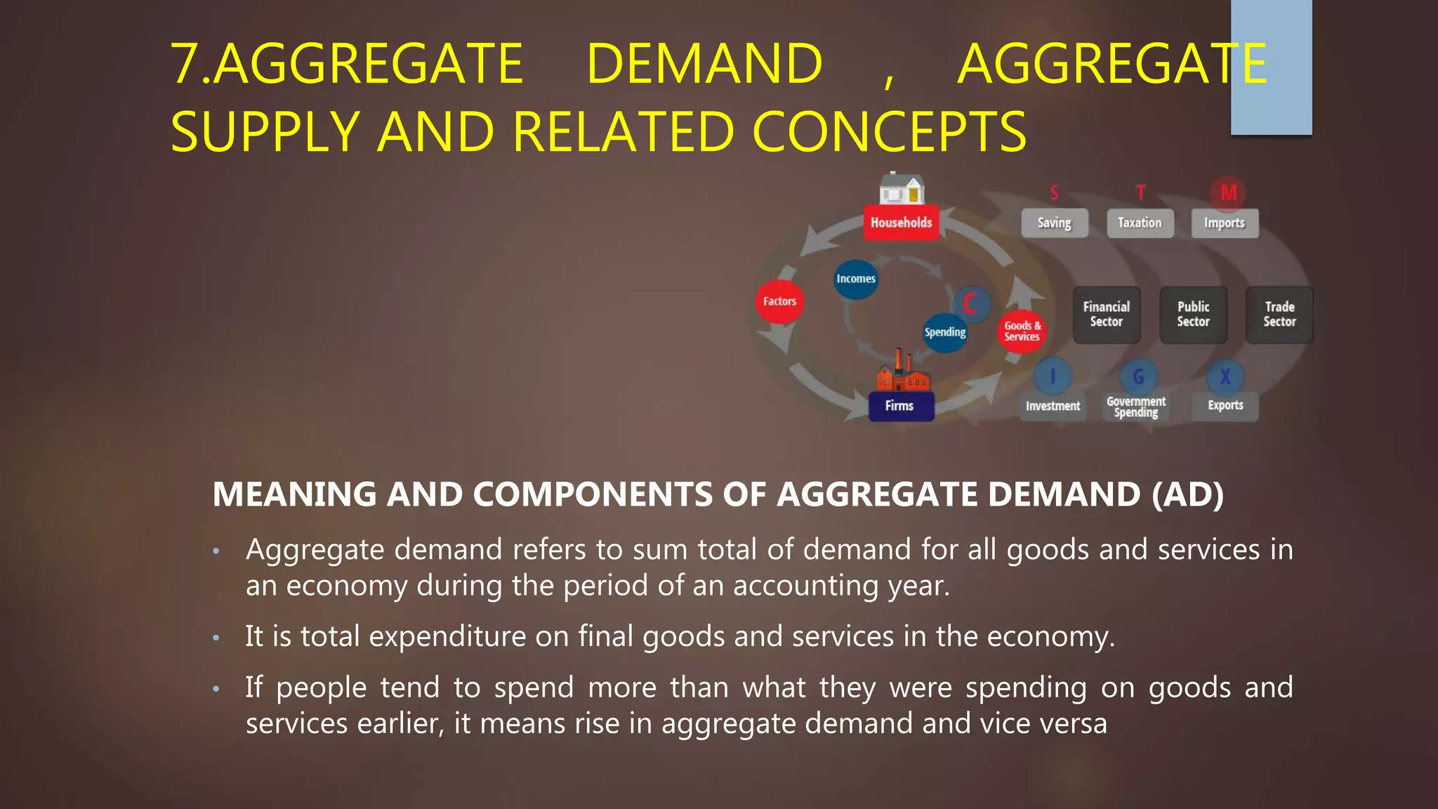
7.AGGREGATE DEMAND , AGGREGATE
SUPPLY AND RELATED CONCEPTS
MEANING AND COMPONENTS OF AGGREGATE DEMAND (AD)
• Aggregate demand refers to sum total of demand for all goods and services in
an economy during the period of an accounting year.
• It is total expenditure on final goods and services in the economy.
• If people tend to spend more than what they were spending on goods and
services earlier, it means rise in aggregate demand and vice versa
A. Relation of Aggregate Demand (AD) with Price Level
 There is a negative relation between them i.e., aggregate demand falls with
increase in the general price level and vice-versa.
B. Relation of Aggregate Demand with Income Level
 There is a positive relation between them i.e., aggregate demand increases
with rise in income level. The curve has positive slope.
Components of Aggregate Demand in a Four Sector
(OPEN)Economy
Aggregate demand refers to aggregate (total) expenditure on goods and
services made in the economy during the accounting period. The four main
components of aggregate demand are:
1. Private Consumption Expenditure
2. Investment Expenditure
3. Government Expenditure
4. Net Exports
1.Private Consumption Expenditure
 It refers to the total expenditure incurred by the households
on the purchase of goods and services during, a given period
of time.
 There is positive relationship between income and
consumption.
 As income rises, consumption also rises and vice versa.
2. Investment Expenditure (I).
 It is total expenditure by the producing sector for the
investment such as purchase of capital goods, plant, machinery
etc.
 It is affected by rate of interest and marginal efficiency of capital
(MEI).
 There is negative relationship between rate of interest and
investment demand."
3.Government Expenditure
It is the total expenditure incurred by government on
• Intermediate consumption of government sector.
• Compensation of employees (C.O.E.) of government sector.
• Imports by the government sector.
• Government expenditure is affected by the government policy.
4. Net Exports (X-M)
 It is the difference between exports and imports of goods and
services.
 It shows the effect of domestic spending on foreign goods and
services (M) and foreign spending on domestic goods and services
(X) on the level of aggregate demand.
Hence ,AD = C+ I+G+(X-M)
Components of Aggregate Demand in a Two-
Sector(CLOSED)
Economy In a two- sector economy, AD has two components :
 Consumption and,
 Investment
Two sector economy comprises:
 Household sector and
 Producer sector,
Thus aggregate demand/aggregate expenditure in a two sector economy is
sum total of consumption and investment.
 Household sector demands for consumption (C)
 Producer sector demands for investment (I)
AD = C+I

Level of
Income Y
Consumption
C
Investment I
Aggregate
Demand AD
(C+I)
0 50 100 150
100 100 100 200
200 150 100 250
300 200 100 300
400 250 100 350
500 300 100 400
The above table is based on assumption that C = 50, b = 0.5,
C = C + bY, C = 50+0.5Y
MEANING AND COMPONENTS OF AGGREGATE SUPPLY (AS]
 AS refers to aggregate production as planned by the producers during an
accounting year .It is the total flow of goods and services in an economy
during a period of one year. Components of aggregate supply are C+S.
 Aggregate supply refers to aggregate production as planned by the
producers during an accounting year.
 We know ,production of goods and services implies ‘value addition’ and value
addition implies imome generation. Our knowledge of national income
accounting tells us that value added and income generation are identical to
each other .
 Accordingly AS AND Y Are identical to each other.,
Y = C+S
or
AS = C+S
Where: C is consumption expenditure S is saving, (Y - C)
Components of Aggregate Supply
1. Consumption (C). It is always positive even when income is zero. When income
increases, consumption increases and vice-versa.
2. Savings (S)S = Y-C. Savings increase with increase in income and vice-versa
There is positive relationship between savings and income.
 Savings may be negative when the level of income is low, i.e., when C > Y.
 Savings are zero when consumption is equal to income, i.e., when C = Y.
 Savings are positive when consumption is less than income, i.e., when C < Y.
Level of Income (Y) Consumption (C ) Savings (S) =(Y-C) Aggregate Supply
(AS) = C+S
0 50 -50 0
100 100 0 100
200 150 50 200
300 200 100 300
400 250 150 400
500 300 200 500
* S = - C + (l - b)Y. Savings can also be calculated by this
equation;
MEANING OF CONSUMPTION FUNCTION/PROPENSITY TO CONSUME
 Consumption function states the relationship between consumption and
income ; C = /(Y)
 According to Keynes,
 "Men are disposed, as a rule and on an average, to increase their
consumption as their income increases, but not as much as increase in
their income."
 It means that as income rises propensity to consume also rises, but by less
than an increase in income.
Observations
1. OY is a 45° line. 45° line has the property that every point on it, is equidistant
from both axes i.e., at each -point, C = Y.
2. Origin of consumption curve. Consumption curve (CQ starts from point C on
the Y- axis. This implies that there is autonomous consumption (C) or OC even
when the income is zero.
3. Slope. CC has a positive slope, which indicates that as income increases,
consumption also rises. Yet, rise in consumption is less than rise in income as
apart of income is saved. The rising slope of consumption curve is
b(MPC = Change in consumption/Change in Income .
4. Break-even point (C = Y). Consumption curve intersects the 45° line at point E,
which is known as the 'Break-even point'. At this point, consumption
expenditure is exactly equal to income. For instance, as per Table, break-even
point occurs corresponding to income of Rs100.
5. When income is less than consumption. To the left of E, consumption is more
than income and deficiency of income leads to dissavings.
6. When income is more than consumption. To the right of point £,
consumption is less than income. Excess of income leads to savings. This
indicates positive savings.
Types of Propensity to Consume
 Propensity to consume refers to a schedule which shows the levels of
consumption at different levels of income in an economy. It is a ratio
between C and Y. It has two aspects/types:
(A).Average Propensity to Consume (APC)
 It is the ratio between total consumption (C) and total income (Y) at a
given level of income in the economy or it is ratio of consumption
expenditure to the corresponding level of income.
APC = Consumption (C)
Income (Y)
 For example, if consumption is Rs60 crore and income is Rs100 crore,
then
APC = 60
100
Means that 60% of income is spent on consumption

Level of Income Consumption APC
0 50 ∞
100 100 1
200 150 0.75
300 200 0.67
400 250 0.625
500 300 0.6
Observations
1. In Table, at the income level of Rs100, the APC is 1.
2. As income rises to Rs200, APC falls to 0.75 and then to 0.67 and
to 0.625 and so on.
3. APC falls as income rises. This is because as income rises,
people tend to save a part of it also.
4. APC is represented at a point on the consumption curve.
Properties/Features of APC
1. APC = 1. At break even point APC = 1 i.e., when C = Y (Rs100
=Rs100).
2. APC > 1. To the left of break-even point, APC > 1 i.e., when
C>Y.
3. APC < 1. To the right of break-even point, APC < 1 i.e., when C
< Y.
4. APC falls with increase in income. It is because proportion of
income spent on consumption keeps on falling (people tend to
save more also).
5. APC can never be zero. This is because consumption is never
zero. Even at zero level of income, autonomous consumption is
there.
(B).Marginal Propensity to Consume (MPC)
 It is the ratio between change in consumption (AC) to change in income
(AY)
MPC =Change in consumption
Change in Income
For example, if income increases from ?200 to ?300 and consumption
increases from Rs80 to Rs140, then
MPC = 140 – 80 = 60= 0.6
300 – 20 100
It indicates that 60% of increase in income is spent on consumption.
Income
Consumpti
on
Change in
Consumptio
n
Change
in
Income
MPC
0 50 - - -
100 100 50 100 0.5
200 150 50 100 0.5
300 200 50 100 0.5
400 250 50 -100 0.5
500 300 50 100 0.5
Observations
1. MPC measures the slope of consumption curve.
2. Constant value of MPC indicates that consumption curve is a
straight line i.e., that MPC/b remains same.
3. MPC is measured by AC/AY between two points i.e., when changing
from one income level to the other.
For example, when moving from point B to C or MPC at point C, with
respect to point B
MPC = Change in Consumption= PP1 = 50 = 0.5
Change in Income YY1 100
Properties/Features of MPC
1. Value of MPC ranges between 0 and 1.
2. If entire additional income is spent, Change in C = Change in Y implying MPC
= 1
3. If entire additional income is saved then Change C=0, implying MPC=0.
4. MPC of developing countries is more than MPC of developed countries as
developing countries need to spend on basic needs more than the developed
countries.
5. It is also said that MPC of poor is more than MPC of rich, as poor person
needs to spend more on basic necessities.
MEANING OF SAVING FUNCTION OR PROPENSITY TO SAVE
• Saving function refers to the relation between saving and income (S
and Y). S = f(Y)
• Saving is the excess of income over and above consumption during
an accounting year. S = Y-C
• Propensity to save refers to the schedule which shows different
levels of savings at different levels of income in an economy.
Income Consumption Savings
0 50 -50
100 100 0
200 150 50
300 200 100
400 250 150
500 300 200
Observations
• Origin of saving curve. Saving starts
from point S on Y axis. It indicates that
there are negative savings when income is
zero.
• Slope. Saving curve has a positive slope
which means that saving and income
move in same direction. With increase in
income, savings increase and vice-versa.
• When savings are zero. Savings are zero
at a point when consumption is equal to
income. This is called break-even point.
Refer to point E1 in Fig.
• When savings are negative. Savings are
negative to the left of break-even point,
when, C>Y.
• When savings are positive. Savings are
positive to the right of break-even
point, when Y > C.
Types of Saving Function/Propensity to Save
There are two aspects or types of saving function or propensity to save
:
 Average Propensity to Save (APS)
 Marginal Propensity to Save (MPS)
(A). Average Propensity to Save (APS)
It is defined as the ratio of total savings to the total income of
the economy.
APS = Savings
Income
For example, if savings are Rs60 crore and income is Rs100
crore,
APS = 60= 0.6
100
Observations
1. APS at the income of Rs100 is zero.
2. As income increases, APS also increases as people tend to
save a larger part as income increases.
3. APS is measured at a point of time.
For example, APS at point C = S= 50 = 0.25
Y 200
Income Consumption Savings APS
0 50 -50 oo
100 100 0 0
200 150 50 0.25
300 200 100 0.33
400 250 150 0.375
500 300 200 0.4
Properties/Feature of APS
1. APS can be zero. APS is zero when savings are zero (C = Y).
2. APS can never be 1. It is because savings can never be equal to income
(as people spend a part of income on consumption).
3. APS can never be more than one. It is because savings can not be more
than income, but APS can be negative (when C > Y).
4. APS rises with rise in income. It is because people tend to save more with
increase in income.
(B).Marginal Propensity to Save (MPS)
 It is defined as the ratio of change in savings resulting from, change in income
of the economy.
MPS = Change in Savings
Change in Income
 For example, if savings increase from Rs40 crore to Rs80 crore and
income increases from Rs100 crore to Rs200 crore, then
MPS = 80 – 40= 40= 0.4
200 –100 100
Observations
1. MPS at the income of ?100 is 0.5.
2. It remains constant at all levels of income.
3. It is measured from one point to the other.
For example, MPS (i.e., at point D with respect to point C) is
= 50 = 0.5
100
Income Savings
Change
in
Savings
(AS)
Change
in
Income
MPS
0 -50 - - -
100 0 50 100 0.5
200 50 50 100 0.5
300 100 50 100 0.5
400 150 50 100 0.5
500 200 50 100 0.5
Properties/Features of MPS
1. MPS varies between 0 and 1.
2. MPS will be equal to 0 if entire additional income is consumed i.e.,
Change in S=0.
3. MPS will be equal to 1 if entire income is saved Change in S = Change
in Y.
4. MPS can not be greater than 1 because Change in S cannot be greater
than Change Y.
DERIVATION OF SAVING FUNCTION/CURVE FROM CONSUMPTION
FUNCTION / CURVE AND CONSUMPTION FUNCTION/CURVE FROM SAVING
FUNCTION/CURVE
We make use of two functions to derive saving curve from consumption curve and
vice versa.
(A). Linear Consumption Function
 When income increases, consumption also increases, but rate of increase in
consumption is less than rate of increase in income.
Algebraically: Consumption function is C = C + bY
(B) Linear Saving Function
 Just like consumption function, saving function is also linear. Saving function
can be derived from consumption function.
Algebraically: Saving function is S = -C + (1 - b)Y
Derivation of Saving Curve from Consumption Curve
Given that CC is the consumption curve and OY is the income curve, we derive
saving curve as following .
1. We take OS = OC as OC is autonomous consumption (C) defined at zero level of
income. It implies that saving at zero level of income will be OS (-C). Thus we get a
point S on negative V axis from where the saving curve will start.
2. Point E on consumption curve indicates break even point (consumption = income)
implying APC = 1 and zero savings. Hence saving curve will intersect X axis at
point E1 (Alternatively perpendicular from point £ to E, may also be drawn).
3. We join points S and E1and by extending the straight line upwards, we get the
saving curve SE1 S or SS.
Derivation of Consumption Curve from Saving Curve
Given that SS is the saving curve. We derive consumption curve as follows.
1. We draw 45° line from the origin OY, the income curve.
2. We take OC = OS, OS being the amount of dissavings (-C). It implies
autonomous consumption (C). Thus we get point C on Y axis from where
the consumptioncurve will start.
3. Point E1 indicates zero savings. Hence consumption curve will intersect
the income curve at point E implying consumption equal to income.
(Alternatively perpendicular from point E1 to point E may also be drawn).
4. We join points C and £ and extend upwards to get consumption curve
CEC or CC.

INVESTMENT FUNCTION
 Investments are additions made to the existing stock of capital. Or It is
the expenditure which increases the real capital stock. Or It is the
expenditure on creation of new capital assets.
Types of Investment
1. Investment can be of two types :
2. Autonomous investment
3. Induced Investment
1. Autonomous Investment
Expenditure on capital goods which is independent of the level of income and
not influenced by expected profitability.
In other words, it is not affected by changes in the level of income and not
induced by profit motive.
• Autonomous investments are generally made by government. The level
of autonomous investments depends upon the fiscal policy of the
government.
• The curve is parallel to X-axis i.e., the amount of investment remains
constant at OA irrespective of change in level of income from OM to
OM, to OM2.
• It is not induced by profit motive.
• It is not affected by changes in level of income.
2. Induced Investment
It is motivated by expected profitability and the level of income in the economy.
It is positively related to the level of income. If there is increase in income then
induced investment will also increase and vice-versa.
• There is positive relationship between induced investment and income i.e.,
when income increases, induced investment increases and vice versa e.g.,
income increases from OM to OM, and investment increases from OA to
OA.
• It is induced by profit motive.
• It is directly affected by change in the level of income.

Basis Autonomous Investment Induced Investment
1 Investors
It is generally done by the government
sector only.
It is generally done by the
private sector and government
sector also.
2 Motive
Autonomous investments are not
influenced by profit.
Induced investment is influenced
by profit motive.
3 Income Elasticity
It is income inelastic i.e, it is
unaffected by changes in the level of
income
It is income elastic i.e., increase
in the level of income raises the
level of induced investment.
4 Curve
Its curve is parallel to X-axis as it is
income inelastic.
It has a positive slope as it is
income elastic.
MEANING OF EX-ANTE SAVING AND EX-ANTE INVESTMENT
Ex-Ante Savings:
 What savers or households plan to save at different levels of income in an
economy. These are intended or planned savings. The amount of planned
savings is shown by saving function.
Ex-Ante Investments:
 What investors or firms plan to invest at different levels of income in the
economy. These are intended or planned investments. The amount of planned
investment is shown by investment demand function.
MEANING OF EX-POST SAVING AND EX-POST INVESTMENT
Ex-postSaving:
• Ex-post saving refers to the actual or realised saving in an economy during a
year.
Ex-post investment:
Ex-post investment refers to the actual or realised investment in an economy during
a year.
• Ex-post saving and Ex-post investment are equal at all levels of income
because it is an accounting identity which means that practically all
savings will be invested.
CONCEPTS OF FULL EMPLOYMENT,VOLUNTARY UNEMPLOYMENTAND
INVOLUNTARY UNEMPLOYMENT
These concepts are important to understand equilibrium level of income at different
levels of employment.
A. Full Employment
It refers to a situation in which all those, who are able and willing to work at the
existing wage rate, are working.
• Full employment is measured in the context of working population only.
• Full employment implies, there is equilibrium in the labour market i.e.,
Demand of labour = Supply of labour.
• Full employment does not imply 100% employment as even under full
employment, there can be two types of unemployment:
Frictional and Structural
1. Frictional Unemployment.
 It occurs during the time period when workers leave one job and join some other
job.
 It arises due to lack of perfect mobility of factors or due to time requirement
needed in search of a job or due to fulfilment of formalities involved in winding
up old job and in joining the new one.
2. Structural Unemployment.
 This is associated with the structural changes in the economy. Human resources
need some training and skill in order to work with new technologies.
 It occurs in the time period when they are not working due to lack of knowledge
required to work. There is no shortage of work, but there is mismatch between
the supply and demand of the human resources (labour).
B. Voluntary Unemployment
• It refers to a situation when a person is not willing to work at the existing
wage rate.
• When workers are unwilling to accept any work though they are physically
and mentally capable.
• Voluntaryunemployment is not counted
• while measuring the size of unemployment.
C. Involuntary Unemployment
• It refers to a situation in which all those, who are willing and able to work at
the existing wage rate, do not get work.
• Though physically and mentally fit, they are rendered unemployed against
their willingness to work.
• Involuntary unemployment is taken into account while estimating the total
unemployment in an economy.
MACROECOMICS

MACROECOMICS

  • 1.
    7.AGGREGATE DEMAND ,AGGREGATE SUPPLY AND RELATED CONCEPTS MEANING AND COMPONENTS OF AGGREGATE DEMAND (AD) • Aggregate demand refers to sum total of demand for all goods and services in an economy during the period of an accounting year. • It is total expenditure on final goods and services in the economy. • If people tend to spend more than what they were spending on goods and services earlier, it means rise in aggregate demand and vice versa
  • 2.
    A. Relation ofAggregate Demand (AD) with Price Level  There is a negative relation between them i.e., aggregate demand falls with increase in the general price level and vice-versa. B. Relation of Aggregate Demand with Income Level  There is a positive relation between them i.e., aggregate demand increases with rise in income level. The curve has positive slope.
  • 3.
    Components of AggregateDemand in a Four Sector (OPEN)Economy Aggregate demand refers to aggregate (total) expenditure on goods and services made in the economy during the accounting period. The four main components of aggregate demand are: 1. Private Consumption Expenditure 2. Investment Expenditure 3. Government Expenditure 4. Net Exports
  • 4.
    1.Private Consumption Expenditure It refers to the total expenditure incurred by the households on the purchase of goods and services during, a given period of time.  There is positive relationship between income and consumption.  As income rises, consumption also rises and vice versa.
  • 5.
    2. Investment Expenditure(I).  It is total expenditure by the producing sector for the investment such as purchase of capital goods, plant, machinery etc.  It is affected by rate of interest and marginal efficiency of capital (MEI).  There is negative relationship between rate of interest and investment demand."
  • 6.
    3.Government Expenditure It isthe total expenditure incurred by government on • Intermediate consumption of government sector. • Compensation of employees (C.O.E.) of government sector. • Imports by the government sector. • Government expenditure is affected by the government policy.
  • 7.
    4. Net Exports(X-M)  It is the difference between exports and imports of goods and services.  It shows the effect of domestic spending on foreign goods and services (M) and foreign spending on domestic goods and services (X) on the level of aggregate demand. Hence ,AD = C+ I+G+(X-M)
  • 8.
    Components of AggregateDemand in a Two- Sector(CLOSED) Economy In a two- sector economy, AD has two components :  Consumption and,  Investment Two sector economy comprises:  Household sector and  Producer sector, Thus aggregate demand/aggregate expenditure in a two sector economy is sum total of consumption and investment.  Household sector demands for consumption (C)  Producer sector demands for investment (I) AD = C+I
  • 9.
     Level of Income Y Consumption C InvestmentI Aggregate Demand AD (C+I) 0 50 100 150 100 100 100 200 200 150 100 250 300 200 100 300 400 250 100 350 500 300 100 400 The above table is based on assumption that C = 50, b = 0.5, C = C + bY, C = 50+0.5Y
  • 13.
    MEANING AND COMPONENTSOF AGGREGATE SUPPLY (AS]  AS refers to aggregate production as planned by the producers during an accounting year .It is the total flow of goods and services in an economy during a period of one year. Components of aggregate supply are C+S.  Aggregate supply refers to aggregate production as planned by the producers during an accounting year.  We know ,production of goods and services implies ‘value addition’ and value addition implies imome generation. Our knowledge of national income accounting tells us that value added and income generation are identical to each other .  Accordingly AS AND Y Are identical to each other., Y = C+S or AS = C+S Where: C is consumption expenditure S is saving, (Y - C)
  • 14.
    Components of AggregateSupply 1. Consumption (C). It is always positive even when income is zero. When income increases, consumption increases and vice-versa. 2. Savings (S)S = Y-C. Savings increase with increase in income and vice-versa There is positive relationship between savings and income.  Savings may be negative when the level of income is low, i.e., when C > Y.  Savings are zero when consumption is equal to income, i.e., when C = Y.  Savings are positive when consumption is less than income, i.e., when C < Y. Level of Income (Y) Consumption (C ) Savings (S) =(Y-C) Aggregate Supply (AS) = C+S 0 50 -50 0 100 100 0 100 200 150 50 200 300 200 100 300 400 250 150 400 500 300 200 500
  • 15.
    * S =- C + (l - b)Y. Savings can also be calculated by this equation;
  • 16.
    MEANING OF CONSUMPTIONFUNCTION/PROPENSITY TO CONSUME  Consumption function states the relationship between consumption and income ; C = /(Y)  According to Keynes,  "Men are disposed, as a rule and on an average, to increase their consumption as their income increases, but not as much as increase in their income."  It means that as income rises propensity to consume also rises, but by less than an increase in income.
  • 17.
    Observations 1. OY isa 45° line. 45° line has the property that every point on it, is equidistant from both axes i.e., at each -point, C = Y. 2. Origin of consumption curve. Consumption curve (CQ starts from point C on the Y- axis. This implies that there is autonomous consumption (C) or OC even when the income is zero. 3. Slope. CC has a positive slope, which indicates that as income increases, consumption also rises. Yet, rise in consumption is less than rise in income as apart of income is saved. The rising slope of consumption curve is b(MPC = Change in consumption/Change in Income . 4. Break-even point (C = Y). Consumption curve intersects the 45° line at point E, which is known as the 'Break-even point'. At this point, consumption expenditure is exactly equal to income. For instance, as per Table, break-even point occurs corresponding to income of Rs100. 5. When income is less than consumption. To the left of E, consumption is more than income and deficiency of income leads to dissavings. 6. When income is more than consumption. To the right of point £, consumption is less than income. Excess of income leads to savings. This indicates positive savings.
  • 18.
    Types of Propensityto Consume  Propensity to consume refers to a schedule which shows the levels of consumption at different levels of income in an economy. It is a ratio between C and Y. It has two aspects/types: (A).Average Propensity to Consume (APC)  It is the ratio between total consumption (C) and total income (Y) at a given level of income in the economy or it is ratio of consumption expenditure to the corresponding level of income. APC = Consumption (C) Income (Y)  For example, if consumption is Rs60 crore and income is Rs100 crore, then APC = 60 100 Means that 60% of income is spent on consumption
  • 19.
     Level of IncomeConsumption APC 0 50 ∞ 100 100 1 200 150 0.75 300 200 0.67 400 250 0.625 500 300 0.6 Observations 1. In Table, at the income level of Rs100, the APC is 1. 2. As income rises to Rs200, APC falls to 0.75 and then to 0.67 and to 0.625 and so on. 3. APC falls as income rises. This is because as income rises, people tend to save a part of it also. 4. APC is represented at a point on the consumption curve.
  • 20.
    Properties/Features of APC 1.APC = 1. At break even point APC = 1 i.e., when C = Y (Rs100 =Rs100). 2. APC > 1. To the left of break-even point, APC > 1 i.e., when C>Y. 3. APC < 1. To the right of break-even point, APC < 1 i.e., when C < Y. 4. APC falls with increase in income. It is because proportion of income spent on consumption keeps on falling (people tend to save more also). 5. APC can never be zero. This is because consumption is never zero. Even at zero level of income, autonomous consumption is there.
  • 21.
    (B).Marginal Propensity toConsume (MPC)  It is the ratio between change in consumption (AC) to change in income (AY) MPC =Change in consumption Change in Income For example, if income increases from ?200 to ?300 and consumption increases from Rs80 to Rs140, then MPC = 140 – 80 = 60= 0.6 300 – 20 100 It indicates that 60% of increase in income is spent on consumption.
  • 22.
    Income Consumpti on Change in Consumptio n Change in Income MPC 0 50- - - 100 100 50 100 0.5 200 150 50 100 0.5 300 200 50 100 0.5 400 250 50 -100 0.5 500 300 50 100 0.5 Observations 1. MPC measures the slope of consumption curve. 2. Constant value of MPC indicates that consumption curve is a straight line i.e., that MPC/b remains same. 3. MPC is measured by AC/AY between two points i.e., when changing from one income level to the other. For example, when moving from point B to C or MPC at point C, with respect to point B MPC = Change in Consumption= PP1 = 50 = 0.5 Change in Income YY1 100
  • 23.
    Properties/Features of MPC 1.Value of MPC ranges between 0 and 1. 2. If entire additional income is spent, Change in C = Change in Y implying MPC = 1 3. If entire additional income is saved then Change C=0, implying MPC=0. 4. MPC of developing countries is more than MPC of developed countries as developing countries need to spend on basic needs more than the developed countries. 5. It is also said that MPC of poor is more than MPC of rich, as poor person needs to spend more on basic necessities.
  • 24.
    MEANING OF SAVINGFUNCTION OR PROPENSITY TO SAVE • Saving function refers to the relation between saving and income (S and Y). S = f(Y) • Saving is the excess of income over and above consumption during an accounting year. S = Y-C • Propensity to save refers to the schedule which shows different levels of savings at different levels of income in an economy. Income Consumption Savings 0 50 -50 100 100 0 200 150 50 300 200 100 400 250 150 500 300 200
  • 25.
    Observations • Origin ofsaving curve. Saving starts from point S on Y axis. It indicates that there are negative savings when income is zero. • Slope. Saving curve has a positive slope which means that saving and income move in same direction. With increase in income, savings increase and vice-versa. • When savings are zero. Savings are zero at a point when consumption is equal to income. This is called break-even point. Refer to point E1 in Fig. • When savings are negative. Savings are negative to the left of break-even point, when, C>Y. • When savings are positive. Savings are positive to the right of break-even point, when Y > C.
  • 26.
    Types of SavingFunction/Propensity to Save There are two aspects or types of saving function or propensity to save :  Average Propensity to Save (APS)  Marginal Propensity to Save (MPS) (A). Average Propensity to Save (APS) It is defined as the ratio of total savings to the total income of the economy. APS = Savings Income For example, if savings are Rs60 crore and income is Rs100 crore, APS = 60= 0.6 100
  • 27.
    Observations 1. APS atthe income of Rs100 is zero. 2. As income increases, APS also increases as people tend to save a larger part as income increases. 3. APS is measured at a point of time. For example, APS at point C = S= 50 = 0.25 Y 200 Income Consumption Savings APS 0 50 -50 oo 100 100 0 0 200 150 50 0.25 300 200 100 0.33 400 250 150 0.375 500 300 200 0.4
  • 28.
    Properties/Feature of APS 1.APS can be zero. APS is zero when savings are zero (C = Y). 2. APS can never be 1. It is because savings can never be equal to income (as people spend a part of income on consumption). 3. APS can never be more than one. It is because savings can not be more than income, but APS can be negative (when C > Y). 4. APS rises with rise in income. It is because people tend to save more with increase in income.
  • 29.
    (B).Marginal Propensity toSave (MPS)  It is defined as the ratio of change in savings resulting from, change in income of the economy. MPS = Change in Savings Change in Income  For example, if savings increase from Rs40 crore to Rs80 crore and income increases from Rs100 crore to Rs200 crore, then MPS = 80 – 40= 40= 0.4 200 –100 100
  • 30.
    Observations 1. MPS atthe income of ?100 is 0.5. 2. It remains constant at all levels of income. 3. It is measured from one point to the other. For example, MPS (i.e., at point D with respect to point C) is = 50 = 0.5 100 Income Savings Change in Savings (AS) Change in Income MPS 0 -50 - - - 100 0 50 100 0.5 200 50 50 100 0.5 300 100 50 100 0.5 400 150 50 100 0.5 500 200 50 100 0.5
  • 31.
    Properties/Features of MPS 1.MPS varies between 0 and 1. 2. MPS will be equal to 0 if entire additional income is consumed i.e., Change in S=0. 3. MPS will be equal to 1 if entire income is saved Change in S = Change in Y. 4. MPS can not be greater than 1 because Change in S cannot be greater than Change Y.
  • 32.
    DERIVATION OF SAVINGFUNCTION/CURVE FROM CONSUMPTION FUNCTION / CURVE AND CONSUMPTION FUNCTION/CURVE FROM SAVING FUNCTION/CURVE We make use of two functions to derive saving curve from consumption curve and vice versa. (A). Linear Consumption Function  When income increases, consumption also increases, but rate of increase in consumption is less than rate of increase in income. Algebraically: Consumption function is C = C + bY (B) Linear Saving Function  Just like consumption function, saving function is also linear. Saving function can be derived from consumption function. Algebraically: Saving function is S = -C + (1 - b)Y
  • 33.
    Derivation of SavingCurve from Consumption Curve Given that CC is the consumption curve and OY is the income curve, we derive saving curve as following . 1. We take OS = OC as OC is autonomous consumption (C) defined at zero level of income. It implies that saving at zero level of income will be OS (-C). Thus we get a point S on negative V axis from where the saving curve will start. 2. Point E on consumption curve indicates break even point (consumption = income) implying APC = 1 and zero savings. Hence saving curve will intersect X axis at point E1 (Alternatively perpendicular from point £ to E, may also be drawn). 3. We join points S and E1and by extending the straight line upwards, we get the saving curve SE1 S or SS.
  • 34.
    Derivation of ConsumptionCurve from Saving Curve Given that SS is the saving curve. We derive consumption curve as follows. 1. We draw 45° line from the origin OY, the income curve. 2. We take OC = OS, OS being the amount of dissavings (-C). It implies autonomous consumption (C). Thus we get point C on Y axis from where the consumptioncurve will start. 3. Point E1 indicates zero savings. Hence consumption curve will intersect the income curve at point E implying consumption equal to income. (Alternatively perpendicular from point E1 to point E may also be drawn). 4. We join points C and £ and extend upwards to get consumption curve CEC or CC.
  • 36.
  • 37.
    INVESTMENT FUNCTION  Investmentsare additions made to the existing stock of capital. Or It is the expenditure which increases the real capital stock. Or It is the expenditure on creation of new capital assets. Types of Investment 1. Investment can be of two types : 2. Autonomous investment 3. Induced Investment
  • 38.
    1. Autonomous Investment Expenditureon capital goods which is independent of the level of income and not influenced by expected profitability. In other words, it is not affected by changes in the level of income and not induced by profit motive. • Autonomous investments are generally made by government. The level of autonomous investments depends upon the fiscal policy of the government. • The curve is parallel to X-axis i.e., the amount of investment remains constant at OA irrespective of change in level of income from OM to OM, to OM2. • It is not induced by profit motive. • It is not affected by changes in level of income.
  • 39.
    2. Induced Investment Itis motivated by expected profitability and the level of income in the economy. It is positively related to the level of income. If there is increase in income then induced investment will also increase and vice-versa. • There is positive relationship between induced investment and income i.e., when income increases, induced investment increases and vice versa e.g., income increases from OM to OM, and investment increases from OA to OA. • It is induced by profit motive. • It is directly affected by change in the level of income.
  • 40.
     Basis Autonomous InvestmentInduced Investment 1 Investors It is generally done by the government sector only. It is generally done by the private sector and government sector also. 2 Motive Autonomous investments are not influenced by profit. Induced investment is influenced by profit motive. 3 Income Elasticity It is income inelastic i.e, it is unaffected by changes in the level of income It is income elastic i.e., increase in the level of income raises the level of induced investment. 4 Curve Its curve is parallel to X-axis as it is income inelastic. It has a positive slope as it is income elastic.
  • 41.
    MEANING OF EX-ANTESAVING AND EX-ANTE INVESTMENT Ex-Ante Savings:  What savers or households plan to save at different levels of income in an economy. These are intended or planned savings. The amount of planned savings is shown by saving function. Ex-Ante Investments:  What investors or firms plan to invest at different levels of income in the economy. These are intended or planned investments. The amount of planned investment is shown by investment demand function.
  • 42.
    MEANING OF EX-POSTSAVING AND EX-POST INVESTMENT Ex-postSaving: • Ex-post saving refers to the actual or realised saving in an economy during a year. Ex-post investment: Ex-post investment refers to the actual or realised investment in an economy during a year. • Ex-post saving and Ex-post investment are equal at all levels of income because it is an accounting identity which means that practically all savings will be invested.
  • 43.
    CONCEPTS OF FULLEMPLOYMENT,VOLUNTARY UNEMPLOYMENTAND INVOLUNTARY UNEMPLOYMENT These concepts are important to understand equilibrium level of income at different levels of employment. A. Full Employment It refers to a situation in which all those, who are able and willing to work at the existing wage rate, are working. • Full employment is measured in the context of working population only. • Full employment implies, there is equilibrium in the labour market i.e., Demand of labour = Supply of labour. • Full employment does not imply 100% employment as even under full employment, there can be two types of unemployment: Frictional and Structural
  • 44.
    1. Frictional Unemployment. It occurs during the time period when workers leave one job and join some other job.  It arises due to lack of perfect mobility of factors or due to time requirement needed in search of a job or due to fulfilment of formalities involved in winding up old job and in joining the new one. 2. Structural Unemployment.  This is associated with the structural changes in the economy. Human resources need some training and skill in order to work with new technologies.  It occurs in the time period when they are not working due to lack of knowledge required to work. There is no shortage of work, but there is mismatch between the supply and demand of the human resources (labour).
  • 45.
    B. Voluntary Unemployment •It refers to a situation when a person is not willing to work at the existing wage rate. • When workers are unwilling to accept any work though they are physically and mentally capable. • Voluntaryunemployment is not counted • while measuring the size of unemployment. C. Involuntary Unemployment • It refers to a situation in which all those, who are willing and able to work at the existing wage rate, do not get work. • Though physically and mentally fit, they are rendered unemployed against their willingness to work. • Involuntary unemployment is taken into account while estimating the total unemployment in an economy.

Editor's Notes