Download to read offline

![• Pearson correlation coefficient
– r
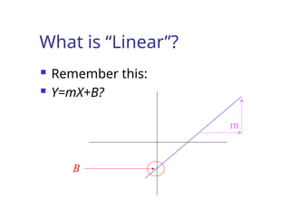
– Linear relationship
)
)(
(
)]
)(
[(
Y
X
Y
X
SS
SS
M
Y
M
X
r
](https://image.slidesharecdn.com/lecture-10-correlation-and-regression-240907190141-635a25ba/85/lecture-10-Correlation-and-Regression-ppt-27-320.jpg)
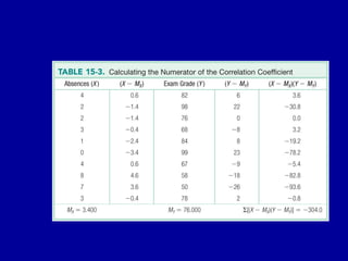
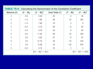
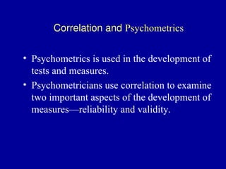
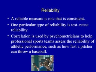
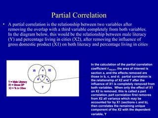
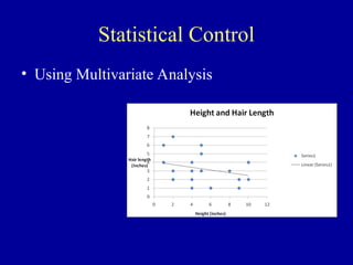
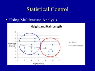

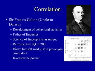
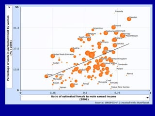
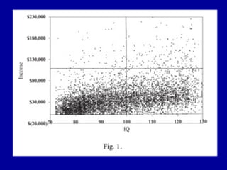
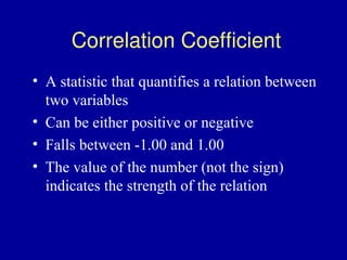
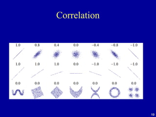
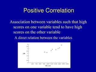
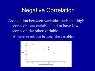
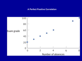
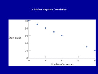
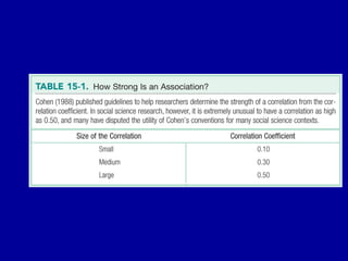
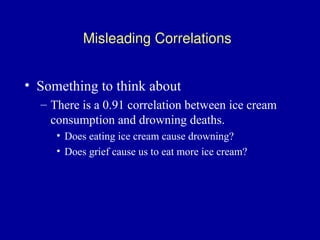
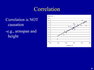
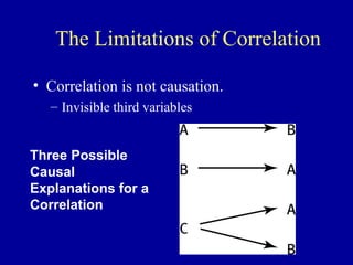
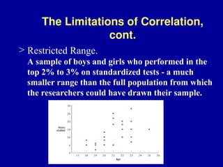
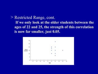
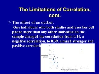
The document discusses the concept of correlation, its statistical measurement, and its applications in psychology and education. It differentiates between positive and negative correlations, highlights the limitations of correlation, and emphasizes that correlation does not imply causation. Techniques such as partial correlation and statistical control are also addressed, along with examples of misleading correlations and the importance of considering additional variables.