Lec10 matching

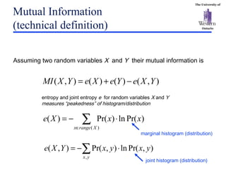
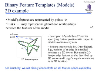
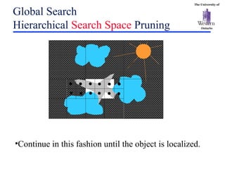
The University of
Ontario
CS 433/557
Algorithms for Image Analysis
Template Matching
Acknowledgements: Dan Huttenlocher

The University of
Ontario
CS 433/557 Algorithms for Image Analysis
Matching and Registration
Template Matching
• intensity based (correlation measures)
• feature based (distance transforms)
Flexible Templates
• pictorial structures
– Dynamic Programming on trees
– generalized distance transforms
Extra Material:

The University of
Ontario
Intensity Based Template Matching
Basic Idea
Left ventricle template
Find best template “position” in the image
Face template
image
image

The University of
Ontario
Intensity-Based
Rigid Template matching
image
coordinate
system s
template
coordinate
system
pixel p in
template T
pixel p+s
in image
For each position s of the template compute
some goodness of “match” measure Q(s)
2
|)()(|1
1
)(
pTspI
sQ
Tp
∑∈
−+⋅+
=
α
e.g. sum of
squared
differences
Sum over all pixels p in template T

The University of
Ontario
Intensity-Based
image
coordinate
system
s1
template
coordinate
system
s2
)2()1( sQsQ <
Search over all plausible positions s and find the optimal
one that has the largest goodness of match value Q(s)

The University of
Ontario
Intensity-Based
What if intensities of your image are not exactly the
same as in the template? (e.g. may happen due to
different gain setting at image acquisition)

The University of
Ontario
Other intensity based
goodness of match measures
Normalized correlation
Mutual Information (next slide)
)()()()(
)()(
)(
pTpTspIspI
pTspI
sQ
Tp
⋅⋅+⋅+
⋅+
=
∑∈

The University of
Ontario
Other goodness of match measures :
Mutual Information
Will work even in extreme cases
In this example the spatial structure of template
and image object are similar while actual
intensities are completely different

The University of
Ontario
Other goodness of match measures :
Mutual Information
Fix s and consider joint histogram of intensity “pairs”: TpforIT spp ∈+ ),(
s1
•Mutual information between template T and image I (for given transformation s)
describes “peakedness” of the joint histogram
•measures how well spatial structures in T and I align
s2
Joint histogram is more
concentrated (peaked)
for s2
T
I
T
I
Joint histogram is spread-out
for s1
T
I

The University of
Ontario
Mutual Information
(technical definition)
),()()(),( YXeYeXeYXMI −+=
∑∈
⋅−=
)(
)Pr(ln)Pr()(
Xrangex
xxXe
∑ ⋅−=
yx
yxyxYXe
,
),Pr(ln),Pr(),(
entropy and joint entropy e for random variables X and Y
measures “peakedness” of histogram/distribution
Assuming two random variables X and Y their mutual information is
joint histogram (distribution)
marginal histogram (distribution)

The University of
Ontario
Mutual Information
Computing MI for a given position s
∑ ⋅
yx yx
yx
yx
, )Pr()Pr(
),Pr(
ln),Pr(
•We want to find s that maximizes MI that can be written as
T
I
joint distribution Pr(x,y)
(normalized histogram)
for a fixed given s
NOTE: has to be careful when computing.
For example, what if H(x,y)=0 for a given pair (x,y)?
∑=
y
yxx ),Pr()Pr( ∑=
x
yxy ),Pr()Pr(
marginal distributions Pr(x) and Pr(y)

The University of
OntarioFinding optimal template position s
Need to search over all feasible values of s
• Template T could be large
– The bigger the template T the more time we spend
computing goodness of match measure at each s
• Search space (of feasible positions s) could be huge
– Besides translation/shift, position s could include scale,
rotation angle, and other parameters (e.g. shear)
Q: Efficient search over all s?

The University of
OntarioFinding optimal template position s
One possible solution: Hierarchical Approach
1. Subsample both template and image.
Note that the search space can be
significantly reduced. The template
size is also reduced.
2. Once a good solution(s) is found at a
corser scale, go to a finer scale. Refine
the search in the neighborhood of the
courser scale solution.

The University of
OntarioFeature Based Template Matching
Features: edges, corners,… (found via filtering)
Distance transforms of binary images
Chamfer and Housdorff matching
Iterated Closed Points

The University of
Ontario
Feature-based Binary Templates/Models
What are they?
What are features?
• Object edges, corners, junctions, e.t.c.
– Features can be detected by the corresponding image filters
• Intensity can also be a considered a feature but it may not
be very robust (e.g. due to illumination changes)
A model (binary template) is a set of feature
points in N-dimensional
space (also called feature space)
• Each feature is defined by a descriptor (vector)
{ } N
n RMMM ⊂= ,...,1
N
i RM ∈

The University of
Ontario
Binary Feature Templates (Models)
2D example
• Links may represent neighborhood relationships
between the features of the model
• Model’s features are represented by points
– descriptor could be a 2D vector
specifying feature position with respect to
model’s coordinate system
– Feature spaces could be 3D (or higher).
E.g., position of an edge in a medical
volumes is a 3D vector. But even in 2D
images edge features can be described by
3D vectors (add edge’s angular orientation
to its 2D location)
reference
point
iM
jM
iM
2D feature space
For simplicity, we will mainly concentrate on 2D feature space examples
iM

The University of
OntarioMatching Binary Template to Image
iM
L
L - model’s positioning
iML⊕ - position of feature i
At fixed position L we can
compute match quality Q(L)
using some goodness of
match criteria.
Example: Q(L) = number of (exact)
matches (in red) between model and
image features (e.g. edges).
Object is detected at all
positions which are local
maxima of function Q(L)
such that where
K is some presence threshold
Lˆ
KLQ >)ˆ(

The University of
OntarioExact feature matching is not robust
iM
L
Counting exact matches may be sensitive to even minor deviation
in shape between the model and the actual object appearance

The University of
OntarioDistance Transform
More robust goodness of match measures use
distance transform of image features
1. Detect desirable image features
(edges, corners, e.t.c.) using
appropriate filters
2. For all image pixels p find
distance D(p) to the nearest
image feature
p
0)( =pD
q
0)( >qD
)()( qDsD >
s

The University of
3
4
2
3
2
3
5 4 4
2
2
3
1
1
2
2 1 1 2 1
1 0 0 1 2 1
0
0
0
1
232101
1 0 1 2 3 3 2
1
0
1
1
1
0 1
2
1 0 1 2 3 4 3 2
1
0
1
2
2
Distance TransformImage features (2D)
Distance Transform is a function that for each image
pixel p assigns a non-negative number corresponding to
distance from p to the nearest feature in the image I
)(⋅ID
)(pDI

The University of
Image features
(edges)
Distance Transform
Distance Transform can be
visualized as a gray-scale image
ID
ID

The University of
Ontario
Distance Transform
can be very efficiently computed

The University of
Ontario
Metric properties of
discrete Distance Transforms
- 1
1 0
0 1
1 -
Forward
mask
Backward
mask
Manhattan (L1) metric
Set of equidistant
points
Metric
1.4 1
1 0
1.4 0
1.4 1
1
1.4
Better approximation
of Euclidean metric
Exact Euclidean Distance transform
can be computed fairly efficiently (in
linear time) without bigger masks.
www.cs.cornell.edu/~dph/matchalgs/
Euclidean (L2) metric

The University of
Ontario
Goodness of Match via
Distance Transforms
At each model position one can “probe” distance transform
values at locations specified by model (template) features
3
4
2
3
2
3
5 4 4
2
2
3
1
1
2
2 1 1 2 1
1 0 0 1 2 1
0
0
0
1
232101
1 0 1 2 3 3 2
1
0
1
1
1
0 1
2
1 0 1 2 3 4 3 2
1
0
1
2
2
Use distance transform
values as evidence of
proximity to image features.

The University of
Ontario
Goodness of Match Measures
using Distance Transforms
Chamfer Measure
• sum distance transform values “probed” by template features
Hausdorff Measure
• k-th largest value of the distance transform at locations
“probed” by template features
• (Equivalently) number of template features with “probed”
distance transform values less than fixed (small) threshold
– Count template features “sufficiently” close to image features
Spatially coherent matching

The University of
OntarioHausdorff Matching
counting matches with a dialated set of image features

The University of
OntarioSpatial Coherence of Feature Matches
50%
matched
50%
matched
'L "L
Spatially incoherent
matches
Spatially incoherent
matches
• Few “discontinuities” between
neighboring features
• Neighborhood is defined by links
between template/model features
Spatial coherence:

The University of
OntarioSpatially Coherent Matching
Separate template/model features into three subsets
Count the number of non-boundary matchable features
•Matchable (red)
-near image features
•Boundary (blue circle)
-matchable but “near” un-matchable
-links define “near” for model features
•Un-matchable (gray)
-far from image features

The University of
Ontario
L
Spatially Coherent Matching
L
Percentage of non-boundary matchable features
(spatially coherent matches)
%0 %50≈

The University of
OntarioComparing different match measures
Binary model
(edges)
5% clutter image
• Monte Carlo experiments with known
object location and synthetic clutter and
occlusion
-Matching edge locations
• Varying percent clutter
-Probability of edge pixel 2.5-15%
• Varying occlusion
-Single missing interval 10-25% of the
boundary
• Search over location, scale, orientation

The University of
Ontario
Comparing different match measures:
ROC curves
Probability of false alarm versus detection
- 10% and 15% of occlusion with 5% clutter
-Chamfer is lowest, Hausdorff (f=0.8) is highest
-Chamfer truncated distance better than trimmed

The University of
Ontario
ROC’s for
Spatial Coherence Matching
Clutter 3%
Occlusion 20%
FA
CD
0 1
1
Clutter 5%
Occlusion 20%
0=β
0>β
Clutter 5%
Occlusion 40%
0=β
0>β
Clutter 3%
Occlusion 40%
0=β
0>β
FA
CD
0 1
1
FA
CD
0 1
1
FA
CD
0 1
1
• Parameter
defined degree of
connectivity between
model features
• If then
model
features are not
connected at all. In
this case, spatially
coherent matching
reduces to plain
Hausdorff matching.
0=β
β

The University of
OntarioEdge Orientation Information
Match edge orientation (in addition to location)
• Edge normals or gradient direction
3D model feature space (2D location + orientation)
Extract 3D (edge) features from image as well.
Requires 3D distance transform of image features
• weight orientation versus location
• fast forward-backward pass algorithm applies
Increases detection robustness and speeds up matching
• better able to discriminate object from clutter
• better able to eliminate cells in branch and bound search

The University of
OntarioROC’s for Oriented Edge Pixels
Vast Improvement for moderate clutter
• Images with 5% randomly generated contours
• Good for 20-25% occlusion rather than 2-5%
Oriented Edges Location only

The University of
Ontario
Efficient search for
good matching positions L
Distance transform of observed image features needs to
be computed only once (fast operation).
Need to compute match quality for all possible
template/model locations L (global search)
• Use hierarchical approach to efficiently prune the search space.
Alternatively, gradient descent from a given initial
position (e.g. Iterative Closest Point algorithm, …later)
• Easily gets stuck at local minima
• Sensitive to initialization

The University of
Ontario
Global Search
Hierarchical Search Space Pruning
Assume that the entire box might be pruned out if the
match quality is sufficiently bad in the center of the box
(how? … in a moment)

The University of
Ontario
Global Search
If a box is not pruned then subdivide it into smaller
boxes and test the centers of these smaller boxes.

The University of
Ontario
Global Search
•Continue in this fashion until the object is localized.

The University of
Ontario
Pruning a Box
(preliminary technicality)
Location L’ is uniformly better than L” if
for all model features i
A uniformly better location is guaranteed to have better match quality!
5 6 7 7 7
6 6
2
4
3
4
1
2
0
1 0 1
0
5
1
2
3
4
4
4
3
2
1
1
0
1
3
3
4
1
1
2
0
1
L’
)"()'( iIiI MLDMLD ⊕≤⊕
L”
9 10 11 10 9
8 7
12
9
11
10
11
8
10
7 6 5
4
8
3
2
3
4
5
4
3
2
1
1
0
1
6
7
8
3
4
5
2
9

The University of
Ontario
Pruning a Box
(preliminary technicality)
7
5 6 7 6 5
4 3
8
5
6
7
4
6
3 2 1
0
4
0
0
0
0
1
0
0
0
0
0
0
0
2
3
4
0
0
1
0
5
λ
hypothetical
location
Assume that is uniformly better than any location
then the match quality satisfies for any
If the presence test fails ( for a given threshold K)
then any location must also fail the test
The entire box can be pruned by one test at !!!!λ
BoxL∈
λ BoxL∈
Assume that
is uniformly better than any
location in the box
λ
KQ <)(λ
)()( LQQ ≥λ BoxL∈

The University of
OntarioBuilding “ “ for a Box of “Radius” n
at the center
of the box
9 10 11 10 9
8 7
12
9
11
10
11
8
10
7 6 5
4
8
3
2
3
4
5
4
3
2
1
1
0
1
6
7
8
3
4
5
2
9
• value of the distance transform changes at most by 1 between neighboring
pixels
λ
BoxLanyforMLDnpD ii ∈+≤− ),())((
)( ipD• value of can decrease by at most n (box radius) for other box positions
)( ipD 7
5 6 7 6 5
4 3
8
5
6
7
4
6
3 2 1
0
4
0
0
0
0
1
0
0
0
0
0
0
0
2
3
4
0
0
1
0
5
λ
hypothetical
location
{ }0,))((max npD i −

The University of
Ontario
Global Hierarchical Search
(Branch and Bound)
Hierarchical search works in more
general case where “position” L
includes translation, scale, and
orientation of the model
• N-dimensional search space
Guaranteed or admissible search
heuristic
• Bound on how good answer could be in
unexplored region
– can not miss an answer
• In worst case won’t rule anything out
In practice rule out vast majority of
template locations (transformations)

The University of
Ontario
Local Search (gradient descent):
Iterated Closest Point algorithm
ICP: Iterate until convergence
1. Estimate correspondence between each template feature i and
some image feature located at F(i) (Fitzgibbons: use DT)
2. Move model to minimize the sum of distances between the
corresponding features (like chamfer matching)
Alternatively, find local move of the model
improving DT-based match quality function Q(L)
)(~ LQL −∇∆
L∆
i
)(iF
∑ −⊕∇−∆
i
i iFMLL 2
))()((~

The University of
Ontario
Problems with ICP
and gradient descent matching
Slow
• Can take many iterations
• ICP: each iteration is slow due to search for
correspondences
– Fitzgibbons: improve this by using DT
No convergence guarantees
• Can get stuck in local minima
– Not much to do about this
– Can be improved by using robust distance measures (e.g.
truncated Euclidean measure)

The University of
OntarioObservations on DT based matching
Main point of DT: allows to measure match quality
without explicitly finding correspondence between pairs
of mode and image features (hard problem!)
Hierarchical search over entire transformation space
Important to use robust distance
• Straight Chamfer very sensitive to outliers
• Truncated DT can be computed very fast
Fast exact or approximate methods for DT ( metric)
For edge features use orientation too
• edge normals or intensity gradients
2L

The University of
Ontario
Rigid 2D templates
Should we really care?
So far we studied matching in case of 2D images
and rigid 2D templates/models of objects
• When do rigid 2D templates work?
– there are rigid 2D objects (e.g. fingerprints)
– 3D object may be imaged from the same view point:
• controlled image-based data bases (e.g. photos of employees,
criminals)
• 2D satellite images always view 3D objects from above
• X-Rays, microscope photography, e.t.c.

The University of
OntarioMore general 3D objects
3D image volumes and 3D objects
• Distance transforms, DT-based matching criteria,
and hierarchical search techniques easily generalize
• Mainly medical applications
2D image and 3D objects
• 3D objects may be represented by a collection of 2D
templates (e.g. tree-structured templates, next slide)
• 3D objects may be represented by flexible 2D
templates (soon)

The University of
OntarioTree-structured templates
Larger pair-wise differences higher in tree

The University of
Ontario
Rule out multiple templates simultaneously
- Speeds up matching
- Course-to-fine search where coarse granularity can
rule out many templates
- Applies to variety of DT based matching measures:
Chamfer, Hausdorff, robust Chamfer
Tree-structured templates

The University of
OntarioFlexible Templates
• parts connected by springs and
appearance models for each part
• Used for human bodies, faces
• Fischler & Elschlager, 1973 –
considerable recent work (e.g.
Felzenszwalb & Huttenlocher, 2003 )
Flexible Template combines
a number of rigid templates
connected by flexible
strings

The University of
Ontario
Flexible Templates
Why?
To account for significant deviation
between proportions of generic model
(e.g average face template) and a
multitude of actual object appearance
non-rigid (3D) objects may consist of
multiple rigid parts with (relatively)
view independent 2D appearance

The University of
Ontario
Flexible Templates:
Formal Definition
Set of parts
Positioning Configuration
• specifies locations of the parts
Appearance model
• matching quality of part i at location
Edge for connected parts
• explicit dependency between edge-connected parts
Interaction/connection energy
• e.g. elastic energy
},...,{ 1 nvvV =
},...,{ 1 nllL =
Evve jiij ∈= ),(
),( jiij llC
2
||||),( jijiij llllC −=
)( ii lm
il

The University of
Ontario
Flexible Templates:
Formal Definition
Find configuration L (location of all parts) that
minimizes
Difficulty depends on graph structure
• Which parts are connected (E) and how (C)
General case: exponential time
),()()( j
i Eij
iijii llClmLE ∑ ∑∈
+=

The University of
Ontario
Flexible Templates:
simplistic example from the past
Discrete Snakes
• What graph?
• What appearance model?
• What connection/interaction model?
• What optimization algorithm?
1v
2v
3v
4v
6v
5v
),()()( j
i Eij
+=

The University of
Ontario
Flexible Templates:
special cases
Pictorial Structures
• What graph?
• What appearance model?
-intensity based match measure
-DT based match measure (binary templates)
• What connection/interaction model?
-elastic springs
• What optimization algorithm?
),()()( j
i Eij
+=

The University of
Ontario
Dynamic Programming for
Flexible Template Matching
DP can be used for minimization
of E(L) for tree graphs (no loops!)
),()()( j
i Eij
+=
1v
7v9v8v 10v 6v
2v
3v
4v
5v
11v

The University of
Ontario
DP algorithm on trees
• Choose post-order traversal for
any selected “root” site/part
• Compute for all “leaf” parts
• Process a part after its children are processed
• Select best energy position for the “root” and backtrack to “leafs”
),()()( j
i Eij
+=
1v
7v9v8v 10v 6v
2v
3v
4v
5v
11v root
)()( lmlE ii =
)},()({min)()( , llClElmlE aiaaa
l
ii
a
++=
...)},()({min)},()({min)()( ,, +++++= llClEllClElmlE bibbb
l
aiaaa
l
ii
ba
If part ‘i ‘ has only one child ‘a’
If part ‘i ‘ has two (or more) children ‘a’, ‘b’,
…

The University of
Ontario
DP’s complexity on trees
(same as for 1D snakes)
– n parts, m positions
– OK complexity for local search where “m”
is relatively small (e.g. in snakes)
• E.g. for tracking a flexible model from
frame to frame in a video sequence
),()()( j
i Eij
+=
1v
7v9v8v 10v 6v
2v
3v
4v
5v
11v root
2
mn⋅

The University of
Ontario
Local Search
Tracking Flexible Templates

The University of
Ontario
Searching in the whole image
(large m)
m = image size
or
m = image size*rotations
Then complexity is not good
For some interactions can improve to based on
Generalized Distance Transform (from Computational Geometry)
2
nm
)( mnO ⋅
This is an amazing complexity for matching n dependent parts
Note that is the number of operations for finding n independent matchesmn⋅
)( mnO ⋅

The University of
OntarioGeneralized Distance Transform
Idea: improve efficiency of the key computational step
(performed for each parent-child pair, n-times)
( operations))},()({min)(ˆ yxCxEyE
x
+= 2
m
Intuitively: if x and y describe all feasible positions of “parts” in
the image then energy functions and can be though
of as some gray-scale images (e.g. like responses of the original image
to some filters)
)(ˆ yE)(xE

The University of
OntarioGeneralized Distance Transform
Idea: improve efficiency of the key computational step
( operations performed for each parent-child pair)
Let (distance between x and y)
reasonable interactions model!
Then is called a
Generalized Distance Transform of
)},()({min)(ˆ yxCxEyE
x
+=
||||),( yxyxC −⋅= α
2
m
)(ˆ yE
)(xE

The University of
Ontario
From Distance Transform to
Generalized Distance Transform
Assuming
then
is standard Distance Transform (of image features)
||}||)({min)(ˆ yxxEyE
x
−+=






∞
=
..
0
)(
WO
featureimageisxif
xE
)(xE
)(ˆ yE
∞+ ∞+∞+
Locations of binary image features

The University of
Ontario
From Distance Transform to
For general and any fixed
is called Generalized Distance Transform of
x
−⋅+= α
)(xE
E(x) may represent non-binary image features (e.g. image intensity gradient)
)(xE
)(xE
)(ˆ yE
EˆE(y) may prefer
strength of E(x)
to proximity
α

The University of
Ontario
Algorithm for computing
Straightforward generalization of
forward-backward pass algorithm for
standard Distance Transforms






∞
=
..
0
)(
WO
featureimageisxif
xδ• Initialize to E(x) instead of
• Use instead of 1α

The University of
Ontario
Complexity
Computing
via Generalized Distance Transform:
previously
(m-number of positions x and y)
Improves complexity of Flexible Template Matching
to in case of interactions
x
−⋅+= α
)(mO
)( 2
mO
||||),( yxyxC −⋅= α)(nmO

The University of
Ontario
“Simple” Flexible Template Example:
Central Part Model
Consider special case in which parts translate
with respect to common origin
• E.g., useful for faces
•Parts
•Distinguished central part
•Connect each to
•Elastic spring costs
},...,{ 1 nvvV =
1v
iv 1v
NOTE: for simplicity (only) we consider part positions that are
translations only (no rotation or scaling of parts)
il

The University of
OntarioCentral Part Model example
“Ideal” location w.r.t. is given by
where is a fixed translation vector for each i>1
il 1l
io
ii ollT += 11)(
iv
ioil
3v
3o
3l
2v
2o
2l
1l
1v
∑>
−⋅++
1
111 ||})(||)({)(
i
iiiii lTllmlm α
Whole template energy
||)(|| 1lTl iii −⋅α
“String cost for deformation from this “ideal” location

The University of
Ontario
Central Part Model
Summary of search algorithm
1. For each non-central part i>1 compute matching cost
for all possible positions of that part in the image
2. For each i>1 compute Generalized DT of
3. For all possible positions of the central part compute energy
4. Select the best location or select all locations with
larger then a fixed threshold
∑>
−⋅++
1
111 ||})(||)({)(
i
iiiii lTllmlm α
||}||)({min)(ˆ yxxmyE ii
x
i −⋅+= α
)( ii lm
il
)(xmi
∑>
+=
1
11111 ))((ˆ)()(ˆ
i
ii lTElmlE
)( mnO ⋅
)(ˆ
11 lE1l
Matching cost:

The University of
Ontario
Central Part Model
for face detection

The University of
Ontario
Search Algorithm
for tree-based pictorial structures
)( mnO ⋅
•Algorithm is basically the same as for Central Part Model.
•Each “parent” part knows ideal positions of “child” parts.
•String deformations are accounted for by the Generalized Distance Transform
of the children’s positioning energies

Lec10 matching

More Related Content

What's hot

Similar to Lec10 matching

Lec10 matching