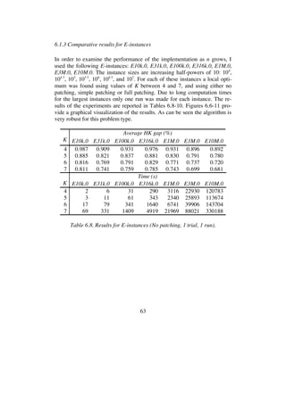
Download to read offline

![2
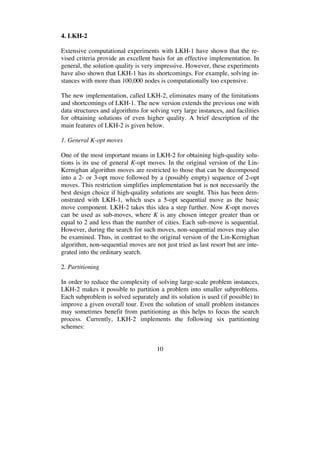
TSP may also be stated as the problem of finding a Hamiltonian cycle (tour)
of minimum weight in an edge-weighted graph:
Let G = (N, E) be a weighted graph where N = {1, 2, ..., n} is the set
of nodes and E = {(i, j) | i N, j N} is the set of edges. Each edge
(i, j) has associated a weight c(i, j). A cycle is a set of edges {(i1, i2),
(i2, i3), ..., (ik, i1)} with ip iq for p q. A Hamiltonian cycle (or tour)
is a cycle where k = n. The weight (or cost) of a tour T is the sum
(i, j) T c(i, j). An optimal tour is a tour of minimum weight.
For surveys of the problem and its applications, I refer the reader to the
excellent volumes edited by Lawler et al. [26] and Gutin and Punnen [13].
Local search with k-change neighborhoods, k-opt, is the most widely used
heuristic method for the traveling salesman problem. k-opt is a tour im-
provement algorithm, where in each step k links of the current tour are re-
placed by k links in such a way that a shorter tour is achieved.
It has been shown [8] that k-opt may take an exponential number of itera-
tions and that the ratio of the length of an optimal tour to the length of a tour
constructed by k-opt can be arbitrarily large when k n/2 - 5. Such undesir-
able cases, however, are very rare when solving practical instances [33].
Usually high-quality solutions are obtained in polynomial time. This is for
example the case for the Lin-Kernighan heuristic [26], one of the most ef-
fective methods for generating optimal or near-optimal solutions for the
symmetric traveling salesman problem. High-quality solutions are often
obtained, even though only a small part of the k-change neighborhood is
searched.
In the original version of the heuristic, the allowable k-changes (or k-opt
moves) are restricted to those that can be decomposed into a 2- or 3-change
followed by a (possibly empty) sequence of 2-changes. This restriction sim-
plifies implementation, but it need not be the best design choice. This report
explores the effect of widening the search.](https://image.slidesharecdn.com/koptreport-150110102502-conversion-gate01/85/Koptreport-2-320.jpg)
![3
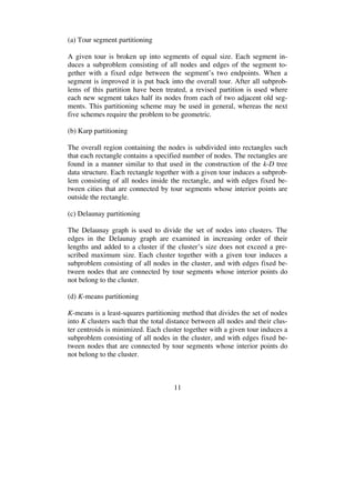
The report describes LKH-2, an implementation of the Lin-Kernighan heu-
ristic, which allows all those moves that can be decomposed into a sequence
of K-changes for any K where 2 K n. These K-changes may be sequen-
tial as well as non-sequential. LKH-2 is an extension and generalization of a
previous version, LKH-1 [18], which uses a 5-change as its basic move
component.
The rest of this report is organized as follows. Section 2 gives an overview
of the Lin-Kernighan algorithm. Section 3 gives a short description of the
first version of LKH, LKH-1. Section 4 presents the facilities of its succes-
sor LKH-2. Section 5 describes how general k-opt moves are implemented
in LKH-2. The effectiveness of the implementation is reported in Section 6.
The evaluation is based on extensive experiments for a wide variety of TSP
instances ranging from 10,000-city to 10,000,000-city instances. Finally, the
conclusions about the implementation are given in Section 7.](https://image.slidesharecdn.com/koptreport-150110102502-conversion-gate01/85/Koptreport-3-320.jpg)
![4
2. The Lin-Kernighan Algorithm
The Lin-Kernighan algorithm [27] belongs to the class of so-called local
search algorithms [19, 20, 22]. A local search algorithm starts at some lo-
cation in the search space and subsequently moves from the present location
to a neighboring location. The algorithm is specified in exchanges (or
moves) that can convert one candidate solution into another. Given a feasi-
ble TSP tour, the algorithm repeatedly performs exchanges that reduce the
length of the current tour, until a tour is reached for which no exchange
yields an improvement. This process may be repeated many times from ini-
tial tours generated in some randomized way.
The Lin-Kernighan algorithm (LK) performs so-called k-opt moves on tours.
A k-opt move changes a tour by replacing k edges from the tour by k edges
in such a way that a shorter tour is achieved. The algorithm is described in
more detail in the following.
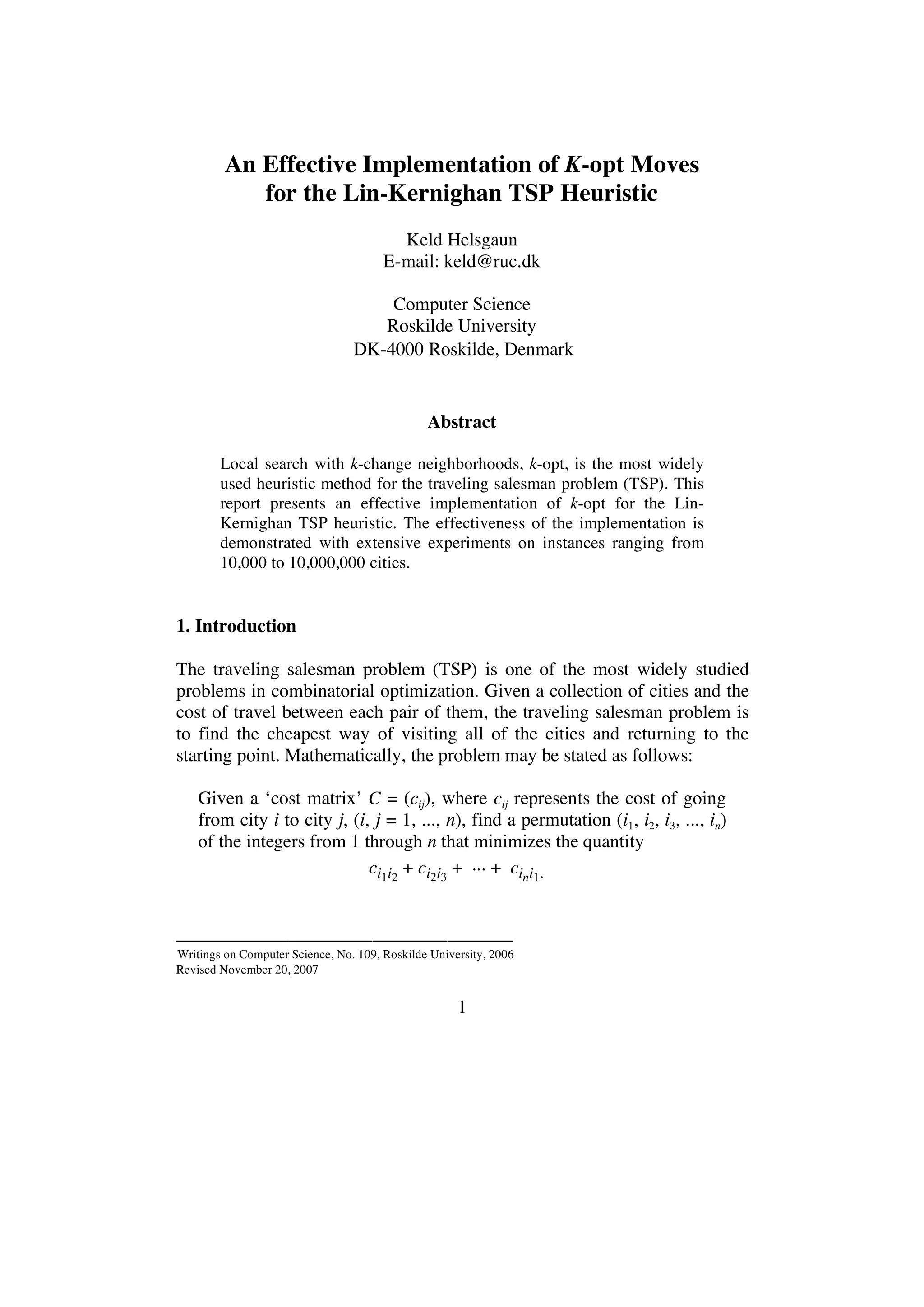
Let T be the current tour. At each iteration step the algorithm attempts to
find two sets of edges, X = {x1, ..., xk} and Y = {y1, ..., yk},, such that, if the
edges of X are deleted from T and replaced by the edges of Y, the result is a
better tour. The edges of X are called out-edges. The edges of Y are called
in-edges.
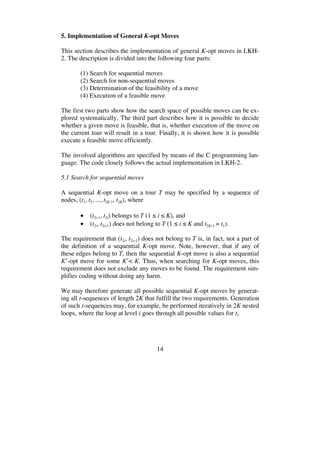
The two sets X and Y are constructed element by element. Initially X and Y
are empty. In step i a pair of edges, xi and yi, are added to X and Y, respec-
tively. Figure 2.1 illustrates a 3-opt move.
Figure 2.1. A 3-opt move.
x1, x2, x3 are replaced by y1, y2, y3.](https://image.slidesharecdn.com/koptreport-150110102502-conversion-gate01/85/Koptreport-4-320.jpg)


![8
3. The Modified Lin-Kernighan Algorithm (LKH-1)
Use of Lin and Kernighan’s original criteria, as described in the previous
section, results in a reasonably effective algorithm. Typical implementations
are able to find solutions that are 1-2% above optimum. However, in [18] it
was demonstrated that it was possible to obtain a much more effective im-
plementation by revising these criteria. This implementation, in the follow-
ing called LKH-1, made it possible to find optimum solutions with an im-
pressive high frequency. The revised criteria are described briefly below
(for details, see [18]).
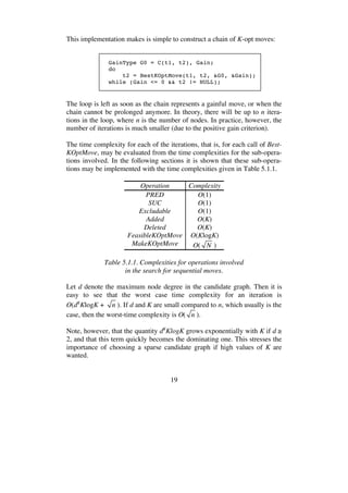
(1) The sequential exchange criterion
This criterion has been relaxed a little. When a tour can no longer be im-
proved by sequential moves, attempts are made to improve the tour by non-
sequential 4- and 5-opt moves.
(2) The feasibility criterion
A sequential 5-opt move is used as the basic sub-move. For i 1 it is re-
quired that x5i = (t10i-1,t10i), is chosen so that if t10i is joined to t1, the resulting
configuration is a tour. Thus, the moves considered by the algorithm are se-
quences of one or more 5-opt moves. However, the construction of a move
is stopped immediately if it is discovered that a close up to a tour results in a
tour improvement. Using a 5-opt move as the basic move instead of 2- or 3-
opt moves broadens the search and increases the algorithm’s ability to find
good tours, at the expense of an increase of running times.
(3) The positive gain criterion
This criterion has not been changed.
(4) The disjunctivity criterion
The sets X and Y need no longer be disjoint. In order to prevent an infinite
chain of sub-moves the following rule applies: The last edge to be deleted in
a 5-opt move must not previously have been added in the current chain of 5-
opt moves. Note that this relaxation of the criterion makes it possible to
generate certain non-sequential moves.](https://image.slidesharecdn.com/koptreport-150110102502-conversion-gate01/85/Koptreport-8-320.jpg)
![9
(5) The candidate set criterion
The usual measure for nearness, the costs of the edges, is replaced by a new
measure called the -measure. Given the cost of a minimum 1-tree [16, 17],
the -value of an edge is the increase of this cost when a minimum 1-tree is
required to contain the edge. The -values provide a good estimate of the
edges’ chances of belonging to an optimum tour. Using -nearness it is of-
ten possible to restrict the search to relative few of the -nearest neighbors
of a node, and still obtain optimal tours.](https://image.slidesharecdn.com/koptreport-150110102502-conversion-gate01/85/Koptreport-9-320.jpg)
![12
(e) Sierpinski partitioning
A tour induced by the Sierpinski spacefilling curve [34] is partitioned into
segments of equal size. Each of these segments together with a given tour
induces a subproblem. After all subproblems of this partition have been
treated, a revised partition of the Sierpinski tour is used where each new
segment takes half its nodes from each of two adjacent old segments.
(f) Rohe partitioning [35, 36]
Random rectangles are used to partition the node set into disjoint subsets of
about equal size. Each of these subsets together with a given tour induces a
subproblem.
3. Tour merging
LKH-2 provides a tour merging procedure that attempts to produce the best
possible tour from two or more given tours using local optimization on an
instance that includes all tour edges, and where edges common to the tours
are fixed. Tours that are close to optimum typically share many common
edges. Thus, the input graph for this instance is usually very sparse, which
makes it practicable to use K-opt moves for rather large values of K.
4. Iterative partial transcription
Iterative partial transcription is a general procedure for improving the per-
formance of a local search based heuristic algorithm. It attempts to improve
two individual solutions by replacing certain parts of either solution by the
related parts of the other solution. The procedure may be applied to the TSP
by searching for subchains of two tours, which contain the same cities in a
different order and have the same initial and final cities. LKH-2 uses the
procedure on each locally optimum tour and the current best tour. The
implemented algorithm is a simplified version of the algorithm described by
Möbius, Freisleben, Merz and Schreiber [31].
5. Backbone-guided search
The edges of the tours produced by a fixed number of initial trials may be
used as candidate edges in the succeeding trials. This algorithm, which is a
simplified version of the algorithm given by Zhang and Looks [38], has
proved particularly effective for VLSI instances.](https://image.slidesharecdn.com/koptreport-150110102502-conversion-gate01/85/Koptreport-12-320.jpg)

![15
Suppose the first element, t1, of the t-sequence has been selected. Then an
iterative algorithm for generating the remaining elements may be imple-
mented as shown in the pseudo code below.
for (each t[2] in {PRED(t[1]), SUC(t[1])}) {
G[0] = C(t[1], t[2]);
for (each candidate edge (t[2], t[3])) {
if (t[3] != PRED(t[2]) && t[3] != SUC(t[2]) &&
(G[1] = G[0] - C(t[2], t[3]) > 0) {
for (each t[4] in {PRED(t[3]), SUC(t[3])}) {
G[2] = G[1] + C(t[3], t[4]);
if (FeasibleKOptMove(2) &&
(Gain = G[2] - C(t[4], t[1])) > 0) {
MakeKOptMove(2);
return Gain;
}
}
inner loops for choosing t[5], ..., t[2K]
}
}
}
Comments:
• The t-sequence is stored in an array, t, of nodes. The three outermost
loops choose the elements t[2], t[3], and t[4]. The operations PRED
and SUC return for a given node respectively its predecessor and
successor on the tour,
• The function C(ta, tb), where ta and tb are two nodes, returns the cost
of the edge (ta, tb).
• The array G is used to store the accumulated gain. It is used for
checking that the positive gain criterion is fulfilled and for comput-
ing the gain of a feasible move.
• The function FeasibleKOptMove(k) determines whether a given t-se-
quence, (t1, t2, ..., t2k-1, t2k), represents a feasible k-opt move, where 2
≤ k ≤ K. The function MakeKOptMove(k) executes a feasible k-opt
move. The implementation of these functions is described in Sec-
tions 5.3 and 5.4.](https://image.slidesharecdn.com/koptreport-150110102502-conversion-gate01/85/Koptreport-15-320.jpg)
![16
• Note that, if during the search a gainful feasible move is discovered,
the move is executed immediately.
The inner loops for determination of t5, ..., t2K may be implemented analo-
gous to the code above. The innermost loop, however, has one extra task,
namely to register the non-gainful K-opt move that seems to be the most
promising one for continuing the chain of K-opt moves. The innermost loop
may be implemented as follows:
for (each t[2 * K] in {PRED(t[2 * K - 1], SUC[t[2 * K - 1]]}) {
G[2 * K] = G[2 * K - 1] + C(t[2 * K - 1], t[2 * K]);
if (FeasibleKOptMove(K)) {
if ((Gain = G[2 * K] - C(t[2 * K], t[1])) > 0) {
MakeKOptMove(K);
return Gain;
}
if (G[2 * K] > BestG2K &&
Excludable(t[2 * K - 1], t[2 * K])) {
BestG2K = G[2 * K];
for (i = 1; i <= 2 * K; i++)
Best_t[i] = t[i];
}
}
}
Comments:
• The feasible K-opt move that maximizes the cumulative gain,
G[2K], is considered to be the most promising move.
• The function Excludable is used to examine whether the last edge to
be deleted in a K-opt move has previously been added in the current
chain of K-opt moves (Criterion 4 in Section 3).
Generation of 5-opt moves in LKH-1 was implemented as described above.
However, if we want to generate K-opt moves, where K may be chosen
freely, this approach is not appropriate. In this case we would like to use a
variable number of nested loops. This is normally not possible in imperative
languages like C, but it is well known that it may be simulated by use of re-
cursion. A recursive implementation of the algorithm is given below.](https://image.slidesharecdn.com/koptreport-150110102502-conversion-gate01/85/Koptreport-16-320.jpg)
![17
GainType BestKOptMoveRec(int k, GainType G0) {
GainType G1, G2, G3, Gain;
Node *t1 = t[1], *t2 = t[2 * k - 2], *t3, *t4;
int i;
for (each candidate edge (t2, t3)) {
if (t3 != PRED(t2) && t3 != SUC(t2) &&
!Added(t2, t3, k - 2) &&
(G1 = G0 – C(t2, t3)) > 0) {
t[2 * k - 1] = t3;
for (each t4 in {PRED(t3), SUC(t3)}) {
if (!Deleted(t3, t4, k - 2)) {
t[2 * k] = t4;
G2 = G1 + C(t3, t4);
if (FeasibleKOptMove(k) &&
(Gain = G2 - C(t4, t1)) > 0) {
MakeKOptMove(k);
return Gain;
}
if (k < K &&
(Gain = BestKOptMoveRec(k + 1, G2)) > 0)
return Gain;
if (k == K && G2 > BestG2K &&
Excludable(t3, t4)) {
BestG2K = G2;
for (i = 1; i <= 2 * K; i++)
Best_t[i] = t[i];
}
}
}
}
}
}
Comment:
• The auxiliary functions Added and Deleted are used to ensure that no
edge is added or deleted more than once in the move under con-
struction. Possible implementations of the two functions are shown
below. It is easy to see that the time complexity for each of these
functions is O(k).](https://image.slidesharecdn.com/koptreport-150110102502-conversion-gate01/85/Koptreport-17-320.jpg)
![18
int Added(Node *ta, Node *tb, int k) {
int i = 2 * k;
while ((i -= 2) > 0)
if ((ta == t[i] && tb == t[i + 1]) ||
(ta == t[i + 1] && tb == t[i]))
return 1;
return 0;
}
int Deleted(Node * ta, Node * tb, int k) {
int i = 2 * k + 2;
while ((i -= 2) > 0)
if ((ta == t[i - 1] && tb == t[i]) ||
(ta == t[i] && tb == t[i - 1]))
return 1;
return 0;
}
Given two neighboring nodes on the tour, t1 and t2, the search for a K-opt
move is initiated by a call of the driver function BestKOptMove shown be-
low.
Node *BestKOptMove(Node *t1, Node *t2,
GainType *G0, GainType *Gain) {
t[1] = t1; t[2] = t2;
BestG2K = MINUS_INFINITY;
Best_t[2 * K] = NULL;
*Gain = BestKOptMoveRec(2, *G0);
if (*Gain <= 0 && Best_t[2 * K] != NULL) {
for (i = 1; i <= 2 * K; i++)
t[i] = Best_t[i];
MakeKOptMove(K);
}
return Best_t[2 * K];
}](https://image.slidesharecdn.com/koptreport-150110102502-conversion-gate01/85/Koptreport-18-320.jpg)

![22
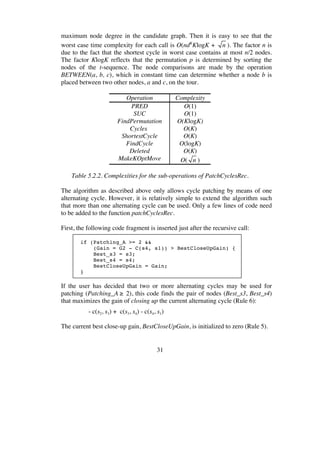
Figure 5.2.3 illustrates that it is also possible to use three alternating cycles:
(s1, s2, s3, s4, s6), (t1, t2, t3, t4, t1), and (u1, u2, u3, u4, u1). In general, K cycles
may be transformed into a tour using up to K-1 alternating cycles.
Figure 5.2.3. Four disjoint cycles patched by three alternating cycles.
With the addition of non-sequential moves, the number of different types of
k-opt moves that the algorithm must be able to handle has increased consid-
erably. In the following this statement is quantified.
Let MT(k) denote the number of k-opt move types. A k-opt move removes k
edges from a tour and adds k edges that reconnect k tour segments into a
tour. Hence, a k-opt move may be defined as a cyclic permutation of k tour
segments where some of the segments may be inverted (swapped). Let one
of the segments be fixed. Then MT(k) can be computed as the product of the
number of inversions of k-1 segments and the number of permutations of
k-1 segments:
MT(k) = 2k 1
(k 1)!.
However, MT(k) includes the number of moves, which reinserts one or more
of the deleted edges. Since such moves may be generated by k’-opt moves
where k’< k, we are more interested in computing PMT(k), the number of
pure k-opt moves, that is, moves for which the set of removed edges and the
set of added edges are disjoint. Funke, Grünert and Irnich [11, p. 284] give
the following recursion formula for PMT(k):](https://image.slidesharecdn.com/koptreport-150110102502-conversion-gate01/85/Koptreport-22-320.jpg)
![23
PMT(k) = MT(k) − i
k
( )
i=2
k−1
∑ PMT(i) −1 for k ≥ 3
PMT(2) = 1
An explicit formula for PMT(k) may be derived from the formula for series
A061714 in The On-Line Encyclopedia of Integer Sequences [40]:
PMT(k) = (−1)k+ j−1
j=0
i
∑
i=1
k−1
∑ j
i
( )j!2j
for k ≥ 2
The set of pure moves accounts for both sequential and non-sequential
moves. To examine how much the search space has been enlarged by the
inclusion of non-sequential moves, we will compute SPMT(k), the number
of sequential, pure k-opt moves, and compare this number with the PMT(k).
The explicit formula for SPMT(k) shown below has been derived by Han-
lon, Stanley and Stembridge [14]:
SPMT(k) =
23k−2
k!(k −1)!2
(2k)!
+ ca,b (2)
b=1
min(a,k−a)
∑
a=1
k−1
∑
2a−b−1
(2b)!(a −1)!(k − a − b −1)
(2b −1)b!
⎡
⎣
⎢
⎤
⎦
⎥
2
where
ca,b (2) =
(−1)k (−2)a−b+1
k(2a − 2b +1)(a −1)!
(k + a − b +1)(k + a − b)(k − a + b)(k − a + b −1)(k − a − b)!(2a −1)!(b −1)!
Table 5.2.1 depicts MT(k), PMT(k), SPMT(k), and the ratio SPMT(k)/MPT(k)
for selected values of k. As seen, the ratio SMPT(k)/PMT(k) decreases as k
increases. For k ≥ 10, there are fewer types of sequential moves than types of
non-sequential moves.
k 2 3 4 5 6 7 8 9 10 50 100
MT(k) 2 8 48 384 3840 46080 645120 1.0E7 1.9E8 3.4E77 5.9E185
PMT(k) 1 4 25 208 2121 25828 365457 5.9E6 1.1E8 2.1E77 3.6E185
SPMT(k) 1 4 20 148 1348 15104 198144 3.0E6 5.1E7 4.3E76 5.9E184
SPMT (k)
PMT (k) 1 1 0.80 0.71 0.63 0.58 0.54 0.51 0.48 0.21 0.17
Table 5.2.1. Growth of move types for k-opt moves.](https://image.slidesharecdn.com/koptreport-150110102502-conversion-gate01/85/Koptreport-23-320.jpg)

![26
GainType PatchCycles(int k, GainType Gain) {
Node *s1, *s2, *sStart, *sStop;
GainType NewGain;
int M, i;
FindPermutation(k);
M = Cycles(k);
if (M == 1 || M > Patching_C)
return 0;
CurrentCycle = ShortestCycle(M, k);
for (i = 0; i < k; i++) {
if (cycle[p[2 * i]] == CurrentCycle) {
sStart = t[p[2 * i]];
sStop = t[p[2 * i + 1]];
for (s1 = sStart; s1 != sStop; s1 = s2) {
t[2 * k + 1] = s1;
t[2 * k + 2] = s2 = SUC(s1);
if ((NewGain =
PatchCyclesRec(k, 2, M,
Gain + C(s1, s2))) > 0)
return NewGain;
}
}
}
return 0;
}
Comments:
• The function is called from the inner loop of BestKOptMoveRec:
if (t4 != t1 && Patching_C >= 2 &&
(Gain = G2 - C(t4, t1)) > 0 && // rule 5
(Gain = PatchCycles(k, Gain)) > 0)
return Gain;
• The parameter k specifies that, given the non-feasible k-opt move
represented by the nodes in the global array t[1..2k], the function
should try to find a gainful feasible move by cycle patching. The
parameter Gain specifies the gain of the non-feasible input move.](https://image.slidesharecdn.com/koptreport-150110102502-conversion-gate01/85/Koptreport-26-320.jpg)
![27
• We need to be able to traverse those nodes that belong to the small-
est cycle component (Rule 4), and for a given node to determine
quickly to which of the current cycles it belongs to (Rule 3). For that
purpose we first determine the permutation p corresponding to the
order in which the nodes in t[1..2k] occur on the tour in a clockwise
direction, starting with t[1]. For example, p = (1 2 4 3 9 10 7 8 5 6)
for the non-feasible 5-opt move shown in Figure 5.2.4. Next, the
function Cycles is called to determine the number of cycles and to
associate with each node in t[1..2k] the number of the cycle it be-
longs to. Execution of the 5-opt in Figure 5.2.4 move produces two
cycles, one represented by the node sequence (t1, t10, t7, t6, t1), and
one represented by the node sequence (t2, t4, t5, t8, t9, t3, t2). The nodes
of the first sequence are labeled with 1, the nodes of the second se-
quence with 2.
Figure 5.2.4. Non-feasible 5-opt move (2 cycles).
Next, the function ShortestCycle (shown below) is called in order to
find the shortest cycle. The function returns the number of the cycle
that contains the lowest number of nodes.](https://image.slidesharecdn.com/koptreport-150110102502-conversion-gate01/85/Koptreport-27-320.jpg)
![28
int ShortestCycle(int M, int k) {
int i, MinCycle, MinSize = INT_MAX;
for (i = 1; i <= M; i++)
size[i] = 0;
p[0] = p[2 * k];
for (i = 0; i < 2 * k; i += 2)
size[cycle[p[i]]] +=
SegmentSize(t[p[i]], t[p[i + 1]]);
for (i = 1; i <= M; i++) {
if (size[i] < MinSize) {
MinSize = size[i];
MinCycle = i;
}
}
return MinCycle;
}
• The tour segments of the shortest cycle are traversed by exploiting
the fact that t[p[2i]] and t[p[2i + 1]] are the two end points for a tour
segment of a cycle, for 0 i < k and p[0] = p[2k]. Which cycle a
tour segment is part of may be determined simply by retrieving the
cycle number associated with one of its two end points.
• Each tour edge of the shortest cycle may now be used as the first
out-edge, (s1, s2), of an alternating cycle. An alternating cycle is con-
structed by the recursive function PatchCyclesRec shown below.](https://image.slidesharecdn.com/koptreport-150110102502-conversion-gate01/85/Koptreport-28-320.jpg)
![29
GainType PatchCyclesRec(int k, int m, int M, GainType G0) {
Node *s1, *s2, *s3, *s4;
GainType G1, G2, G3, G4, Gain;
int NewCycle, cycleSaved[1 + 2 * k], i;
s1 = t[2 * k + 1];
s2 = t[i = 2 * (k + m) - 2];
incl[incl[i] = i + 1] = i;
for (i = 1; i <= 2 * k; i++)
cycleSaved[i] = cycle[i];
for (each candidate edge (s2, s3)) {
if (s2 != PRED(s2) && s3 != SUC(s2) &&
(NewCycle = FindCycle(s3, k)) != CurrentCycle) {
t[2 * (k + m) - 1] = s3;
G1 = G0 – C(s2, s3);
for (each s4 in {PRED(s3), SUC(s3)}) {
if (!Deleted(s3, s4, k)) {
t[2 * (k + m)] = s4;
G2 = G1 + C(s3, s4);
if (M > 2) {
for (i = 1; i <= 2 * k; i++)
if (cycle[i] == NewCycle)
cycle[i] = CurrentCycle;
if ((Gain =
PatchCyclesRec(k, m + 1, M - 1,
G2)) > 0)
return Gain;
for (i = 1; i <= 2 * k; i++)
cycle[i]= cycleSaved[i];
} else if (s4 != s1 &&
(Gain = G2 – C(s4, s1)) > 0) {
incl[incl[2 * k + 1] = 2 * (k + m)] =
2 * k + 1;
MakeKOptMove(k + m);
return Gain;
}
}
}
}
}
return 0;
}](https://image.slidesharecdn.com/koptreport-150110102502-conversion-gate01/85/Koptreport-29-320.jpg)
![30
Comments:
• The algorithm is rather simple and very much resembles the Best-
KOptMoveRec function. The parameter k is used to specify that a non-
feasible k-opt move be used as the starting point for finding a gainful fea-
sible move. The parameter m specifies the current number of out-edges of
the alternating cycle under construction. The parameter M specifies the
current number of cycle components (M 2). The last parameter, G0,
specifies the accumulated gain.
• If a gainful feasible move is found, then this move is executed by calling
MakeKOptMove(k + m) before the achieved gain is returned.
• A move is represented by the nodes in the global array t, where the first
2k elements are the nodes of the given non-feasible sequential k-opt
move, and the subsequent elements are the nodes of the alternating cycle.
In order to be able to determine quickly whether an edge is an in-edge or
an out-edge of the current move we maintain an array, incl, such that
incl[i] = j and incl[j] = i is true if and only if the edge (t[i], t[j]) is an in-
edge. For example, in Figure 5.2.4 incl = [10, 3, 2, 5, 4, 7, 6, 9, 8, 1]. It is
easy to see that there is no reason to maintain similar information about
out-edges as they always are those edges (t[i], t[i + 1]) for which i is odd.
• Let s2 be the last node added to the t-sequence. At each recursive call of
PatchCyclesRec the t-sequence is extended by two nodes, s3 and s4, such
that
(a) (s2, s3) is a candidate edge,
(b) s3 belongs to a not yet visited cycle component,
(c) s4 is a neighbor to s3 on the tour, and
(d) the edge (s3, s4) has not been deleted before.
• Before a recursive call of the function all cycle numbers of those nodes of
t[1..2k] that belong to s3’s cycle component are changed to the number of
the current cycle component (which is equal to the number of s2’s cycle
component).
The time complexity for a call of PatchCyclesRec may be evaluated from the
time complexities for the sub-operations involved. The sub-operations may be
implemented with the time complexities given in Table 5.2.2. Let d denote the](https://image.slidesharecdn.com/koptreport-150110102502-conversion-gate01/85/Koptreport-30-320.jpg)
![32
Second, the last statement of PatchCyclesRec (the return statement) is replaced
by the following code:
Gain = 0;
if (BestCloseUpGain > 0) {
int OldCycle = CurrentCycle;
t[2 * (k + m) - 1] = Best_s3;
t[2 * (k + m)] = Best_s4;
Patching_A--;
Gain = PatchCycles(k + m, BestCloseUpGain);
Patching_A++;
for (i = 1; i <= 2 * k; i++)
cycle[i]= cycleSaved[i];
CurrentCycle = OldCycle;
}
return Gain;
Note that this causes a recursive call of PatchCycles (not PatchCyclesRec).
The algorithm described in this section is somewhat simplified in relation to the
algorithm implemented in LKH-2. For example, when two cycles arise, LKH-2
will attempt to patch them, not only by means of an alternating cycle consisting
of 4 edges (a 2-opt move), but also by means of an alternating cycle consisting of
6 edges (a 3-opt move).](https://image.slidesharecdn.com/koptreport-150110102502-conversion-gate01/85/Koptreport-32-320.jpg)

![34
way. For example, if we start in node t6 in Figure 5.3.1a, and jump from t-
node to t-node following the direction of the arrows, then all t-nodes are
visited in the following sequence: t6, t7, t6, t5, t4, t2, t3, t8, t1.
It is easy to jump from one t-node, ta, to another, tb, if the edge (ta, tb) is an
in-edge. We only need to maintain an array, incl, which represents the cur-
rent in-edges. If (ta, tb) is an in-edge for a k-opt move (1 a,b 2k), this fact
is registered in the array by setting incl[a] = b and incl[b] = a. By this means
each such jump can be made in constant time (by a table lookup).
On the other hand, it is not obvious how we can skip those nodes that are
not t-nodes. It turns out that a little preprocessing solves the problem. If we
know the cyclic order in which the t-nodes occur on the original tour, then it
becomes easy to skip all nodes that lie between two t-nodes on the tour. For
a given t-node we just have to select either its predecessor or its successor in
this cyclic ordering. Which of the two cases we should choose can be de-
termined in constant time. This kind of jump may therefore be made in con-
stant time if the t-nodes have been sorted. I will now show that this sorting
can be done in O(klogk) time.
First, we realize that is not necessary to sort all t-nodes. We can restrict our-
selves to sorting half of the nodes, namely for each out-edge the first end
point met when the tour is traversed in a given direction. If in Figure 5.3.1
the chosen direction is “clockwise”, we may restrict the sorting to the four
nodes t1, t4, t5, and t8. If the result of a sorting is represented by a permuta-
tion, phalf, then phalf will be equal to (1 4 8 5). This permutation may easily be
extended to a full permutation containing all node indices, p = (1 2 4 3 8 7 5
6). The missing node indices are inserted by using the following rule: if
phalf[i] is odd, then insert phalf[i] + 1 after phalf[i], otherwise insert phalf[i] - 1
after phalf[i].
Let a move be represented by the nodes t[1..2k]. Then the function Find-
Permutation shown below is able to find the permutation p[1..2k] that corre-
sponds to their visiting order when the tour is traversed in the SUC-direc-
tion. In addition, the function determines q[1..2k] as the inverse permutation
to p, that is, the permutation for which q[p[i]] = i for 1 i 2k.](https://image.slidesharecdn.com/koptreport-150110102502-conversion-gate01/85/Koptreport-34-320.jpg)
![35
void FindPermutation(int k) {
int i,j;
for (i = j = 1; j <= k; i += 2, j++)
p[j] = (SUC(t[i]) == t[i + 1]) ? i : i + 1;
qsort(p + 2, k - 1, sizeof(int), Compare);
for (j = 2 * k; j >= 2; j -= 2) {
p[j - 1] = i = p[j / 2];
p[j] = i & 1 ? i + 1 : i - 1;
}
for (i = 1; i <= 2 * k; i++)
q[p[i]] = i;
}
Comments:
• First, the k indices to be sorted are placed in p. This takes O(k) time.
Next, the sorting is performed. The first element of p, p[1] is fixed
and does not take part in the sorting. Thus, only k-1 elements are
sorted. The sorting is performed by C’s library function for sorting,
qsort, using the comparison function shown below:
int Compare(const void *pa, const void *pb) {
return BETWEEN(t[p[1]], t[*(int *) pa], t[*(int *) pb])
? -1 : 1;
}
The operation BETWEEN(a, b, c) determines in constant time
whether node b lies between node a and node c on the tour in the
SUC-direction. Since the number of comparisons made by qsort on
average is O(klogk), and each comparison takes constant time, the
sorting process takes O(klogk) time on average.
• After the sorting, the full permutation, p, and its inverse, q, are built.
This can be done in O(k) time.
• From the analysis above we find that the average time for calling
FindPermutation with argument k is O(klogk).](https://image.slidesharecdn.com/koptreport-150110102502-conversion-gate01/85/Koptreport-35-320.jpg)
![36
After having determined p and q, we can quickly determine whether a k-opt
move represented by the contents of the arrays t and incl is feasible. The
function shown below shows how this can be achieved.
int FeasibleKOptMove(int k) {
int Count = 1, i = 2 * k;
FindPermutation(k);
while ((i = q[incl[p[i]]] ^ 1) != 0)
Count++;
return (Count == k);
}
Comments:
• In each iteration of the while-loop the two end nodes of an in-edge
are visited, namely t[p[i]] and t[incl[p[i]]]. The inverse permutation,
q, makes it possible to skip possible t-nodes between t[incl[p[i]]] and
the next t-node on the cycle. If the position of incl[p[i]] in p is even,
then in the next iteration i should be equal to this position plus one.
Otherwise, it should be equal to this position minus one.
• The starting value for i is 2k. The loop terminates when i becomes
zero, which happens when node t[p[1]] has been visited (since 1 ^ 1
= 0, where ^ is the exclusive OR operator). The loop always termi-
nates since both t[p[2k]] and t[p[1]] belong to the cycle that is tra-
versed by the loop, and no node is visited more than once.
• It is easy to see that the loop is executed in O(k) time. Since the sort-
ing made by the call of FindPermutation on average takes O(klogk)
time, we can conclude that the average-time complexity for the
FeasibleKOptMove function is O(klogk). Normally, k is very small
compared to the total number of nodes, n. Thus, we have obtained an
algorithm that is efficient in practice.
• To see a concrete example of how the algorithm works, consider the
4-opt move in Figure 5.3.1a. Before the while-loop the following is
true:
p = (1 2 4 3 8 7 5 6)
q = (1 2 4 3 7 8 6 5)
incl = (8 3 2 5 4 7 6 1)](https://image.slidesharecdn.com/koptreport-150110102502-conversion-gate01/85/Koptreport-36-320.jpg)

![38
5.4 Execution of a feasible move
In order to simplify execution of a feasible k-opt move, the following fact
may be used: Any k-opt move (k 2) is equivalent to a finite sequence of 2-
opt moves [9, 28]. In the case of 5-opt moves it can be shown that any 5-opt
move is equivalent to a sequence of at most five 2-opt moves. Any 3-opt
move as well as any 4-opt move is equivalent to a sequence of at most three
2-opt moves. In general, any feasible k-opt move may be executed by at
most k 2-opt moves. For a proof, see [30].
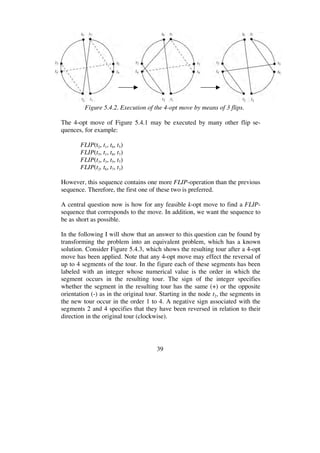
Let FLIP(a, b, c, d) denote the operation of replacing the two edges (a, b)
and (c, d) of the tour by the two edges (b, c) and (d, a). Then the 4-opt move
depicted in Figure 5.4.1 may be executed by the following sequence of
FLIP-operations:
FLIP(t2, t1, t8, t7)
FLIP(t4, t3, t2, t7)
FLIP(t7, t4, t5, t6)
The execution of the flips is illustrated in Figure 5.4.2.
Figure 5.4.1. Feasible 4-opt move.](https://image.slidesharecdn.com/koptreport-150110102502-conversion-gate01/85/Koptreport-38-320.jpg)

![42
It is easy to see that determination of a shortest possible FLIP-sequence for a
k-opt move is a SSBR problem. We are therefore interested in finding an
efficient algorithm for solving SSBR. It is known that the unsigned version,
SBR, is NP-hard [7], but, fortunately, the signed version, SSBR, has been
shown to be polynomial by Hannenhalli and Pevzner in 1995, and they gave
an algorithm for solving the problem in O(n4
) time [15]. Since then faster
algorithms have been discovered, among others an O(n2
) algorithm by Kap-
lan, Shamir and Tarjan [25]. The fastest algorithm for SSBR today has com-
plexityO(n nlogn) [37].
Several of these fast algorithms are difficult to implement. I have chosen to
implement a very simple algorithm described by Bergeron [6]. The algo-
rithm has a worst-time complexity of O(n3
). However, as it on average runs
in O(n2
) time, and hence in O(k2
) for a k-opt move, the algorithm is sufficient
efficient for our purpose. If we assume k << n, where n is the number of cit-
ies, the time for determining the minimal flip sequence is dominated by the
time to make the flips, O( n) .
Before describing Bergeron’s algorithm and its implementation, some neces-
sary definitions are stated [6].
Let = ( 1 ..., n) be a signed permutation. An oriented pair ( i, j) is a pair
of adjacent integers, that is | i| - | j| = ±1, with opposite signs. For example,
the signed permutation
(+1 -2 -5 +4 +3)
contains three oriented pairs: (+1, -2), (-2, +3), and (-5, +4).
Oriented pairs are useful as they indicate reversals that cause adjacent inte-
gers to be consecutive in the resulting permutation. For example, the ori-
ented pair (-2, +3) induces the reversal
(+1 -2 -5 +4 +3) (+1 -4 +5 +2 +3)
creating a permutation where +3 is consecutive to +2.](https://image.slidesharecdn.com/koptreport-150110102502-conversion-gate01/85/Koptreport-42-320.jpg)

![44
Thus, if we want a minimum number of reversals, we have to be careful in
selecting the initial reversal in this case.
A possible strategy for selecting this reversal is the following.
Algorithm 2:
Find the pair (+ i, + j) for which | j – i| = 1, j i + 3, and i is minimal.
Then reverse the segment (+ i+1 ... + j-1).
In the example above, the pair (+1, +2) is found, and the segment (+4 +3) is
reversed. In this example, this strategy is sufficient to sort the permutation
optimally. However, we cannot be sure that this is always the case. If, for
example, a permutation is sorted in reversed order, (+n ... +2 +1), there is no
pair that fulfills the conditions above. However, this situation can be avoided
by requiring that +1 is always the first element of a permutation. Unless the
permutation is sorted, we are always able to find a pair that satisfies the con-
dition.
It is easy to see that this strategy is sufficient to sort any permutation. When
a positive permutation is created, we select the first pair (+ i, + j) for which
+ i is in its correct position, and + j is not. When the segment between these
two elements is reversed, at least one oriented pair is created. After making
the reversal induced by this oriented pair, the sign of + j is reversed, so that a
subsequent reversal can bring + j to its correct position (right after + i).
The question now is whether the strategy is optimal. To answer this ques-
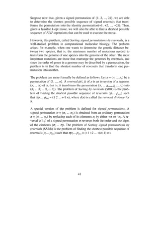
tion, we will use the notion of a cycle graph of a permutation [5]. Let be a
signed permutation. The first step in constructing the cycle graph is to frame
by the two extra elements 0 and n + 1: = (0 1 2 ... n n+1). Next, this
permutation is mapped one-to-one into an unsigned permutation ’ of 2n+2
elements by replacing
• each positive element +x in by the sequence 2x-1 2x,
• each negative element -x in by the sequence 2x 2x+1, and
• n+1 by 2n-1.](https://image.slidesharecdn.com/koptreport-150110102502-conversion-gate01/85/Koptreport-44-320.jpg)
![45
For example, the permutation
= (+1 -4 -2 +3 5)
becomes
’ = (0 1 2 8 7 4 3 5 6 9)
Note that the mapping is one-to-one. The reversal (i, j) of corresponds to
the reversal (2i-1, 2j) of ’.
The cycle graph for is an edge-colored graph of 2n+2 nodes { 0 1 ...
2n+2}. For each i, 0 i n, we join two nodes 2i and 2i+1 by a black edge,
and with a gray edge, if | 2i+1 - 2i| = 1. Figure 5.4.4 depicts an example of a
cycle graph. Black edges appear as straight lines. Gray edges appear as
curved lines.
Figure 5.4.4. Cycle graph for = (+1 -4 -2 +3).
The black edges are called reality edges, and the gray edges are called dream
edges [37]. The reality edges define the permutation ’ (what you have), and
the dream edges define the identity permutation (what you want).
Every node has degree two, that is, every node has exactly two incident
edges. Thus a cycle graph consists of a set of cycles. Each of these cycles is
an alternating cycle, that is, adjacent edges have different colors.
We use k-cycle to refer to an alternating cycle of length k, that is, a cycle
consisting of k edges. The cycle graph in Figure 5.5.4 consists of a 2-cycle
and an 8-cycle. The cycle graph for the identity permutation (+1 +2 ... +n)
consists of n+1 2-cycles (see Figure 5.4.5). Sorting by reversals can be
viewed as a process that increases the number of cycles to n + 1.](https://image.slidesharecdn.com/koptreport-150110102502-conversion-gate01/85/Koptreport-45-320.jpg)
![46
Figure 5.4.5. Cycle graph for = (+1 +2 +3 +4).
It is easy to see that every reversal induced by an ordered pair increases the
number of cycles by one. On the other hand, if there is no ordered pair (be-
cause the permutation is positive), then there is no single reversal, which will
increase the number of cycles. In this case we will try to find a reversal,
which without reducing the number of cycles creates one or more oriented
pairs.
A cycle is said to be oriented if it contains edges that correspond to one or
more oriented pairs; otherwise, it is said to be non-oriented. We must, as far
as possible, avoid creating non-oriented cycles, unless they are 2-cycles.
Let be positive permutation, and assume that is reduced, that is, does
not contain consecutive elements. A framed interval in is an interval of the
form
i j+1 j+2 ... j+k-1 i+k
such that all its elements belong to the interval [i ... i+k]. In other words, a
framed interval consists of integers that can be reordered as i i+1 ... i+k.
Keep in mind that since is a circular permutation, we may wrap around
from the end to the start. Consider the permutation below (the plus signs
have been omitted):
(1 4 7 6 5 8 3 2 9)
The whole permutation is a framed interval. The segment 4 7 6 5 8 is a
framed interval, and the segment 3 2 9 1 4 is also a framed interval, since, by
circularity, 1 is the successor of 9, and the permutation can be reordered as
9 1 2 3 4.](https://image.slidesharecdn.com/koptreport-150110102502-conversion-gate01/85/Koptreport-46-320.jpg)
![47
Now we can conveniently define a hurdle. A hurdle is a framed interval that
does not contain any shorter framed intervals. In the example above, the
whole permutation is not a hurdle, since it contains the framed interval 4 7 6
5 8. The framed intervals 4 7 6 5 8 and 3 2 9 1 4 are both hurdles, since they
do not properly contain any framed intervals.
In order to get rid of hurdles, two operations are introduced: hurdle cutting
and hurdle merging. The first one, hurdle cutting, consists in reversing the
segment between i and i + 1 of a hurdle:
i j+1 j+2 ... i+1... j+k-1 i+k
Given the permutation (1 4 7 6 5 8 3 2 9), the result of cutting the hurdle 4 7
6 5 8 is the permutation (1 4 -6 -7 5 8 3 2 9).
It has been shown that when a permutation contains only one hurdle, one
such reversal creates enough oriented pairs to completely sort the resulting
permutation by means of oriented reversals. However, when a permutation
contains two or more hurdles, this is not always the case. We need one more
operation: hurdle merging.
Hurdle merging consists of reversing the segment between two end points of
two hurdles, inclusive the two end points:
i j+1 j+2 ... i+k ... i’ ... i+k
It has been shown [15] that the following algorithm, together with Algorithm
1, can be used to optimally sort any signed permutation:
Algorithm 3:
If a permutation has an even number of hurdles, merge two con-
secutive hurdles. If a permutation has an odd number of hurdles,
then if it has one hurdle whose cutting decreases the number of
cycles, then cut it; otherwise, merge two non-consecutive hurdles,
or consecutive hurdles if there are exactly three hurdles.](https://image.slidesharecdn.com/koptreport-150110102502-conversion-gate01/85/Koptreport-47-320.jpg)
![49
Below is given a function, MakeKOptMove, which uses these algorithms for
executing a k-opt move using a minimum number of FLIP-operations.
void MakeKOptMove(long k) {
int i, j, Best_i, Best_j, BestScore, s;
FindPermutation(k);
FindNextReversal:
BestScore = -1;
for (i = 1; i <= 2 * k - 2; i++) {
j = q[incl[p[i]]];
if (j >= i + 2 && (i & 1) == (j & 1) &&
(s = (i & 1) == 1 ? Score(i + 1, j, k) :
Score(i, j - 1, k)) > BestScore) {
BestScore = s; Best_i = i; Best_j = j;
}
}
if (BestScore >= 0) {
i = Best_i; j = Best_j;
if ((i & 1) == 1) {
FLIP(t[p[i + 1]], t[p[i]], t[p[j]], t[p[j + 1]]);
Reverse(i + 1, j);
} else {
FLIP(t[p[i - 1]], t[p[i]], t[p[j]], t[p[j - 1]]);
Reverse(i, j - 1);
}
goto FindNextReversal;
}
for (i = 1; i <= 2 * k - 1; i += 2) {
j = q[incl[p[i]]];
if (j >= i + 2) {
FLIP(t[p[i]], t[p[i + 1]], t[p[j]], t[p[j - 1]]);
Reverse(i + 1, j - 1);
goto FindNextReversal;
}
}
}
Comments:
• At entry the move to be executed must be available in the two global
arrays t and incl, where t contains the nodes of the alternating cycles,
and incl represents the in-edges of these cycles, {(t[i], t[incl[i]]) :
1 ≤ i ≤ 2k}.](https://image.slidesharecdn.com/koptreport-150110102502-conversion-gate01/85/Koptreport-49-320.jpg)
![50
• First, the function FindPermutation is called in order to find the per-
mutation p and its inverse q, where p gives the order in which the t-
nodes occur on the tour (see Section 5.3).
• The first for-loop determines, if possible, an oriented reversal with
maximum score. At each iteration, the algorithm explores the two
cases shown in Figures 5.4.8 and 5.4.9.
Figure 5.4.8. Oriented reversal: j i+2 i odd j odd p[j] = incl[p[i]].
Figure 5.4.9. Oriented reversal: j i +2 i even j even p[j] =
incl[p[i]].
• If an oriented reversal is found, it is executed. Otherwise, the last for-
loop of the algorithm searches for a non-oriented reversal (caused by
a hurdle). See Figure 5.4.10.
Figure 5.4.10 Non-oriented reversal: j i +3 i odd j even p[j] =
incl[p[i]].
• As soon as a reversal has been found, the reversal and the
corresponding FLIP-operation on the tour are executed. The fourth
argument of FLIP has been omitted, as it can be computed from the
first three. The auxiliary function Reverse, shown below, executes a
reversal of the permutation segment p[i..j] and updates the inverse
permutation q accordingly.](https://image.slidesharecdn.com/koptreport-150110102502-conversion-gate01/85/Koptreport-50-320.jpg)
![51
void Reverse(int i, int j) {
for (; i < j; i++, j--) {
int pi = p[i];
q[p[i] = p[j]] = i;
q[p[j] = pi] = j;
}
}
• The auxiliary function Score, shown below, returns the score of the
reversal of p[left..right].
int Score(int left, int right, int k) {
int count = 0, i, j;
Reverse(left, right);
for (i = 1; i <= 2 * k - 2; i++) {
j = q[incl[p[i]]];
if (j >= i + 2 && (i & 1) == (j & 1))
count++;
}
Reverse(left, right);
return count;
}
Since the tour is represented by the two-level tree data structure [10], the
complexity of the FLIP-operation isO( N ). The complexity of Make-
KOptMove is O(k N + k3
), since there are at most k calls of FLIP, and at
most k2
calls of Score, each of which has complexity O(k).
The complexity of Score may be reduced from O(k) to O(logk) by using a
balanced search tree [12]. This will reduce the complexity of Make-
KOptMove to O(k n + k2
logk). However, this is of little practical value,
since usually k is very small in relation to n, so that the term k n domi-
nates.
The presented algorithm for executing a move minimizes the number of
flips. However, this need not be the best way to minimize running time. The
lengths of the tour segments to be flipped should not be ignored. Currently,
however, no algorithm is known that solves this sorting problem optimally.
It is an interesting area of future research.](https://image.slidesharecdn.com/koptreport-150110102502-conversion-gate01/85/Koptreport-51-320.jpg)
![52
6. Computational Results
This section presents the results of a series of computational experiments,
the purpose of which was to examine LKH-2’s performance when general
K-opt moves are used as submoves. The results include its qualitative per-
formance and its run time efficiency. Run times are measured in seconds on
a 2.7 GHz Power Mac G5 with 8 GB RAM.
The performance has been evaluated on the following spectrum of symmet-
ric problems:
E-instances: Instances consisting of uniformly distributed points
in a square.
C-instances: Instances consisting of clustered points in a square.
M-instances: Instances consisting of random distance matrices.
R-instances: Real world instances.
The E-, C- and M-instances are taken from the 8th
DIMACS Implementation
Challenge [23]. The R-instances are taken from the TSP web page of William
Cook et al. [39]. Sizes range from 10,000 to 10,000,000 cities.
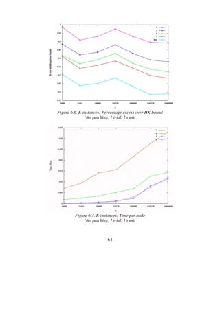
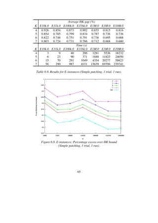
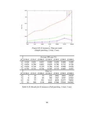
6.1 Performance for E-instances
The E-instances consist of cities uniformly distributed in the 1,000,000 by
1,000,000 square under the Euclidean metric. For testing purposes I have
selected those instances of 8th
DIMACS Implementation Challenge that
have 10,000 or more cites. Optima for these instances are currently un-
known. I follow Johnson and McGeoch [24] in measuring tour quality in
terms of percentage over the Held-Karp lower bound [16, 17] on optimal
tours. The Held-Karp bound appears to provide a consistently good ap-
proximation to the optimal tour length [22].
Table 6.1 covers the lengths of the current best tours for the E-instances.
These tours have all been found by LKH. The first two columns give the
names of the instances and their number of nodes. The column labeled CBT
contains the lengths of the current best tours. The column labeled HK bound
contains the Held-Karp lower bounds. The table entries for the two largest
instances (E3M.0 and E10M.0), however, contain approximations to the
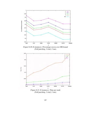
Held-Karp lower bounds (lower bounds on the lower bounds).](https://image.slidesharecdn.com/koptreport-150110102502-conversion-gate01/85/Koptreport-52-320.jpg)
![53
The column labeled HK gap (%) gives for each instance the percentage ex-
cess of the current best tour over the Held-Karp bound:
HK gap (%) =
CBT HK bound
HK bound
100%
It is well known that for random Euclidean instances with n cities distrib-
uted uniformly randomly over a rectangular area of A units, the ratio of the
optimal tour length to n A approaches a limiting constant COPT as n .
Johnson, McGeoch, and Rothenberg [21] have estimated COPT to 0.7124 ±
0.0002. The last column of Table 6.1 contains these ratios. The results are
consistent with this estimate for large n.
Instance n CBT HK bound
HK gap
(%)
CBT
n
10 6
E10k.0 10,000 71,865,826 71,362,276 0.706 0.7187
E10k.1 10,000 72,031,896 71,565,485 0.652 0.7203
E10k.2 10,000 71,824,045 71,351,795 0.662 0.7182
E31k.0 31,623 127,282,687 126,474,847 0.639 0.7158
E31k.1 31,623 127,453,582 126,647,285 0.637 0.7167
E100k.0 100,000 225,790,930 224,330,692 0.651 0.7140
E100k.1 100,000 225,662,408 224,241,789 0.634 0.7136
E316k.0 316,228 401,310,377 398,582,616 0.684 0.7136
E1M.0 1,000,000 713,192,435 708,703,513 0.633 0.7132
E3M.0 3,162,278 1,267,372,053 1,260,000,000 0.585 0.7127
E10M.0 10,000,000 2,253,177,392 2,240,000,000 0.588 0.7125
Table 6.1. Tour quality for E-instances.
Using cutting-plane methods Concorde [1] has found a lower bound of
713,003,014 for the 1,000,000-city instance E1M.0 [4]. The bound shows
that LKH’s tour for this instance has a length at most 0.027% greater than
the length of an optimal tour.](https://image.slidesharecdn.com/koptreport-150110102502-conversion-gate01/85/Koptreport-53-320.jpg)

![55
Figure 6.2. 5 -nearest candidate set for E10k.0.
For each value K between 2 and 8 ten local optima were found, each time
starting from a new initial tour. Initial tours are constructed using self-
avoiding random walks on the candidate edges [18].
The results from these experiments are shown in Table 6.2. The table covers
the Held-Karp gap in percent and the CPU time in seconds used for each
run. The program parameter PATCHING_C specifies the maximum number
of cycles that may be patched during the search for moves. In this experi-
ment, the value is zero, indicating that only non-sequential moves are to be
considered. Note, however, that the post optimization procedure of LKH for
finding improving non-sequential 4- or 5-opt moves is used in this as well
as all the following experiments.](https://image.slidesharecdn.com/koptreport-150110102502-conversion-gate01/85/Koptreport-55-320.jpg)

![68
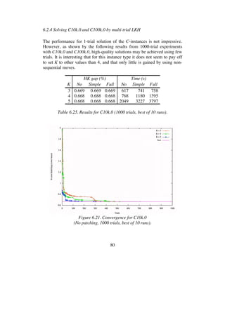
6.1.4 Solving E10k.0 and E100k.0 by multi-trial LKH
In the experiments described until now only one trial per run was used. As
each run takes a new initial tour as its starting point, the trials have been in-
dependent. Repeatedly starting from new tours, however, is an inefficient
way to sample locally optimal tours. Valuable information is thrown away.
A better strategy is to kick a locally optimal tour (that is, to perturb it
slightly), and reapply the algorithm on this tour. If this effort produces a
better tour, we discard the old tour and work with the new one. Otherwise,
we kick the old tour again. To kick the tour the double-bridge move (see
Figure 2.4) is often used [2, 3, 29].
An alternative strategy is used by LKH. The strategy differs from the stan-
dard approach in that it uses a random initial tour and restricts its search
process by the following rule:
Moves in which the first edge (t1,t2) to be broken belongs to
the current best solution tour are not investigated.
It has been observed that this dependence of the trials almost always results
in significantly better tours than would be obtained by the same number of
independent trials. In addition, the search restriction above makes it fast.
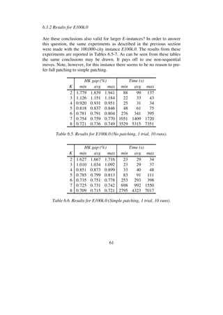
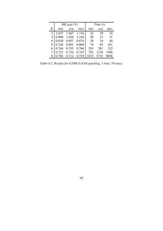
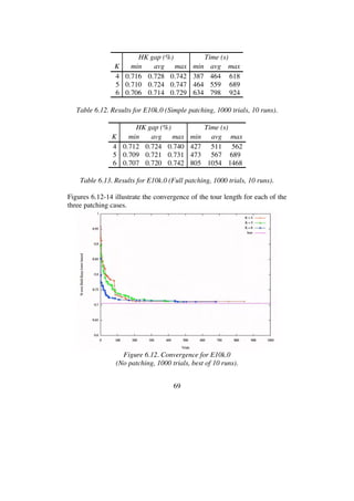
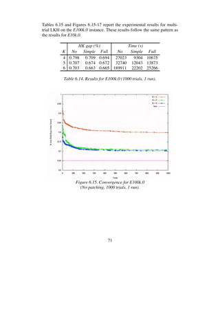
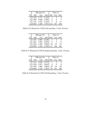
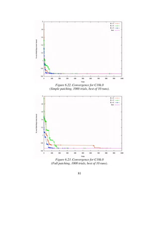
I made a series of experiments with the instances E10k.0 and E100k.0 to
study how multi-trial LKH is affected when K is increased and cycle patch-
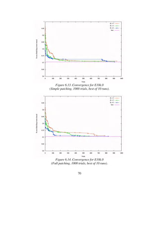
ing is added to the basic K-opt move. Tables 6.11-13 report the results for
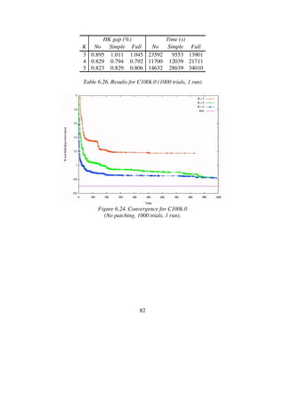
1000 trials on E10k.0. As can be seen, tour quality increases as K increases,
and as in the previous 1-trial experiments with this instance it is advanta-
geous to use cycle patching (simple patching seems to be a better choice
than full patching).
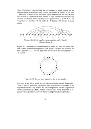
HK gap (%) Time (s)
K min avg max min avg max
4 0.712 0.728 0.741 512 569 640
5 0.711 0.720 0.745 444 564 750
6 0.711 0.716 0.724 1876 2578 4145
Table 6.11. Results for E10k.0 (No patching, 1000 trials, 10 runs).](https://image.slidesharecdn.com/koptreport-150110102502-conversion-gate01/85/Koptreport-68-320.jpg)
![73
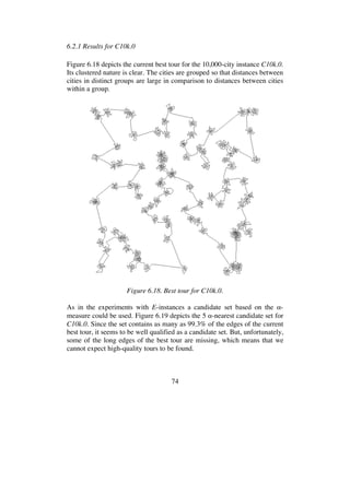
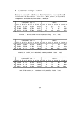
6.2 Performance for C-instances
It is well known that geometric instances with clustered points are difficult
for the Lin-Kernighan heuristic. When it tries to remove an edge bridging
two clusters, it is tricked into long and often fruitless searches. Each time a
long edge is removed, the cumulative gain rises enormously, and the heu-
ristic is encouraged to perform very deep searches. The cumulative gain
criterion is too optimistic and does not effectively prune the search space for
this type of instances [32].
To examine LKH’s performance for clustered problems I performed ex-
periments on the eight largest C-instances of the 8th
DIMACS TSP Chal-
lenge. Table 6.15 covers the lengths of the current best tours for these in-
stances. These tours have all been found by LKH. My experiments with C-
instances are very similar to those performed with the E-instances.
Table 6.15. Tour quality for C-instances.
Instance n CBT HK bound HK gap (%)
C10k.0 10,000 33,001,034 32,782,155 0.668
C10k.1 10,000 33,186,248 32,958,946 0.690
C10k.2 10,000 33,155,424 32,926,889 0.694
C31k.0 31,623 59,545,428 59,169,193 0.636
C31k.1 31,623 59,293,266 58,840,096 0.770
C100k.0 100,000 104,646,656 103,916,254 0.703
C100k.1 100,000 105,452,240 104,663,040 0.754
C316k.0 316,228 186,936,768 185,576,667 0.733](https://image.slidesharecdn.com/koptreport-150110102502-conversion-gate01/85/Koptreport-73-320.jpg)
![75
Figure 6.19. 5 -nearest candidate set for C10k.0.
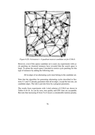
For geometric instances, Johnson [20] has suggested using quadrant-based
neighbors, that is, the least costly edges in each of the four geometric
quadrants (for 2-dimensional instances) around the city. For example, for
each city its neighbors could be chosen so as to include, if possible, the 5
closest cities in each of its four surrounding quadrants.
For clustered instances I have chosen to use candidate sets defined by the
union of the 4 -nearest neighbors and the 4 quadrant-nearest neighbors (the
closest city in each of the four quadrants). Figure 6.20 depicts this candidate
set for C10k.0. Even though this candidate subgraph is very sparse (average
number of neighbors is 5.1) it has proven to be sufficiently rich to produce
excellent tours. It contains 98.3% of the edges of the current best tour,
which is less than for the candidate subgraph defined by 5 -nearest neigh-
bors. In spite of this, it leads to better tours.](https://image.slidesharecdn.com/koptreport-150110102502-conversion-gate01/85/Koptreport-75-320.jpg)
![84
6.3 Performance for M-instances
The testbed of the 8th
DIMACS TSP Challenge also contains seven in-
stances specified by distance matrices where each entry is chosen independ-
ently and uniformly from the integers in (0,1000000]. Sizes range from
1,000 to 10,000. All have been solved to optimality.
This type of instances appears to be easy to LKH-2. I have chosen only to
report the results of my experiments with the largest of these instances, the
10,000-city instance M10k.0.
6.3.1 Results for M10k.0
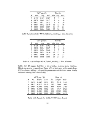
Tables 6.27-29 report the results of the 1-trial runs. As optimum is known
for this instance, I will measure tour quality as the percentage excess over
optimum. The tables show that high-quality solutions can be obtained using
only one trial, and with running times that are small, even for K = 8.
OPT gap (%) Time (s)
K min avg max min avg max
3 0.167 0.200 0.238 1 1 1
4 0.038 0.053 0.077 1 1 1
5 0.013 0.022 0.031 1 1 1
6 0.006 0.012 0.016 2 3 3
7 0.003 0.007 0.010 4 4 5
8 0.001 0.005 0.009 6 8 10
Table 6.27. Results for M10k.0 (No patching, 1 trial, 10 runs).](https://image.slidesharecdn.com/koptreport-150110102502-conversion-gate01/85/Koptreport-84-320.jpg)
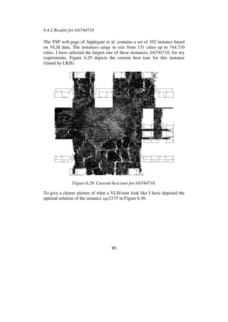
![86
6.4 Performance for R-instances
The preceding sections have presented computational results from experi-
ments with synthetic generated test instances. In order to study the perform-
ance of LKH-2 for real world instances I made experiments with three
large-scale instances from the TSP web page of Applegate, Bixby, Chvátal
and Cook [39]. These instances are listed in Table 6.31. The column labeled
CBT contains the length of the current best tour for each of the instances.
Instance n CBT
ch71009 71,009 4,566,506
lrb744710 744,710 1,611,420
World 1,904,711 7,515,964,553
Table 6.31. R-instances.
Optima for these instances are unknown. The current best tours have been
found by LKH. Since the Held-Karp lower bounds are not available, I will
measure tour quality as percentage excess over these tours (CBT gap).](https://image.slidesharecdn.com/koptreport-150110102502-conversion-gate01/85/Koptreport-86-320.jpg)
![87
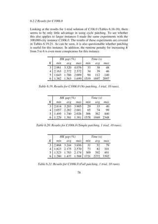
6.4.1 Results for ch71009
The TSP web page of Applegate et al. contains a set of 27 test instances de-
rived from maps of real countries, ranging in size from 28 cities in Western
Sahara to 71,009 cities in China. I have selected the largest one of these in-
stances, ch71009, for my experiments. Figure 6.27 depicts the current best
tour for this instance (found by LKH).
Figure 6.27. Current best tour for ch71009.
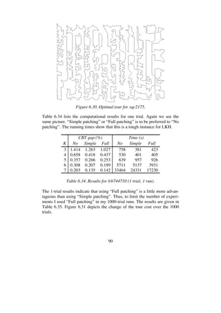
The Concorde package [1] was used to compute a lower bound for ch71009
of 4,565,452. This bound shows that LKH’s best tour is at most 0.024%
greater than the length of an optimal tour.
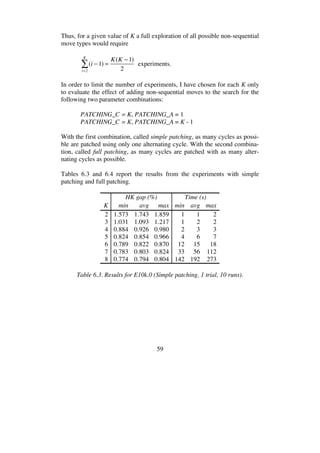
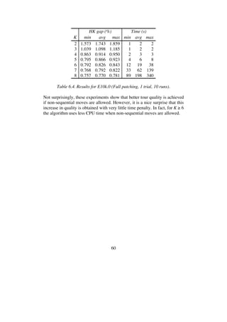
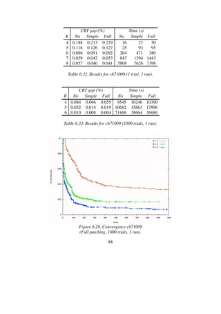
Table 6.32 lists the computational results for one trial. The results indicate
that “Simple patching” or “Full patching” is to be preferred to “No patch-
ing”. In this respect ch71009 resembles E-instances. The advantage of using
patching is further emphasized by the 1000-trial results shown in Table
6.33. Note that the 1000-trial run with K = 6 and full patching results in a
tour that deviates only 0.004% from the current best tour.](https://image.slidesharecdn.com/koptreport-150110102502-conversion-gate01/85/Koptreport-87-320.jpg)
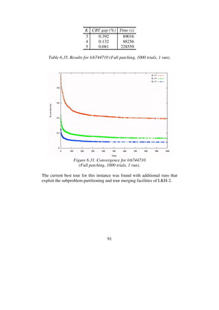
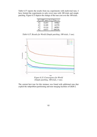
![92
6.4.3 Results for World
The largest test instance on the TSP web page of Applegate et al. is a
1,904,711-city instance of locations throughout the world, named World.
Figure 6.32 depicts the current best tour for this instance (found by LKH).
Figure 6.32. Projection of current best tour for World.
The Concorde package [1] was used to compute a lower bound of
7,512,276,947 for this instance (August 2007). This bound shows that LKH-
2’s best tour has length at most 0.049% greater than the length of an optimal
tour.
As can be seen from Figure 6.32, this instance is clustered. So in my ex-
periments I used the same candidate neighborhood as was used for the C-
instances, i.e., the 4 -nearest neighbors supplemented with the 4 quadrant-
nearest neighbors. In addition, the so-called Quick-Boruvka algorithm [3]
was used to construct the initial tour. I found that this tour construction al-
gorithm improved the tour quality considerably in my 1-trial runs. Table
6.36 lists the computational results from these runs.
CBT gap (%) Time (s)
K No Simple Full No Simple Full
3 1.072 0.915 1.011 4911 867 974
4 0.658 0.567 0.505 2881 1508 1459
5 0.490 0.301 0.316 3802 3736 7485
6 0.275 0.235 0.228 20906 15788 61583
Table 6.36. Results for World (1 trial, 1 run).](https://image.slidesharecdn.com/koptreport-150110102502-conversion-gate01/85/Koptreport-92-320.jpg)

![95
References
[1] D. Applegate, R. Bixby, V. Chvátal, and W. Cook,
“Concorde: A code for solving Traveling Salesman Problems” (1999),
http://www.tsp.gatech.edu/concorde.html
[2] D. Applegate, R. Bixby, V. Chvátal, and W. Cook,
“Finding tours in the TSP”,
Technical Report 99885, Forschungsinstitut für Diskrete Mathematik,
Universität Bonn (1999).
[3] D. Applegate, W. Cook, and A. Rohe,
“Chained Lin-Kernighan for Large Traveling Salesman Problems”,
Technical Report 99887, Forschungsinstitut für Diskrete Mathematik,
Universität Bonn (2000).
[4] D. Applegate, R. Bixby, V. Chvátal, and W. Cook,
“Implementing the Dantzig-Fulkerson-Johnson Algorithm for Large
Traveling Salesman Problems”,
Mathematical Programming, 97, pp. 91-153 (2003).
[5] V. Bafna and P. Pevzner,
“Genome rearrangements and sorting by reversals”,
SIAM Journal on Computing, 25(2), pp. 272-289 (1996).
[6] A. Bergeron,
“A Very Elementary Presentation of the Hannenhalli-Pevzner Theory”,
Lecture Notes in Computer Science, 2089, pp. 106-117 (2001).
[7] A. Caprara,
“Sorting by reversals is difficult”,
In Proceedings of the First International Conference on Computational
Molecular Biology, pp. 75-83 (1997).
[8] B. Chandra, H. Karloff and C. Tovey,
“New results on the old k-opt algorithm for the TSP”,
In Proceedings of the 5th Annual ACM-SIAM Symposium on Discrete
Algorithms,
pp. 150-159 (1994).](https://image.slidesharecdn.com/koptreport-150110102502-conversion-gate01/85/Koptreport-95-320.jpg)
![96
[9] N. Christofides and S. Eilon,
“Algorithms for large-scale traveling salesman problems”,
Operations Research Quarterly, 23, pp. 511-518 (1972).
[10] M. L. Fredman, D. S. Johnson, L. A. McGeoch, and G. Ostheimer,
“Data Structures for Traveling Salesmen”,
J. Algorithms, 18(3) pp. 432-479 (1995).
[11] B. Funke, T. Grünert and S. Irnich,
“Local Search for Vehicle Routing and Scheduling Problems: Review and
Conceptual Integration”.
Journal of Heuristics, 11, pp. 267-306 (2005).
[12] D. Garg and A. Lal,
”CS360 - Independent Study Report”,
IIT-Delhi (2002).
[13] G. Gutin and A. P. Punnen,
“Traveling Salesman Problem and Its Variations”,
Kluwer Academic Publishers (2002).
[14] P. J. Hanlon, R. P. Stanley, and J. R. Stembridge,
“Some combinatorial aspects of the spectra of normally distributed random
matrices”.
Contemporary Mathematics, 138, pp. 151-174 (1992).
[15] S. Hannenhalli and P. A. Pevzer,
“Transforming cabbage into turnip: polynomial algorithm for sorting signed
permutations by reversals”,
In Proceedings of the 27th ACM-SIAM Symposium on Theory of
Computing, pp. 178-189 (1995).
[16] M. Held and R. M. Karp,
“The traveling-salesman problem and minimum spanning trees”,
Operations Research, 18, pp. 1138-1162 (1970).
[17] M. Held and R. M. Karp,
“The traveling-salesman problem and minimum spanning trees: Part II”,
Math. Programming, pp. 6-25 (1971).](https://image.slidesharecdn.com/koptreport-150110102502-conversion-gate01/85/Koptreport-96-320.jpg)
![97
[18] K. Helsgaun,
“An Effective Implementation of the Lin-Kernighan Traveling Salesman
Heuristic”,
European Journal of Operational Research, 12, pp. 106-130 (2000).
[19] H. H. Hoos and T. Stützle,
“Stochastic Local Search: Foundations and Applications”,
Morgan Kaufmann (2004).
[20] D. S. Johnson,
“Local optimization and the traveling salesman problem”,
Lecture Notes in Computer Science, 442, pp. 446-461 (1990).
[21] D. S. Johnson, L. A. McGeoch, and E. E. Rothberg,
“Asymptotic Experimental Analysis for the Held-Karp Traveling Salesman
Bound”,
Proc. 7th Ann. ACM-SIAM Symp. on Discrete Algorithms, pp. 341-350
(1996).
[22] D. S. Johnson and L. A. McGeoch,
“The Traveling Salesman Problem: A Case Study in Local Optimization”
in Local Search in Combinatorial Optimization, E. H. L. Aarts and J. K.
Lenstra (editors), John-Wiley and Sons, Ltd., pp. 215-310 (1997).
[23] D. S. Johnson, L. A. McGeoch, F. Glover, and C. Rego,
“8th
DIMACS Implementation Challenge: The Traveling Salesman Problem”
(2000),
http://www.research.att.com/~dsj/chtsp/
[24] D. S. Johnson and L. A. McGeoch,
“Experimental Analysis of Heuristics for the STSP”,
In The Traveling Salesman Problem and Its Variations, G. Gutin and A.
Punnen, Editors, pp. 369-443 (2002).
[25] H. Kaplan, R. Shamir, and R. E. Tarjan,
“Faster and simpler algorithm for sorting signed permutations by reversals”,
In Proc. 8th annual ACM-SIAM Symp. on Discrete Algorithms (SODA 97),
pp. 344-351, 1997.](https://image.slidesharecdn.com/koptreport-150110102502-conversion-gate01/85/Koptreport-97-320.jpg)
![98
[26] E. L. Lawler, J. K. Lenstra, A. H. G. Rinnooy Kan, and D. B. Shmoys
(eds.),
“The Traveling Salesman Problem: A Guided Tour of Combinatorial
Optimization”,
Wiley, New York (1985).
[27] S. Lin and B. W. Kernighan,
“An Effective Heuristic Algorithm for the Traveling-Salesman Problem”,
Operations Research, 21, pp. 498-516 (1973).
[28] K. T. Mak and A. J. Morton,
“Distances between traveling salesman tours”,
Discrete Applied Mathematics, 58, pp. 281-291 (1995).
[29] O. Martin, S.W. Otto, and E.W. Felten,
“Large-step markov chains for the tsp incorporating local search heuristics”,
Operations Research Letters, 11, pp. 219-224 (1992).
[30] D. Mendivil, R.Shonkwiler, and M. C. Spruill,
“An analysis of Random Restart and Iterated Improvement for Global
Optimization with an application to the Traveling Salesman Problem”,
Journal of optimization theory and applications, 124 (4), pp. 407-433
(2005).
[31] A. Möbius, B. Freisleben, P. Merz, and M. Schreiber,
“Combinatorial Optimization by Iterative Partial Transcription”,
Physical Review E, 59 (4), pp. 4667-4674 (1999).
[32] D. Neto.
“Efficient Cluster Compensation For Lin-Kernighan Heuristics”,
PhD thesis, University of Toronto (1999).
[33] M. Okada,
“Studies on Probabilistic Analysis of –opt for Traveling Salesperson
Problems”,
Doctor’s thesis, Nara Institute of Science and Technology (1999).
[34] L. K. Platzman and J. J. Bartholdi,
“Spacefilling curves and the planar traveling salesman problem”,
Journal of the ACM, 36(4), pp. 719-737 (1989).](https://image.slidesharecdn.com/koptreport-150110102502-conversion-gate01/85/Koptreport-98-320.jpg)
![99
[35] A. Rohe,
“Parallele Heuristiken fur sehr gro e Traveling Salesman Probleme”,
Diplomarbeit, Research Institute for Discrete Mathematics, Universität
Bonn (1997).
[36] A. Rohe,
“Parallel Lower and Upper Bounds for Large TSPs”,
ZAMM, 77(2), pp. 429-432 (1997).
[37] E. Tannier, M. Sagot,
“Sorting by reversals in subquadratic time”,
Rapport de recherche No
5097, l’INRIA (2004).
[38] W. Zhang and M. Looks,
“A Novel Local Search Algorithm for the Traveling Salesman Problem that
Exploits Backbones”,
IJCAI 2005, pp. 343-350 (2005).
[39] “Traveling salesman problem web”,
http://www.tsp.gatech.edu/
[40] “The On-Line Encyclopedia of Integer Sequences”,
http://www.research.att.com/~njas/sequences/A061714](https://image.slidesharecdn.com/koptreport-150110102502-conversion-gate01/85/Koptreport-99-320.jpg)

This document summarizes an implementation of k-opt moves for the Lin-Kernighan traveling salesman problem heuristic. It describes LKH-2, which allows k-changes for any k from 2 to n. This generalizes a previous version, LKH-1, which uses 5-changes. The effectiveness of LKH-2 is demonstrated on instances with 10,000 to 10 million cities, finding high-quality solutions in polynomial time like the original Lin-Kernighan heuristic.