SlideShare a Scribd company logo
1 of 111
Journal of Health Economics 4 (1985) 63-78. North-Holland
RELATIVE INCQMES AND RATES OF RETURN
FOR U.S. PHYSICIANS*
Philip L. BURSTEIN and Jerry CROMWELL
Centerfor Health Economics Research, Chestnut Hill, M.4
022167, USA
Received March 1983, final version received August 1984
Since 1967 the supply of physicians in the U.S. hgs been
growing by more than 3 percent per
annum. This, coupled with public insurer fee discounts, might
have been expected to depress
both the relative and absolute incomes of physicians in spite of
growing insurance coverage and
new technologies. Real incomes of physicians did decline at a
0.2 percent annual rate between
1967 and 1980, but this was apparently due to c;conomy-wide
events since the income trends for
lawyers, dentists, and college graduates were virtually identical.
Internal rates of return to
undergraduate medical training remained high - between 14 and
17 percent in 1980. Specialty
training became more profitable for internists, general surgeons,
and obstetricians/gynecologists
(all with 10-15 percent rates of return), while pediatricians
continued to suffer a financial loss.
While Medicare and Medicaid fee discounts have been criticized
as inequitable, the programs
are also shown to provide a ‘hidden subsidy’ to physicians
during residency training, materially
adding to rates of returns.
1. Introduction
In this paper we examine trends in the real incomes of United
States
physicians over time. We wish to determine whether any of the
three
pecuniary incentives for individuals to become physicians -
high absolute
incomes, high incomes relative to other professional groups,
and high rates of
return to medical training - have become less powerful. There
are two
reasons for supposing that this might have occurred. The first is
the very
rapid increase in the supply of physicians that has occurred in
recent years.
Over 1967-80 the ratio of active ph,u. l+ians to population rose
3.3 percent
annually, with the number of internists and pediatricians going
up at a
particularly rapid rate. During the pre-Medicare/Medicaid
period (1951~67),
physicians per capita grew only 0.2 percent per year, so recent
developments
in physician supply represent a marked departure from earlier
experience.
The second possible reason for a slower growth in incomes of
physicians is
the reduction, over time, in the proportion of the usual
physician fee paid by
the two major public insurance programs (Medicare and
Medicaid). By the
end of our study period Medicare discounted the usual fee for a
follow-up
*Supported under HCFA Grant no. 18-P-97723/1-01, Alice
Litwinowicz, Project Gfftcer.
0167-6296/85/$3.30 0 1985, Elsevier Science Publishers B.V.
(North-Holland)
64 P.L. But-stein and J. Cromwell, U.S. physician4 incomes
office visit by 16 percent, while the Medicaid discount was 34
percent
[Mitchell et al. (1981)]. This payment policy may have been to
offset the
large increase in demand brought about by these programs,
which was
putting severe pressure on government budgets. Whether these
discounts
were more or less than the bad debts physicians had been
incurring on the
poor and elderly prior to 1966 is uncertain, but that they greatly
expanded
overall demand (and income) is undebatable.
While a considerable literature’ on the rate of return to medical
education
does exist, it is not suitable for time-series analysis due to
incomparable (and
limited) analysis years, varying comparison groups, and
incompatible
methodologies. The present work, which presents a consistent
time series for
rates of return to both undergraduate and specialized medical
training,
ena.bles the hypothesis of declining income status for
physicians to be
systematically investigated over a much longer time period than
heretofore.
Moreover, data were collected to enable us to make adjustments
for such
frequently neglected factors as schooling subsidies and resident
salaries,
among other things.
The remainder of this paper is in five parts. In section 2, data
on the
incomes of physicians and three comparison groups - lawyers,
dentists and
college graduates - are presented for the 1951-80 period. In
section 3, our
methodology for estimating the rates of return to medical
education, both
undergraduate and specialized, is discussed, including key
adjustments. In
section 4, internal rates of return for medical, dental, and legal
education are
calculated. In section 5, rates of return to specialty training are
presented for
four types of primary care physicians: internists, general
surgeons,
obstetricians/gynecologists, and pediatricians. The last section
provides a
brief discussion of the policy implications. Our overall
conclusion is that the
financial incentives for entering the medical profession suffered
very little
diminution over the study period, in spite of the rapid growth in
the
physicians per capita ratio and public insurer discounts. There
is no evidence
that this situation will change significantly in the near future.
2. Pncomes of physicians and ot II prsfessionals
2.1. Data sources
The primary data needed for the rate of return calculations
concern the
income and hours worked of physicians, lawyers, dentists and
college
‘See, for example, Eangwell(1982), Dresch (1981), Mennemeyer
(1978), Sloan (1970), Feldman
and Schemer (1976). AMA (1973) and Lindsay (1973). These
papers and other, earlier efforts on
this topic were .summarized in the longer report from which the
present work is drawn. See
Cromwell and Burstein (1982, ch. 5).
P.L. Burstein and J. Cromwell, U.S. physicians’ incomes 65
graduates.2 The basic sources of income data are given in table
1, but a few
notes are required. The AMA survey data (as reported in the
annual Profile
of Medical Practice) overlap the Goldstein (1972) physician
income series in
1969; it was assumed that the same proportional difTerence
would have
existed in earlier years and the Goldstein figures were adjusted
accordingly.
The pre-1968 figures on the mean income of physicians by
specialty were
obtained by taking median income data from Medical
Economics and
converting them to means by use of the assumption that the
mean/median
income ratio was the same for all specialists in any given year.
Table 1’
Physician and other professional average net incomes,b 1951-
80,
current dollars.
Period Physicians Lawyers
1980 %85,600 $35,819
1979 78,400 32,771
1978 65,508 30,093
1977 61,200 27,583
1976 59,500 26,170
1975 56,408 24,665
1974 5~ooo 22,923
1973 48,600 21,666
1972 47,200 20,382
1971 45,300 19,210
1970 41,800 18,296
1969 39,727 17,083
1967 35,729 15,276
1965 29,589 14,233
1963 - 13,223
1961 23,659 12249
1959 22,239 -
1955 17,215 -
1951 13,432 -
Dentists
-
-
$48,363
-
42,035
-
35,698
3&O
-
30,770
24,740
20,698
-
16,020
14,849
12,480
10,388
College
graduates’
$28,306
26,300
24,529
22,585
20,896
19,684
18,011
17,518
16,972
15,565
14,675
14,670
11,973
-
-
-
-
-
-
%ources: Physicians - 1969-80: American Medical Associ-
ation, Projle of Medical Practice; 1955-67: Goldstein (1972,
table
16); 1951: Survey of Current Business. Lawyers - U.S. Bureau
of
Labor Statistics, National Survey of Professional,
Administrative,
Technical, and CZericaZ Pay [Bulletins 2/45 (1982) and 2004
(1978)]. Dentists - Journal of the American Dental Association.
College graduates - U.S. Bureau of the Census, Current Popul-
ation Reuorts. Series P-60: Current Income, Education, and
ARe.
bGross’ revenue less professional
income tax.
expenses before -payment of
CMales over 25, working full time.
2The class of ‘college graduates’ includes only those with no
post-college schooling.
66 P.L. Burstein and .I. Cromwell, U.S. physicians’ incomes
Because the AMA figures are based on self-reports, the
accuracy of the
income figures is open to question. While independent surveys
(e.g., HCFA’s
annual physician survey) give very similar figures once sample
differences are
accounted for, underreporting of deferred income may still be a
serious
problem. To the extent this problem pervades all the reported
incomes of
professionals, no bias in internal rates of return comparisons
obtains
although absolute income trends may be understated. Given the
very high
rates of return shown below, the amount of underreporting is
probably not
too serious.
Data on annual hours of work (post-1968 only) for physicians,
lawyers and
dentists were taken from the same sources as the income ,data.
Comparison
figures for college graduates were obtained by use of the
formula reported by
Kniesner (1976),
HOURS = 2574.3 - 1 1 1.2(real hourly wage) + 27.3(years of
education)
+ 194(wife’s wage) - 7.7(age) -t- 6.9(years at current job)
- 203.9 (race).
In applying this formula, the hourly wage was taken from the
previous year
(assumed unchanged 1978-79), a non-working spouse was
assumed, and the
other variables were set to appropriate values for the average
college
graduate of the year in question. (Race represented the
proportion of non-
white graduates.)
Fcr the adjustments to the basic rate of return figures, a variety
of sources
were used. Data on medical school tuition came from the annual
reports on
medical education found in the Journal of the American Medical
Association,
while the data on medical school grants came from this source
and from
Feldman (1980). Goldstein (1972) supplied data on stipends for
interns and
residents Over the 1965-69 period, Feldman (1980) for 1977,
and Hough
(1981) for 1974-79. A constant rate of annual real growth over
1970-74 was
assumed.
2.2. Income trertds
Table 1 shows that the annual nominal net incomes of
physicians rose
from $13,432 to $85,600 over the period 1951-80, an increase
of 539 percent.
Even after allowing for inflation, the total real increase was
101.4 percent, or
2.4 percent per year. In the last year for which comparable data
exist,
physicians did very well in comparison with lawyers, dentists
and male
college graduates. In fact, physicians’ mean earnings were more
tha. double
P.L. Burstein and J. Cromwell, U.S. physicians’ incomes 67
those of lawyers, and triple those of male college graduates,
while exceeding
those of dentists by more than one-third. This superiority of
physician
incomes over relevant comparison groups holds for every year
for which data
exist.
An interesting question is whether any trend unfavorable to
physicians
developed at some point during the study period. Table 2
contains the
information necessary to investigate this possibility. In the
1952-67 pre-
Medicare/Medicaid period, the tea! rate of growth of
physicians’ incomes was
4.7 percent per year. The post-program rate of growth, however,
was actually
negative, at -0.2 percent per year. Thus, as high as the growth in
nominal
physician incomes was, it failed to keep pace with inflation.
Table 2
Growth rates in real professional incomes, selected sub-periods.
Period Physicians Lawyers Dentists
College
graduates
Total
1951-80 2.3% - 2.4%” -
Pre- and post-
proRram
1951-67 4.7 - 3.9
1967-80 -0.2 -0.3 0.0” -;1
Sub-periods
1972-80 -0.8 - 1.2 - 1.5” - 1.4
1967-72 1.1 1.3 1.8 2.5
1961-67 5.2 1.9 5.6 -
1951-61 4.2 - 2.9 -
‘Last data year is 1978.
Can this reversal in the extremely favorable earnings trend of
the pre-
program period be ascribed to changes in supply/demand
conditions specific
to the market for medical services? This is doubtful for two
reasons:
-Physician incomes continued to rise through 1972, with the
decline in real
earnings for the entire post-program period due to post-1973
trends, and
-All other professional and educational comparison groups for
which we
have data show similar income trends over time, in spite of
being
completely unaffected by Medicare and Medicaid.
Both of these patterns are clear in table 2 and fig. 1. In the
latter, the solid
vertical line which indicates the start of Medicare and Medicaid
is not
associated with any break in the earlier rising income trend.
Over the first
68 P.L. Burstein and .I. Cromwell, U.S. physicians’ incomes
1980 $
90,000
80,000
70,000
60,OOC
50,00(
40,001
30,oo
d
1
Y L
1 53 55 57 59 61 63 65 67 69 71 73 75 77 79 80
Fig. 1. Real professional incomes, 1951430.
P.L. Burstein and J. Cromwell, U.S. physicians’ incomes 69
part of the post-program period (1967-76), average physician
income
increased 1.1 percent per year. The second part of the post-
program period
(1972~80), on the other hand, saw on 0.8 percent per year real
income
decline. All three of our comparison groups - lawyers, dentists
and male
college graduates - also had real income declines between 1972
and 1980.
(The income of high school graduates showed a similar pattern,
with a 2.1
percent annual rate of increase followed by a -0.8 percent rate
of decline.)
The all-inclusive nature of the fall in real income indicates that
some
economy-wide phenomenon - probably the high and accelerating
rate of
inflation - was responsible for much, if not all, of the post-
program decline
in real physician incomes.
The rehtive income situation is also interesting. Physician
earnings were
virtually constant between 1967-80 relative to the three
comparison groups.
The result vis-Lvis dentists is surprising, since the growth in
dental insurance
coverage was extremely rapid during this period3 while the
supply of dentists
was growing relatively more slowly (0.6 percent annual increase
over the
1967-80 period versus 3.3 percent for physicians). It is quite
possible that
other, offsetting factors like the spread of fluoridation negated
dentistry’s
positive insurance effects, producing demand trends comparable
with those of
physicians experiencing slower insurance growth but more
demand-inducing
technical change, e.g., endoscopies, radionucleide and CAT
scanning. There is
nothing overt in the net income data that shows any impact of
physician
supply increases or deeper public insurance fee discounts on
average
physician incomes. This is a serious matter if it means that
private financial
incentives will not retard the current trend toward physician
oversupply.
Alternatively, if insurance and technology trends simply
overwhelmed
burgeoning supply effects in the 197Os, then the direct and
indirect demand
controls so prevalent in the 1980s (e.g., higher deductibles and
copays) could
have a material effect on future supplies.
It has been demonstrated above that physicians are maintaining
their
relative and absolute income superiority over a sample of other
professionals.
Another and perhaps more important influence on the decision
of potential
new practitioners to enter the medical profession is the rate of
financial
return. This aspect 0; long-run physician supply is considered
below.
3. Methodology for calculating rates of return
As noted above, it is extremely difficult to draw any
conclusions
concerning rates of return to medical training from the existing
literature.
Years of analysis are limited in the individual studies, and no
two estimates
‘The percentag e o f the U.S. population with private dental
insurance rose from 3-23 percent
1967-77.
70 P.L. Burstein and J. Cromwell, U.S. physicians’ incomes
are comparable. The present paper is unique in that a uniform
approach is
used to evaluate. rates of return, over a substantial period of
time.
3.1. The basic formula
Our basic rate of return
Suppose that we wish to
formula is taken from Sloan and Feldman (1978).
compute the rate of return for group 2, which
differs from the base group 1 primarily in that the former has
undertaken an
additional period of training. The present value Vi of the annual
income Y1
earned by group 1 (assuming that the income flow continues
forever) is
(1)
where S1 is the first year of the income flow and tl is the
appropriate
discount rate for this group. Integrating this formula gives
V, =(Y1/rl)e-‘IS1. (2)
If group 2 spends more time in training than group 1, we can
find the
internal rate of return r to that investment by tinding the
discount rate which
equates V, to V,. This gives us
(Y~/r)e-rSI=(Y,/r)e-‘S2, (3)
which implies that
YJY, =e’%-%). (4)
Since, by definition, annual earnings Y equals the hourly wage
W times the
number of hours worked per year L for each
pecuniary benefits are equal, our unadjusted
becomes
group, and assuming non-
internal rate of return );
Eq. (5) is, of course, based on differences in annual earnings. If
we assume
that any gap between L, and L2 is induced by differences in the
hou.rly wage
and not any non-pecuniary benefits, then an equally valid
formula would be
ra=ln(KIK)/(S,-U, (6)
where r, is interpreted as the hours-adjusted internal rate of
return. If leisure
has some value, and certain assumptions (see below) are
satisfied, then the
P.L. Burstein and J. Cromwell, U.S. physicians’ inc0me.s 71
true internal rate of return r to the additional training obtained
by group 2
will lie somewhere between this hours-adjusted rate ra and r,.
To demonstrate this, it is useful to make the additional
assumption that
the supply curve of labor is the same for the two groups and not
perfectly
inelastic. This implies that by voluntary choice, L2 >I,, in all
relevant
situations, ceteris paribus .4 For this extra labor time, group 2
will receive
IV.,& -I,,) in additional earnings. However, not all of this
earnings
increment can be considered to be a true return. To obtain the
extra money,
group 2 individuals must give up (L, -IL,) hours of leisure. The
net return to
the extra work effort of group 2 is equal to the monetary return
minus the
value of the foregone leisure. Therefore, rates of return based
on annual
earnings unadjusted for differences in hours (e.g., P,) will
overstate the actual
benefit of belonging to group 2. Rates of return based on hourly
earnings
alone (e.g., r,J will understate the true rate of return, however,
since some
positive benefit must accrue to group 2 for the extra hours
worked, for
otherwise they would not have worked longer. Thus, if our basic
formulas
are correct, we may conclude that r,c~cr,.
3.2. Adjustments
The rate of return formulas (5) and (6) are based on a number of
implicit
assumptions which would tend to cause inaccuracies when
applied to the
earnings of physicians. These assumptions include:
-A constant length of physician training,
-An equal (and infinite) work life for all groups,
- Zero out-of-pocket educational costs for post-college training,
-Zero earnings for medical residents,
- Similar earnings/experience profiles for all groups.
We made corrections for the first four of these, using the
methods described
below. We were unable to deal with the last item, so our rate of
return
estimates will be slight overestimates since the lifetime
earnings advantage of
physicians is concentrated somewhat in their later years.
3.2.1. Finite working lifetimes
The first adjustment made to the basic formulas deals with the
fact that
workers do retire at a finite age. This means that the present
value formula
(1) represen ts an overestimate of actual discounted earnings.
The error will
be greater for those professions with the shortest working lives
(or longest
training). Our response was to reduce the & employed in the
rate of return
formulas by a factor of Vi/q, where v is retirement-adjusted
present value
4We are assuming that the extra training has some monetary
value.
72 P.L. Burstein and J. Cromwell, U.S. physicians* incomes
of lifetime earnings, truncated at a fixed retirement age of 65 in
(1). A
discount rate of 10 percent was assumed. Perhaps contrary to a
priori
expectations, Vi/y varied from only 0.967 (physicians 1978) to
0.986 (college
graduates). Potential earnings past age 65 are simply not of
much
importance to decisions made at age 21, due to the operation of
the discount
rate.5 This adjustment thus reduced the calculated rate of return
to medical
education by a maximum of 0.3 percentage points - an
insignificant change
as we shall see.
This result is quite sensitive to the time discount rate employed.
At a 5
percent rate, assuming a fixed, age 65 retirement rate for all
occupations
reduces the return to medical education by 2.3 percentage
points. Unlike
many college graduates, however, physicians enjoy a longer,
more lucrative
career which is ignored in using a 65 age limit. According to the
latest AMA
figures [AMA (1984)], 16.2 percent of GPs were still in active
practice over
age 65, working 45 hours per week, and enjoying a net income
of $64,300
(compared to $116,500 for those in the peak earnings years, 46-
55). Without
knowing exactly the true rate of time discount and recognizing
the unequal
retirement ages of college graduates and physicians, ail we can
say is that the
true adjustment probably lies somewhere between 0.3 and 2.3
percentage
points.
3.2.2. Rising medical school costs
Even with this adjustment, our rate of return formula does not
take into
account the out-of-pocket costs for more years of formal
schooling. It is well
known that medical school tuition rose sharply during the
197Os, from an
average of $1,379 in 1970 to $5,287 in 1980 [Hadley (1980),
JAMA (1983)].
Less well known, however, is the extraordinary rise in grants to
medical
students that took place over 1968-71 [Feldman (1980)], which
caused a
sharp decline in net annual tuition per medical student from
approximately
$2,200 to $1,700 per year (real 1967 dollars). The 1967 peak in
real net
tuition, in fact, was not surpassed until 1977, as the increase in
grants almost
exactly matched the rise in tuition over the 1971-75 period. To
calculate the
impact of these offsetting changes, the sum of the average net
tuition over the
four years of medical school was divided by the present value of
total
earnings for physicians to get a proportional reduction in the
income figure
to be used ‘in the rate of return formula. It was determined that
net lifetime
income was reduced approximately 2 percent when cost of
education was
taken into accotmt, resulting in a decline in the rate of return of
close to 0.5
percentage points.
?his same point applies to the longer-thaz;avsrage working lives
of physicians; the extra
earnings from additional time in the labor force occur too far in
the future to have any impact.
A full year of extra earnings at age 66, for example, is
discounted by a factor of 74 (from the
viewpoint of a 21 year old with a 10 percent discount rate).
P.L. Burstein and J. Cromwell, U.S. physicians’ incomes 73
3.63. Rising earnings of medical residents
Finally, the substantial growth in earnings of physicians during
their
residency period ($15,000 per year, median, by 1979) were
taken into account
in similar fashion. The large increase in these earnings coupled
with their
timing early in a physician’s career made this an important
factor. Calculated
lifetime discounted earnings increased by between 2.6 to 8.8
percent under
this adjustment at its peak (k977), with the specialties requiring
longer
training obviously benefiting the most from higher residency
salaries. The
average rate of return for all physicians relative to college
students increased
by 0.8 percentage points, while the rate of return for general
surgeons (with
the longest training/residency period) relative to general
practitioners
increased by 1.5 percentage points in 1977.
3.2.4. Net impact of adjustments
The approximate net impacts of the three adjustments
considered here
were a 0.8 percentage point decrease in the calculated rate of
return to a basic
medical education, and a maximum 0.7 percentage point
increase in the rate of
return to specialized medical training. Both of these rates were
lowered by the
adjustments for finite working life (-0.3) and out-of-pocket
costs of in-class ~
training (-0.5), while the adjustment for the earnings of
residents (+ 1.5)
applied to the rate of return for specialists only.
4. Rates of return to physicians’ post-college training
To compute the rate of return to post-college training, the
incomes of
physicians, dentists and lawyers were compared to those of
college graduates.
This is appropriate for dentists and lawyers since the decision to
enter a
professional school takes effect at the end of college, and no
further decisions
concerning investment in formal education must be made. For
physicians,
however, the choice of specialty made at the end of professional
school
vitally affects their future income and rate of return, as we shall
show.
Therefore, to calculate the rate of return to the first post-college
training
decision, i.e., to become a ‘doctor’, the impact of physician
specialization
must be deleted. This is achieved by computing rates of return
for the group
of physicians that did not undertake specialty training - the
general
practitioners. While the rate of return to all physician training
was also
calculated, it is the rate of return for general practitioners which
is most
comparable to the figures given for dentists and lawyers.
Our results are given in table 3. They indicate that physicians,
dentists and
lawyers all earned a positive return on their post-college
training. The
adjusted rate of return for general practitioners was between
12.1 and 14.5
percent, and the unadjusted rate ranged from 16.3 to 19.0
percent. In
P.L. Burstein and J. Cromwell, U.S. physicians’ incomes
Table 3
Internal rates of return,” 1967-80.
Year All physicians
r. r”
General
practitioners
r. rU
Dentists Lawyersb
r. rU rU
1980
1979
1978
1977
1976
1975
1974
1973
1972
1971
1970
1967
12.1% 14.0% 14.2%
11.6 13.7 14.5
11.0 13.2 13.0
10.2 12.6 13.3
10.5 13.3 12.4
11.6 14.2 12.3
12.0 14.3 14.5
10.8 13.8 12.5
10.7 14.2 12.2
11.6 15.1 13.2
11.8 14.7 12.1
11.3 14.3 12.5
11.7 15.5 13.2
16.7%
17.2
16.3
17.0
16.4
16.7
18.2
17.4
17.8
18.9
16.8
17.2
19.0
- - 7.2%
16.3% - 14.9% 7.2 6.8
- - 6.8
15.8 14.9 7.1
- - 7.1
14.9 14.8 7.1
- - 6.7
14.4 14.8 5.7
- - 6.6
16.1 15.7 7.0
- - 4.7
13.5 15.4 7.7
4; is the hours adjusted rate of return, and r, is the unadjusted
rate.
bNo ra was calculated for lawyers due to lack of data on hours
of work for this
group.
.
absolute terms, this was surely more than adequate to attract
new entrants
into the profession of medicine. In relative terms, the general
practitioner’s
rate was far superior to that of lawyers, and approximately
equal to that of
dentists. There is no indication of any major trend in the rate of
return to
initial post-college training for any of the professions. This is
contrary to
what we would expect if medical supply/demand factors had
reduced
physician incomes.
The lower figure for the all-physician rate of return deserves
some
discussion. This pattern is almost certainly due to the movement
toward
increased specialization in the medical profession. If the
marginal rate of
return to medical education declines with additional years of
training (which
is in accordance with both investment theory and the figures
presented in the
next section), then increasing specialization must bring down
the average rate
of return for all physicians. It should be noted, however, that
this average
rate of return will have no impact on either the medical school
or the
specialization decision, which are affected only by the marginal
return rates.
Also note the difference between unadjusted and adjusted rates.
The latter
are lower, reflecting the longer average work weeks of
physicians. On average
the basic return to medical school is reduced about 4 points, or
roughly 25
percent. This differential appears to be narrowing markedly
over time,
implying relative declines in physician work effort compared to
other
professionals. While consistent with the increase in the supply
of physicians,
P.L. Burstein and .?. Cromwell, U.S. physicians’ incomes 75
reduced work effort per physician makes the ability of the
medical profession
to keep their incomes up to previous standards even more
difficult to explain
unless major changes in practice organization and technology
have improved
their overall productivity.
5. Rates of return to some important specialties
The groups chosen for study in this section are the general
surgeons,
obstetricians/gynecologists, internists and pediatricians. For
calculating the
rates of return to these specialists, general practitioners
constitute our
reference group. This is appropriate because the decision to
enter a medical
specialty can be taken only at the end of undergraduate medical
training.
Based on board-certification requirements, we assumed that
general surgeons
needed five years of post-medical school training,
obstetricians/gynecologists
four, and internists and pediatricians three.(j The results are
given in table 4.
Except for the pediatricians, specialization seems to have been
highly profitable
in the most recent years listed. Averaging the 1977-80 figures,
internists
Year
Table 4
Internal rates of return to specialty training.”
General Obstetricians-
Internists surgeons gynecologists
r, TU r, r, r, r,
Pediatricians
rU r,
1980
1979
1978
1977
1976
1975
1974
1973
1972
1971
1970
1969
1967
1955
1951
9.8% 11.3
11.4 11.2
8.9 6.3
10.3 13.3 E
12.5 ii:3
8.0 6.1
7.5 6.3
4.9 4.2
4.6 4.3
9.3 10.8
4.7 7.1
8.3 12.0
- n.a.
- n.a.
13.6 11.3
12.5 10.6
11.9 10.6
10.8 9.4
12.5 11.5
11.6 il.2
9.1 8.1
9.2 10.2
8.8 9.1
8.8 9.1
11.2 11.2
9.7 9.1
7.4 6.8
6.2 n.a.
3.7 n.a.
14.8 14.0
14.2 11.4
9.5 8.4
11.5 10.0
13.0 10.3
12.1 10.5
11.7 9.7
10.2 9.2
9.3 7.6
9.1 6.3
11.8 10.0
8.4 7.3
7.5 8.0
10.0 n.a.
4.9 n.a.
- -
ii 3.0 - 2.3
- -
- 2.0
2.4 ii
- -
1.6 -
0.6 n.a.
4.1 n.a.
9, is the hours adjusted rate of return, and r, is the unadjusted
rate. ‘-’ indicates a
negative rate of return.
“These figures were obtained from Wechsler (1976, table 1).
Feldman (19gO) asserts that four
years is a better estimate for a ‘typical’ internist, but he agrees
with the other figures. The one
year graduate medical education requirement for licensure has
been ignored for GPs.
76 P.L. Burstein and J. Cromwell, U.S. physicians’ incomes
received a rate of return of 10.6-11.3 percent, general surgeons
11.0-13.1
percent, and obstetricians 12.7-14.5 percent, while pediatricians
suffered an
income loss. 7 Going back to the years immediately following
the
introduction of Medicare and Medicaid (1967-69), we observe
uniformly
lower rates; internists received a rate of return between 9.6 and
6.5 percent,
general surgeons 6.5-8.6 percent, obstetricians 7.7-8.0 percent,
and
pediatricians a negative return. Thus, except for pediatrics, the
financial
incentive to enter a specialty held up well in the post-program
period. In
fact, the rate of return to internists, general surgeons and
obstetricians rose
by 3.9, 4.5, and 5.8 percentage points, respectively, during this
time. These
increases represent a substantial fraction of the original return
rates.
It is interesting to note that the increased rates of return for the’
three
profitable specialties cited here were not matched by an
equivalent increase
in the returns to general practitioners. Between 1967-69 and
1979-80 the GP
rate of return rose by only 0.3 percentage points. Continuation
of this trend
for another decade would remove the general
practitioner/specialty return
rate differential completely. The movement toward increasing
specialization
has thus received added impetus from the private financial
considerations of
medical students. Pediatrics is obviously the exception; any
individual
entering this specialty must be strongly influenced by non-
monetary
considerations.
6. Conclusion
The conventional picture of medicine as a financially attractive
profession
is strongly confirmed by this study. The difference in absolute
incomes
between physicians, on the one hand, and dentists and lawyers
on the other
was 35 and 139 percent, respectively, in 1978-80; this
advantage will
unquestionably remain large in the forseeable future.
The internal rate of return to basic medical training exceeded 12
percent in
every post-Medicare/Medicaid year, ‘ii:i;ng apprtiximatcly
equal to that for
dental education and roughly double the rate for law school.
Medical
specialization in the areas of internai medicine, general surgery
and
obstetrics/gynecology was also highly profitable, with the rates
of return
increasing substantially since the late 1960s. Pediatrics was the
sole exception
to this general picture of financial success, with decliuing birth
rates and
limited insurance perhaps being responsible for the negative
rate of return to
training in this specialty. (Their patients are ineligible for
Medicare, and
other insurers generally do not cover routine child care.)
‘The first number given for each speckity is the average af the
1977 and 1980 adjusted rates
of return, and the second is the average of the unadjusted rates
for the same years. It is not
possible to exactly quantify any negative rate of return using
the methods of this paper.
P.L. Burstein and .l. Cromwell, U.S. physicians’ incomes 77
It is perhaps somewhat surprising that rates of return to medical
training
managed to stay so high in the face of (a) increasing fee
discounts for public
insurers, (b) rapidly growing physician supply, and (c) rising
tuition costs.
The first of these may be more apparent than real if physicians
manipulate
the ‘usual’ fees on which these discounts are calculated.
Cromwell and
Burstein (1982), for example, have shown that physicians only
rarely receive
full payment of their usual charge while Lee and Hadley (1981)
demonstrate
the po:;litive relationship between ‘usuals’ and usual-
customary-reasonable
payment m&hods as part of a revenue-maximizing game.
Second, burgeoning
supply could have been offset by increasing intensity per visit,
which also is
well documented for recent years (Cromwell et al. (1982),
Freeland and
Schendler (198l)J The third was shown to be counteracted by
rising
financial support for medical students, so that no significant
increase in net
medical school tuitio,1 was recorded over the 1967-80 period.
The increase in
the stipends of medical residents was a fourth factor, which was
working to
increase rates of return for specialty training substantially.
One policy conclusion to emerge from the analysis is that
programs
designed to reduce total medical expenditures by limiting
physician incomes
can be enacted without serious impact on the financial
attractiveness of this
profession. Rates of return to medicine are not only high on an
absolute
basis, but equal or exceed those of other forms of post-graduate
training.
While non-pecuniary factors could explain the systematically
higher returns
(e.g., a distaste for the ‘sight of blood’, the long, arduous
schooling),
institutional rigidities probably explain the larger part of the
differential. The
ability of the profession to influence medical school admissions
and licensure
exams, as well as their resistance to legal delegation of more
routine tasks to
other health professionals, has certainly helped perpetuate their
economic
advantage [Sloan (1970), Frech (1974), Kessel(l970)].
Another conclusion points to the ‘hidden subsidy’ afforded
physicians by
all insurers, including Medicare and Medicaid. Increased
insurance coverage
has enhanced returns not only by raising the demand of the
elderly and the
poor, but by increasing the remuneration of residents via cost-
based
reimbursement of teaching hospitals. Since only specialists in
training receive
the benefits of this change, this could be one of the important
factors behind
the enhanced rates of return for specialty training. Given the
enormous
financial advantage to a medical education, insurers might
reconsider their
policy of including resident salaries as a fully allowable
expense.
References
American Medical Association, 1973, Measuring physician
manpower: Contritiutiorss to a
comprehensive health manpower strategy (Center for Health
Services Research and Develop-
ment, Chicago, IL).
American Medical Association, 1984, The American health care
system.
78 P.L. Burstein and J. Cromwell, U.S. physicians’ incomes
Cromwell, Jerry and Philip L. Burstein, 1982, Physician losses
from Medicare/Medicaid
participation: How real are they? (Center for Health Economics
Research, Chestnut Hill,
MA).
Cromwell, Jerry, J. Mitchell and P. Burstein, 1982, Analysis of
changes in the content of
physician office visits: Descriptive analysis of NAMCS, Report
to DHHS/HRA, contract no.
232-81-0039.
Dresch, Stephen P., 1981, Marginal wage rates, hours of work
and returns to physician
specialization, in: Nancy Greenspan, ed., Issues in physician
reimbursement: Health care
linancing conference proceedings, DHHS publication no.
(HCFA) 03121 (Department of
Health and Human Services, Washington, DC) 165-200.
Feldman, Roger D., 1980, Loan programs and medical education
financing in: Jack Hadley, ed.,
Medical education financing (Neale Watson, New York) 94-127.
Feldman, Roger D. and R.M. Scheffler, 1976, The supply of
medical school applicants and the
rate of return to training (Economics Department, University of
North Carolina, Chapel
Hill, NC).
Frech, H.E., 1974, Occupational licensure and health care
productivity: The issues and the
literature, in: J. Rafferty, ed., Health manpower and
productivity (Heath, Lexington, MA)
119-142.
Freeland, Mark S. and C. Schendler, 1981, National health
expenditures: Short-term outlook
and long-term projections, Health Care Financing Review 2,97-
138.
Goldstein, Marcus S., 1972, Income of physicians, osteopaths
and dentists from professional
practice, 196569, DHEW publication no. (SSA) 73-11852
(Department of Health Education
and Welfare, Washington, DC).
Hadley, Jack, 1980, Introduction, in: Jack Hadley, ed., Medical
education financing (Neale
Watson, New York) l-22.
Hough, Douglas, 1981, The economic status of resident
physicians, in: David Goldfarb, ed.,
Profile of medical practice (American Medical Association,
Monroe, WI) 83-96.
Journal of the American Medical Association, 1983,83rd Annual
report on me&al education in
the U.S.
Kessel, Reuben A., 1970, The AMA and the supply of
physicians, Law and contemporary
problems, Health Care 35, no. 2, Part I, 267-283.
Kniesner, T.J., 1976, An indirect test of complementarity in the
family labor supply model,
Econometrica 34,651-670.
Langwell, Kathryn M., 1982, Sex differences in returns to
physicians’ choice of specialty, Journal
of Health Politics, Policy and Law 7, 752-761.
Lee, Robert and J. Hadley, 1981, Physicians’ fees and public
medical care programs, Health
Services Research 16, 185-203.
Lindsay, Cotton M., 1973, Real returns to medical education,
Journal of Human Resources 8,
331-348.
Mennemeyer, Stephen T., 1978, Really great returns to medical
education, Journal of Human
Resources 13,75-90.
Mitchell. Janet B. et al., 1981, Physician participation in public
programs (Center for Health
Economics Research, Chestnut Hill, MA).
Sloan, Frank A., 1970, Lifetime earnings and physicians’ choice
of specialty, Industrial and
Labor Relations Review 24, 49.
Sloan, Frank A. and Roger Feldman, 1978, Competition among
physicians, in: Warren
Greenberg, ed., Competition in the health care sector: Past,
present, and future, Proceedings
of a conference sponsored by the Bureau of Economics, FTC,
57-131.
Wechsler, Henry, 1976, Handbook of medical specialties
(Human Services Press, New York).
On the Concept of Health Capital
and the Demand for Health
Michael Grossman
National Bureau of Economic Research
The aim of this study is to construct a model of the demand for
the
commodity ''good health." The central proposition of the model
is that
health can be viewed as a durable capital stock that produces an
output
of healthy time. It is assumed that individuals inherit an initial
stock
of health that depreciates with age and can be increased by
investment.
In this framework, the "shadow price" of health depends on
many other
variables besides the price of medical care. It is shown that the
shadow
price rises with age if the rate of depreciation on the stock of
health
rises over the life cycle and falls with education if more
educated people
are more efficient producers of health. Of particular importance
is the
conclusion that, under certain conditions, an increase in the
shadow
price may simultaneously reduce the quantity of health
demanded and
increase the quantity of medical care demanded.
I. Introduction
During the past two decades, the notion that individuals invest
in them-
selves has become widely accepted in economics. At a
conceptual level,
increases in a person's stock of knowledge or human capital are
assumed
to raise his productivity in the market sector of the economy,
where he
produces money earnings, and in the nonmarket or household
sector,
where he produces commodities that enter his utility function.
To realize
This paper is hased on part of my Columbia University Ph.D.
dissertation, "The
Demand for Health: A Theoretical and Empirical Investigation,"
which will be pub-
lished by the National Bureau of Economic Research. My
research at the Bureau was
supported by the Commonwealth Fund and the National Center
for Health Services
Research and Development (PHS research grant 2 P 01 HS
00451-04). Most of this
paper was written while I was at the University of Chicago's
Center for Health Ad-
ministration Studies, with research support from the National
Center for Health Ser-
vices Research and Development (PHS grant HS 00080). A
preliminary version of this
paper was presented at the Second World Congress of the
Econometric Society. I am
grateful to Gary S. Becker, V. K. Chetty, Victor R. Fuchs,
Gilbert R. Ghez, Robert T.
Michael, and Jacob Mincer for their helpful comments on earlier
drafts.
2 2 4 JOURNAL OF POLITICAL ECONOMY
potential gains in productivity^ individuals have an incentive to
invest
in formal schooling or in on-the-job training. The costs of these
invest-
ments include direct outlays on market goods and the
opportunity cost
of the time that must be withdrawn from competing uses. This
frame-
work has been used by Becker (1967) and by Ben-Porath (1967)
to
develop models that determine the optimal quantity of
investment in
human capital at any age. In addition, these models show how
the
optimal quantity varies over the life cycle of an individual and
among
individuals of the same age.
Although several writers have suggested that health can be
viewed as
one form of human capital (Mushkin 1962, pp. 129-49; Becker
1964,
pp. 33-36; Fuchs 1966, pp. 90-91), no one has constructed a
model of the
demand for health capital itself. If increases in the stock of
health simply
increased wage rates, such a task would not be necessary, for
one could
simply apply Becker's and Ben-Porath's models to study the
decision to
invest in health. This paper argues, however, that health capital
differs
from other forms of human capital. In particular, it argues that a
person's
stock of knowledge affects his market and nonmarket
productivity, while
his stock of health determines the total amount of time he can
spend
producing money earnings and commodities. The fundamental
difference
between the two types of capital is the basic justification for the
model
of the demand for health that is presented in the paper.
A second justification for the model is that most students of
medical
economics have long realized that what consumers demand
when they
purchase medical services are not these services per se but,
rather, '̂ good
health." Given that the basic demand is for good health, it
seems logical
to study the demand for medical care by first constructing a
model of
the demand for health itself. Since, however, traditional demand
theory
assumes that goods and services purchased in the market enter
consumers'
utihty functions, economists have emphasized the demand for
medical
care at the expense of the demand for health. Fortunately, a new
approach
to consumer behavior draws a sharp distinction between
fundamental ob-
jects of choice—called ^'commodities'^-—and market goods
(Becker 1965;
Lancaster 1966; Muth 1966; Michael 1969; Becker and Michael
1970;
Ghez 1970). Thus, it serves as the point of departure for my
health
model. In this approach, consumers produce commodities with
inputs of
market goods and their own time. For example, they use
traveling time
and transportation services to produce visits; part of their
Sundays and
church services to produce ''peace of mind"; and their own time,
books,
and teachers' services to produce additions to knowledge. Since
goods and
services are inputs into the production of commodities, the
demand for
these goods and services is a derived demand.
Within the new framework for examining consumer behavior, it
is
assumed that individuals inherit an initial stock of health that
depreciates
CONCEPT OF HEALTH CAPITAL 225
over time—at an increasing rate, at least after some stage in the
life
cycle—and can be increased by investment. Death occurs when
the stock
falls below a certain level, and one of the novel features of the
model
is that individuals **choose" their length of life. Gross
investments in
health capital are produced by household production functions
whose
direct inputs include the own time of the consumer and market
goods
such as medical care, diet, exercise, recreation, and housing.
The produc-
tion function also depends on certain '^environmental
variables," the
most important of which is the level of education of the
producer, that
influence the efficiency of the production process.
It should be realized that in this model the level of health of an
indi-
vidual is not exogenous but depends, at least in part, on the
resources
allocated to its production. Health is demanded by consumers
for two
reasons. As a consumption commodity, it directly enters their
preference
functions, or, put differently, sick days are a source of
disutility. As an
investment commodity, it determines the total amount of time
available
for market and nonmarket activities. In other words, an increase
in the
stock of health reduces the time lost from these activities, and
the mone-
tary value of this reduction is an index of the return to an
investment
in health.
Since the most fundamental law in economics is the law of the
down-
ward-sloping demand curve, the quantity of health demanded
should be
negatively correlated with its shadow price. The analysis in this
paper
stresses that the shadow price of health depends on many other
variables
besides the price of medical care. Shifts in these variables alter
the
optimal amount of health and also alter the derived demand for
gross
investment, measured, say, by medical expenditures. It is shown
that the
shadow price rises with age if the rate of depreciation on the
stock of
health rises over the life cycle and falls with education if more
educated
people are more efficient producers of health. Of particular
importance is
the conclusion that, under cwtain conditions, an increase in the
shadow
price may simultaneously reduce the quantity of health
demanded and
increase the quantity of medical care demanded.
n . A Stock Approach to the Demand for Health
A, The Model
Let the intertemporal utility function of a typical consumer be
U = U(<f>ono, . . . , <f>nHn, ZQJ , . . , Zn), ( 1 )
where Ho is the inherited stock of health. Hi is the stock of
health in the
iih time period, <t>i is the service flow per unit stock, hi =
</>ifl"̂ is total
consumption of "health services," and Z^ is total consumption
of another
2 2 6 JOURNAL OF POLITICAL ECONOMY
commodity in the ith period.^ Note that, whereas in the usual
inter-
temporal utility function «, the length of life as of the planning
date, is
fixed, here it is an endogenous variable. In particular, death
takes place
when Hi = Hmin- Therefore, length of life depends on the
quantities of
Hi that maximize utility subject to certain production and
resource con-
straints that are now outlined.
By definition, net investment in the stock of health equals gross
invest-
ment minus depreciation:
Hi^^~Hi^h-h,H,, (2)
where Ii is gross investment and 8̂ is the rate of depreciation
during the
fth period. The rates of depreciation are assumed to be
exogenous, but
they may vary with the age of the individual.^ Consumers
produce gross
investments in health and the other commodities in the utility
function
according to a set of household production functions:
(3)
In these equations, Mi is medical care, Xi is the goods input in
the pro-
duction of the commodity Z ,̂ THi and Ti are time inputs, and Ei
is the
stock of human capital.^ It is assumed that a shift in human
capital
changes the efficiency of the production process in the
nonmarket sector
of the economy, just as a shift in technology changes the
efficiency of the
production process in the market sector. The implications of
this treat-
ment of human capital are explored in Section IV.
It is also assumed that all production functions are
homogeneous of
degree 1 in the goods and time inputs. Therefore, the gross
investment
production function can be written as
(4)
where ti ^= THi/Mi. It follows that the marginal products of
time and
medical care in the production of gross investment in health are
1 The commodity Z,- may be viewed as an aggregate of all
commodities besides health
that enter the utility function in period i. For the convenience of
the reader, a glossary
of symbols may be found in Appendix B.
2 In a more complicated version of the model, the rate of
depreciation might be a
negative function of the stock of health. The analysis is
considerably simplified by
treating this rate as exogenous, and the conclusions reached
would tend to hold even
if it were endogenous.
3 In general, medical care is not the only market good in the
gross investment func-
tion, for inputs such as housing, diet, recreation, cigarette
smoking, and alcohol con-
sumption influence one*s level of health. Since these inputs
also produce other
commodities in the utility function, joint production occurs in
the household. For an
analysis of this phenomenon, see Grossman (1970, chap. 6). To
emphasize the key
aspects of my health model, I treat medical care as the most
important market good
in the gross investment function in the present paper.
CONCEPT OF HEALTH CAPITAL 2 2 7
(5)
From the point of view of the individual, both market goods and
own
time are scarce resources. The goods budget constraint equates
the present
value of outlays on goods to the present value of earnings
income over
the life cycle plus initial assets (discounted property income):^
W,TW,
= 2. ^ + ^0- (6)
Here Pi and Vi are the prices of Mi and Xi^ W^ is the wage
rate, TWi is
hours of workj ^o is discounted property income, and r is the
interest rate.
The time constraint requires that Q, the total amount of time
available
in any period, must be exhausted by all possible uses:
TW, + TL, + TH, + T,= Q, (7)
where TLi is time lost from market and nonmarket activities due
to illness
or injury.
Equation (7) modifies the time budget constraint in Becker's
time
model (Becker 1965). If sick time were not added to market and
non-
market time, total time would not be exhausted by all possible
uses. My
model assumes that TL, is inversely related to the stock of
health; that is,
'dTLi/'^Hi < 0. If Q were measured in days (Q = 365 days if the
year
is the relevant period) and if <f>i were defined as the flow of
healthy days
per unit of Hi, h-, would equal the total number of healthy days
in a
given year.^ Then one could write
TL, = Q-h. (8)
It is important to draw a sharp distinction between sick time and
the
time input in the gross investment function. As an illustration of
this
difference, the time a consumer allocates to visiting his doctor
for periodic
checkups is obviously not sick time. More formally, if the rate
of de-
preciation were held constant, an increase in TH.i would
increase U and
Hij^i and would reduce TL^^i. Thus, TH, and TZ^+i would be
negatively
correlated.®
^ The sums throughout this study are taken from f r= 0 to n.
5 If the stock of health yielded other services besides healthy
days, 0̂ would be a
vector of service flows. This study emphasizes the service flow
of healthy days because
this flow can be measured empirically.
6 For a discussion of conditions that would produce a positive
correlation between
and TL^_^_^, see Section III.
2 2 8 JOURNAL OF POLITICAL ECONOMY
By substituting for TWi from equation (7) into equation ( 6 ) ,
one
obtains the single '*full wealth'' constraint:
+ V,X, + W,{TL, + TH, +
(9)
According to equation ( 9 ) , full wealth equals initial assets
plus the present
value of the earnings an individual would obtain if he spent all
of his time
at work. Part of this wealth is spent on market goods, part of it
is spent
on nonmarket production time, and part of it is lost due to
illness. The
equilibrium quantities of Hi and Zi can now be found by
maximizing the
utility function given by equation (1) subject to the constraints
given by
equations ( 2 ) , ( 3 ) , and (9).'' Since the inherited stock of
health and the
rates of depreciation are given, the optimal quantities of gross
investment
determine the optimal quantities of health capital.
B. Equilibrium Conditions
First-order optimality conditions for gross investment in period
i — 1
Uhn
+ . .. + (1 - 8,) ... (1 - K_y) -Y-Gn, (10)
11
The new symbols in these equations are: Vhi ^ "dUfdh; =: the
marginal
utility of healthy days; ^ = the marginal utihty of wealth; Gi-
^'dhi/
i) = the marginal product of the stock of health in
the production of healthy days; and :itt_i = the marginal cost of
gross
investment in health in period i — 1.
"̂ In addition, the constraint is imposed that H^ ^ ^miir
8 Note that an increase in gross investment in period i — 1
increases the stock of
health in all future periods. These increases are equal to
dHi _ _
For a derivation of equation (10), see Part A of the
Mathematical Appendix.
CONCEPT OF HEALTH CAPITAL 2 2 9
Equation (10) simply states that the present value of the
marginal
cost of gross investment in period i — 1 must equal the present
value of
marginal benefits. Discounted marginal benefits at age / equal
I J
where Gi is the marginal product of health capital—the increase
in the
number of healthy days caused by a one-unit increase in the
stock of
health. Two monetary magnitudes are necessary to convert this
marginal
product into value terms, because consumers desire health for
two reasons.
The discounted wage rate measures the monetary value of a one-
unit in-
crease in the total amount of time available for market and
nonmarket
activities, and the term Uh.i/X measures the discounted
monetary equiva-
lent of the increase in utihty due to a one-unit increase in
healthy time.
Thus, the sum of these two terms measures the discounted
marginal value
to consumers of the output produced by health capital.
While equation (10) determines the optimal amount of gross
invest-
ment in period i— 1, equation (11) shows the condition for
minimizing
the cost of producing a given quantity of gross investment.
Total cost is
minimized when the increase in gross investment from spending
an
additional dollar on medical care equals the increase in gross
investment
from spending an addidonal dollar on time. Since the gross
investment
production function is homogeneous of degree 1 and since the
prices of
medical care and time are independent of the level of these
inputs, the
average cost of gross investment is constant and equal to the
marginal
cost.
To examine the forces that affect the demand for health and
gross in-
vestment, it is useful to convert equation (10) into a slightly
different
form. If gross investment in period i is positive, then
. _ i+id^i ( i 4 i ) i + 2 i + 2
/ • * l  ^ I 1 ' / . • •  . * t O I ' " *
(l+r)
Ov _i -I ) ( 1 O« 1 ) vV«( r-.
— . (12)
From (10) and ( 1 2 ) ,
( l - l
( l + ; - ) i - i " (14-ry + ~ I ~ " ^
Therefore,
(13)
)
2 3 0 JOURNAL OF POLITICAL ECONOMY
where JCi_i is the percentage rate of change in marginal cost
between
period i— 1 and period i.^ Equation (13) implies that the
undiscounted
value of the marginal product of the optimal stock of health
capital at
any moment in time must equal the supply price of capital,
7ti^i{r —
jCi_i + 6 0 . The latter contains interest, depreciation, and
capital gains
components and may be interpreted as the rental price or user
cost of
health capital.
Condition (13) fully determines the demand for capital goods
that can
be bought and sold in a perfect market. In such a market, if
firms or
households acquire one unit of stock in period i— 1 at price
Jti_i, they
can sell (1 — hi) units at price Tti at the end of period i.
Consequently,
jt£_i(r — Jti_i + 8,) measures the cost of holding one unit of
capital for
one period. The transaction just described allows individuals to
raise their
capital in period / alone by one unit and is clearly feasible for
stocks like
automobiles, houses, refrigerators, and producer durables. It
suggests that
one can define a set of single-period flow equilibria for stocks
that last
for many periods.
In my model, the stock of health capital cannot be sold in the
capital
market, just as the stock of knowledge cannot be sold. This
means that
gross investment must be nonnegative. Although sales of health
capital are
ruled out, provided gross investment is positive, there exists a
used cost of
capital that in equilibrium must equal the value of the marginal
product
of the stock.̂ *̂ An intuitive interpretation of this result is that
exchanges
over time in the stock of health by an indiadual substitute for
exchanges
in the capital market. Suppose a consumer desires to increase
his stock
of health by one unit in period i. Then he must increase gross
investment
in period i — 1 by one unit. If he simultaneously reduces gross
investment
in period i hy (1 — 8̂ ) units, then he has engaged in a
transaction that
raises Hi and Hi alone by one unit. Put differently, he has
essentially
rented one unit of capital from himself for one period. The
magnitude of
the reduction in It is smaller the greater the rate of depreciation,
and its
dollar value is larger the greater the rate of increase in marginal
cost over
time. Thus, the depreciation and capital gains components are as
relevant
to the user cost of health as they are to the user cost of any
other durable.
Of course, the interest component of user cost is easy to
interpret, for if
one desires to increase his stock of health rather than his stock
of some
other asset by one unit in a given period, rjt^_i measures the
interest
payment he
'^Equation (13) assumes S/5t-_j ^ 0 .
10 For similar conclusions with regard to nonsalable physical
capital and with regard
to a nonsalable stock of ^'goodwill" produced by advertising,
see Arrow (1968) and
Nerlove and Arrow (1962).
11 In a continuous time model, the user cost of health capital
can be derived in one
step. If continuous time is employed, the term b^Ki_^ does not
appear in the user cost
formula. The right-hand side of (13) becomes Jt^(r — jt̂ + 6^),
where K, is the in-
CONCEPT OF HEALTH CAPITAL 2 3 1
A slightly different form of equation (13) emerges if both sides
are
divided by the marginal cost of gross investment:
^ i, (13')
Here Yi = {WiGi)/Ki_i is the marginal monetary rate of return
on an
investment in health and
Uh,
is the psychic rate of return. In equilibrium, the total rate of
return on
an investment in health must equal the user cost of health
capital in terms
of the price of gross investment. The latter variable is defined
as the sum
of the real-own rate of interest and the rate of depreciation.
C. The Pure Investment Model
It is clear that the number of sick days and the number of
healthy days
are complements; their sum equals the constant length of the
period.
From equation (8), the marginal utility of sick time is —Uhi,
Thus, by
putting healthy days in the utility function, one implicitly
assumes that
sick days yield disutility. If healthy days did not enter the
utility function
directly, the marginal monetary rate of return on an investment
in health
would equal the cost of health capital, and health would be
solely an in-
vestment commodity.^- In formalizing the model, I have been
reluctant
to treat health as pure investment because many observers
believe the
demand for it has both investment and consumption aspects
(see, for
example, Mushkin 1962, p. 131; Fuchs 1966, p. 86). But to
simplify the
remainder of the theoretical analysis and to contrast health
capital with
other forms of human capital, the consumption aspects of
demand are
ignored from now on.̂ ^
If the marginal utility of healthy days or the marginal disutility
of sick
days were equal to zero, condition (13') for the optimal amount
of health
capital in period i would reduce to
i. ( 1 4 )
stantaneous percentage rate of change of marginal cost at age i.
For a proof, see Part
B of the Mathematical Appendix.
12 To avoid confusion, a note on terminology is in order. If
health were entirely an
investment commodity, it would yield monetary, but not utility,
returns. Regardless of
whether health is investment, consumption, or a mixture of the
two, one can speak of
a gross investment function since the commodity in question is
a durable.
13 Elsewhere, I have used a pure consumption model to
interpret the set of phenom-
ena that are analyzed in Sections III and IV. In the pure
consumption model, the
marginal monetary rate of return on an investment in health is
set equal to zero (see
Grossman 1970, chap. 3).
232 JOURNAL OF POLITICAL ECONOMY
Equation (14) can be derived explicitly by excluding health
from the
utility function and by redefining the full wealth constraint as^^
' = 0̂ + (15)
Maximization of R' with respect to gross investment in periods i
— 1 and
i yields
+
(1 -f
(16)
+ ...+
(1 —
( 1 - 8 0 . . . (1 - K-
(17)
These two equations imply that (14) must hold.
Figure 1 illustrates the determinations of the optimal stock of
health
capital at any age i. The demand curve MEC shows the
relationship
between the stock of health and the rate of return on an
investment or the
marginal efficiency of health capital, yi- The supply curve S
shows the
relationship between the stock of health and the cost of capital,
r — Si_i
- j - 6i. Since the cost of capital is independent of the stock, the
supply
curve is infinitely elastic. Provided the MEC schedule slopes
downward,
F I G . 1
Since the gross investment production function is homogeneous
of the first degree,
CONCEPT OF HEALTH CAPITAL 233
365
FIG. 2
the equilibrium stock is given by Hi^j where the supply and
demand
curves intersect.
In the model, the wage rate and the marginal cost of gross
investment
do not depend on the stock of health. Therefore, the MEC
schedule would
be negatively inclined if and only if G ,̂ the marginal product of
health
capital, were diminishing. Since the output produced by health
capital has
a finite upper limit of 365 healthy days, it seems reasonable to
assume
diminishing marginal productivity. Figure 2 shows a plausible
relation-
ship between the stock of health and the number of healthy
days. This
relationship may be called the "production function of healthy
days." The
slope of the curve in the figure at any point gives the marginal
product
of health capital. The number of healthy days equals zero at the
death
stock ^min, so that Q = TLi ^ 3 6 5 is an alternative definition
of death.
Beyond ^min, healthy time increases at a decreasing rate and
eventually
approaches its upper asymptote of 365 days as the stock
becomes large.
In Sections I I I and IV, equation (14) and figure 1 are used to
trace out
the lifetime path of health capital and gross investment, to
explore the
effects of variations in depreciation rates, and to examine the
impact of
changes in the marginal cost of gross investment. Before I turn
to these
matters, some comments on the general properties of the model
are in
order. It should be realized that equation (14) breaks down
whenever
desired gross investment equals zero. In this situation, the
present value
of the marginal cost of gross investment would exceed the
present value
of marginal benefits for all positive quantities of gross
investment, and
equations (16) and (17) would be replaced by inequalities.^^
The re-
mainder of the discussion rules out zero gross investment by
assumption,
but the conclusions reached would have to be modified if this
were not
the case. One justification for this assumption is that it is
observed em-
pirically that most individuals make positive outlays on medical
care
throughout their life cycles.
h~i = h =15 Formally, ŷ ̂ ^ — Jtf_i +
2 3 4 JOURNAL OF POLITICAL ECONOMY
Some persons have argued that, since gross investment in health
cannot
be nonnegative, equilibrium condition (14) should be derived by
using the
optimal control techniques developed by Pontryagin and others.
Arrow
(1968) employs these techniques to analyze a firm's demand for
non-
salable physical capital. Since, however, gross investment in
health is
rarely equal to zero in the real world, the methods I use—
discrete time
maximization in the text and the calculus of variations in the
Mathe-
matical Appendix—are quite adequate. Some advantages of my
methods
are that they are simple, easy to interpret, and familiar to most
econo-
mists. In addition, they generate essentially the same
equilibrium condition
as the Pontryagin method. Both Arrow and I conclude that, if
desired
gross investment were positive, then the marginal efficiency of
nonsalable
capital would equal the cost of capital. On the other hand, given
zero
gross investment, the cost of capital would exceed its marginal
efficiency.
The monetary returns to an investment in health differ from the
returns
to investments in education, on-the-job training, and other
forms of human
capital, since the latter investments raise wage rates.^^ Of
course, the
amount of health capital might infiuence the wage rate, but it
necessarily
influences the time lost from all activities due to illness or
injury. To
emphasize the novelty of my approach, I assume that health is
not a
determinant of the wage rate. Put differently, a person's stock of
knowl-
edge affects his market and nonmarket productivity, while his
stock of
health determines the total amount of time he can spend
producing
money earnings and commodities. Since both market time and
nonmarket
time are relevant, even individuals who are not in the labor
force have an
incentive to invest in their health. For such individuals, the
marginal
product of health capital would be converted into a dollar
equivalent by
multiplying by the monetary value of the marginal utility of
time.
Since there are constant returns to scale in the production of
gross
investment and since input prices are given, the marginal cost of
gross
investment and its percentage rate of change over the life cycle
are
exogenous variables. In other words, these two variables are
independent
of the rate of investment and the stock of health. This implies
that con-
sumers reach their desired stock of capital immediately. It also
implies
that the stock rather than gross investment is the basic decision
variable
in the model. By this I mean that consumers respond to changes
in the
cost of capital by altering the marginal product of health capital
and not
the marginal cost of gross investment. Therefore, even though
equation
(14) is not independent of equations (16) and (17), it can be
used to
determine the optimal path of health capital and, by implication,
the
optimal path of gross investment.^'''
difference is emphasized by Mushkin (1962, pp. 132-33).
1*̂ This statement is subject to the modification that the
optimal path of capital must
always imply nonnegative gross investment.
CONCEPT OF HEALTH CAPITAL 235
Indeed, the major differences between my health model and the
human
capital models of Becker (1967) and Ben-Porath (1967) are the
assump-
tions made about the behavior of the marginal product of capital
and the
marginal cost of gross investment. Both Becker and Ben-Porath
assume
that any one person owns only a small amount of the total stock
of
human capital in the economy. Therefore, the marginal product
of his
stock is constant. To rule out solutions in which the desired
stock of
capital is either zero or infinite, they postulate that the marginal
cost of
producing gross additions to the stock is positively related to
the rate
of gross investment. Since marginal cost rises, the desired stock
of human
capital is not reached immediately. Moreover, since the
marginal product
of capital is constant, gross investment is the basic decision
variable in
these models.^^ In my model, on the other hand, the marginal
product of
health capital falls because the output produced by this capital
has a
finite upper limit. Consequently, it is not necessary to introduce
the
assumption of rising marginal cost in order to determine the
optimal
stock.
To illustrate how the implications of the health and human
capital
models differ, suppose the rate of depreciation on either the
stock of health
or human capital rises. This upsets the equality between the cost
of
capital and its marginal efficiency. To restore this equality in
the health
model, the marginal product of health capital must rise, which
would
occur only if the stock of capital declines. To restore this
equality in the
human capital model, marginal cost must fall, which is possible
only if
gross investment declines.^^
HL Life Cycle Variations in Depreciation Rates
Equation (14) enables one to study the behavior of the demand
for
health and gross investment over the life cycle. To simplify the
analysis,
it is assumed that the wage rate, the stock of knowledge, the
marginal cost
of gross investment, and the marginal productivity of health
capital are
independent of age. These assumptions are not as restrictive as
they may
seem. To be sure, wage rates and human capital are undoubtedly
cor-
related with age, but the effects of shifts in these variables are
treated in
Section IV. Therefore, the results obtained in this section may
be viewed
as partial effects. That is, they show the impact of a pure
increase in age
on the demand for health, with all other variables held constant.
IS For a complete discussion of these points, see Becker (1967,
pp. 5-12) and Ben-
Porath (1967, pp. 353-61). For models of the demand for
physical capital by firms in
which the marginal cost of investment and the amount of
investment are positively
correlated, see, for example, Eisner and Strotz (1963) and
Gould (1968).
1^ Section I I I demonstrates that an increase in the rate of
depreciation on health
capital might cause gross investment to increase.
236 JOURNAL OF POLITICAL ECONOMY
Since marginal cost does not depend on age, Jti_i — 0 and
equation
(14) reduces to
K (18)
It is apparent from equation (18) that, if the rate of depreciation
were
independent of age, a single quantity of H would satisfy the
equality
between the marginal rate of return and the cost of health
capital. Con-
sequently, there would be no net investment or disinvestment
after the
initial period. One could not, in general, compare ^ 0 and H^
because
accumulation in the initial period would depend on the
discrepency be-
tween the inherited stock and the stock desired in period 1. This
dis-
crepency in turn would be related to variations in H^y and other
variables
across individuals. But, given zero costs of adjusting to the
desired level
immediately, H would be constant after period 1. Under the
stated
condition of a constant depreciation rate, individuals would
choose an
infinite life if they choose to hve beyond period 1. In other
words, if
Hx > ^min? then Hi would always exceed the death stock.-^
To permit the demand for health to vary with age, suppose the
rate of
depreciation depends on age. In general, any time path of hi is
possible.
For example, the rate of depreciation might be negatively
correlated with
age during the early stages of the life cycle. Again, the time
path might be
nonmonotonic, so that hi rises during some periods and falls
during others.
Despite the existence of a wide variety of possible time paths, it
is ex-
tremely plausible to assume that 6̂ is positively correlated with
age after
some point in the life cycle. This correlation can be inferred
because, as
an individual ages, his physical strength and memory capacity
deteriorate.
Surely, a rise in the rate of depreciation on his stock of health is
merely
one manifestation of the biological process of aging. Therefore,
the anal-
ysis focuses on the effects of an increase in the rate of
depreciation with
age.
Since a rise in 8̂ causes the supply curve of health capital to
shift up-
ward, it would reduce the quantity of health capital demanded
over the
life cycle. Graphically, an increase in the cost of capital from r
--hi to
r-|-8.i_|_i in figure 3 reduces the optimal stock from Hi to i^i+i.
The
greater the elasticity of the MEC schedule, the greater the
decrease in
the optimal stock with age. Put differently, the slower the
increase in the
marginal product of health capital as H falls, the greater the
decrease in
the optimal stock.
Differentiation of equation (18) with respect to age quantifies
the
percentage rate of decrease in the stock of health over the life
cycle:
(19)
-0 The possibility that death can occur in period 1 is ruled out
from now on.
CONCEPT OF HEALTH CAPITAL 237
r + 5
F I G . 3
In this equation, the tilde notation denotes a percentage time
derivative
{Hi^= (dHi/di) (I/Hi), etc.), and the new symbols are: 5̂ = 6i/ 8
:= the share of depreciation in the cost of health capital and
d nHi — —d
e.,- = —
the elasticity of the MEC schedule (In stands for natural
logarithm).^^
Equation (19) indicates that the absolute value of the percentage
de-
crease in H is positively related to the elasticity of the MEC
schedule,
the share of depreciation in the cost of health capital, and the
percentage
rate of increase in the rate of depreciation. If ê and 8,- were
constant, the
curve relating In Hi to age would be concave unless r = 0, s i ^
^
(20)
di
The absolute value of Hi increases over the life cycle because
depre-
ciation's share in the cost of capital rises with age.
21 From equation (18), ln(r + 6 )̂ =nW + ]D.G^ — In JT.
Therefore,
8.- 8a
H,
or
-2 Differentiation of (19) with respect to age yields
or
2 3 8 JOURNAL OF POLITICAL ECONOMY
If 8; grows continuously with age after some point in the life
cycle,
persons would choose to live a finite life. Since H declines over
the life
cycle, it would eventually fall to i?min, the death stock. When
the cost of
health capital is r + 8n in figure 3, Hn — Hmin, and death
occurs. At
death, no time is available for market and nonmarket activities,
since
healthy time equals zero. Therefore, the monetary equivalent of
sick time
in period n would completely exhaust potential full earnings,
Wn^- More-
over, consumption of the commodity Zn would equal zero, since
no time
would be available for its production if total time equals sick
time.̂ -̂ Be-
cause individuals could not produce commodities, total utility
would be
driven to zero at death.-^
Having characterized the optimal path of H,, one can proceed to
ex-
amine the behavior of gross investment. Gross investment's life
cycle
profile would not, in general, simply mirror that of health
capital. In
other words, even though health capital falls over the life cycle,
gross
investment might increase, remain constant, or decrease. This
follows
because a rise in the rate of depreciation not only reduces the
amount of
health capital demanded by consumers but also reduces the
amount of
capital supplied to them by a given amount of gross investment.
If the
change in supply exceeded the change in demand, individuals
would have
an incentive to close this gap by increasing gross investment.
On the
other hand, if the change in supply were less than the change in
demand,
gross investment would tend to fall over the life cycle.
To predict the effect of an increase in hi with age on gross
investment,
note that the net investment can be approximated by HiHir''
Since gross
investment equals net investment plus depreciation.
(21)
Differentiation of equation (21) with respect to age yields
+ hiHi + Hu + 8A
rii + Oi
Suppose hi and ê were constant. Then from (19) and ( 2 0 ) ,
the expres-
sion for Ii would simplify to
23 The above s t a t e m e n t assumes t h a t Z- cannot be
produced with X^ alone. This
would be true if, say, the production function were Cobb-
Douglas.
24 Utility equal zero when H = ^nijn provided the death time
utiUty function is
such t h a t U{0) = 0 .
25 T h a t is,
TJ TJ TJ ' U TJ
dt Hi
The use of this approximation essentially allows one to ignore
the one-period lag be-
tween a change in gross investment and a change in the stock of
health.
CONCEPT OF HEALTH CAPITAL 239
7 8(1 — ̂ ê) (hi — f
Since health capital cannot be sold, gross investment cannot be
nega-
tive. Therefore, hi ^ —Hi.̂ ^ That is, if the stock of health falls
over the
life cycle, the absolute value of the percentage rate of net
disinvestment
cannot exceed the rate of depreciation. Provided gross
investment does
not equal zero, the term 8̂ — SiSb in equation (22) must exceed
zero. It
follows that a sufficient condition for gross investment to be
positively
correlated with the depreciation rate is e < l/si. Thus, Ii would
definitely
be positive at every point if 8 < 1.
The important conclusion is reached that, if the elasticity of the
MEC
schedule were less than 1, gross investment and the depreciation
rate
would be positively correlated over the life cycle, while gross
investment
and the stock of health would be negatively correlated. Phrased
differ-
ently, given a relatively inelastic demand curve for health,
individuals
would desire to offset part of the reduction in health capital
caused by
an increase in the rate of depreciation by increasing their gross
invest-
ments. In fact, the relationship between the stock of health and
the num-
ber of healthy days suggests that 8 is smaller than 1. A general
equation
for the healthy-days production function illustrated by figure 2
is
hi = 365-BHr^, (23)
where B and C are positive constants. The corresponding MEC
schedule
~ (C + 1) In i7^ + In Ŵ — In Jt. (24)
The elasticity of this schedule is given by
din Hi 1
e = = < 1,
a i n y . ( 1 + C ) ^
since C > 0.
Observe that with the depreciation rate held constant, increases
in
gross investment would increase the stock of health and the
number of
healthy days. But the preceding discussion indicates that,
because the
26 Gross investment is nonnegative as long as /,• = H- (H- ~- 6̂
-) ^ 0, or 8- ^ — H..
^'^ If (23) were the production function, the marginal product of
health capital would
be
or
Since In YJ = In Ĝ + In W — In Jt, one uses the equation for In
G^ to obtain (24)
240 JOURNAL OF POLITICAL ECONOMY
depreciation rate rises with age, it is not unlikely that unhealthy
(old)
people will make larger gross investments than healthy (young)
people.
This means that sick time, TL ,̂ will be positively correlated
with M, and
THij the medical care and own time inputs in the gross
investment func-
tion, over the life cycle.^^ In this sense, at least part of TLi or
TH, may
be termed "recuperation time/^
Unlike other models of the demand for medical care, my model
does
not assert that **need" or illness^ measured by the level of the
rate of
depreciation, will definitely be positively correlated with
utihzation of
medical services. Instead, it derives this correlation from the
magnitude
of the elasticity of the MEC schedule and indicates that the
relationship
between the stock of health and the number of healthy days will
tend
to create a positive correlation. If e is less than 1, medical care
and
"need'' will definitely be positively correlated. Moreover, the
smaller the
value of e, the greater the explanatory power of "need" relative
to that
of the other variables in the demand curve for medical care.
It should be realized that the power of this model of life cycle
behav-
ior is that it can treat the biological process of aging in terms of
con-
ventional economic analysis. Biological factors associated with
aging raise
the price of health capital and cause individuals to substitute
away from
future health until death is "chosen." It can be concluded that
here, as
elsewhere in economics, people reject a prospect^—the prospect
of longer
life in this case—because it is too costly to achieve. In
particular, only if
the elasticity of the MEC schedule were zero would individuals
fully
compensate for the increase in 8̂ and, therefore, maintain a
constant
stock of health.
Market and Nonmarket Efficiency
Persons who face the same cost of health capital would demand
the same
amount of health only if the determinants of the rate of return
on an
investment were held constant. Changes in the value of the
marginal
product of health capital and the marginal cost of gross
investment shift
the MEC schedule and, therefore, alter the quantity of health
demanded
even if the supply curve of capital does not change. I now
identify the
variables that determine the level of the MEC schedule and
examine the
effects of shifts in these variables on the demand for health and
medical
care. In particular, I consider the effects of variations in market
effi-
ciency, measured by the wage rate, and nonmarket efficiency,
measured
by human capital, on the MEC schedule.
28 Note that the time path of H. or h^ would be nonmonotonic if
the time path of
b^ were characterized by the occurrence of peaks and troughs.
In particular, k. would
be relatively low and TH, and M- would be relatively high (if e
< 1) when 6- was
relatively high; these periods would be associated with
relatively severe illness.
CONCEPT OF HEALTH CAPITAL 2 4 I
Before beginning the analysis, two preliminary comments are in
order.
First, the discussion pertains to uniform shifts in variables that
influence
the rate of return across persons of the same age. That is, if the
variable
Xi is one determinant, then
Second, the discussion proceeds under the assumption that the
real rate
of interest, the rate of depreciation, and the elasticity of the
MEC
schedule are constant. These two comments imply that an
increase in Xi
will alter the amount of capital demanded but will not alter its
rate of
change over the life cycle.^^ Note from equation (21):
d]nl dlnH
(25)
dX dX
since the rate of depreciation and the percentage rate of net
investment
do not depend on X.^^ Equation (25) indicates that percentage
changes
in health and gross investment for a one-unit change in X are
identical.
Consequently, the effect of an increase in X on either of these
two vari-
ables can be treated interchangeably.
A, Wage Effects
Since the value of the marginal product of health capital equals
WG, an
increase in the wage rate, W, raises the monetary equivalent of
the mar-
ginal product of a given stock. Put differently, the higher a
person's wage
rate, the greater the value to him of an increase in healthy time.
A con-
sumer's wage rate measures his market efficiency or the rate at
which he
can convert hours of work into money earnings. Hence, it is
obviously
positively correlated with the benefits of a reduction in the time
he loses
from the production of money earnings due to illness.
Moreover, a high
wage rate induces an individual to substitute market goods for
his own
time in the production of commodities. This substitution
continues until
in equilibrium the monetary value of the marginal product of
consump-
tion time equals the wage rate. So the benefits from a reduction
in time
lost from nonmarket production are also positively correlated
with the
wage.
2^ Strictly speaking, shifts in X. would definitely have no
effects on H^ if and only
if X- = 0. Even though a uniform shift in X. implies that there is
no correlation be-
tween its level and rate of change, H^ might be altered if X^ ^
0. For a complete dis-
cussion of this point, see Grossman (1970, p. 49).
^^ Since the analysis in this section deals with variations in X
among individuals of
the same age, time subscripts are omitted from now on. Note
also that (25), like the
expression for /^, ignores the one-period lag between an
increase in gross investment
and an increase in the stock of health.
242 JOURNAL OF POLITICAL ECONOMY
FIG. 4
If an upward shift in the wage rate had no effect on the marginal
cost
of gross investment, a 1 percent increase in it would increase
the rate of
return, y? associated with a fixed stock of capital by 1 percent.
In fact,
this is not the case because own time is an input in the gross
investment
function. If K is the fraction of the total cost of gross
investment ac-
counted for by time, then a 1 percent rise in W would increase
marginal
cost, X, by K percent. After one nets out the correlation
between W and
Kj the percentage growth in y would equal 1 — K, which
exceeds zero as
long as gross investment is not produced entirely by time.
Since the wage rate and the level of the MEC schedule are
positively
correlated, the demand for health would be positively related to
W.
Graphically, an upward shift in W from Wi to W^ in figure 4
shifts the
MEC schedule from MECi to MEC2 and, with no change in the
cost of
health capital, increases the optimal stock from H-i to Ho. A
formula for
the wage elasticity of health capital iŝ ^
(26)
This elasticity is larger the larger the elasticity of the MEC
schedule and
the larger the share of medical care in total gross investment
cost.
Although the wage rate and the demand for health or gross
invest-
31 Differentiation of the natural logarithm of (18) with respect
to In W yields
dln(r4-h)
dlnW
= 0 = 1 +
dlnG dlnH
dlnH din W dlnW
0=1 — K —
CONCEPT OF HEALTH CAPITAL 243
ment are positively related, W has no effect on the amount of
gross in-
vestment supplied by a given input of medical care. Therefore,
the demand
for medical care would rise with the wage. If medical care and
own time
were employed in fixed proportions in the gross investment
production
function, the wage elasticity of M would equal the wage
elasticity of H.
On the other hand, given a positive elasticity of substitution, M
would
increase more rapidly than H. This follows because consumers
would
have an incentive to substitute medical care for their relatively
more ex-
pensive own time. A formula for the wage elasticity of medical
care is
, (27)
where Op is the elasticity of substitution between M and Th in
the pro-
duction of gross investment.'^^ The greater the value of 0 ,̂ the
greater
the difference between the wage elasticities of M and H.
Note that an increase in the price of either medical care or own
time
raises the marginal or average cost of gross investment. But the
effects
of changes in these two input prices are not symmetrical. In
particular,
an upward shift in the price of medical care lowers the MEC
schedule
and causes the demand for health to decline. This difference
arises be-
cause the price of time influences the value of the marginal
product of
health capital while the price of medical care does not.
B. The Role oj Human Capital
Up to now, no systematic allowance has been made for
variations in the
efficiency of nonmarket production. Yet it is known that firms
in the
market sector of an economy obtain varying amounts of output
from the
same vector of direct inputs. These differences have been traced
to forces
like technology and entrepreneurial capacity, forces that shift
production
functions or that alter the environment in which firms operate.
Reason-
ing by analogy, one can say that certain environmental variables
influ-
ence productivity in the nonmarket sector by altering the
marginal
products of the direct inputs in household production functions.
This
study is particularly concerned with environmental variables
that can be
associated with a particular person—his or her race, sex, stock
of human
capital, etc. While the analysis that follows could pertain to any
environ-
mental variable, it is well documented that the more educated
are more
efficient producers of money earnings. Consequently, it is
assumed that
shifts in human capital, measured by education, change
productivity in
32 For a proof, see Part C of the Mathematical Appendix. The
corresponding equa-
tion for the wage elasticity of the own time input is
This elasticity is positive only if e > o^^.
244 JOURNAL OF POLITICAL ECONOMY
the household as well as in the market, and the analysis focuses
on this
environmental variable.
The specific proposition to be examined is that education
improves
nonmarket productivity. If this were true, then one would have a
con-
venient way to analyze and quantify what have been termed the
non-
monetary benefits to an investment in education. The model
can, however,
treat adverse as well as beneficial effects and suggests empirical
tests to
discriminate between the two.̂ ^
To determine the effects of education on production, marginal
cost,
and the demand for health and medical care, recall that the
gross invest-
ment production function is homogeneous of degree 1 in its two
direct
inputs—medical care and own time. It follows that the marginal
product
of £ , the index of human capital, would be
a/ _ ,„ „ , , , ___
a£~ ~ 6£ dE '
where g — tg' is the marginal product of medical care and g' is
the mar-
ginal product of time.^^ If a circumflex over a variable denotes
a per-
centage change per unit change in E, the last equation can be
rewritten as
dl 1 'Mig-tg')
Equation (28) indicates that the percentage change in gross
investment
supplied to a consumer by a one-unit change in £ is a weighted
average
of the percentage changes in the marginal products of M and
TH^^
If E increases productivity, then TH > 0. Provided E raises both
mar-
ginal products by the same percentage, equation (28) would
simplify to
rH = g = g'. (29)
33 The model developed here is somewhat similar to the one
used by Michael (1969).
34 If / is homogeneous of degree 1 in Af and TH^ then from
Euler's theorem
Differentiation of this equation with respect to £, holding M and
TH constant, yields
the marginal product of human capital.
35 Instead of putting education in the gross investment
production function, one
could let it affect the rate of depreciation or the marginal
productivity of health capital.
This approach has not been taken because a general treatment of
environmental vari-
ables like education must permit these variables to influence all
household commodities.
Since depreciation rates and stock-flow relationships are
relevant only if a particular
commodity is durable, a symmetrical development of the role of
environmental vari-
ables requires that they affect household production functions
and not depreciation
rates or stock-flow relationships. In a more complicated version
of the model, the gross
investment function, the rate of depreciation, and the marginal
productivity of health
capital might all depend on education. But the basic
implications of the model would
not change.
CONCEPT OF HEALTH CAPITAL 245
In this case, education would have a '^neutral" impact on the
marginal
products of all factors. The rest of the discussion assumes
"factor neu-
trality."
Because education raises the marginal product of the direct
inputs, it
reduces the quantity of these inputs required to produce a given
amount
of gross investment. Hence, with no change in input prices, an
increase
in E lowers average or marginal cost. In fact, one easily shows
that
JC = —rs = —g = —f, (30)
where K is the percentage change in average or marginal cost.^^
So, if
education increases the marginal products of medical care and
own time
by 3 percent, it would reduce the price of gross investment by 3
percent.
Suppose education does in fact raise productivity so that n and
E are
negatively correlated. Then, with the wage rate and the marginal
product
of a given stock of health held constant, an increase in
education would
raise the marginal efficiency of health capital and shift the MEC
schedule
to the right.̂ *^ In figure 5, an increase in E from Ei to £2 shifts
the MEC
curve from MECi to MECo- If the cost of capital were
independent of
£ , there would be no change in the supply curve, and the more
educated
would demand a larger optimal stock (compare Hi and H2 in fig.
5).
The percentage increase in the amount of health demanded for a
one-
unit increase in E is given by^^
A
H — r^e. {61)
Since rji indicates the percentage increase in gross investment
supplied
by a one-unit increase in E, shifts in this variable would not
alter the
demand for medical care or own time if r^ equaled H. For
example, a
person with ten years of formal schooling might demand 3
percent more
health than a person with nine years. If the medical care and
own time
inputs were held constant, the former individual's one extra year
of
•̂ ^ For a proof, see Part D of the Mathematical Appendix,
where the human capital
formulas are developed in more detail.
3*̂ It should be stressed that the model of nonmarket
productivity variations pre-
sented here examines the partial effect of an increase in
education with the wage rate
held constant. Although these two variables are surely
positively correlated, this corre-
lation does not appear to be large enough to prevent one from
isolating pure changes
in nonmarket productivity at the empirical level. For some
evidence on this point, see
Grossman (1970, chap. 5) and Michael (1969, chaps. 4 and 5).
38 If p^ and r + 5 are fixed and if G depends only on i/, then
dn(r A- b) d In G dlnH dlnK
^ = 0 = ,
dE dnH dE dE
or
A
H
0=
E
246 JOURNAL OF POLITICAL ECONOMY
FIG. 5
schooling might supply him with 3 percent more health. Given
this con-
dition, both persons would demand the same amounts of M and
TH. As
this example illustrates, any effect of a change in E on the
demand for
medical care or time reflects a positive or negative difference
between
H and ^^
M = TH ^ — 1). ( 3 2 )
Equation (32) suggests that, if the elasticity of the MEC
schedule
were less than unity, the more educated would demand more
health but
less medical care. Put differently, they would have an incentive
to offset
part of the increase in health caused by an increase in education
by re-
ducing their purchases of medical services. Note that if TH were
negative
and 8 were less than 1, H would be negative and M would be
positive.
Since education improves market productivity, I have examined
the im-
plications of the hypothesis that rn is positive. But the model is
appli-
cable whether r^ is positive or negative and gives empirical
predictions
in either case.
V. S u m m a r y and Conclusions
The main purpose of this paper has been to construct a model of
the
demand for the commodity "good health." The central
proposition of the
model is that health can be viewed as a durable capital stock
that pro-
duces an output of healthy time. A person determines his
optimal stock
of health capital at any age by equating the marginal efficiency
of this
capital to its user cost in terms of the price of gross investment.
Graphi-
cally, each person has a negatively inclined demand curve for
health
^^ The terms M and TH are equal because, by the definition of
factor neutrality, E
has no effect on the ratio of the marginal product of M to the
marginal product of TH.
CONCEPT OF HEALTH CAPITAL 247
capital, which relates the marginal efficiency of capital to the
stock, and
an infinitely elastic supply curve. The equilibrium stock is
determined by
the intersection of these two functions. The demand curve
slopes down-
ward due to diminishing marginal productivity of health capital
Although in recent years there have been a number of extremely
in-
teresting explorations of the forces associated with health
differentials
(Adelman 1963; Fuchs 1965; Larmore 1967; Newhouse 1968;
Auster,
Leveson, and Sarachek 1969), these studies have not developed
behav-
ioral models that can predict the effects that are in fact
observed. Con-
sequently, the framework I have developed is important because
of its
ability to bridge the existing gap between theory and empiricism
in the
analysis of health differentials. My model explains variations in
both
health and medical care among persons in terms of variations in
supply
and demand curves for health capital. This paper has traced
upward
shifts in the supply curve to increases in the rate of depreciation
on the
stock of health with age, and it has traced upward shifts in the
demand
curve to increases in the wage rate and education.
One prediction of the model is that if the rate of depreciation
increases
with age, at least after some point in the life cycle, then the
quantity of
health capital demanded would decline over the life cycle. At
the same
time, provided the elasticity of the marginal efficiency of
capital schedule
were less than unity, expenditures on medical care would rise
with age.
A second prediction is that a consumer's demand for health and
medical
care should be positively correlated with his wage rate. A third
prediction
is that if education increases the efficiency with which gross
investments
in health are produced, then the more educated would demand a
larger
optimal stock of health. On the other hand, given a relatively
inelastic
demand curve, the correlation between medical outlays and
education
would be negative. It should be noted that one of the advantages
of the
model is that it enables one to study the effects of demographic
variables
like age and education without assuming that these variables are
posi-
tively or negatively correlated with consumers' ^'tastes" for
health. In-
stead, these variables enter the analysis through their impact on
either
the cost of health capital or its marginal efficiency, and one can
make
strong predictions concerning their effects on health levels or
medical
care.
It must be admitted that this paper has made a number of
simplifjdng
assumptions, all of which should be relaxed in future work. A
more gen-
eral model would treat the depreciation rate as an endogenous
variable
and would not rule out periods in which the optimal amount of
gross
investment is zero. Most important of all, it would modify the
assump-
tion that consumers fully anticipate intertemporal variations in
depre-
ciation rates and, therefore, know their age of death with
certainty. Since
in the real world length of life is surely not known with perfect
foresight.
2 4 8 JOURNAL OF POLITICAL ECONOMY
it might be postulated that a given consumer faces a probability
distribu-
Journal of Health Economics 4 (1985) 63-78. North-Holland .docx

More Related Content

Similar to Journal of Health Economics 4 (1985) 63-78. North-Holland .docx

Health Care Costs, Access And Financing
Health Care Costs, Access And FinancingHealth Care Costs, Access And Financing
Health Care Costs, Access And Financing
MedicineAndHealthUSA
 
10 04 28_whitepaper_hospital_costs_final
10 04 28_whitepaper_hospital_costs_final10 04 28_whitepaper_hospital_costs_final
10 04 28_whitepaper_hospital_costs_final
Duong Huyen
 
Dobson DaVanzo Structural Changes Drive Health Care Spending Slowdown
Dobson DaVanzo Structural Changes Drive Health Care Spending SlowdownDobson DaVanzo Structural Changes Drive Health Care Spending Slowdown
Dobson DaVanzo Structural Changes Drive Health Care Spending Slowdown
FedAmerHospital
 
Intro_bea_health_care_satellite_account
Intro_bea_health_care_satellite_accountIntro_bea_health_care_satellite_account
Intro_bea_health_care_satellite_account
Bryn Whitmire
 
Money Your Practice May Be Throwing Away
Money Your Practice May Be Throwing AwayMoney Your Practice May Be Throwing Away
Money Your Practice May Be Throwing Away
e-MedTools
 
Trends in future health financing and coverage: future health spending and un...
Trends in future health financing and coverage: future health spending and un...Trends in future health financing and coverage: future health spending and un...
Trends in future health financing and coverage: future health spending and un...
Henar Rebollo Rodrigo
 
Online Journal of Health EthicsVolume 1 Issue 1 Article .docx
Online Journal of Health EthicsVolume 1  Issue 1 Article .docxOnline Journal of Health EthicsVolume 1  Issue 1 Article .docx
Online Journal of Health EthicsVolume 1 Issue 1 Article .docx
cherishwinsland
 
Distribution of Medicare Taxes and Spending by Lifetime Household Earnings
Distribution of Medicare Taxes and Spending by Lifetime Household EarningsDistribution of Medicare Taxes and Spending by Lifetime Household Earnings
Distribution of Medicare Taxes and Spending by Lifetime Household Earnings
Congressional Budget Office
 

Similar to Journal of Health Economics 4 (1985) 63-78. North-Holland .docx (20)

Health Reform in America: An Overview of the Patient Protection and Affordabl...
Health Reform in America: An Overview of the Patient Protection and Affordabl...Health Reform in America: An Overview of the Patient Protection and Affordabl...
Health Reform in America: An Overview of the Patient Protection and Affordabl...
 
Health Care Costs, Access And Financing
Health Care Costs, Access And FinancingHealth Care Costs, Access And Financing
Health Care Costs, Access And Financing
 
Liu Yi Thesis
Liu Yi ThesisLiu Yi Thesis
Liu Yi Thesis
 
10 04 28_whitepaper_hospital_costs_final
10 04 28_whitepaper_hospital_costs_final10 04 28_whitepaper_hospital_costs_final
10 04 28_whitepaper_hospital_costs_final
 
Dobson DaVanzo Structural Changes Drive Health Care Spending Slowdown
Dobson DaVanzo Structural Changes Drive Health Care Spending SlowdownDobson DaVanzo Structural Changes Drive Health Care Spending Slowdown
Dobson DaVanzo Structural Changes Drive Health Care Spending Slowdown
 
January2012
January2012January2012
January2012
 
HealthView Services: 2016 RETIREMENT HEALTH CARE COSTS DATA REPORT©
HealthView Services: 2016 RETIREMENT HEALTH CARE COSTS DATA REPORT©HealthView Services: 2016 RETIREMENT HEALTH CARE COSTS DATA REPORT©
HealthView Services: 2016 RETIREMENT HEALTH CARE COSTS DATA REPORT©
 
Saving Our Future
Saving Our FutureSaving Our Future
Saving Our Future
 
Why Is Health Care in the United States So Expensive?
Why Is Health Care in the United States So Expensive?Why Is Health Care in the United States So Expensive?
Why Is Health Care in the United States So Expensive?
 
Intro_bea_health_care_satellite_account
Intro_bea_health_care_satellite_accountIntro_bea_health_care_satellite_account
Intro_bea_health_care_satellite_account
 
The macro trends in healthcare and the associated career
The macro trends in healthcare and the associated careerThe macro trends in healthcare and the associated career
The macro trends in healthcare and the associated career
 
Money Your Practice May Be Throwing Away
Money Your Practice May Be Throwing AwayMoney Your Practice May Be Throwing Away
Money Your Practice May Be Throwing Away
 
Health care reform for idla 11 18-13
Health care reform for idla 11 18-13Health care reform for idla 11 18-13
Health care reform for idla 11 18-13
 
Trends in future health financing and coverage: future health spending and un...
Trends in future health financing and coverage: future health spending and un...Trends in future health financing and coverage: future health spending and un...
Trends in future health financing and coverage: future health spending and un...
 
The impacts of lifestyle behavior on
The impacts of lifestyle behavior onThe impacts of lifestyle behavior on
The impacts of lifestyle behavior on
 
815 039 aco summit mw v4final
815 039 aco summit mw v4final815 039 aco summit mw v4final
815 039 aco summit mw v4final
 
The Importance of Health and Health Care
The Importance of Health and Health CareThe Importance of Health and Health Care
The Importance of Health and Health Care
 
Online Journal of Health EthicsVolume 1 Issue 1 Article .docx
Online Journal of Health EthicsVolume 1  Issue 1 Article .docxOnline Journal of Health EthicsVolume 1  Issue 1 Article .docx
Online Journal of Health EthicsVolume 1 Issue 1 Article .docx
 
Distribution of Medicare Taxes and Spending by Lifetime Household Earnings
Distribution of Medicare Taxes and Spending by Lifetime Household EarningsDistribution of Medicare Taxes and Spending by Lifetime Household Earnings
Distribution of Medicare Taxes and Spending by Lifetime Household Earnings
 
The Impact of Health Reform
The Impact of Health ReformThe Impact of Health Reform
The Impact of Health Reform
 

More from priestmanmable

9©iStockphotoThinkstockPlanning for Material and Reso.docx
9©iStockphotoThinkstockPlanning for Material and Reso.docx9©iStockphotoThinkstockPlanning for Material and Reso.docx
9©iStockphotoThinkstockPlanning for Material and Reso.docx
priestmanmable
 
978-1-5386-6589-318$31.00 ©2018 IEEE COSO Framework for .docx
978-1-5386-6589-318$31.00 ©2018 IEEE COSO Framework for .docx978-1-5386-6589-318$31.00 ©2018 IEEE COSO Framework for .docx
978-1-5386-6589-318$31.00 ©2018 IEEE COSO Framework for .docx
priestmanmable
 
A ) Society perspective90 year old female, Mrs. Ruth, from h.docx
A ) Society perspective90 year old female, Mrs. Ruth, from h.docxA ) Society perspective90 year old female, Mrs. Ruth, from h.docx
A ) Society perspective90 year old female, Mrs. Ruth, from h.docx
priestmanmable
 
9 dissuasion question Bartol, C. R., & Bartol, A. M. (2017)..docx
9 dissuasion question Bartol, C. R., & Bartol, A. M. (2017)..docx9 dissuasion question Bartol, C. R., & Bartol, A. M. (2017)..docx
9 dissuasion question Bartol, C. R., & Bartol, A. M. (2017)..docx
priestmanmable
 
9 AssignmentAssignment Typologies of Sexual AssaultsT.docx
9 AssignmentAssignment Typologies of Sexual AssaultsT.docx9 AssignmentAssignment Typologies of Sexual AssaultsT.docx
9 AssignmentAssignment Typologies of Sexual AssaultsT.docx
priestmanmable
 
9 0 0 0 09 7 8 0 1 3 4 4 7 7 4 0 4ISBN-13 978-0-13-44.docx
9 0 0 0 09 7 8 0 1 3 4 4 7 7 4 0 4ISBN-13 978-0-13-44.docx9 0 0 0 09 7 8 0 1 3 4 4 7 7 4 0 4ISBN-13 978-0-13-44.docx
9 0 0 0 09 7 8 0 1 3 4 4 7 7 4 0 4ISBN-13 978-0-13-44.docx
priestmanmable
 
900 BritishJournalofNursing,2013,Vol22,No15©2.docx
900 BritishJournalofNursing,2013,Vol22,No15©2.docx900 BritishJournalofNursing,2013,Vol22,No15©2.docx
900 BritishJournalofNursing,2013,Vol22,No15©2.docx
priestmanmable
 
9 Augustine Confessions (selections) Augustine of Hi.docx
9 Augustine Confessions (selections) Augustine of Hi.docx9 Augustine Confessions (selections) Augustine of Hi.docx
9 Augustine Confessions (selections) Augustine of Hi.docx
priestmanmable
 
8.3 Intercultural CommunicationLearning Objectives1. Define in.docx
8.3 Intercultural CommunicationLearning Objectives1. Define in.docx8.3 Intercultural CommunicationLearning Objectives1. Define in.docx
8.3 Intercultural CommunicationLearning Objectives1. Define in.docx
priestmanmable
 
8413 906 AMLife in a Toxic Country - NYTimes.comPage 1 .docx
8413 906 AMLife in a Toxic Country - NYTimes.comPage 1 .docx8413 906 AMLife in a Toxic Country - NYTimes.comPage 1 .docx
8413 906 AMLife in a Toxic Country - NYTimes.comPage 1 .docx
priestmanmable
 
8. A 2 x 2 Experimental Design - Quality and Economy (x1 and x2.docx
8. A 2 x 2 Experimental Design - Quality and Economy (x1 and x2.docx8. A 2 x 2 Experimental Design - Quality and Economy (x1 and x2.docx
8. A 2 x 2 Experimental Design - Quality and Economy (x1 and x2.docx
priestmanmable
 
8.1 What Is Corporate StrategyLO 8-1Define corporate strategy.docx
8.1 What Is Corporate StrategyLO 8-1Define corporate strategy.docx8.1 What Is Corporate StrategyLO 8-1Define corporate strategy.docx
8.1 What Is Corporate StrategyLO 8-1Define corporate strategy.docx
priestmanmable
 
8.0 RESEARCH METHODS These guidelines address postgr.docx
8.0  RESEARCH METHODS  These guidelines address postgr.docx8.0  RESEARCH METHODS  These guidelines address postgr.docx
8.0 RESEARCH METHODS These guidelines address postgr.docx
priestmanmable
 
95People of AppalachianHeritageChapter 5KATHLEEN.docx
95People of AppalachianHeritageChapter 5KATHLEEN.docx95People of AppalachianHeritageChapter 5KATHLEEN.docx
95People of AppalachianHeritageChapter 5KATHLEEN.docx
priestmanmable
 
9 781292 041452ISBN 978-1-29204-145-2Forensic Science.docx
9 781292 041452ISBN 978-1-29204-145-2Forensic Science.docx9 781292 041452ISBN 978-1-29204-145-2Forensic Science.docx
9 781292 041452ISBN 978-1-29204-145-2Forensic Science.docx
priestmanmable
 
8Network Security April 2020FEATUREAre your IT staf.docx
8Network Security  April 2020FEATUREAre your IT staf.docx8Network Security  April 2020FEATUREAre your IT staf.docx
8Network Security April 2020FEATUREAre your IT staf.docx
priestmanmable
 

More from priestmanmable (20)

9©iStockphotoThinkstockPlanning for Material and Reso.docx
9©iStockphotoThinkstockPlanning for Material and Reso.docx9©iStockphotoThinkstockPlanning for Material and Reso.docx
9©iStockphotoThinkstockPlanning for Material and Reso.docx
 
a 12 page paper on how individuals of color would be a more dominant.docx
a 12 page paper on how individuals of color would be a more dominant.docxa 12 page paper on how individuals of color would be a more dominant.docx
a 12 page paper on how individuals of color would be a more dominant.docx
 
978-1-5386-6589-318$31.00 ©2018 IEEE COSO Framework for .docx
978-1-5386-6589-318$31.00 ©2018 IEEE COSO Framework for .docx978-1-5386-6589-318$31.00 ©2018 IEEE COSO Framework for .docx
978-1-5386-6589-318$31.00 ©2018 IEEE COSO Framework for .docx
 
92 Academic Journal Article Critique  Help with Journal Ar.docx
92 Academic Journal Article Critique  Help with Journal Ar.docx92 Academic Journal Article Critique  Help with Journal Ar.docx
92 Academic Journal Article Critique  Help with Journal Ar.docx
 
A ) Society perspective90 year old female, Mrs. Ruth, from h.docx
A ) Society perspective90 year old female, Mrs. Ruth, from h.docxA ) Society perspective90 year old female, Mrs. Ruth, from h.docx
A ) Society perspective90 year old female, Mrs. Ruth, from h.docx
 
9 dissuasion question Bartol, C. R., & Bartol, A. M. (2017)..docx
9 dissuasion question Bartol, C. R., & Bartol, A. M. (2017)..docx9 dissuasion question Bartol, C. R., & Bartol, A. M. (2017)..docx
9 dissuasion question Bartol, C. R., & Bartol, A. M. (2017)..docx
 
9 AssignmentAssignment Typologies of Sexual AssaultsT.docx
9 AssignmentAssignment Typologies of Sexual AssaultsT.docx9 AssignmentAssignment Typologies of Sexual AssaultsT.docx
9 AssignmentAssignment Typologies of Sexual AssaultsT.docx
 
9 0 0 0 09 7 8 0 1 3 4 4 7 7 4 0 4ISBN-13 978-0-13-44.docx
9 0 0 0 09 7 8 0 1 3 4 4 7 7 4 0 4ISBN-13 978-0-13-44.docx9 0 0 0 09 7 8 0 1 3 4 4 7 7 4 0 4ISBN-13 978-0-13-44.docx
9 0 0 0 09 7 8 0 1 3 4 4 7 7 4 0 4ISBN-13 978-0-13-44.docx
 
900 BritishJournalofNursing,2013,Vol22,No15©2.docx
900 BritishJournalofNursing,2013,Vol22,No15©2.docx900 BritishJournalofNursing,2013,Vol22,No15©2.docx
900 BritishJournalofNursing,2013,Vol22,No15©2.docx
 
9 Augustine Confessions (selections) Augustine of Hi.docx
9 Augustine Confessions (selections) Augustine of Hi.docx9 Augustine Confessions (selections) Augustine of Hi.docx
9 Augustine Confessions (selections) Augustine of Hi.docx
 
8.3 Intercultural CommunicationLearning Objectives1. Define in.docx
8.3 Intercultural CommunicationLearning Objectives1. Define in.docx8.3 Intercultural CommunicationLearning Objectives1. Define in.docx
8.3 Intercultural CommunicationLearning Objectives1. Define in.docx
 
8413 906 AMLife in a Toxic Country - NYTimes.comPage 1 .docx
8413 906 AMLife in a Toxic Country - NYTimes.comPage 1 .docx8413 906 AMLife in a Toxic Country - NYTimes.comPage 1 .docx
8413 906 AMLife in a Toxic Country - NYTimes.comPage 1 .docx
 
8. A 2 x 2 Experimental Design - Quality and Economy (x1 and x2.docx
8. A 2 x 2 Experimental Design - Quality and Economy (x1 and x2.docx8. A 2 x 2 Experimental Design - Quality and Economy (x1 and x2.docx
8. A 2 x 2 Experimental Design - Quality and Economy (x1 and x2.docx
 
800 Words 42-year-old man presents to ED with 2-day history .docx
800 Words 42-year-old man presents to ED with 2-day history .docx800 Words 42-year-old man presents to ED with 2-day history .docx
800 Words 42-year-old man presents to ED with 2-day history .docx
 
8.1 What Is Corporate StrategyLO 8-1Define corporate strategy.docx
8.1 What Is Corporate StrategyLO 8-1Define corporate strategy.docx8.1 What Is Corporate StrategyLO 8-1Define corporate strategy.docx
8.1 What Is Corporate StrategyLO 8-1Define corporate strategy.docx
 
8.0 RESEARCH METHODS These guidelines address postgr.docx
8.0  RESEARCH METHODS  These guidelines address postgr.docx8.0  RESEARCH METHODS  These guidelines address postgr.docx
8.0 RESEARCH METHODS These guidelines address postgr.docx
 
95People of AppalachianHeritageChapter 5KATHLEEN.docx
95People of AppalachianHeritageChapter 5KATHLEEN.docx95People of AppalachianHeritageChapter 5KATHLEEN.docx
95People of AppalachianHeritageChapter 5KATHLEEN.docx
 
9 781292 041452ISBN 978-1-29204-145-2Forensic Science.docx
9 781292 041452ISBN 978-1-29204-145-2Forensic Science.docx9 781292 041452ISBN 978-1-29204-145-2Forensic Science.docx
9 781292 041452ISBN 978-1-29204-145-2Forensic Science.docx
 
8-10 slide Powerpoint The example company is Tesla.Instructions.docx
8-10 slide Powerpoint The example company is Tesla.Instructions.docx8-10 slide Powerpoint The example company is Tesla.Instructions.docx
8-10 slide Powerpoint The example company is Tesla.Instructions.docx
 
8Network Security April 2020FEATUREAre your IT staf.docx
8Network Security  April 2020FEATUREAre your IT staf.docx8Network Security  April 2020FEATUREAre your IT staf.docx
8Network Security April 2020FEATUREAre your IT staf.docx
 

Recently uploaded

會考英文會考英文會考英文會考英文會考英文會考英文會考英文會考英文會考英文會考英文會考英文
會考英文會考英文會考英文會考英文會考英文會考英文會考英文會考英文會考英文會考英文會考英文會考英文會考英文會考英文會考英文會考英文會考英文會考英文會考英文會考英文會考英文會考英文
會考英文會考英文會考英文會考英文會考英文會考英文會考英文會考英文會考英文會考英文會考英文
中 央社
 
Personalisation of Education by AI and Big Data - Lourdes Guàrdia
Personalisation of Education by AI and Big Data - Lourdes GuàrdiaPersonalisation of Education by AI and Big Data - Lourdes Guàrdia
Personalisation of Education by AI and Big Data - Lourdes Guàrdia
EADTU
 
SURVEY I created for uni project research
SURVEY I created for uni project researchSURVEY I created for uni project research
SURVEY I created for uni project research
CaitlinCummins3
 

Recently uploaded (20)

Major project report on Tata Motors and its marketing strategies
Major project report on Tata Motors and its marketing strategiesMajor project report on Tata Motors and its marketing strategies
Major project report on Tata Motors and its marketing strategies
 
會考英文會考英文會考英文會考英文會考英文會考英文會考英文會考英文會考英文會考英文會考英文
會考英文會考英文會考英文會考英文會考英文會考英文會考英文會考英文會考英文會考英文會考英文會考英文會考英文會考英文會考英文會考英文會考英文會考英文會考英文會考英文會考英文會考英文
會考英文會考英文會考英文會考英文會考英文會考英文會考英文會考英文會考英文會考英文會考英文
 
Observing-Correct-Grammar-in-Making-Definitions.pptx
Observing-Correct-Grammar-in-Making-Definitions.pptxObserving-Correct-Grammar-in-Making-Definitions.pptx
Observing-Correct-Grammar-in-Making-Definitions.pptx
 
MOOD STABLIZERS DRUGS.pptx
MOOD     STABLIZERS           DRUGS.pptxMOOD     STABLIZERS           DRUGS.pptx
MOOD STABLIZERS DRUGS.pptx
 
ĐỀ THAM KHẢO KÌ THI TUYỂN SINH VÀO LỚP 10 MÔN TIẾNG ANH FORM 50 CÂU TRẮC NGHI...
ĐỀ THAM KHẢO KÌ THI TUYỂN SINH VÀO LỚP 10 MÔN TIẾNG ANH FORM 50 CÂU TRẮC NGHI...ĐỀ THAM KHẢO KÌ THI TUYỂN SINH VÀO LỚP 10 MÔN TIẾNG ANH FORM 50 CÂU TRẮC NGHI...
ĐỀ THAM KHẢO KÌ THI TUYỂN SINH VÀO LỚP 10 MÔN TIẾNG ANH FORM 50 CÂU TRẮC NGHI...
 
FICTIONAL SALESMAN/SALESMAN SNSW 2024.pdf
FICTIONAL SALESMAN/SALESMAN SNSW 2024.pdfFICTIONAL SALESMAN/SALESMAN SNSW 2024.pdf
FICTIONAL SALESMAN/SALESMAN SNSW 2024.pdf
 
The Story of Village Palampur Class 9 Free Study Material PDF
The Story of Village Palampur Class 9 Free Study Material PDFThe Story of Village Palampur Class 9 Free Study Material PDF
The Story of Village Palampur Class 9 Free Study Material PDF
 
ANTI PARKISON DRUGS.pptx
ANTI         PARKISON          DRUGS.pptxANTI         PARKISON          DRUGS.pptx
ANTI PARKISON DRUGS.pptx
 
24 ĐỀ THAM KHẢO KÌ THI TUYỂN SINH VÀO LỚP 10 MÔN TIẾNG ANH SỞ GIÁO DỤC HẢI DƯ...
24 ĐỀ THAM KHẢO KÌ THI TUYỂN SINH VÀO LỚP 10 MÔN TIẾNG ANH SỞ GIÁO DỤC HẢI DƯ...24 ĐỀ THAM KHẢO KÌ THI TUYỂN SINH VÀO LỚP 10 MÔN TIẾNG ANH SỞ GIÁO DỤC HẢI DƯ...
24 ĐỀ THAM KHẢO KÌ THI TUYỂN SINH VÀO LỚP 10 MÔN TIẾNG ANH SỞ GIÁO DỤC HẢI DƯ...
 
TỔNG HỢP HƠN 100 ĐỀ THI THỬ TỐT NGHIỆP THPT TOÁN 2024 - TỪ CÁC TRƯỜNG, TRƯỜNG...
TỔNG HỢP HƠN 100 ĐỀ THI THỬ TỐT NGHIỆP THPT TOÁN 2024 - TỪ CÁC TRƯỜNG, TRƯỜNG...TỔNG HỢP HƠN 100 ĐỀ THI THỬ TỐT NGHIỆP THPT TOÁN 2024 - TỪ CÁC TRƯỜNG, TRƯỜNG...
TỔNG HỢP HƠN 100 ĐỀ THI THỬ TỐT NGHIỆP THPT TOÁN 2024 - TỪ CÁC TRƯỜNG, TRƯỜNG...
 
Personalisation of Education by AI and Big Data - Lourdes Guàrdia
Personalisation of Education by AI and Big Data - Lourdes GuàrdiaPersonalisation of Education by AI and Big Data - Lourdes Guàrdia
Personalisation of Education by AI and Big Data - Lourdes Guàrdia
 
Mattingly "AI and Prompt Design: LLMs with NER"
Mattingly "AI and Prompt Design: LLMs with NER"Mattingly "AI and Prompt Design: LLMs with NER"
Mattingly "AI and Prompt Design: LLMs with NER"
 
UChicago CMSC 23320 - The Best Commit Messages of 2024
UChicago CMSC 23320 - The Best Commit Messages of 2024UChicago CMSC 23320 - The Best Commit Messages of 2024
UChicago CMSC 23320 - The Best Commit Messages of 2024
 
SURVEY I created for uni project research
SURVEY I created for uni project researchSURVEY I created for uni project research
SURVEY I created for uni project research
 
OSCM Unit 2_Operations Processes & Systems
OSCM Unit 2_Operations Processes & SystemsOSCM Unit 2_Operations Processes & Systems
OSCM Unit 2_Operations Processes & Systems
 
ESSENTIAL of (CS/IT/IS) class 07 (Networks)
ESSENTIAL of (CS/IT/IS) class 07 (Networks)ESSENTIAL of (CS/IT/IS) class 07 (Networks)
ESSENTIAL of (CS/IT/IS) class 07 (Networks)
 
VAMOS CUIDAR DO NOSSO PLANETA! .
VAMOS CUIDAR DO NOSSO PLANETA!                    .VAMOS CUIDAR DO NOSSO PLANETA!                    .
VAMOS CUIDAR DO NOSSO PLANETA! .
 
Improved Approval Flow in Odoo 17 Studio App
Improved Approval Flow in Odoo 17 Studio AppImproved Approval Flow in Odoo 17 Studio App
Improved Approval Flow in Odoo 17 Studio App
 
8 Tips for Effective Working Capital Management
8 Tips for Effective Working Capital Management8 Tips for Effective Working Capital Management
8 Tips for Effective Working Capital Management
 
How To Create Editable Tree View in Odoo 17
How To Create Editable Tree View in Odoo 17How To Create Editable Tree View in Odoo 17
How To Create Editable Tree View in Odoo 17
 

Journal of Health Economics 4 (1985) 63-78. North-Holland .docx

  • 1. Journal of Health Economics 4 (1985) 63-78. North-Holland RELATIVE INCQMES AND RATES OF RETURN FOR U.S. PHYSICIANS* Philip L. BURSTEIN and Jerry CROMWELL Centerfor Health Economics Research, Chestnut Hill, M.4 022167, USA Received March 1983, final version received August 1984 Since 1967 the supply of physicians in the U.S. hgs been growing by more than 3 percent per annum. This, coupled with public insurer fee discounts, might have been expected to depress both the relative and absolute incomes of physicians in spite of growing insurance coverage and new technologies. Real incomes of physicians did decline at a 0.2 percent annual rate between 1967 and 1980, but this was apparently due to c;conomy-wide events since the income trends for lawyers, dentists, and college graduates were virtually identical. Internal rates of return to undergraduate medical training remained high - between 14 and 17 percent in 1980. Specialty training became more profitable for internists, general surgeons, and obstetricians/gynecologists (all with 10-15 percent rates of return), while pediatricians continued to suffer a financial loss. While Medicare and Medicaid fee discounts have been criticized as inequitable, the programs
  • 2. are also shown to provide a ‘hidden subsidy’ to physicians during residency training, materially adding to rates of returns. 1. Introduction In this paper we examine trends in the real incomes of United States physicians over time. We wish to determine whether any of the three pecuniary incentives for individuals to become physicians - high absolute incomes, high incomes relative to other professional groups, and high rates of return to medical training - have become less powerful. There are two reasons for supposing that this might have occurred. The first is the very rapid increase in the supply of physicians that has occurred in recent years. Over 1967-80 the ratio of active ph,u. l+ians to population rose 3.3 percent annually, with the number of internists and pediatricians going up at a particularly rapid rate. During the pre-Medicare/Medicaid period (1951~67), physicians per capita grew only 0.2 percent per year, so recent developments in physician supply represent a marked departure from earlier experience. The second possible reason for a slower growth in incomes of physicians is the reduction, over time, in the proportion of the usual physician fee paid by the two major public insurance programs (Medicare and
  • 3. Medicaid). By the end of our study period Medicare discounted the usual fee for a follow-up *Supported under HCFA Grant no. 18-P-97723/1-01, Alice Litwinowicz, Project Gfftcer. 0167-6296/85/$3.30 0 1985, Elsevier Science Publishers B.V. (North-Holland) 64 P.L. But-stein and J. Cromwell, U.S. physician4 incomes office visit by 16 percent, while the Medicaid discount was 34 percent [Mitchell et al. (1981)]. This payment policy may have been to offset the large increase in demand brought about by these programs, which was putting severe pressure on government budgets. Whether these discounts were more or less than the bad debts physicians had been incurring on the poor and elderly prior to 1966 is uncertain, but that they greatly expanded overall demand (and income) is undebatable. While a considerable literature’ on the rate of return to medical education does exist, it is not suitable for time-series analysis due to incomparable (and limited) analysis years, varying comparison groups, and incompatible methodologies. The present work, which presents a consistent time series for
  • 4. rates of return to both undergraduate and specialized medical training, ena.bles the hypothesis of declining income status for physicians to be systematically investigated over a much longer time period than heretofore. Moreover, data were collected to enable us to make adjustments for such frequently neglected factors as schooling subsidies and resident salaries, among other things. The remainder of this paper is in five parts. In section 2, data on the incomes of physicians and three comparison groups - lawyers, dentists and college graduates - are presented for the 1951-80 period. In section 3, our methodology for estimating the rates of return to medical education, both undergraduate and specialized, is discussed, including key adjustments. In section 4, internal rates of return for medical, dental, and legal education are calculated. In section 5, rates of return to specialty training are presented for four types of primary care physicians: internists, general surgeons, obstetricians/gynecologists, and pediatricians. The last section provides a brief discussion of the policy implications. Our overall conclusion is that the financial incentives for entering the medical profession suffered very little diminution over the study period, in spite of the rapid growth in the
  • 5. physicians per capita ratio and public insurer discounts. There is no evidence that this situation will change significantly in the near future. 2. Pncomes of physicians and ot II prsfessionals 2.1. Data sources The primary data needed for the rate of return calculations concern the income and hours worked of physicians, lawyers, dentists and college ‘See, for example, Eangwell(1982), Dresch (1981), Mennemeyer (1978), Sloan (1970), Feldman and Schemer (1976). AMA (1973) and Lindsay (1973). These papers and other, earlier efforts on this topic were .summarized in the longer report from which the present work is drawn. See Cromwell and Burstein (1982, ch. 5). P.L. Burstein and J. Cromwell, U.S. physicians’ incomes 65 graduates.2 The basic sources of income data are given in table 1, but a few notes are required. The AMA survey data (as reported in the annual Profile of Medical Practice) overlap the Goldstein (1972) physician income series in 1969; it was assumed that the same proportional difTerence would have existed in earlier years and the Goldstein figures were adjusted accordingly. The pre-1968 figures on the mean income of physicians by
  • 6. specialty were obtained by taking median income data from Medical Economics and converting them to means by use of the assumption that the mean/median income ratio was the same for all specialists in any given year. Table 1’ Physician and other professional average net incomes,b 1951- 80, current dollars. Period Physicians Lawyers 1980 %85,600 $35,819 1979 78,400 32,771 1978 65,508 30,093 1977 61,200 27,583 1976 59,500 26,170 1975 56,408 24,665 1974 5~ooo 22,923 1973 48,600 21,666 1972 47,200 20,382 1971 45,300 19,210 1970 41,800 18,296 1969 39,727 17,083 1967 35,729 15,276 1965 29,589 14,233 1963 - 13,223 1961 23,659 12249 1959 22,239 - 1955 17,215 - 1951 13,432 -
  • 8. 15,565 14,675 14,670 11,973 - - - - - - %ources: Physicians - 1969-80: American Medical Associ- ation, Projle of Medical Practice; 1955-67: Goldstein (1972, table 16); 1951: Survey of Current Business. Lawyers - U.S. Bureau of Labor Statistics, National Survey of Professional, Administrative, Technical, and CZericaZ Pay [Bulletins 2/45 (1982) and 2004 (1978)]. Dentists - Journal of the American Dental Association. College graduates - U.S. Bureau of the Census, Current Popul- ation Reuorts. Series P-60: Current Income, Education, and ARe. bGross’ revenue less professional income tax. expenses before -payment of CMales over 25, working full time. 2The class of ‘college graduates’ includes only those with no post-college schooling.
  • 9. 66 P.L. Burstein and .I. Cromwell, U.S. physicians’ incomes Because the AMA figures are based on self-reports, the accuracy of the income figures is open to question. While independent surveys (e.g., HCFA’s annual physician survey) give very similar figures once sample differences are accounted for, underreporting of deferred income may still be a serious problem. To the extent this problem pervades all the reported incomes of professionals, no bias in internal rates of return comparisons obtains although absolute income trends may be understated. Given the very high rates of return shown below, the amount of underreporting is probably not too serious. Data on annual hours of work (post-1968 only) for physicians, lawyers and dentists were taken from the same sources as the income ,data. Comparison figures for college graduates were obtained by use of the formula reported by Kniesner (1976), HOURS = 2574.3 - 1 1 1.2(real hourly wage) + 27.3(years of education) + 194(wife’s wage) - 7.7(age) -t- 6.9(years at current job) - 203.9 (race).
  • 10. In applying this formula, the hourly wage was taken from the previous year (assumed unchanged 1978-79), a non-working spouse was assumed, and the other variables were set to appropriate values for the average college graduate of the year in question. (Race represented the proportion of non- white graduates.) Fcr the adjustments to the basic rate of return figures, a variety of sources were used. Data on medical school tuition came from the annual reports on medical education found in the Journal of the American Medical Association, while the data on medical school grants came from this source and from Feldman (1980). Goldstein (1972) supplied data on stipends for interns and residents Over the 1965-69 period, Feldman (1980) for 1977, and Hough (1981) for 1974-79. A constant rate of annual real growth over 1970-74 was assumed. 2.2. Income trertds Table 1 shows that the annual nominal net incomes of physicians rose from $13,432 to $85,600 over the period 1951-80, an increase of 539 percent. Even after allowing for inflation, the total real increase was 101.4 percent, or 2.4 percent per year. In the last year for which comparable data exist,
  • 11. physicians did very well in comparison with lawyers, dentists and male college graduates. In fact, physicians’ mean earnings were more tha. double P.L. Burstein and J. Cromwell, U.S. physicians’ incomes 67 those of lawyers, and triple those of male college graduates, while exceeding those of dentists by more than one-third. This superiority of physician incomes over relevant comparison groups holds for every year for which data exist. An interesting question is whether any trend unfavorable to physicians developed at some point during the study period. Table 2 contains the information necessary to investigate this possibility. In the 1952-67 pre- Medicare/Medicaid period, the tea! rate of growth of physicians’ incomes was 4.7 percent per year. The post-program rate of growth, however, was actually negative, at -0.2 percent per year. Thus, as high as the growth in nominal physician incomes was, it failed to keep pace with inflation. Table 2 Growth rates in real professional incomes, selected sub-periods. Period Physicians Lawyers Dentists
  • 12. College graduates Total 1951-80 2.3% - 2.4%” - Pre- and post- proRram 1951-67 4.7 - 3.9 1967-80 -0.2 -0.3 0.0” -;1 Sub-periods 1972-80 -0.8 - 1.2 - 1.5” - 1.4 1967-72 1.1 1.3 1.8 2.5 1961-67 5.2 1.9 5.6 - 1951-61 4.2 - 2.9 - ‘Last data year is 1978. Can this reversal in the extremely favorable earnings trend of the pre- program period be ascribed to changes in supply/demand conditions specific to the market for medical services? This is doubtful for two reasons: -Physician incomes continued to rise through 1972, with the decline in real earnings for the entire post-program period due to post-1973 trends, and -All other professional and educational comparison groups for which we have data show similar income trends over time, in spite of being completely unaffected by Medicare and Medicaid.
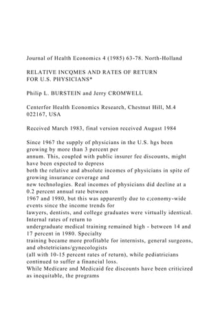
  • 13. Both of these patterns are clear in table 2 and fig. 1. In the latter, the solid vertical line which indicates the start of Medicare and Medicaid is not associated with any break in the earlier rising income trend. Over the first 68 P.L. Burstein and .I. Cromwell, U.S. physicians’ incomes 1980 $ 90,000 80,000 70,000 60,OOC 50,00( 40,001 30,oo d 1 Y L 1 53 55 57 59 61 63 65 67 69 71 73 75 77 79 80 Fig. 1. Real professional incomes, 1951430.
  • 14. P.L. Burstein and J. Cromwell, U.S. physicians’ incomes 69 part of the post-program period (1967-76), average physician income increased 1.1 percent per year. The second part of the post- program period (1972~80), on the other hand, saw on 0.8 percent per year real income decline. All three of our comparison groups - lawyers, dentists and male college graduates - also had real income declines between 1972 and 1980. (The income of high school graduates showed a similar pattern, with a 2.1 percent annual rate of increase followed by a -0.8 percent rate of decline.) The all-inclusive nature of the fall in real income indicates that some economy-wide phenomenon - probably the high and accelerating rate of inflation - was responsible for much, if not all, of the post- program decline in real physician incomes. The rehtive income situation is also interesting. Physician earnings were virtually constant between 1967-80 relative to the three comparison groups. The result vis-Lvis dentists is surprising, since the growth in dental insurance coverage was extremely rapid during this period3 while the supply of dentists was growing relatively more slowly (0.6 percent annual increase
  • 15. over the 1967-80 period versus 3.3 percent for physicians). It is quite possible that other, offsetting factors like the spread of fluoridation negated dentistry’s positive insurance effects, producing demand trends comparable with those of physicians experiencing slower insurance growth but more demand-inducing technical change, e.g., endoscopies, radionucleide and CAT scanning. There is nothing overt in the net income data that shows any impact of physician supply increases or deeper public insurance fee discounts on average physician incomes. This is a serious matter if it means that private financial incentives will not retard the current trend toward physician oversupply. Alternatively, if insurance and technology trends simply overwhelmed burgeoning supply effects in the 197Os, then the direct and indirect demand controls so prevalent in the 1980s (e.g., higher deductibles and copays) could have a material effect on future supplies. It has been demonstrated above that physicians are maintaining their relative and absolute income superiority over a sample of other professionals. Another and perhaps more important influence on the decision of potential new practitioners to enter the medical profession is the rate of financial return. This aspect 0; long-run physician supply is considered
  • 16. below. 3. Methodology for calculating rates of return As noted above, it is extremely difficult to draw any conclusions concerning rates of return to medical training from the existing literature. Years of analysis are limited in the individual studies, and no two estimates ‘The percentag e o f the U.S. population with private dental insurance rose from 3-23 percent 1967-77. 70 P.L. Burstein and J. Cromwell, U.S. physicians’ incomes are comparable. The present paper is unique in that a uniform approach is used to evaluate. rates of return, over a substantial period of time. 3.1. The basic formula Our basic rate of return Suppose that we wish to formula is taken from Sloan and Feldman (1978). compute the rate of return for group 2, which differs from the base group 1 primarily in that the former has undertaken an additional period of training. The present value Vi of the annual income Y1
  • 17. earned by group 1 (assuming that the income flow continues forever) is (1) where S1 is the first year of the income flow and tl is the appropriate discount rate for this group. Integrating this formula gives V, =(Y1/rl)e-‘IS1. (2) If group 2 spends more time in training than group 1, we can find the internal rate of return r to that investment by tinding the discount rate which equates V, to V,. This gives us (Y~/r)e-rSI=(Y,/r)e-‘S2, (3) which implies that YJY, =e’%-%). (4) Since, by definition, annual earnings Y equals the hourly wage W times the number of hours worked per year L for each pecuniary benefits are equal, our unadjusted becomes group, and assuming non- internal rate of return ); Eq. (5) is, of course, based on differences in annual earnings. If we assume that any gap between L, and L2 is induced by differences in the hou.rly wage
  • 18. and not any non-pecuniary benefits, then an equally valid formula would be ra=ln(KIK)/(S,-U, (6) where r, is interpreted as the hours-adjusted internal rate of return. If leisure has some value, and certain assumptions (see below) are satisfied, then the P.L. Burstein and J. Cromwell, U.S. physicians’ inc0me.s 71 true internal rate of return r to the additional training obtained by group 2 will lie somewhere between this hours-adjusted rate ra and r,. To demonstrate this, it is useful to make the additional assumption that the supply curve of labor is the same for the two groups and not perfectly inelastic. This implies that by voluntary choice, L2 >I,, in all relevant situations, ceteris paribus .4 For this extra labor time, group 2 will receive IV.,& -I,,) in additional earnings. However, not all of this earnings increment can be considered to be a true return. To obtain the extra money, group 2 individuals must give up (L, -IL,) hours of leisure. The net return to the extra work effort of group 2 is equal to the monetary return minus the value of the foregone leisure. Therefore, rates of return based on annual
  • 19. earnings unadjusted for differences in hours (e.g., P,) will overstate the actual benefit of belonging to group 2. Rates of return based on hourly earnings alone (e.g., r,J will understate the true rate of return, however, since some positive benefit must accrue to group 2 for the extra hours worked, for otherwise they would not have worked longer. Thus, if our basic formulas are correct, we may conclude that r,c~cr,. 3.2. Adjustments The rate of return formulas (5) and (6) are based on a number of implicit assumptions which would tend to cause inaccuracies when applied to the earnings of physicians. These assumptions include: -A constant length of physician training, -An equal (and infinite) work life for all groups, - Zero out-of-pocket educational costs for post-college training, -Zero earnings for medical residents, - Similar earnings/experience profiles for all groups. We made corrections for the first four of these, using the methods described below. We were unable to deal with the last item, so our rate of return estimates will be slight overestimates since the lifetime earnings advantage of physicians is concentrated somewhat in their later years. 3.2.1. Finite working lifetimes The first adjustment made to the basic formulas deals with the
  • 20. fact that workers do retire at a finite age. This means that the present value formula (1) represen ts an overestimate of actual discounted earnings. The error will be greater for those professions with the shortest working lives (or longest training). Our response was to reduce the & employed in the rate of return formulas by a factor of Vi/q, where v is retirement-adjusted present value 4We are assuming that the extra training has some monetary value. 72 P.L. Burstein and J. Cromwell, U.S. physicians* incomes of lifetime earnings, truncated at a fixed retirement age of 65 in (1). A discount rate of 10 percent was assumed. Perhaps contrary to a priori expectations, Vi/y varied from only 0.967 (physicians 1978) to 0.986 (college graduates). Potential earnings past age 65 are simply not of much importance to decisions made at age 21, due to the operation of the discount rate.5 This adjustment thus reduced the calculated rate of return to medical education by a maximum of 0.3 percentage points - an insignificant change as we shall see.
  • 21. This result is quite sensitive to the time discount rate employed. At a 5 percent rate, assuming a fixed, age 65 retirement rate for all occupations reduces the return to medical education by 2.3 percentage points. Unlike many college graduates, however, physicians enjoy a longer, more lucrative career which is ignored in using a 65 age limit. According to the latest AMA figures [AMA (1984)], 16.2 percent of GPs were still in active practice over age 65, working 45 hours per week, and enjoying a net income of $64,300 (compared to $116,500 for those in the peak earnings years, 46- 55). Without knowing exactly the true rate of time discount and recognizing the unequal retirement ages of college graduates and physicians, ail we can say is that the true adjustment probably lies somewhere between 0.3 and 2.3 percentage points. 3.2.2. Rising medical school costs Even with this adjustment, our rate of return formula does not take into account the out-of-pocket costs for more years of formal schooling. It is well known that medical school tuition rose sharply during the 197Os, from an average of $1,379 in 1970 to $5,287 in 1980 [Hadley (1980), JAMA (1983)]. Less well known, however, is the extraordinary rise in grants to medical
  • 22. students that took place over 1968-71 [Feldman (1980)], which caused a sharp decline in net annual tuition per medical student from approximately $2,200 to $1,700 per year (real 1967 dollars). The 1967 peak in real net tuition, in fact, was not surpassed until 1977, as the increase in grants almost exactly matched the rise in tuition over the 1971-75 period. To calculate the impact of these offsetting changes, the sum of the average net tuition over the four years of medical school was divided by the present value of total earnings for physicians to get a proportional reduction in the income figure to be used ‘in the rate of return formula. It was determined that net lifetime income was reduced approximately 2 percent when cost of education was taken into accotmt, resulting in a decline in the rate of return of close to 0.5 percentage points. ?his same point applies to the longer-thaz;avsrage working lives of physicians; the extra earnings from additional time in the labor force occur too far in the future to have any impact. A full year of extra earnings at age 66, for example, is discounted by a factor of 74 (from the viewpoint of a 21 year old with a 10 percent discount rate). P.L. Burstein and J. Cromwell, U.S. physicians’ incomes 73
  • 23. 3.63. Rising earnings of medical residents Finally, the substantial growth in earnings of physicians during their residency period ($15,000 per year, median, by 1979) were taken into account in similar fashion. The large increase in these earnings coupled with their timing early in a physician’s career made this an important factor. Calculated lifetime discounted earnings increased by between 2.6 to 8.8 percent under this adjustment at its peak (k977), with the specialties requiring longer training obviously benefiting the most from higher residency salaries. The average rate of return for all physicians relative to college students increased by 0.8 percentage points, while the rate of return for general surgeons (with the longest training/residency period) relative to general practitioners increased by 1.5 percentage points in 1977. 3.2.4. Net impact of adjustments The approximate net impacts of the three adjustments considered here were a 0.8 percentage point decrease in the calculated rate of return to a basic medical education, and a maximum 0.7 percentage point increase in the rate of return to specialized medical training. Both of these rates were lowered by the adjustments for finite working life (-0.3) and out-of-pocket costs of in-class ~
  • 24. training (-0.5), while the adjustment for the earnings of residents (+ 1.5) applied to the rate of return for specialists only. 4. Rates of return to physicians’ post-college training To compute the rate of return to post-college training, the incomes of physicians, dentists and lawyers were compared to those of college graduates. This is appropriate for dentists and lawyers since the decision to enter a professional school takes effect at the end of college, and no further decisions concerning investment in formal education must be made. For physicians, however, the choice of specialty made at the end of professional school vitally affects their future income and rate of return, as we shall show. Therefore, to calculate the rate of return to the first post-college training decision, i.e., to become a ‘doctor’, the impact of physician specialization must be deleted. This is achieved by computing rates of return for the group of physicians that did not undertake specialty training - the general practitioners. While the rate of return to all physician training was also calculated, it is the rate of return for general practitioners which is most comparable to the figures given for dentists and lawyers. Our results are given in table 3. They indicate that physicians, dentists and
  • 25. lawyers all earned a positive return on their post-college training. The adjusted rate of return for general practitioners was between 12.1 and 14.5 percent, and the unadjusted rate ranged from 16.3 to 19.0 percent. In P.L. Burstein and J. Cromwell, U.S. physicians’ incomes Table 3 Internal rates of return,” 1967-80. Year All physicians r. r” General practitioners r. rU Dentists Lawyersb r. rU rU 1980 1979 1978 1977 1976 1975 1974 1973
  • 26. 1972 1971 1970 1967 12.1% 14.0% 14.2% 11.6 13.7 14.5 11.0 13.2 13.0 10.2 12.6 13.3 10.5 13.3 12.4 11.6 14.2 12.3 12.0 14.3 14.5 10.8 13.8 12.5 10.7 14.2 12.2 11.6 15.1 13.2 11.8 14.7 12.1 11.3 14.3 12.5 11.7 15.5 13.2 16.7% 17.2 16.3 17.0 16.4 16.7 18.2 17.4 17.8 18.9 16.8 17.2 19.0 - - 7.2%
  • 27. 16.3% - 14.9% 7.2 6.8 - - 6.8 15.8 14.9 7.1 - - 7.1 14.9 14.8 7.1 - - 6.7 14.4 14.8 5.7 - - 6.6 16.1 15.7 7.0 - - 4.7 13.5 15.4 7.7 4; is the hours adjusted rate of return, and r, is the unadjusted rate. bNo ra was calculated for lawyers due to lack of data on hours of work for this group. . absolute terms, this was surely more than adequate to attract new entrants into the profession of medicine. In relative terms, the general practitioner’s rate was far superior to that of lawyers, and approximately equal to that of dentists. There is no indication of any major trend in the rate of return to initial post-college training for any of the professions. This is contrary to what we would expect if medical supply/demand factors had reduced physician incomes. The lower figure for the all-physician rate of return deserves some
  • 28. discussion. This pattern is almost certainly due to the movement toward increased specialization in the medical profession. If the marginal rate of return to medical education declines with additional years of training (which is in accordance with both investment theory and the figures presented in the next section), then increasing specialization must bring down the average rate of return for all physicians. It should be noted, however, that this average rate of return will have no impact on either the medical school or the specialization decision, which are affected only by the marginal return rates. Also note the difference between unadjusted and adjusted rates. The latter are lower, reflecting the longer average work weeks of physicians. On average the basic return to medical school is reduced about 4 points, or roughly 25 percent. This differential appears to be narrowing markedly over time, implying relative declines in physician work effort compared to other professionals. While consistent with the increase in the supply of physicians, P.L. Burstein and .?. Cromwell, U.S. physicians’ incomes 75 reduced work effort per physician makes the ability of the medical profession
  • 29. to keep their incomes up to previous standards even more difficult to explain unless major changes in practice organization and technology have improved their overall productivity. 5. Rates of return to some important specialties The groups chosen for study in this section are the general surgeons, obstetricians/gynecologists, internists and pediatricians. For calculating the rates of return to these specialists, general practitioners constitute our reference group. This is appropriate because the decision to enter a medical specialty can be taken only at the end of undergraduate medical training. Based on board-certification requirements, we assumed that general surgeons needed five years of post-medical school training, obstetricians/gynecologists four, and internists and pediatricians three.(j The results are given in table 4. Except for the pediatricians, specialization seems to have been highly profitable in the most recent years listed. Averaging the 1977-80 figures, internists Year Table 4 Internal rates of return to specialty training.” General Obstetricians-
  • 30. Internists surgeons gynecologists r, TU r, r, r, r, Pediatricians rU r, 1980 1979 1978 1977 1976 1975 1974 1973 1972 1971 1970 1969 1967 1955 1951 9.8% 11.3 11.4 11.2 8.9 6.3 10.3 13.3 E 12.5 ii:3 8.0 6.1 7.5 6.3 4.9 4.2 4.6 4.3 9.3 10.8 4.7 7.1
  • 31. 8.3 12.0 - n.a. - n.a. 13.6 11.3 12.5 10.6 11.9 10.6 10.8 9.4 12.5 11.5 11.6 il.2 9.1 8.1 9.2 10.2 8.8 9.1 8.8 9.1 11.2 11.2 9.7 9.1 7.4 6.8 6.2 n.a. 3.7 n.a. 14.8 14.0 14.2 11.4 9.5 8.4 11.5 10.0 13.0 10.3 12.1 10.5 11.7 9.7 10.2 9.2 9.3 7.6 9.1 6.3 11.8 10.0 8.4 7.3
  • 32. 7.5 8.0 10.0 n.a. 4.9 n.a. - - ii 3.0 - 2.3 - - - 2.0 2.4 ii - - 1.6 - 0.6 n.a. 4.1 n.a. 9, is the hours adjusted rate of return, and r, is the unadjusted rate. ‘-’ indicates a negative rate of return. “These figures were obtained from Wechsler (1976, table 1). Feldman (19gO) asserts that four years is a better estimate for a ‘typical’ internist, but he agrees with the other figures. The one year graduate medical education requirement for licensure has been ignored for GPs. 76 P.L. Burstein and J. Cromwell, U.S. physicians’ incomes received a rate of return of 10.6-11.3 percent, general surgeons 11.0-13.1 percent, and obstetricians 12.7-14.5 percent, while pediatricians suffered an
  • 33. income loss. 7 Going back to the years immediately following the introduction of Medicare and Medicaid (1967-69), we observe uniformly lower rates; internists received a rate of return between 9.6 and 6.5 percent, general surgeons 6.5-8.6 percent, obstetricians 7.7-8.0 percent, and pediatricians a negative return. Thus, except for pediatrics, the financial incentive to enter a specialty held up well in the post-program period. In fact, the rate of return to internists, general surgeons and obstetricians rose by 3.9, 4.5, and 5.8 percentage points, respectively, during this time. These increases represent a substantial fraction of the original return rates. It is interesting to note that the increased rates of return for the’ three profitable specialties cited here were not matched by an equivalent increase in the returns to general practitioners. Between 1967-69 and 1979-80 the GP rate of return rose by only 0.3 percentage points. Continuation of this trend for another decade would remove the general practitioner/specialty return rate differential completely. The movement toward increasing specialization has thus received added impetus from the private financial considerations of medical students. Pediatrics is obviously the exception; any individual entering this specialty must be strongly influenced by non-
  • 34. monetary considerations. 6. Conclusion The conventional picture of medicine as a financially attractive profession is strongly confirmed by this study. The difference in absolute incomes between physicians, on the one hand, and dentists and lawyers on the other was 35 and 139 percent, respectively, in 1978-80; this advantage will unquestionably remain large in the forseeable future. The internal rate of return to basic medical training exceeded 12 percent in every post-Medicare/Medicaid year, ‘ii:i;ng apprtiximatcly equal to that for dental education and roughly double the rate for law school. Medical specialization in the areas of internai medicine, general surgery and obstetrics/gynecology was also highly profitable, with the rates of return increasing substantially since the late 1960s. Pediatrics was the sole exception to this general picture of financial success, with decliuing birth rates and limited insurance perhaps being responsible for the negative rate of return to training in this specialty. (Their patients are ineligible for Medicare, and other insurers generally do not cover routine child care.) ‘The first number given for each speckity is the average af the
  • 35. 1977 and 1980 adjusted rates of return, and the second is the average of the unadjusted rates for the same years. It is not possible to exactly quantify any negative rate of return using the methods of this paper. P.L. Burstein and .l. Cromwell, U.S. physicians’ incomes 77 It is perhaps somewhat surprising that rates of return to medical training managed to stay so high in the face of (a) increasing fee discounts for public insurers, (b) rapidly growing physician supply, and (c) rising tuition costs. The first of these may be more apparent than real if physicians manipulate the ‘usual’ fees on which these discounts are calculated. Cromwell and Burstein (1982), for example, have shown that physicians only rarely receive full payment of their usual charge while Lee and Hadley (1981) demonstrate the po:;litive relationship between ‘usuals’ and usual- customary-reasonable payment m&hods as part of a revenue-maximizing game. Second, burgeoning supply could have been offset by increasing intensity per visit, which also is well documented for recent years (Cromwell et al. (1982), Freeland and Schendler (198l)J The third was shown to be counteracted by rising financial support for medical students, so that no significant increase in net
  • 36. medical school tuitio,1 was recorded over the 1967-80 period. The increase in the stipends of medical residents was a fourth factor, which was working to increase rates of return for specialty training substantially. One policy conclusion to emerge from the analysis is that programs designed to reduce total medical expenditures by limiting physician incomes can be enacted without serious impact on the financial attractiveness of this profession. Rates of return to medicine are not only high on an absolute basis, but equal or exceed those of other forms of post-graduate training. While non-pecuniary factors could explain the systematically higher returns (e.g., a distaste for the ‘sight of blood’, the long, arduous schooling), institutional rigidities probably explain the larger part of the differential. The ability of the profession to influence medical school admissions and licensure exams, as well as their resistance to legal delegation of more routine tasks to other health professionals, has certainly helped perpetuate their economic advantage [Sloan (1970), Frech (1974), Kessel(l970)]. Another conclusion points to the ‘hidden subsidy’ afforded physicians by all insurers, including Medicare and Medicaid. Increased insurance coverage has enhanced returns not only by raising the demand of the elderly and the
  • 37. poor, but by increasing the remuneration of residents via cost- based reimbursement of teaching hospitals. Since only specialists in training receive the benefits of this change, this could be one of the important factors behind the enhanced rates of return for specialty training. Given the enormous financial advantage to a medical education, insurers might reconsider their policy of including resident salaries as a fully allowable expense. References American Medical Association, 1973, Measuring physician manpower: Contritiutiorss to a comprehensive health manpower strategy (Center for Health Services Research and Develop- ment, Chicago, IL). American Medical Association, 1984, The American health care system. 78 P.L. Burstein and J. Cromwell, U.S. physicians’ incomes Cromwell, Jerry and Philip L. Burstein, 1982, Physician losses from Medicare/Medicaid participation: How real are they? (Center for Health Economics Research, Chestnut Hill, MA). Cromwell, Jerry, J. Mitchell and P. Burstein, 1982, Analysis of changes in the content of
  • 38. physician office visits: Descriptive analysis of NAMCS, Report to DHHS/HRA, contract no. 232-81-0039. Dresch, Stephen P., 1981, Marginal wage rates, hours of work and returns to physician specialization, in: Nancy Greenspan, ed., Issues in physician reimbursement: Health care linancing conference proceedings, DHHS publication no. (HCFA) 03121 (Department of Health and Human Services, Washington, DC) 165-200. Feldman, Roger D., 1980, Loan programs and medical education financing in: Jack Hadley, ed., Medical education financing (Neale Watson, New York) 94-127. Feldman, Roger D. and R.M. Scheffler, 1976, The supply of medical school applicants and the rate of return to training (Economics Department, University of North Carolina, Chapel Hill, NC). Frech, H.E., 1974, Occupational licensure and health care productivity: The issues and the literature, in: J. Rafferty, ed., Health manpower and productivity (Heath, Lexington, MA) 119-142. Freeland, Mark S. and C. Schendler, 1981, National health expenditures: Short-term outlook and long-term projections, Health Care Financing Review 2,97- 138. Goldstein, Marcus S., 1972, Income of physicians, osteopaths and dentists from professional practice, 196569, DHEW publication no. (SSA) 73-11852
  • 39. (Department of Health Education and Welfare, Washington, DC). Hadley, Jack, 1980, Introduction, in: Jack Hadley, ed., Medical education financing (Neale Watson, New York) l-22. Hough, Douglas, 1981, The economic status of resident physicians, in: David Goldfarb, ed., Profile of medical practice (American Medical Association, Monroe, WI) 83-96. Journal of the American Medical Association, 1983,83rd Annual report on me&al education in the U.S. Kessel, Reuben A., 1970, The AMA and the supply of physicians, Law and contemporary problems, Health Care 35, no. 2, Part I, 267-283. Kniesner, T.J., 1976, An indirect test of complementarity in the family labor supply model, Econometrica 34,651-670. Langwell, Kathryn M., 1982, Sex differences in returns to physicians’ choice of specialty, Journal of Health Politics, Policy and Law 7, 752-761. Lee, Robert and J. Hadley, 1981, Physicians’ fees and public medical care programs, Health Services Research 16, 185-203. Lindsay, Cotton M., 1973, Real returns to medical education, Journal of Human Resources 8, 331-348.
  • 40. Mennemeyer, Stephen T., 1978, Really great returns to medical education, Journal of Human Resources 13,75-90. Mitchell. Janet B. et al., 1981, Physician participation in public programs (Center for Health Economics Research, Chestnut Hill, MA). Sloan, Frank A., 1970, Lifetime earnings and physicians’ choice of specialty, Industrial and Labor Relations Review 24, 49. Sloan, Frank A. and Roger Feldman, 1978, Competition among physicians, in: Warren Greenberg, ed., Competition in the health care sector: Past, present, and future, Proceedings of a conference sponsored by the Bureau of Economics, FTC, 57-131. Wechsler, Henry, 1976, Handbook of medical specialties (Human Services Press, New York). On the Concept of Health Capital and the Demand for Health Michael Grossman National Bureau of Economic Research The aim of this study is to construct a model of the demand for the commodity ''good health." The central proposition of the model is that health can be viewed as a durable capital stock that produces an
  • 41. output of healthy time. It is assumed that individuals inherit an initial stock of health that depreciates with age and can be increased by investment. In this framework, the "shadow price" of health depends on many other variables besides the price of medical care. It is shown that the shadow price rises with age if the rate of depreciation on the stock of health rises over the life cycle and falls with education if more educated people are more efficient producers of health. Of particular importance is the conclusion that, under certain conditions, an increase in the shadow price may simultaneously reduce the quantity of health demanded and increase the quantity of medical care demanded. I. Introduction During the past two decades, the notion that individuals invest in them- selves has become widely accepted in economics. At a conceptual level, increases in a person's stock of knowledge or human capital are assumed to raise his productivity in the market sector of the economy, where he produces money earnings, and in the nonmarket or household sector, where he produces commodities that enter his utility function. To realize
  • 42. This paper is hased on part of my Columbia University Ph.D. dissertation, "The Demand for Health: A Theoretical and Empirical Investigation," which will be pub- lished by the National Bureau of Economic Research. My research at the Bureau was supported by the Commonwealth Fund and the National Center for Health Services Research and Development (PHS research grant 2 P 01 HS 00451-04). Most of this paper was written while I was at the University of Chicago's Center for Health Ad- ministration Studies, with research support from the National Center for Health Ser- vices Research and Development (PHS grant HS 00080). A preliminary version of this paper was presented at the Second World Congress of the Econometric Society. I am grateful to Gary S. Becker, V. K. Chetty, Victor R. Fuchs, Gilbert R. Ghez, Robert T. Michael, and Jacob Mincer for their helpful comments on earlier drafts. 2 2 4 JOURNAL OF POLITICAL ECONOMY potential gains in productivity^ individuals have an incentive to invest in formal schooling or in on-the-job training. The costs of these invest- ments include direct outlays on market goods and the opportunity cost of the time that must be withdrawn from competing uses. This frame- work has been used by Becker (1967) and by Ben-Porath (1967)
  • 43. to develop models that determine the optimal quantity of investment in human capital at any age. In addition, these models show how the optimal quantity varies over the life cycle of an individual and among individuals of the same age. Although several writers have suggested that health can be viewed as one form of human capital (Mushkin 1962, pp. 129-49; Becker 1964, pp. 33-36; Fuchs 1966, pp. 90-91), no one has constructed a model of the demand for health capital itself. If increases in the stock of health simply increased wage rates, such a task would not be necessary, for one could simply apply Becker's and Ben-Porath's models to study the decision to invest in health. This paper argues, however, that health capital differs from other forms of human capital. In particular, it argues that a person's stock of knowledge affects his market and nonmarket productivity, while his stock of health determines the total amount of time he can spend producing money earnings and commodities. The fundamental difference between the two types of capital is the basic justification for the model of the demand for health that is presented in the paper. A second justification for the model is that most students of
  • 44. medical economics have long realized that what consumers demand when they purchase medical services are not these services per se but, rather, '̂ good health." Given that the basic demand is for good health, it seems logical to study the demand for medical care by first constructing a model of the demand for health itself. Since, however, traditional demand theory assumes that goods and services purchased in the market enter consumers' utihty functions, economists have emphasized the demand for medical care at the expense of the demand for health. Fortunately, a new approach to consumer behavior draws a sharp distinction between fundamental ob- jects of choice—called ^'commodities'^-—and market goods (Becker 1965; Lancaster 1966; Muth 1966; Michael 1969; Becker and Michael 1970; Ghez 1970). Thus, it serves as the point of departure for my health model. In this approach, consumers produce commodities with inputs of market goods and their own time. For example, they use traveling time and transportation services to produce visits; part of their Sundays and church services to produce ''peace of mind"; and their own time, books, and teachers' services to produce additions to knowledge. Since goods and services are inputs into the production of commodities, the
  • 45. demand for these goods and services is a derived demand. Within the new framework for examining consumer behavior, it is assumed that individuals inherit an initial stock of health that depreciates CONCEPT OF HEALTH CAPITAL 225 over time—at an increasing rate, at least after some stage in the life cycle—and can be increased by investment. Death occurs when the stock falls below a certain level, and one of the novel features of the model is that individuals **choose" their length of life. Gross investments in health capital are produced by household production functions whose direct inputs include the own time of the consumer and market goods such as medical care, diet, exercise, recreation, and housing. The produc- tion function also depends on certain '^environmental variables," the most important of which is the level of education of the producer, that influence the efficiency of the production process. It should be realized that in this model the level of health of an indi- vidual is not exogenous but depends, at least in part, on the resources
  • 46. allocated to its production. Health is demanded by consumers for two reasons. As a consumption commodity, it directly enters their preference functions, or, put differently, sick days are a source of disutility. As an investment commodity, it determines the total amount of time available for market and nonmarket activities. In other words, an increase in the stock of health reduces the time lost from these activities, and the mone- tary value of this reduction is an index of the return to an investment in health. Since the most fundamental law in economics is the law of the down- ward-sloping demand curve, the quantity of health demanded should be negatively correlated with its shadow price. The analysis in this paper stresses that the shadow price of health depends on many other variables besides the price of medical care. Shifts in these variables alter the optimal amount of health and also alter the derived demand for gross investment, measured, say, by medical expenditures. It is shown that the shadow price rises with age if the rate of depreciation on the stock of health rises over the life cycle and falls with education if more educated people are more efficient producers of health. Of particular importance is
  • 47. the conclusion that, under cwtain conditions, an increase in the shadow price may simultaneously reduce the quantity of health demanded and increase the quantity of medical care demanded. n . A Stock Approach to the Demand for Health A, The Model Let the intertemporal utility function of a typical consumer be U = U(<f>ono, . . . , <f>nHn, ZQJ , . . , Zn), ( 1 ) where Ho is the inherited stock of health. Hi is the stock of health in the iih time period, <t>i is the service flow per unit stock, hi = </>ifl"̂ is total consumption of "health services," and Z^ is total consumption of another 2 2 6 JOURNAL OF POLITICAL ECONOMY commodity in the ith period.^ Note that, whereas in the usual inter- temporal utility function «, the length of life as of the planning date, is fixed, here it is an endogenous variable. In particular, death takes place when Hi = Hmin- Therefore, length of life depends on the quantities of Hi that maximize utility subject to certain production and resource con- straints that are now outlined.
  • 48. By definition, net investment in the stock of health equals gross invest- ment minus depreciation: Hi^^~Hi^h-h,H,, (2) where Ii is gross investment and 8̂ is the rate of depreciation during the fth period. The rates of depreciation are assumed to be exogenous, but they may vary with the age of the individual.^ Consumers produce gross investments in health and the other commodities in the utility function according to a set of household production functions: (3) In these equations, Mi is medical care, Xi is the goods input in the pro- duction of the commodity Z ,̂ THi and Ti are time inputs, and Ei is the stock of human capital.^ It is assumed that a shift in human capital changes the efficiency of the production process in the nonmarket sector of the economy, just as a shift in technology changes the efficiency of the production process in the market sector. The implications of this treat- ment of human capital are explored in Section IV. It is also assumed that all production functions are homogeneous of degree 1 in the goods and time inputs. Therefore, the gross
  • 49. investment production function can be written as (4) where ti ^= THi/Mi. It follows that the marginal products of time and medical care in the production of gross investment in health are 1 The commodity Z,- may be viewed as an aggregate of all commodities besides health that enter the utility function in period i. For the convenience of the reader, a glossary of symbols may be found in Appendix B. 2 In a more complicated version of the model, the rate of depreciation might be a negative function of the stock of health. The analysis is considerably simplified by treating this rate as exogenous, and the conclusions reached would tend to hold even if it were endogenous. 3 In general, medical care is not the only market good in the gross investment func- tion, for inputs such as housing, diet, recreation, cigarette smoking, and alcohol con- sumption influence one*s level of health. Since these inputs also produce other commodities in the utility function, joint production occurs in the household. For an analysis of this phenomenon, see Grossman (1970, chap. 6). To emphasize the key aspects of my health model, I treat medical care as the most important market good in the gross investment function in the present paper.
  • 50. CONCEPT OF HEALTH CAPITAL 2 2 7 (5) From the point of view of the individual, both market goods and own time are scarce resources. The goods budget constraint equates the present value of outlays on goods to the present value of earnings income over the life cycle plus initial assets (discounted property income):^ W,TW, = 2. ^ + ^0- (6) Here Pi and Vi are the prices of Mi and Xi^ W^ is the wage rate, TWi is hours of workj ^o is discounted property income, and r is the interest rate. The time constraint requires that Q, the total amount of time available in any period, must be exhausted by all possible uses: TW, + TL, + TH, + T,= Q, (7) where TLi is time lost from market and nonmarket activities due to illness or injury. Equation (7) modifies the time budget constraint in Becker's time model (Becker 1965). If sick time were not added to market and non-
  • 51. market time, total time would not be exhausted by all possible uses. My model assumes that TL, is inversely related to the stock of health; that is, 'dTLi/'^Hi < 0. If Q were measured in days (Q = 365 days if the year is the relevant period) and if <f>i were defined as the flow of healthy days per unit of Hi, h-, would equal the total number of healthy days in a given year.^ Then one could write TL, = Q-h. (8) It is important to draw a sharp distinction between sick time and the time input in the gross investment function. As an illustration of this difference, the time a consumer allocates to visiting his doctor for periodic checkups is obviously not sick time. More formally, if the rate of de- preciation were held constant, an increase in TH.i would increase U and Hij^i and would reduce TL^^i. Thus, TH, and TZ^+i would be negatively correlated.® ^ The sums throughout this study are taken from f r= 0 to n. 5 If the stock of health yielded other services besides healthy days, 0̂ would be a vector of service flows. This study emphasizes the service flow of healthy days because this flow can be measured empirically.
  • 52. 6 For a discussion of conditions that would produce a positive correlation between and TL^_^_^, see Section III. 2 2 8 JOURNAL OF POLITICAL ECONOMY By substituting for TWi from equation (7) into equation ( 6 ) , one obtains the single '*full wealth'' constraint: + V,X, + W,{TL, + TH, + (9) According to equation ( 9 ) , full wealth equals initial assets plus the present value of the earnings an individual would obtain if he spent all of his time at work. Part of this wealth is spent on market goods, part of it is spent on nonmarket production time, and part of it is lost due to illness. The equilibrium quantities of Hi and Zi can now be found by maximizing the utility function given by equation (1) subject to the constraints given by equations ( 2 ) , ( 3 ) , and (9).'' Since the inherited stock of health and the rates of depreciation are given, the optimal quantities of gross investment determine the optimal quantities of health capital. B. Equilibrium Conditions
  • 53. First-order optimality conditions for gross investment in period i — 1 Uhn + . .. + (1 - 8,) ... (1 - K_y) -Y-Gn, (10) 11 The new symbols in these equations are: Vhi ^ "dUfdh; =: the marginal utility of healthy days; ^ = the marginal utihty of wealth; Gi- ^'dhi/ i) = the marginal product of the stock of health in the production of healthy days; and :itt_i = the marginal cost of gross investment in health in period i — 1. "̂ In addition, the constraint is imposed that H^ ^ ^miir 8 Note that an increase in gross investment in period i — 1 increases the stock of health in all future periods. These increases are equal to dHi _ _ For a derivation of equation (10), see Part A of the Mathematical Appendix. CONCEPT OF HEALTH CAPITAL 2 2 9 Equation (10) simply states that the present value of the marginal cost of gross investment in period i — 1 must equal the present
  • 54. value of marginal benefits. Discounted marginal benefits at age / equal I J where Gi is the marginal product of health capital—the increase in the number of healthy days caused by a one-unit increase in the stock of health. Two monetary magnitudes are necessary to convert this marginal product into value terms, because consumers desire health for two reasons. The discounted wage rate measures the monetary value of a one- unit in- crease in the total amount of time available for market and nonmarket activities, and the term Uh.i/X measures the discounted monetary equiva- lent of the increase in utihty due to a one-unit increase in healthy time. Thus, the sum of these two terms measures the discounted marginal value to consumers of the output produced by health capital. While equation (10) determines the optimal amount of gross invest- ment in period i— 1, equation (11) shows the condition for minimizing the cost of producing a given quantity of gross investment. Total cost is minimized when the increase in gross investment from spending an additional dollar on medical care equals the increase in gross investment from spending an addidonal dollar on time. Since the gross
  • 55. investment production function is homogeneous of degree 1 and since the prices of medical care and time are independent of the level of these inputs, the average cost of gross investment is constant and equal to the marginal cost. To examine the forces that affect the demand for health and gross in- vestment, it is useful to convert equation (10) into a slightly different form. If gross investment in period i is positive, then . _ i+id^i ( i 4 i ) i + 2 i + 2 / • * l ^ I 1 ' / . • • . * t O I ' " * (l+r) Ov _i -I ) ( 1 O« 1 ) vV«( r-. — . (12) From (10) and ( 1 2 ) , ( l - l ( l + ; - ) i - i " (14-ry + ~ I ~ " ^ Therefore, (13) )
  • 56. 2 3 0 JOURNAL OF POLITICAL ECONOMY where JCi_i is the percentage rate of change in marginal cost between period i— 1 and period i.^ Equation (13) implies that the undiscounted value of the marginal product of the optimal stock of health capital at any moment in time must equal the supply price of capital, 7ti^i{r — jCi_i + 6 0 . The latter contains interest, depreciation, and capital gains components and may be interpreted as the rental price or user cost of health capital. Condition (13) fully determines the demand for capital goods that can be bought and sold in a perfect market. In such a market, if firms or households acquire one unit of stock in period i— 1 at price Jti_i, they can sell (1 — hi) units at price Tti at the end of period i. Consequently, jt£_i(r — Jti_i + 8,) measures the cost of holding one unit of capital for one period. The transaction just described allows individuals to raise their capital in period / alone by one unit and is clearly feasible for stocks like automobiles, houses, refrigerators, and producer durables. It suggests that one can define a set of single-period flow equilibria for stocks that last for many periods.
  • 57. In my model, the stock of health capital cannot be sold in the capital market, just as the stock of knowledge cannot be sold. This means that gross investment must be nonnegative. Although sales of health capital are ruled out, provided gross investment is positive, there exists a used cost of capital that in equilibrium must equal the value of the marginal product of the stock.̂ *̂ An intuitive interpretation of this result is that exchanges over time in the stock of health by an indiadual substitute for exchanges in the capital market. Suppose a consumer desires to increase his stock of health by one unit in period i. Then he must increase gross investment in period i — 1 by one unit. If he simultaneously reduces gross investment in period i hy (1 — 8̂ ) units, then he has engaged in a transaction that raises Hi and Hi alone by one unit. Put differently, he has essentially rented one unit of capital from himself for one period. The magnitude of the reduction in It is smaller the greater the rate of depreciation, and its dollar value is larger the greater the rate of increase in marginal cost over time. Thus, the depreciation and capital gains components are as relevant to the user cost of health as they are to the user cost of any other durable. Of course, the interest component of user cost is easy to
  • 58. interpret, for if one desires to increase his stock of health rather than his stock of some other asset by one unit in a given period, rjt^_i measures the interest payment he '^Equation (13) assumes S/5t-_j ^ 0 . 10 For similar conclusions with regard to nonsalable physical capital and with regard to a nonsalable stock of ^'goodwill" produced by advertising, see Arrow (1968) and Nerlove and Arrow (1962). 11 In a continuous time model, the user cost of health capital can be derived in one step. If continuous time is employed, the term b^Ki_^ does not appear in the user cost formula. The right-hand side of (13) becomes Jt^(r — jt̂ + 6^), where K, is the in- CONCEPT OF HEALTH CAPITAL 2 3 1 A slightly different form of equation (13) emerges if both sides are divided by the marginal cost of gross investment: ^ i, (13') Here Yi = {WiGi)/Ki_i is the marginal monetary rate of return on an investment in health and
  • 59. Uh, is the psychic rate of return. In equilibrium, the total rate of return on an investment in health must equal the user cost of health capital in terms of the price of gross investment. The latter variable is defined as the sum of the real-own rate of interest and the rate of depreciation. C. The Pure Investment Model It is clear that the number of sick days and the number of healthy days are complements; their sum equals the constant length of the period. From equation (8), the marginal utility of sick time is —Uhi, Thus, by putting healthy days in the utility function, one implicitly assumes that sick days yield disutility. If healthy days did not enter the utility function directly, the marginal monetary rate of return on an investment in health would equal the cost of health capital, and health would be solely an in- vestment commodity.^- In formalizing the model, I have been reluctant to treat health as pure investment because many observers believe the demand for it has both investment and consumption aspects (see, for example, Mushkin 1962, p. 131; Fuchs 1966, p. 86). But to simplify the remainder of the theoretical analysis and to contrast health capital with
  • 60. other forms of human capital, the consumption aspects of demand are ignored from now on.̂ ^ If the marginal utility of healthy days or the marginal disutility of sick days were equal to zero, condition (13') for the optimal amount of health capital in period i would reduce to i. ( 1 4 ) stantaneous percentage rate of change of marginal cost at age i. For a proof, see Part B of the Mathematical Appendix. 12 To avoid confusion, a note on terminology is in order. If health were entirely an investment commodity, it would yield monetary, but not utility, returns. Regardless of whether health is investment, consumption, or a mixture of the two, one can speak of a gross investment function since the commodity in question is a durable. 13 Elsewhere, I have used a pure consumption model to interpret the set of phenom- ena that are analyzed in Sections III and IV. In the pure consumption model, the marginal monetary rate of return on an investment in health is set equal to zero (see Grossman 1970, chap. 3). 232 JOURNAL OF POLITICAL ECONOMY
  • 61. Equation (14) can be derived explicitly by excluding health from the utility function and by redefining the full wealth constraint as^^ ' = 0̂ + (15) Maximization of R' with respect to gross investment in periods i — 1 and i yields + (1 -f (16) + ...+ (1 — ( 1 - 8 0 . . . (1 - K- (17) These two equations imply that (14) must hold. Figure 1 illustrates the determinations of the optimal stock of health capital at any age i. The demand curve MEC shows the relationship between the stock of health and the rate of return on an investment or the marginal efficiency of health capital, yi- The supply curve S shows the relationship between the stock of health and the cost of capital, r — Si_i - j - 6i. Since the cost of capital is independent of the stock, the
  • 62. supply curve is infinitely elastic. Provided the MEC schedule slopes downward, F I G . 1 Since the gross investment production function is homogeneous of the first degree, CONCEPT OF HEALTH CAPITAL 233 365 FIG. 2 the equilibrium stock is given by Hi^j where the supply and demand curves intersect. In the model, the wage rate and the marginal cost of gross investment do not depend on the stock of health. Therefore, the MEC schedule would be negatively inclined if and only if G ,̂ the marginal product of health capital, were diminishing. Since the output produced by health capital has a finite upper limit of 365 healthy days, it seems reasonable to assume diminishing marginal productivity. Figure 2 shows a plausible relation- ship between the stock of health and the number of healthy days. This relationship may be called the "production function of healthy
  • 63. days." The slope of the curve in the figure at any point gives the marginal product of health capital. The number of healthy days equals zero at the death stock ^min, so that Q = TLi ^ 3 6 5 is an alternative definition of death. Beyond ^min, healthy time increases at a decreasing rate and eventually approaches its upper asymptote of 365 days as the stock becomes large. In Sections I I I and IV, equation (14) and figure 1 are used to trace out the lifetime path of health capital and gross investment, to explore the effects of variations in depreciation rates, and to examine the impact of changes in the marginal cost of gross investment. Before I turn to these matters, some comments on the general properties of the model are in order. It should be realized that equation (14) breaks down whenever desired gross investment equals zero. In this situation, the present value of the marginal cost of gross investment would exceed the present value of marginal benefits for all positive quantities of gross investment, and equations (16) and (17) would be replaced by inequalities.^^ The re- mainder of the discussion rules out zero gross investment by assumption, but the conclusions reached would have to be modified if this were not
  • 64. the case. One justification for this assumption is that it is observed em- pirically that most individuals make positive outlays on medical care throughout their life cycles. h~i = h =15 Formally, ŷ ̂ ^ — Jtf_i + 2 3 4 JOURNAL OF POLITICAL ECONOMY Some persons have argued that, since gross investment in health cannot be nonnegative, equilibrium condition (14) should be derived by using the optimal control techniques developed by Pontryagin and others. Arrow (1968) employs these techniques to analyze a firm's demand for non- salable physical capital. Since, however, gross investment in health is rarely equal to zero in the real world, the methods I use— discrete time maximization in the text and the calculus of variations in the Mathe- matical Appendix—are quite adequate. Some advantages of my methods are that they are simple, easy to interpret, and familiar to most econo- mists. In addition, they generate essentially the same equilibrium condition as the Pontryagin method. Both Arrow and I conclude that, if desired gross investment were positive, then the marginal efficiency of nonsalable
  • 65. capital would equal the cost of capital. On the other hand, given zero gross investment, the cost of capital would exceed its marginal efficiency. The monetary returns to an investment in health differ from the returns to investments in education, on-the-job training, and other forms of human capital, since the latter investments raise wage rates.^^ Of course, the amount of health capital might infiuence the wage rate, but it necessarily influences the time lost from all activities due to illness or injury. To emphasize the novelty of my approach, I assume that health is not a determinant of the wage rate. Put differently, a person's stock of knowl- edge affects his market and nonmarket productivity, while his stock of health determines the total amount of time he can spend producing money earnings and commodities. Since both market time and nonmarket time are relevant, even individuals who are not in the labor force have an incentive to invest in their health. For such individuals, the marginal product of health capital would be converted into a dollar equivalent by multiplying by the monetary value of the marginal utility of time. Since there are constant returns to scale in the production of gross
  • 66. investment and since input prices are given, the marginal cost of gross investment and its percentage rate of change over the life cycle are exogenous variables. In other words, these two variables are independent of the rate of investment and the stock of health. This implies that con- sumers reach their desired stock of capital immediately. It also implies that the stock rather than gross investment is the basic decision variable in the model. By this I mean that consumers respond to changes in the cost of capital by altering the marginal product of health capital and not the marginal cost of gross investment. Therefore, even though equation (14) is not independent of equations (16) and (17), it can be used to determine the optimal path of health capital and, by implication, the optimal path of gross investment.^''' difference is emphasized by Mushkin (1962, pp. 132-33). 1*̂ This statement is subject to the modification that the optimal path of capital must always imply nonnegative gross investment. CONCEPT OF HEALTH CAPITAL 235 Indeed, the major differences between my health model and the human
  • 67. capital models of Becker (1967) and Ben-Porath (1967) are the assump- tions made about the behavior of the marginal product of capital and the marginal cost of gross investment. Both Becker and Ben-Porath assume that any one person owns only a small amount of the total stock of human capital in the economy. Therefore, the marginal product of his stock is constant. To rule out solutions in which the desired stock of capital is either zero or infinite, they postulate that the marginal cost of producing gross additions to the stock is positively related to the rate of gross investment. Since marginal cost rises, the desired stock of human capital is not reached immediately. Moreover, since the marginal product of capital is constant, gross investment is the basic decision variable in these models.^^ In my model, on the other hand, the marginal product of health capital falls because the output produced by this capital has a finite upper limit. Consequently, it is not necessary to introduce the assumption of rising marginal cost in order to determine the optimal stock. To illustrate how the implications of the health and human capital models differ, suppose the rate of depreciation on either the stock of health
  • 68. or human capital rises. This upsets the equality between the cost of capital and its marginal efficiency. To restore this equality in the health model, the marginal product of health capital must rise, which would occur only if the stock of capital declines. To restore this equality in the human capital model, marginal cost must fall, which is possible only if gross investment declines.^^ HL Life Cycle Variations in Depreciation Rates Equation (14) enables one to study the behavior of the demand for health and gross investment over the life cycle. To simplify the analysis, it is assumed that the wage rate, the stock of knowledge, the marginal cost of gross investment, and the marginal productivity of health capital are independent of age. These assumptions are not as restrictive as they may seem. To be sure, wage rates and human capital are undoubtedly cor- related with age, but the effects of shifts in these variables are treated in Section IV. Therefore, the results obtained in this section may be viewed as partial effects. That is, they show the impact of a pure increase in age on the demand for health, with all other variables held constant. IS For a complete discussion of these points, see Becker (1967, pp. 5-12) and Ben-
  • 69. Porath (1967, pp. 353-61). For models of the demand for physical capital by firms in which the marginal cost of investment and the amount of investment are positively correlated, see, for example, Eisner and Strotz (1963) and Gould (1968). 1^ Section I I I demonstrates that an increase in the rate of depreciation on health capital might cause gross investment to increase. 236 JOURNAL OF POLITICAL ECONOMY Since marginal cost does not depend on age, Jti_i — 0 and equation (14) reduces to K (18) It is apparent from equation (18) that, if the rate of depreciation were independent of age, a single quantity of H would satisfy the equality between the marginal rate of return and the cost of health capital. Con- sequently, there would be no net investment or disinvestment after the initial period. One could not, in general, compare ^ 0 and H^ because accumulation in the initial period would depend on the discrepency be- tween the inherited stock and the stock desired in period 1. This dis- crepency in turn would be related to variations in H^y and other
  • 70. variables across individuals. But, given zero costs of adjusting to the desired level immediately, H would be constant after period 1. Under the stated condition of a constant depreciation rate, individuals would choose an infinite life if they choose to hve beyond period 1. In other words, if Hx > ^min? then Hi would always exceed the death stock.-^ To permit the demand for health to vary with age, suppose the rate of depreciation depends on age. In general, any time path of hi is possible. For example, the rate of depreciation might be negatively correlated with age during the early stages of the life cycle. Again, the time path might be nonmonotonic, so that hi rises during some periods and falls during others. Despite the existence of a wide variety of possible time paths, it is ex- tremely plausible to assume that 6̂ is positively correlated with age after some point in the life cycle. This correlation can be inferred because, as an individual ages, his physical strength and memory capacity deteriorate. Surely, a rise in the rate of depreciation on his stock of health is merely one manifestation of the biological process of aging. Therefore, the anal- ysis focuses on the effects of an increase in the rate of depreciation with age.
  • 71. Since a rise in 8̂ causes the supply curve of health capital to shift up- ward, it would reduce the quantity of health capital demanded over the life cycle. Graphically, an increase in the cost of capital from r --hi to r-|-8.i_|_i in figure 3 reduces the optimal stock from Hi to i^i+i. The greater the elasticity of the MEC schedule, the greater the decrease in the optimal stock with age. Put differently, the slower the increase in the marginal product of health capital as H falls, the greater the decrease in the optimal stock. Differentiation of equation (18) with respect to age quantifies the percentage rate of decrease in the stock of health over the life cycle: (19) -0 The possibility that death can occur in period 1 is ruled out from now on. CONCEPT OF HEALTH CAPITAL 237 r + 5 F I G . 3 In this equation, the tilde notation denotes a percentage time
  • 72. derivative {Hi^= (dHi/di) (I/Hi), etc.), and the new symbols are: 5̂ = 6i/ 8 := the share of depreciation in the cost of health capital and d nHi — —d e.,- = — the elasticity of the MEC schedule (In stands for natural logarithm).^^ Equation (19) indicates that the absolute value of the percentage de- crease in H is positively related to the elasticity of the MEC schedule, the share of depreciation in the cost of health capital, and the percentage rate of increase in the rate of depreciation. If ê and 8,- were constant, the curve relating In Hi to age would be concave unless r = 0, s i ^ ^ (20) di The absolute value of Hi increases over the life cycle because depre- ciation's share in the cost of capital rises with age. 21 From equation (18), ln(r + 6 )̂ =nW + ]D.G^ — In JT. Therefore, 8.- 8a H, or -2 Differentiation of (19) with respect to age yields
  • 73. or 2 3 8 JOURNAL OF POLITICAL ECONOMY If 8; grows continuously with age after some point in the life cycle, persons would choose to live a finite life. Since H declines over the life cycle, it would eventually fall to i?min, the death stock. When the cost of health capital is r + 8n in figure 3, Hn — Hmin, and death occurs. At death, no time is available for market and nonmarket activities, since healthy time equals zero. Therefore, the monetary equivalent of sick time in period n would completely exhaust potential full earnings, Wn^- More- over, consumption of the commodity Zn would equal zero, since no time would be available for its production if total time equals sick time.̂ -̂ Be- cause individuals could not produce commodities, total utility would be driven to zero at death.-^ Having characterized the optimal path of H,, one can proceed to ex- amine the behavior of gross investment. Gross investment's life cycle profile would not, in general, simply mirror that of health capital. In other words, even though health capital falls over the life cycle,
  • 74. gross investment might increase, remain constant, or decrease. This follows because a rise in the rate of depreciation not only reduces the amount of health capital demanded by consumers but also reduces the amount of capital supplied to them by a given amount of gross investment. If the change in supply exceeded the change in demand, individuals would have an incentive to close this gap by increasing gross investment. On the other hand, if the change in supply were less than the change in demand, gross investment would tend to fall over the life cycle. To predict the effect of an increase in hi with age on gross investment, note that the net investment can be approximated by HiHir'' Since gross investment equals net investment plus depreciation. (21) Differentiation of equation (21) with respect to age yields + hiHi + Hu + 8A rii + Oi Suppose hi and ê were constant. Then from (19) and ( 2 0 ) , the expres- sion for Ii would simplify to 23 The above s t a t e m e n t assumes t h a t Z- cannot be
  • 75. produced with X^ alone. This would be true if, say, the production function were Cobb- Douglas. 24 Utility equal zero when H = ^nijn provided the death time utiUty function is such t h a t U{0) = 0 . 25 T h a t is, TJ TJ TJ ' U TJ dt Hi The use of this approximation essentially allows one to ignore the one-period lag be- tween a change in gross investment and a change in the stock of health. CONCEPT OF HEALTH CAPITAL 239 7 8(1 — ̂ ê) (hi — f Since health capital cannot be sold, gross investment cannot be nega- tive. Therefore, hi ^ —Hi.̂ ^ That is, if the stock of health falls over the life cycle, the absolute value of the percentage rate of net disinvestment cannot exceed the rate of depreciation. Provided gross investment does not equal zero, the term 8̂ — SiSb in equation (22) must exceed zero. It follows that a sufficient condition for gross investment to be
  • 76. positively correlated with the depreciation rate is e < l/si. Thus, Ii would definitely be positive at every point if 8 < 1. The important conclusion is reached that, if the elasticity of the MEC schedule were less than 1, gross investment and the depreciation rate would be positively correlated over the life cycle, while gross investment and the stock of health would be negatively correlated. Phrased differ- ently, given a relatively inelastic demand curve for health, individuals would desire to offset part of the reduction in health capital caused by an increase in the rate of depreciation by increasing their gross invest- ments. In fact, the relationship between the stock of health and the num- ber of healthy days suggests that 8 is smaller than 1. A general equation for the healthy-days production function illustrated by figure 2 is hi = 365-BHr^, (23) where B and C are positive constants. The corresponding MEC schedule ~ (C + 1) In i7^ + In Ŵ — In Jt. (24) The elasticity of this schedule is given by din Hi 1
  • 77. e = = < 1, a i n y . ( 1 + C ) ^ since C > 0. Observe that with the depreciation rate held constant, increases in gross investment would increase the stock of health and the number of healthy days. But the preceding discussion indicates that, because the 26 Gross investment is nonnegative as long as /,• = H- (H- ~- 6̂ -) ^ 0, or 8- ^ — H.. ^'^ If (23) were the production function, the marginal product of health capital would be or Since In YJ = In Ĝ + In W — In Jt, one uses the equation for In G^ to obtain (24) 240 JOURNAL OF POLITICAL ECONOMY depreciation rate rises with age, it is not unlikely that unhealthy (old) people will make larger gross investments than healthy (young) people. This means that sick time, TL ,̂ will be positively correlated with M, and THij the medical care and own time inputs in the gross
  • 78. investment func- tion, over the life cycle.^^ In this sense, at least part of TLi or TH, may be termed "recuperation time/^ Unlike other models of the demand for medical care, my model does not assert that **need" or illness^ measured by the level of the rate of depreciation, will definitely be positively correlated with utihzation of medical services. Instead, it derives this correlation from the magnitude of the elasticity of the MEC schedule and indicates that the relationship between the stock of health and the number of healthy days will tend to create a positive correlation. If e is less than 1, medical care and "need'' will definitely be positively correlated. Moreover, the smaller the value of e, the greater the explanatory power of "need" relative to that of the other variables in the demand curve for medical care. It should be realized that the power of this model of life cycle behav- ior is that it can treat the biological process of aging in terms of con- ventional economic analysis. Biological factors associated with aging raise the price of health capital and cause individuals to substitute away from future health until death is "chosen." It can be concluded that here, as elsewhere in economics, people reject a prospect^—the prospect
  • 79. of longer life in this case—because it is too costly to achieve. In particular, only if the elasticity of the MEC schedule were zero would individuals fully compensate for the increase in 8̂ and, therefore, maintain a constant stock of health. Market and Nonmarket Efficiency Persons who face the same cost of health capital would demand the same amount of health only if the determinants of the rate of return on an investment were held constant. Changes in the value of the marginal product of health capital and the marginal cost of gross investment shift the MEC schedule and, therefore, alter the quantity of health demanded even if the supply curve of capital does not change. I now identify the variables that determine the level of the MEC schedule and examine the effects of shifts in these variables on the demand for health and medical care. In particular, I consider the effects of variations in market effi- ciency, measured by the wage rate, and nonmarket efficiency, measured by human capital, on the MEC schedule. 28 Note that the time path of H. or h^ would be nonmonotonic if the time path of b^ were characterized by the occurrence of peaks and troughs.
  • 80. In particular, k. would be relatively low and TH, and M- would be relatively high (if e < 1) when 6- was relatively high; these periods would be associated with relatively severe illness. CONCEPT OF HEALTH CAPITAL 2 4 I Before beginning the analysis, two preliminary comments are in order. First, the discussion pertains to uniform shifts in variables that influence the rate of return across persons of the same age. That is, if the variable Xi is one determinant, then Second, the discussion proceeds under the assumption that the real rate of interest, the rate of depreciation, and the elasticity of the MEC schedule are constant. These two comments imply that an increase in Xi will alter the amount of capital demanded but will not alter its rate of change over the life cycle.^^ Note from equation (21): d]nl dlnH (25) dX dX since the rate of depreciation and the percentage rate of net investment do not depend on X.^^ Equation (25) indicates that percentage
  • 81. changes in health and gross investment for a one-unit change in X are identical. Consequently, the effect of an increase in X on either of these two vari- ables can be treated interchangeably. A, Wage Effects Since the value of the marginal product of health capital equals WG, an increase in the wage rate, W, raises the monetary equivalent of the mar- ginal product of a given stock. Put differently, the higher a person's wage rate, the greater the value to him of an increase in healthy time. A con- sumer's wage rate measures his market efficiency or the rate at which he can convert hours of work into money earnings. Hence, it is obviously positively correlated with the benefits of a reduction in the time he loses from the production of money earnings due to illness. Moreover, a high wage rate induces an individual to substitute market goods for his own time in the production of commodities. This substitution continues until in equilibrium the monetary value of the marginal product of consump- tion time equals the wage rate. So the benefits from a reduction in time lost from nonmarket production are also positively correlated with the wage.
  • 82. 2^ Strictly speaking, shifts in X. would definitely have no effects on H^ if and only if X- = 0. Even though a uniform shift in X. implies that there is no correlation be- tween its level and rate of change, H^ might be altered if X^ ^ 0. For a complete dis- cussion of this point, see Grossman (1970, p. 49). ^^ Since the analysis in this section deals with variations in X among individuals of the same age, time subscripts are omitted from now on. Note also that (25), like the expression for /^, ignores the one-period lag between an increase in gross investment and an increase in the stock of health. 242 JOURNAL OF POLITICAL ECONOMY FIG. 4 If an upward shift in the wage rate had no effect on the marginal cost of gross investment, a 1 percent increase in it would increase the rate of return, y? associated with a fixed stock of capital by 1 percent. In fact, this is not the case because own time is an input in the gross investment function. If K is the fraction of the total cost of gross investment ac- counted for by time, then a 1 percent rise in W would increase marginal cost, X, by K percent. After one nets out the correlation
  • 83. between W and Kj the percentage growth in y would equal 1 — K, which exceeds zero as long as gross investment is not produced entirely by time. Since the wage rate and the level of the MEC schedule are positively correlated, the demand for health would be positively related to W. Graphically, an upward shift in W from Wi to W^ in figure 4 shifts the MEC schedule from MECi to MEC2 and, with no change in the cost of health capital, increases the optimal stock from H-i to Ho. A formula for the wage elasticity of health capital iŝ ^ (26) This elasticity is larger the larger the elasticity of the MEC schedule and the larger the share of medical care in total gross investment cost. Although the wage rate and the demand for health or gross invest- 31 Differentiation of the natural logarithm of (18) with respect to In W yields dln(r4-h) dlnW = 0 = 1 + dlnG dlnH
  • 84. dlnH din W dlnW 0=1 — K — CONCEPT OF HEALTH CAPITAL 243 ment are positively related, W has no effect on the amount of gross in- vestment supplied by a given input of medical care. Therefore, the demand for medical care would rise with the wage. If medical care and own time were employed in fixed proportions in the gross investment production function, the wage elasticity of M would equal the wage elasticity of H. On the other hand, given a positive elasticity of substitution, M would increase more rapidly than H. This follows because consumers would have an incentive to substitute medical care for their relatively more ex- pensive own time. A formula for the wage elasticity of medical care is , (27) where Op is the elasticity of substitution between M and Th in the pro- duction of gross investment.'^^ The greater the value of 0 ,̂ the greater the difference between the wage elasticities of M and H.
  • 85. Note that an increase in the price of either medical care or own time raises the marginal or average cost of gross investment. But the effects of changes in these two input prices are not symmetrical. In particular, an upward shift in the price of medical care lowers the MEC schedule and causes the demand for health to decline. This difference arises be- cause the price of time influences the value of the marginal product of health capital while the price of medical care does not. B. The Role oj Human Capital Up to now, no systematic allowance has been made for variations in the efficiency of nonmarket production. Yet it is known that firms in the market sector of an economy obtain varying amounts of output from the same vector of direct inputs. These differences have been traced to forces like technology and entrepreneurial capacity, forces that shift production functions or that alter the environment in which firms operate. Reason- ing by analogy, one can say that certain environmental variables influ- ence productivity in the nonmarket sector by altering the marginal products of the direct inputs in household production functions. This study is particularly concerned with environmental variables that can be
  • 86. associated with a particular person—his or her race, sex, stock of human capital, etc. While the analysis that follows could pertain to any environ- mental variable, it is well documented that the more educated are more efficient producers of money earnings. Consequently, it is assumed that shifts in human capital, measured by education, change productivity in 32 For a proof, see Part C of the Mathematical Appendix. The corresponding equa- tion for the wage elasticity of the own time input is This elasticity is positive only if e > o^^. 244 JOURNAL OF POLITICAL ECONOMY the household as well as in the market, and the analysis focuses on this environmental variable. The specific proposition to be examined is that education improves nonmarket productivity. If this were true, then one would have a con- venient way to analyze and quantify what have been termed the non- monetary benefits to an investment in education. The model can, however, treat adverse as well as beneficial effects and suggests empirical tests to discriminate between the two.̂ ^
  • 87. To determine the effects of education on production, marginal cost, and the demand for health and medical care, recall that the gross invest- ment production function is homogeneous of degree 1 in its two direct inputs—medical care and own time. It follows that the marginal product of £ , the index of human capital, would be a/ _ ,„ „ , , , ___ a£~ ~ 6£ dE ' where g — tg' is the marginal product of medical care and g' is the mar- ginal product of time.^^ If a circumflex over a variable denotes a per- centage change per unit change in E, the last equation can be rewritten as dl 1 'Mig-tg') Equation (28) indicates that the percentage change in gross investment supplied to a consumer by a one-unit change in £ is a weighted average of the percentage changes in the marginal products of M and TH^^ If E increases productivity, then TH > 0. Provided E raises both mar- ginal products by the same percentage, equation (28) would simplify to rH = g = g'. (29)
  • 88. 33 The model developed here is somewhat similar to the one used by Michael (1969). 34 If / is homogeneous of degree 1 in Af and TH^ then from Euler's theorem Differentiation of this equation with respect to £, holding M and TH constant, yields the marginal product of human capital. 35 Instead of putting education in the gross investment production function, one could let it affect the rate of depreciation or the marginal productivity of health capital. This approach has not been taken because a general treatment of environmental vari- ables like education must permit these variables to influence all household commodities. Since depreciation rates and stock-flow relationships are relevant only if a particular commodity is durable, a symmetrical development of the role of environmental vari- ables requires that they affect household production functions and not depreciation rates or stock-flow relationships. In a more complicated version of the model, the gross investment function, the rate of depreciation, and the marginal productivity of health capital might all depend on education. But the basic implications of the model would not change. CONCEPT OF HEALTH CAPITAL 245
  • 89. In this case, education would have a '^neutral" impact on the marginal products of all factors. The rest of the discussion assumes "factor neu- trality." Because education raises the marginal product of the direct inputs, it reduces the quantity of these inputs required to produce a given amount of gross investment. Hence, with no change in input prices, an increase in E lowers average or marginal cost. In fact, one easily shows that JC = —rs = —g = —f, (30) where K is the percentage change in average or marginal cost.^^ So, if education increases the marginal products of medical care and own time by 3 percent, it would reduce the price of gross investment by 3 percent. Suppose education does in fact raise productivity so that n and E are negatively correlated. Then, with the wage rate and the marginal product of a given stock of health held constant, an increase in education would raise the marginal efficiency of health capital and shift the MEC schedule to the right.̂ *^ In figure 5, an increase in E from Ei to £2 shifts the MEC curve from MECi to MECo- If the cost of capital were independent of
  • 90. £ , there would be no change in the supply curve, and the more educated would demand a larger optimal stock (compare Hi and H2 in fig. 5). The percentage increase in the amount of health demanded for a one- unit increase in E is given by^^ A H — r^e. {61) Since rji indicates the percentage increase in gross investment supplied by a one-unit increase in E, shifts in this variable would not alter the demand for medical care or own time if r^ equaled H. For example, a person with ten years of formal schooling might demand 3 percent more health than a person with nine years. If the medical care and own time inputs were held constant, the former individual's one extra year of •̂ ^ For a proof, see Part D of the Mathematical Appendix, where the human capital formulas are developed in more detail. 3*̂ It should be stressed that the model of nonmarket productivity variations pre- sented here examines the partial effect of an increase in education with the wage rate held constant. Although these two variables are surely positively correlated, this corre-
  • 91. lation does not appear to be large enough to prevent one from isolating pure changes in nonmarket productivity at the empirical level. For some evidence on this point, see Grossman (1970, chap. 5) and Michael (1969, chaps. 4 and 5). 38 If p^ and r + 5 are fixed and if G depends only on i/, then dn(r A- b) d In G dlnH dlnK ^ = 0 = , dE dnH dE dE or A H 0= E 246 JOURNAL OF POLITICAL ECONOMY FIG. 5 schooling might supply him with 3 percent more health. Given this con- dition, both persons would demand the same amounts of M and TH. As this example illustrates, any effect of a change in E on the demand for medical care or time reflects a positive or negative difference between H and ^^
  • 92. M = TH ^ — 1). ( 3 2 ) Equation (32) suggests that, if the elasticity of the MEC schedule were less than unity, the more educated would demand more health but less medical care. Put differently, they would have an incentive to offset part of the increase in health caused by an increase in education by re- ducing their purchases of medical services. Note that if TH were negative and 8 were less than 1, H would be negative and M would be positive. Since education improves market productivity, I have examined the im- plications of the hypothesis that rn is positive. But the model is appli- cable whether r^ is positive or negative and gives empirical predictions in either case. V. S u m m a r y and Conclusions The main purpose of this paper has been to construct a model of the demand for the commodity "good health." The central proposition of the model is that health can be viewed as a durable capital stock that pro- duces an output of healthy time. A person determines his optimal stock of health capital at any age by equating the marginal efficiency of this capital to its user cost in terms of the price of gross investment.
  • 93. Graphi- cally, each person has a negatively inclined demand curve for health ^^ The terms M and TH are equal because, by the definition of factor neutrality, E has no effect on the ratio of the marginal product of M to the marginal product of TH. CONCEPT OF HEALTH CAPITAL 247 capital, which relates the marginal efficiency of capital to the stock, and an infinitely elastic supply curve. The equilibrium stock is determined by the intersection of these two functions. The demand curve slopes down- ward due to diminishing marginal productivity of health capital Although in recent years there have been a number of extremely in- teresting explorations of the forces associated with health differentials (Adelman 1963; Fuchs 1965; Larmore 1967; Newhouse 1968; Auster, Leveson, and Sarachek 1969), these studies have not developed behav- ioral models that can predict the effects that are in fact observed. Con- sequently, the framework I have developed is important because of its ability to bridge the existing gap between theory and empiricism in the analysis of health differentials. My model explains variations in
  • 94. both health and medical care among persons in terms of variations in supply and demand curves for health capital. This paper has traced upward shifts in the supply curve to increases in the rate of depreciation on the stock of health with age, and it has traced upward shifts in the demand curve to increases in the wage rate and education. One prediction of the model is that if the rate of depreciation increases with age, at least after some point in the life cycle, then the quantity of health capital demanded would decline over the life cycle. At the same time, provided the elasticity of the marginal efficiency of capital schedule were less than unity, expenditures on medical care would rise with age. A second prediction is that a consumer's demand for health and medical care should be positively correlated with his wage rate. A third prediction is that if education increases the efficiency with which gross investments in health are produced, then the more educated would demand a larger optimal stock of health. On the other hand, given a relatively inelastic demand curve, the correlation between medical outlays and education would be negative. It should be noted that one of the advantages of the model is that it enables one to study the effects of demographic
  • 95. variables like age and education without assuming that these variables are posi- tively or negatively correlated with consumers' ^'tastes" for health. In- stead, these variables enter the analysis through their impact on either the cost of health capital or its marginal efficiency, and one can make strong predictions concerning their effects on health levels or medical care. It must be admitted that this paper has made a number of simplifjdng assumptions, all of which should be relaxed in future work. A more gen- eral model would treat the depreciation rate as an endogenous variable and would not rule out periods in which the optimal amount of gross investment is zero. Most important of all, it would modify the assump- tion that consumers fully anticipate intertemporal variations in depre- ciation rates and, therefore, know their age of death with certainty. Since in the real world length of life is surely not known with perfect foresight. 2 4 8 JOURNAL OF POLITICAL ECONOMY it might be postulated that a given consumer faces a probability distribu-