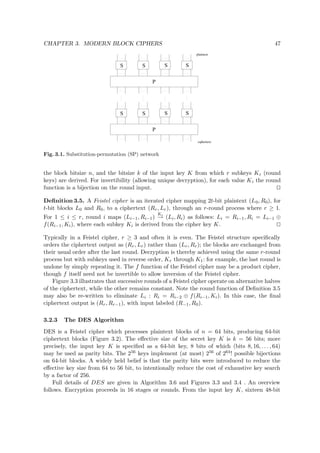
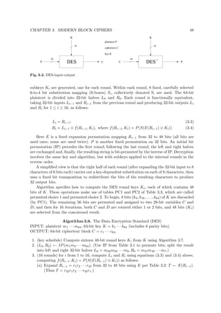
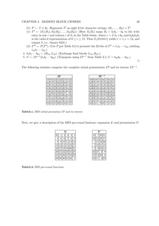
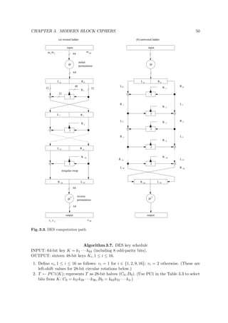
This document is an introduction to cryptography for graduate students. It covers the history and significance of cryptography, from its origins in ancient Egypt to its modern applications securing digital communications and electronic commerce. Key developments include the Data Encryption Standard (DES) in the 1970s, public-key cryptography introduced by Diffie and Hellman in 1976, and the RSA encryption algorithm published in 1978. The document provides an overview of simple and modern cryptosystems as well as cryptanalysis techniques. It also discusses cryptographic algorithms and protocols like RSA that are based on mathematical problems believed to be computationally difficult.

1. preliminary
Paper Script
Information Systems Security
157.738
MSc CompSci Sebastian Link
Version March 24, 2003
Massey University
Department of Information Systems
Private Bag 11222
Palmerston North
New Zealand

2. Plagiarism 2003
Since most of your marks will contribute towards your overall marks for the course we cannot
accept work which has been written jointly with others unless it is an approved group activity.
Similarly, if you include in your assignments material gained from other works in your sub-
ject area it is absolutely imperative that you give due acknowledgment. Deliberately copying
from printed work and passing it off as your own is cheating.
Copyright 2003
Books, journals, computer software and other teaching materials made available by Massey
University are for the student’s own studies and copying or use of them for other purposes is
an infringement of copyright.

3. 3
Preface
This lecture manual is intended to serve as an introduction to cryptography for graduate
Information Systems students. It is self-contained, especially fundamental mathematical con-
cepts are introduced in a way they will be needed to understand formally how and why
particular cryptographic methods work. Therefore, students are not required to have a deep
mathematical background. Unfortunately, proofs for theorems have been omitted in general,
although the author tried to convey as much mathematical flavour as possible.
The script covers a lot more than can be taught within a five day block course, where it is
important that lectures and exercises alternate.
Basically, greater extracts have been taken and adopted from Stinson’s “Cryptography: The-
ory and Practice” and from the “Handbook of Applied Cryptography”.
I am grateful for any kind of helpful suggestions and corrections.

4. Table of Contents
1 The Significance of Cryptography 1
1.1 Introduction . . . . . . . . . . . . . . . . . . . . . . . . . . . . . . . . . . . . . 1
1.2 Information Security and Cryptography . . . . . . . . . . . . . . . . . . . . . 2
2 Simple Cryptosystems 6
2.1 Basics on Functions . . . . . . . . . . . . . . . . . . . . . . . . . . . . . . . . 6
2.2 General Definitions . . . . . . . . . . . . . . . . . . . . . . . . . . . . . . . . . 8
2.3 Monoalphabetic Cryptosystems . . . . . . . . . . . . . . . . . . . . . . . . . . 10
2.3.1 Modular Arithmetic - Part I . . . . . . . . . . . . . . . . . . . . . . . . 11
2.3.2 The Shift Cipher . . . . . . . . . . . . . . . . . . . . . . . . . . . . . . 13
2.3.3 Permutations . . . . . . . . . . . . . . . . . . . . . . . . . . . . . . . . 15
2.3.4 The Substitution Cipher . . . . . . . . . . . . . . . . . . . . . . . . . . 16
2.3.5 Modular Arithmetic - Part II . . . . . . . . . . . . . . . . . . . . . . . 17
2.3.6 The Affine Cipher . . . . . . . . . . . . . . . . . . . . . . . . . . . . . 20
2.4 Polyalphabetic Cryptosystems . . . . . . . . . . . . . . . . . . . . . . . . . . . 24
2.4.1 The Vigenere Cipher . . . . . . . . . . . . . . . . . . . . . . . . . . . . 24
2.4.2 Matrices and determinants . . . . . . . . . . . . . . . . . . . . . . . . 26
2.4.3 The Hill Cipher . . . . . . . . . . . . . . . . . . . . . . . . . . . . . . . 30
2.4.4 The Permutation Cipher . . . . . . . . . . . . . . . . . . . . . . . . . . 32
2.5 Cryptanalysis . . . . . . . . . . . . . . . . . . . . . . . . . . . . . . . . . . . . 34
2.5.1 Different Levels of Attack . . . . . . . . . . . . . . . . . . . . . . . . . 34
2.5.2 Cryptanalysis of the Affine Cipher . . . . . . . . . . . . . . . . . . . . 35
2.5.3 Cryptanalysis of the Substitution Cipher . . . . . . . . . . . . . . . . . 37
2.5.4 Cryptanalysis of the Vigenere Cipher . . . . . . . . . . . . . . . . . . . 39
2.5.5 A known Plaintext Attack on the Hill Cipher . . . . . . . . . . . . . . 44
3 Modern Block Ciphers 45
3.1 Introduction to block ciphers . . . . . . . . . . . . . . . . . . . . . . . . . . . 45
3.2 DES . . . . . . . . . . . . . . . . . . . . . . . . . . . . . . . . . . . . . . . . . 46
3.2.1 Introduction . . . . . . . . . . . . . . . . . . . . . . . . . . . . . . . . 46
3.2.2 Product ciphers and Feistel ciphers . . . . . . . . . . . . . . . . . . . . 46
3.2.3 The DES Algorithm . . . . . . . . . . . . . . . . . . . . . . . . . . . . 47
3.2.4 Triple DES . . . . . . . . . . . . . . . . . . . . . . . . . . . . . . . . . 53
3.2.5 Security and Attacks on DES and Triple DES . . . . . . . . . . . . . . 54
3.2.6 DES Modes of Operation . . . . . . . . . . . . . . . . . . . . . . . . . 55
3.3 FEAL . . . . . . . . . . . . . . . . . . . . . . . . . . . . . . . . . . . . . . . . 56

5. ii
3.4 IDEA . . . . . . . . . . . . . . . . . . . . . . . . . . . . . . . . . . . . . . . . 58
3.5 SAFER . . . . . . . . . . . . . . . . . . . . . . . . . . . . . . . . . . . . . . . 61
3.6 RC5 . . . . . . . . . . . . . . . . . . . . . . . . . . . . . . . . . . . . . . . . . 64
3.7 The Advanced Encryption Standard: Rijndael . . . . . . . . . . . . . . . . . . 65
3.7.1 The Basic Algorithm . . . . . . . . . . . . . . . . . . . . . . . . . . . . 66
3.7.2 The Layers . . . . . . . . . . . . . . . . . . . . . . . . . . . . . . . . . 67
3.7.3 Decryption . . . . . . . . . . . . . . . . . . . . . . . . . . . . . . . . . 70
3.7.4 Design Considerations . . . . . . . . . . . . . . . . . . . . . . . . . . . 72
4 The RSA System 73
4.1 Introduction to public-key cryptography . . . . . . . . . . . . . . . . . . . . . 73
4.2 More mathematical background . . . . . . . . . . . . . . . . . . . . . . . . . . 77
4.2.1 Asymptotic notation . . . . . . . . . . . . . . . . . . . . . . . . . . . . 77
4.2.2 The Euclidean Algorithm and its extension . . . . . . . . . . . . . . . 78
4.2.3 Algorithms in
n . . . . . . . . . . . . . . . . . . . . . . . . . . . . . . 79
4.2.4 The Chinese Remainder Theorem and the Gauss-Algorithm . . . . . . 81
4.2.5 Some facts about groups . . . . . . . . . . . . . . . . . . . . . . . . . . 83
4.3 The RSA Cryptosystem . . . . . . . . . . . . . . . . . . . . . . . . . . . . . . 85
4.4 Probabilistic Primality Tests . . . . . . . . . . . . . . . . . . . . . . . . . . . 87
4.4.1 Fermat’s test . . . . . . . . . . . . . . . . . . . . . . . . . . . . . . . . 88
4.4.2 The Legendre and Jacobi symbols . . . . . . . . . . . . . . . . . . . . 89
4.4.3 Solovay-Strassen Test . . . . . . . . . . . . . . . . . . . . . . . . . . . 92
4.4.4 Miller-Rabin Test . . . . . . . . . . . . . . . . . . . . . . . . . . . . . . 93
4.4.5 A Comparison . . . . . . . . . . . . . . . . . . . . . . . . . . . . . . . 95
4.5 The Integer Factorization Problem . . . . . . . . . . . . . . . . . . . . . . . . 96
4.5.1 Trial Division . . . . . . . . . . . . . . . . . . . . . . . . . . . . . . . . 97
4.5.2 Pollard’s ρ-method . . . . . . . . . . . . . . . . . . . . . . . . . . . . . 97
4.5.3 Pollard’s p − 1-method . . . . . . . . . . . . . . . . . . . . . . . . . . . 99
4.5.4 Elliptic curve factoring . . . . . . . . . . . . . . . . . . . . . . . . . . . 101
4.5.5 Quadratic sieve factoring . . . . . . . . . . . . . . . . . . . . . . . . . 101
4.6 Attacks on RSA . . . . . . . . . . . . . . . . . . . . . . . . . . . . . . . . . . 103
4.6.1 Relation to factoring . . . . . . . . . . . . . . . . . . . . . . . . . . . . 103
4.6.2 Small Encryption Exponent b . . . . . . . . . . . . . . . . . . . . . . . 104
4.6.3 Forward Search Attack . . . . . . . . . . . . . . . . . . . . . . . . . . . 105
4.6.4 Small Decryption Exponent a . . . . . . . . . . . . . . . . . . . . . . . 105
4.6.5 Multiplicative Properties . . . . . . . . . . . . . . . . . . . . . . . . . 106
4.6.6 Common modulus attack . . . . . . . . . . . . . . . . . . . . . . . . . 106
4.6.7 Cycling attacks . . . . . . . . . . . . . . . . . . . . . . . . . . . . . . . 107
4.6.8 Message Concealing . . . . . . . . . . . . . . . . . . . . . . . . . . . . 107
4.7 RSA Encryption in Practice . . . . . . . . . . . . . . . . . . . . . . . . . . . . 108
5 The ElGamal Cryptosystem 110
5.1 The ElGamal Cryptosystem and Discrete Logarithms . . . . . . . . . . . . . 110
5.2 Algorithms for the Discrete Log Problem . . . . . . . . . . . . . . . . . . . . 113
5.2.1 The Baby-Step-Giant-Step Algorithm . . . . . . . . . . . . . . . . . . 113
5.2.2 Pollard’s ρ-algorithm for Discrete Logs . . . . . . . . . . . . . . . . . . 114
5.2.3 The Pohlig-Hellman Algorithm . . . . . . . . . . . . . . . . . . . . . . 116

6. iii
5.2.4 The Index Calculus Method . . . . . . . . . . . . . . . . . . . . . . . . 118
A Cryptography Timeline 121

7. Chapter 1
The Significance of Cryptography
1.1 Introduction
Cryptography has a long and fascinating history. The most complete non-technical account of
the subject is Kahn’s The Codebreakers. This book traces cryptography from its initial use by
the Egyptians some 4000 years ago, to the twenties century where it played a crucial role in
the outcome of both world wars. Completed in 1963, Kahn’s book covers those aspects of the
history which are most significant (up to that time) to the development of that subject. The
predominant practitioniers of the art were associated with the military, the diplomatic service
and government in general. Cryptography was used as a tool to protect national secrets and
strategies.
The proliferation of computers and communications systems in the 1960s brought with
it a demand from the private sector for means to protect information in digital form and to
provide security services. Beginning with the work of Feistel at IBM in the early 1970s and
culminating in 1977 with the adoption as a U.S. Federal Information Processing Standard
for encrypting unclassified information, DES, the Data Encryption Standard, is the most
well-known cryptographic mechanism in history. It remains the standard means for securing
electronic commerce for many financial institutions around the world.
The most striking development in the history of cryptography came 1976 when Diffie and
Hellman published New Directions in Cryptography. This paper introduced the revolutionary
concept of public-key cryptography and also provided a new and ingenious method for key
exchange, the security of which is based on the intractibility of the discrete logarithm problem.
Although the authors had no practical realization scheme at the time, the idea was clear
and it generated extensive interest and activity in the cryptographic community. In 1978
Rivest, Shamir and Adleman discovered the first practical public-key encryption and signature
scheme, now referred to as RSA. The RSA scheme is based on another hard mathematical
problem, the intractibility of factoring large integers. This application of a hard mathematical
problem to cryptography revitalized efforts to find more efficent methods to factor. The 1980s
saw major advances in this area but none which rendered the RSA system insecure. Another
class of powerful and practical public-key schemes was found by ElGamal in 1985. These are
also based on the discrete logarithm problem.
One of the most significant contributions provided by public-key cryptography is the digital
signature. In 1991 the first international standard for digital signatures (ISO/IEC 9797) was
adopted. It is based on the RSA public-key scheme. In 1994 the U.S. Government adopted

8. CHAPTER 1. THE SIGNIFICANCE OF CRYPTOGRAPHY 2
the Digital Signature Standard, a mechanism based on the ElGamal public-key scheme.
The search for new-public schemes, improvements to existing cryptographic mechanisms,
and proof of security continues at a rapid pace. Various standards and infrastructures involving
cryptography are being put in place. Security products are being developed to address the
security needs of an information intensive society.
The purpose of this paper is to give an up-to-date treatise of the principles, techniques,
and algorithms of interest in cryptographic practice. Emphasis has been placed on those
aspects which are most practical and applied. The reader will be aware of the basic issues and
encouraged to further studies in the fields of interest. Due to time restrictions and in view of
the practical intention of this paper, most results will be stated without proofs.
1.2 Information Security and Cryptography
The concept of information will be taken to be an understood quantity. To introduce cryp-
tography, an understanding of issues related to information security in general is necessary.
Information security manifests itself in many ways according to the situation and requirement.
Regardless of who is involved, to one degree or another, all parties to a transaction must have
confidence that certain objectives associated with information security have been met. Some
of these objectives are listed in Table 1.1.
privacy keeping information secret from all but those who
or confidentiality are authorized to see it
data integrity ensuring information has not been altered by unauthorized
or unknown means
entity authentication corroboration of the identity of an entity (e.g., a person,
or identification a computer terminal, a credit card, etc.)
message corroborating the source of information; also known as data
authentication origin authentication
signature a means to bind information to an entity
authorization conveyance, to another entity, of official sanction to do or be something
validation a means to provide timeliness of authorization to use or manipulate
information or resources
access control restricting access to resources to privileged entities
certification endorsement of information by a trusted entity
timestamping recording the time of creation or existence of information
witnessing verifying the creation or existence of information by an
entity other than the creator
receipt acknowledgement that information has been received
confirmation acknowledgement that services have been provided
ownership a means to provide an entity with the legal right to use or
transfer a resource to others
anonymity concealing the identity of an entity involved in some process
non-repudiation preventing the denial of previous commitments or actions
revocation retraction of certification or authorization
Table1.1. Some information security objectives

9. CHAPTER 1. THE SIGNIFICANCE OF CRYPTOGRAPHY 3
Over the centuries, an elaborate set of protocols and mechanisms has been created to deal
with information security issues when the information is conveyed by physical documents.
Often the objectives of information security cannot solely be achieved through mathematical
algorithms and protocols alone, but require procedural techniques and abidance of laws to
achieve the desired result. For example, privacy of letters is provided by sealed envelopes
delivered by an accepted mail service. The physical security of the envelope is, for practical
necessity, limited and so laws are enacted which make it a criminal offense to open mail for
which one is not authorized. It is sometimes the case that security is achieved not through
the information itself but through the physical document recording it. For example, paper
currency requires special inks and material to prevent counterfeiting.
Conceptually, the way information is recorded has not changed dramatically over time.
Whereas information was typically stored and transmitted via telecommunications systems,
some wireless. What has changed dramatically is the ability to copy and alter information.
One can make thousands of identical copies of a piece of information stored electronically and
each is indistinguishable from the original. With information on paper, this is more difficult.
What is needed then for a society where information is mostly stored and transmitted in
electronic form is a means to ensure information security which is independent of the physical
medium recording or conveying it and such that the objectives of information security rely
solely on digital information itself.
One of the fundamental tools used in information security is the signature. It is a building
block for many other services such as non-repudiation, data origin authentication, identifica-
tion, and witnessing, to mention a few. Having learned the basics in writing, an individual is
taught how to produce a handwritten signature for the purpose of identification. At contract
age the signature evolves to take on a very integral part of the person’s identity. This signa-
ture is intended to be unique to the individual and serve as a means to identify, authorize,
and validate. With electronic information the concept of a signature needs to be redressed; it
cannot simply be something unique to the signer and independent of the information signed.
Electronic replication of it is so simple that appending a signature to a document not signed
by the originator of the signature is almost a triviality.
Analogues of the “paper protocols” currently in use are required. Hopefully these new
electronic based protocols are at least as good as those they replace. There is a unique oppor-
tunity to society to introduce new and more efficient ways of ensuring information security.
Much can be learned from the evolution of the paper based system, mimicking those aspects
which have served us well and removing the inefficiencies.
Achieving information security in an electronic society requires a vast array of techniques
and legal skills. There is, however, no guarantee that all of the information security objec-
tieves deemed necessary can be adequately met. The technical means is provided through
cryptography.
Definition 1.1. Cryptography is the study of mathematical techniques related to aspects of
information security such as confidentiality, data integrity, entity authentication, and data
origin authentication.
Cryptography is not the only means of providing information security but rather one set of
techniques.

10. CHAPTER 1. THE SIGNIFICANCE OF CRYPTOGRAPHY 4
Cryptographic goals
Of all the information security objectives listed in Table 1.1, the following four form a frame-
work upon which the others will be derived. (1) privacy or confidentiality; (2) data integrity;
(3) authentication; and (4) non-repudiation.
1. Confidentiality is a service used to keep the content of information from all but those
authorized to have it. Secrecy is a term synonymous with confidentialiy and privacy. There
are numerous approaches to providing confidentiality, ranging from physical protection to
mathematical algorithms which render data unintelligible.
2. Data integrity is a service which addresses the unauthorized alteration of data. To assure
data integrity, one must have the ability to detect data manipulation by unauthorized
parties. Data manipulation includes such things as insertion, deletion and substitution.
3. Authentication is a service related to identification. This function applies to both entities
and information itself. Two parties entering into a communication should identify each
other. Information delivered over a channel should be authenticated as to origin, date of
origin, data content, time sent, etc. For these reasons this aspect of cryptography is usually
subdivided into two major classes: entity authentication and data origin authentication.
Data origin authentication implicitly provides data integrity (for if a message is modified,
the source has changed).
4. Non-repudiation is a service which prevents an entity from denying previous commitments
or actions. When disputes arise due to an entity denying that certain actions were taken,
a means to resolve the situation is necessary. For example, one entity may authorize the
purchase of property by another entity and later deny such authorization was granted. A
procedure involving a trusted third party is needed to resolve the dispute.
A fundamental goal of cryptography is to adequately address these four areas in both theory
and practice. Cryptography is about the prevention and detection of cheating and other
malicious activities.
This paper is intended to describe a number of basic cryptographic tools (primitives) used
to provide information security. Unfortunately, we cannot cover all different branches that
employ primitives. Nevertheless, we provide a schematic listing of the primitives and how
they relate in Figure 1.1.
These primitives should be evaluated with respect to various criteria such as:
1. Level of Security. This is usually difficult to quantify. Often it is given in terms of the
number of operations required (using the best methods currently known) to defeat the
intended objective. Typically the level of security is defined by an upper bound on the
amount of work necessary to defeat the objective. This is sometimes called the work
factor.
2. Functionality. Primitives will need to be combined to meet various information security
objectives. Which primitives are most effective for a given objective will be determined
by the basic properties of the primitives.
3. Methods of operation. Primitives, when applied in various ways and with various inputs,
will typically exhibit different characteristics; thus one primitive could provide very dif-
ferent functionality depending on its mode of operation or usage.
4. Performance. This refers to the efficiency of a primitive in a particular mode of operation.
(For example, an encryption algorithm may be rated by the number of bits per second
which it can encrypt.)

11. CHAPTER 1. THE SIGNIFICANCE OF CRYPTOGRAPHY 5
Public−key
ciphers
Signatures
Identification
primitives
Security
Primitives Primitives
Symmetic−key
Unkeyed
Primitives
Primitives
Public−key
Block
Arbitrary length
hash function
One−way
permutation
Random sequences
Symmetric−key
ciphers
Arbitrary length
hash functions(MACS)
Signatures
Pseudorandom
sequences
Identification
primitives
ciphers
Stream
ciphers
Fig. 1.1. A taxonomy of cryptographic primitives
5. Ease of Implementation. This refers to the difficulty of realizing the primitive in a practical
instantation. This might include the complexity of implementing the primitive in either
a software or hardware environment.
The relative importance of various criteria is very much dependent on the application and
resources available. For example, in an environment where computing power is limited one
may have to trade off a very high level of security for better performance of the system as a
whole.
Cryptography, over the ages, has been an art practised by many who have devised ad
hoc techniques to meet some of the information security requirements. The last twenty years
have been a period transition as the discipline moved from an art to a science. There are now
several international scientific conferences devoted exclusively to cryptography and also an
international scientific organization, the International Association for Cryptologic Research
(IACR), aimed at fostering research in the area.

12. Chapter 2
Simple Cryptosystems
2.1 Basics on Functions
One concept which is absolutely fundamental to cryptography is that of a function in the
mathematical sense. A function is alternatively referred to as a mapping or a transformation.
A set consists of distinct objects which are called elements of the set. For example, a set
X might consist of the elements a, b, c, and is denoted X = {a, b, c}.
Definition 2.1. A function is defined by two sets X and Y and a rule f which assigns to
each element in X precisely one element in Y . The set X is called the domain of the function
and Y the codomain. If x is an element of X (usually written x ∈ X) the image of x is the
element in Y which the rule f associates with x; the image y of x is denoted by y = f(x).
Standard notation for a function f from set X to set Y is f : X → Y . If y ∈ Y , then a
preimage of y is an element x ∈ X for which f(x) = y. The set of all elements in Y which
have at least one preimage is called the image of f, denoted Im(f).
Example 2.1. Consider the sets X = {a, b, c}, Y = {1, 2, 3, 4}, and the rule f from X to Y
defined as f(a) = 2, f(b) = 4, f(c) = 1. Figure 2.1 shows a schematic of the sets X, Y and the
function f. The preimage of the element 2 is a. The image of f is {1, 2, 4}.
1
X
2
3
4
a
b
c
f
Y
Fig. 2.1. A function f from a set X of three elements to set Y of four elements
Thinking of a function in term of the schematic (sometimes called a functional diagram) given
in Figure 2.1, each element in the domain X has precisely one arrowed line originating from

13. CHAPTER 2. SIMPLE CRYPTOSYSTEMS 7
it. Each element in the codomain Y can have any number of arrowed lines incident to it
(including zero lines).
Often only the domain X and the rule f are given and the codomain is assumed to be the
image of f. This point is illustrated with two examples.
Example 2.2. Take X = {1, 2, 3, . . . , 10} and let f be the rule that for each x ∈ X, f(x) = rx,
where rx is the remainder when x2 is divided by 11. Explicitely then
f(1) = 1 f(2) = 4 f(3) = 9 f(4) = 5 f(5) = 3
f(6) = 3 f(7) = 5 f(8) = 9 f(9) = 4 f(10) = 1.
The image of f is the set Y = {1, 3, 4, 5, 9}.
Example 2.3. Take X = {1, 2, 3, . . . , 1050} and let f be the rule f(x) = rx, where rx is the
remainder when x2 is divided by 1050 + 1 for all x ∈ X. Here it is not feasible to write down
f explicitely as in Example 2.2, but nonetheless the function is completely specified by the
domain and the mathematical description of the rule f.
Definition 2.2. A function or transformation is 1 – 1 (one to one) iff each element in the
codomain Y is the image of at most one element in the domain X. We call such a function
sometimes injective.
Definition 2.3. A function or transformation is onto iff each element in the codomain Y is
the image of at least one element in the domain. Equivalently, a function f : X → Y is onto
iff Im(f) = Y . We sometimes call such a function surjective.
Definition 2.4. A function f : X → Y is called bijection if and only if it is 1 – 1 and
Im(f) = Y .
Proposition 2.5. If f : X → Y is 1 – 1 then f : X → Im(f) is a bijection. In particular,
if f : X → Y is 1 – 1 (onto), and X and Y are finite sets of the same size, then f is a
bijection.
In terms of the schematic representation, if f is a bijection, then each element in Y has exactly
one arrowed line incident with it. The functions described in Examples 2.1 and 2.2 are not
bijections. In Example 2.1 the element 3 is not the image of any element in the domain. In
Example 2.2 each element in the codomain has two preimages.
Definition 2.6. If f is a bijection from X to Y then it is a simple matter to define a bijection
g from Y to X as follows: for each y ∈ Y define g(y) = x where x ∈ X and f(x) = y. This
function g obtained from f is called the inverse function of f and is denoted by g = f −1.
Example 2.4. Let X = {a, b, c, d, e}, and Y = {1, 2, 3, 4, 5}, and consider the rule f given by
the arrowed edges in Figure 2.2. f is a bijection and its inverse g is formed simply by reversing
the arrows on the edges. The domain of g is Y and the codomain is X.
Note that if f is a bijection, then so is f−1. In cryptography bijections are used as the tool
for encrypting messages and the inverse transformations are used to decrypt. Notice that if
the transformations were not bijections then it would not be possible to always decrypt to a
unique message.

14. CHAPTER 2. SIMPLE CRYPTOSYSTEMS 8
f
X Y
a
b
c
d
e
1
2
3
4
5
XY
a
b
c
d
e
1
2
3
4
5
g
Fig. 2.2. A bijection f and its inverse g = f−1
Exercise 2.7. 1. Consider the function f : → with x → 2x ∈ . What kind of
function is f in terms of onto, 1–to–1 and bijection? What happens, if we change the
codomain of this f to 2 = {0, 2, 4, 6, 8, . . .}?
2. Why is the function g :
→ with
x →
2x , if x ≥ 0
3|x| , if x < 0
1–to–1, but not onto? How
can the codomain be changed to make g a bijection?
3. What can be said about the functions h1, h2 :
→ with h1(x) =
2x , if x ≥ 0
2|x| + 1 , if x < 0
and h2(x) =
2x , if x ≥ 0
2|x| − 1 , if x < 0
?
2.2 General Definitions
The scientific study of any discipline must be built upon rigorous definitions arising from
fundamental concepts. What follows is a list of terms and basic concepts used throughout
this paper.
We begin with the very fundamental concept of a cryptosystem which decribes in a formal
way the main goal of cryptography.
Definition 2.8. A cryptosystem is a five-tupel (P, C, K, E, D), where the following conditions
are satisfied
1. P is a finite set of possible plaintexts
2. C is a finite set of possible ciphertexts
3. K, the keyspace, is a finite set of possible keys
4. For each K ∈ K, there is an encryption rule eK ∈ E and a corresponding decryption rule
dK ∈ D. Each eK : P → C and dK : C → P are functions such that dK(eK(x)) = x for
every plaintext x ∈ P.
Since this definition uses very mathematical notation we explain what the certain components
of a cryptosystem should mean. Therefore we consider the following figure which gives a
schema of a two-party communication using enryption.
Note 2.9. Referring to Figure 2.3, we can now informally say what the objective of cryp-
tography should be. Two people, usually referred to as Alice and Bob, want to communicate
over an insecure channel in such a way that an opponent, Oscar, cannot understand what

15. CHAPTER 2. SIMPLE CRYPTOSYSTEMS 9
Alice
unsecure channel
Adversary
c
m
destination
decryption
Bob
k
d (c)=m
encryption
plaintext
source
m
e (m)=c
k
Fig. 2.3. Two-party communication
is being said. This channel could be a telephone line or a computer network, for example.
The information that Alice wants to sent to Bob, which we call plaintext message m, can be
English text, numerical data, computer code or anything at all – its structure is completely
arbitrary. Alice encrypts the plaintext, using a predetermined key K ∈ K, and sends the
resulting ciphertext eK(m) over the channel. Oscar, upon seeing the ciphertext in the channel
by eavesdropping, cannot determine what the plaintext m was; but Bob, who knows the en-
cryption key K, can decrypt the ciphertext using the corresponding decryption rule dK and
reconstruct the plaintext by dK(eK(m)) = m.
The main property of Definition 2.8 is property 4. It says that if a plaintext m is enrypted
using eK, and the resulting ciphertext is subsequently decrypted using dK, then the original
plaintext m results.
Note 2.10. Clearly, it must be the case that each encryption function eK is an injective
function, i.e. for all messages m1, m2 ∈ P which satisfy eK(m1) = eK(m2) we have m1 = m2
or equivalentely, from m1 = m2 we derive eK(m1) = eK(m2). Otherwise, decryption could
not be accomplished in an unambigous manner. For example, if
y = eK(m1) = eK(m2)
where m1 = m2, then Bob has no way of knowing whether y should decrypt to m1 or m2.
Cryptographic techniques are typically divided into two generic types: symmetric-key and
public-key. First we now turn to the symmetric-key methods and treat the other ones in
chapter 4 and 5.

16. CHAPTER 2. SIMPLE CRYPTOSYSTEMS 10
2.3 Monoalphabetic Cryptosystems
We begin with spelling out what should be understood under a symmetric-key encryption.
Definition 2.11. A cryptosystem (P, C, K, E, D) is said to be symmetric-key if for each asso-
ciated enryption/decryption rule pair (eK, dK), it is computationally easy1 to determine dK
knowing only eK, and to determine eK from dK.
According to this definition, the term symmetric-key becomes appropriate. A two-party com-
munication using symmetric-key encryption can be described by the block diagram of Figure
2.4, which is Figure 2.3 with the addition of the secure channel, meaning no adversary has
access to it. One of the major issues with symmetric-key systems is to find an efficient method
to agree upon and exchange keys securely. The problem is referred to as the key distribution
problem.
d
k
e
k
Adversary
secure channel
Alice
unsecure channel
cencryption
plaintext
source
m
key
source
m
destination
decryption
d (c)=m
Bob
k
e (m)=c
k
Fig. 2.4. Two-party communication using encryption, with a secure channel for key exchange. The
descryption rule dK can be efficently computed from the encryption rule eK.
It is assumed that all parties know the set of encryption/decryption rules, the only information
which should be kept secret is the decryption rule dK. However, in symmetric-key encryption,
this means that the encryption rule eK must also be kept secret, as dK can be deduced from
1
this means usually, there is a polynomial algorithm with input eK (dK) and output dK (ek)

17. CHAPTER 2. SIMPLE CRYPTOSYSTEMS 11
eK. In Figure 2.4 the encryption rule eK is transported from one entity to the other with the
understanding that both can construct the decryption rule dK.
In addition, we can divide the class of symmetric-key cryptosystems into monoalphabetic
ones and polyalphabetic ones.
Definition 2.12. A cryptosystem is called monoalphabetic iff, once a key is chosen, each
alphabetic character is mapped to a unique alphabetic character. Accordingly, a cryptosystem
is called polyalphabetic iff there are more than only one possible characters that an alphabetic
character can be mapped to.
We would like to investigate certain examples for such cryptosystems. Therefore we will start
with the monoalphabetic ones and will see that these cryptosystems are not secure in some
manner. We will come later on to the other class and will realize that these ones are a bit
securer, but there will still be quite simple tools to break them.
Before we can finally start with examples we have to lay some foundations concerning the
mathematical background for these.
2.3.1 Modular Arithmetic - Part I
The first problem that arises in accordance to Definition 2.8 is the finite nature of objects
within a cryptosystem. In fact, that is no real problem, but we have to find mathematical
models that help us to deal with them. We used to be acquainted with the infinte set of
nonegative integers, the natural numbers = {0, 1, 2, . . .}, and the operations of addition
and multiplication on it. Now we are concerned with certain subsets of and have to define
a new addition and a new multiplication on it.
Definition 2.13. Suppose we are given two integers a, b ∈
and a positive integer m ∈
{0}. Then we write a ≡ b (mod m) iff m divides b − a. The phrase a ≡ b (mod m) is read
as “a is congruent to b modulo m”. The integer is called the modulus.
We can give a characterization of the fact, that two integers a and b are congruent modulo
an integer m.
Note 2.14. Suppose we divide a and b by m, obtaining integer quotients and remainders in
the following way:
a = q1m + r1 with 0 ≤ r1 ≤ m − 1
and
b = q2m + r2 with 0 ≤ r2 ≤ m − 1 .
Then it is not difficult to see that a ≡ b (mod m) holds if and only if r1 = r2 holds. This means
that two integer are congruent modulo a certain modulus iff the division of these integers by
that certain modulus gives the same remainder.
In addition to the last fact, we can list a few more.
Proposition 2.15. For all a, a1, b, b1, c ∈
, the following are true.
1. (reflexivity) a ≡ a (mod n)
2. (symmetry) If a ≡ b (mod n) then b ≡ a (mod n).

18. CHAPTER 2. SIMPLE CRYPTOSYSTEMS 12
3. (transitivity) If a ≡ b (mod n) and b ≡ c (mod n), then a ≡ c (mod n).
4. If a ≡ a1 (mod n) and b ≡ b1 (mod n), then a + b ≡ a1 + b1 (mod n) and ab ≡ a1b1
(mod n).
With this background we are now able to define our object of interest, namely the ring of
integers modulo a certain modulus.
Definition 2.16. Let m be a positive integer. The ring of integers modulo m is defined as
the set
m := {0, 1, . . . , m − 1} together with a mapping +m :
m ×
m →
m which sends
m ×
m (a, b) → a+b (mod m), where + denotes the usual addition on
, and a mapping
∗m :
m ×
m →
m which sends
m ×
m (a, b) → a · b (mod m), where · is the ordinary
multiplication on
.
Addition and multiplication in
m work exactely like real addition and multiplication, except
that the results are reduced modulo m. Therefore we write instead of +m and ∗m rather +
and ∗, respectively, we even omit as usual the product symbol ∗.
Example 2.5. Let m = 7, i.e. we have
7 = {0, 1, 2, 3, 4, 5, 6}. Suppose, we would like to
compute 3 + 5 in
7. As integers, we have 3 + 5 = 8. To reduce 8 modulo 7 we receive
8 = 1 · 7 + 1, so 8 mod 7 = 1, and hence 3+5=1 in
7.
Computing 11∗13 within
14 means to compute 11∗13 = 143 as integers, to reduce 143 mod
14, i.e. we perform ordinary long division: 143 = 10 · 14 + 3, so 143 mod 14 = 3, and hence
11 ∗ 13 = 3 within
14.
We called the triple (
m, +, ·) a ring, which is in fact, a certain algebraic structure that satisfies
a couple of nice properties. Strictly speaking, we would have to proof these properties, but
we are content to list them.
Proposition 2.17. The ring (
m, +, ·) is well-definied and commutative, i.e.
1. addition is closed, i.e., for any a, b ∈
m we have a + b ∈
m
2. addition is commutative, i.e., for any a, b ∈
m we have a + b = b + a
3. addition is associative, i.e., for any a, b, c ∈
m we have (a + b) + c = a + (b + c)
4. 0 is an additive identity, i.e., for any a ∈
m we have a + 0 = a = 0 + a
5. the additive inverse of any a ∈
m is m − a, i.e., a + (m − a) = 0 = (m − a) + a for any
a ∈
m
6. multiplication is closed, i.e., for any a, b ∈
m we have ab ∈
m
7. multiplication is commutative, i.e., for any a, b ∈
m we have ab = ba
8. multiplication is associative, i.e., for any a, b, c ∈
m we have a(bc) = (ab)c
9. 1 is a multiplicative identity, i.e., for any a ∈
m we have a · 1 = a = 1 · a
10. multiplication distributes over addition, i.e., for any a, b, c ∈
m we have (a + b)c =
(ac) + (bc) and a(b + c) = ab + ac
We conclude this short introduction to elementary arithmetic with a remark on certain alge-
braic objects.
Note 2.18. (
m, +) forms an algebraic structure called a group according to the properties
1,3,4,5. This group is even abelian due to property 2.

19. CHAPTER 2. SIMPLE CRYPTOSYSTEMS 13
(
m, ∗) forms an algebraic structure called monoid according to the properties 6,8 and 9,
that is even commutative due to property 7.
Property 10 guarantees that both mappings are amicable, such that (
m, +, ∗) indeed
becomes a ring.
Notice, that there are in general no multiplicative inverses for elements in
m, i.e., a is
called a multiplicative inverse of a iff aa = 1 = a a holds. A commutative ring, in which every
element except the zero element 0 has a multiplicative inverse, is called a field.
Exercise 2.19. 1. Set up tables for (
6, +6, 0) and (
6, ∗6, 1) to make statements about its
algebraic structures. What about (
6, +6, ∗6, 0, 1)?
2. Do the same for (
7, +7, ∗7, 0, 1).
2.3.2 The Shift Cipher
We can now turn to the first example of a cryptosystem which is, in fact, the simpliest to
consider. We would use the Shift Cipher with a modulus of 26 to encrypt ordinary English
text by setting up a correspondence between alphabetic characters and numbers between 0
and 25 as follows: A ↔ 0, B ↔ 1, . . . , Z ↔ 25. Since we will use this bijection in several
examples, let’s record it for future use.
A B C D E F G H I J K L M
0 1 2 3 4 5 6 7 8 9 10 11 12
N O P Q R S T U V W X Y Z
13 14 15 16 17 18 19 20 21 22 23 24 25
We will now describe the Shift Cipher by definition of its cryptosystem.
Definition 2.20. Let P = C = K =
26. For 0 ≤ K ≤ 25, define
eK(x) = x + K mod 26
and
dK(y) = y − K mod 26
for x, y ∈
26.
In order to get an impression how the enryption works, we give a simple example. By the
way, we are going to use upper case letters for ciphertext and lower case letters for plaintext,
in order to improve readability.
Example 2.6. Let the key for a Shift Cipher be K = 13. and the plaintext is
keyliesbelowcarpet.
We first convert the plaintext to a sequence of integers using the specified correspondence,
obtaining the following.
10 4 24 11 8 4 18 1 4 11 14 22 2 0 17 15 4 19
Next, we add 13 to each value, reducing each sum modulo 26.

20. CHAPTER 2. SIMPLE CRYPTOSYSTEMS 14
23 17 11 24 21 17 5 14 17 24 1 9 15 13 4 2 21 6
Finally, we convert the sequence of integers to alphabetic characters, obtaining the ciphertext
XRLYVRFORYBJPNECVG.
To decrypt the ciphertext, Bob will first convert the ciphertext to a sequence of integers, then
subtract 13 from each value reducing modulo 26, and finally convert the sequence of integers
to alphabetic characters.
If a cryptosystem is to be of practical use, it should satisfy certain properties. We informally
enumerate two of these properties now.
1. Each encryption function eK and each decryption function dK should be efficiently com-
putable.
2. An opponent, upon seeing a ciphertext string y, should be unable to determine the key
K that was used, or the plaintext string x.
The second property is defining, in a very vague way, the idea of “security”. The process of
attempting to compute the key K, given a string of ciphertext y, is called cryptanalysis. Note
that, if Oscar can determine K, then he can decrypt y just as Bob would, using dK. Hence,
determining K is at least as difficult as determining the plaintext string x.
We observe that the Shift Cipher (modulo 26) is not secure, since it can be cryptanalyzed
by the obvious method of exhaustive key search. Since there are only 26 possible keys, it
is easy to try every possible decryption rule dK until a ”’meaningful”’ plaintext string is
obtained. This is illustrated in the following example.
Example 2.7. Given the ciphertext string
YMNXNXYMJTSJDTZFWJQTTPNSLKTW,
we successively try the decryption rules d0, d1, etc. The following is obtained.
ymnxnxymjtsjdtzfwjqttpnslktw
xlmwmwxlisricsyevipssomrkjsv
wklvlvwkhrqhbrxduhorrnlqjiru
vjkukuvjgqpgaqwctgnqqmkpihqt
uijtjtuifpofzpvbsfmppljohgps
thisistheoneyouarelookingfor
At this point, we have determined the plaintext and we can stop. The key is K = 5.
On average, a plaintext will be computed after trying 26/2=13 decryption rules.
As the above example indicates, a necessary condition for a cryptosystem to be secure is
that an exhaustive key search should be infeasible, i.e., the keyspace should be very large. As
might be expected, a large keyspace is not sufficent to guarantee security.
Exercise 2.21. 1. Proof that the Shift Cipher is correct in the sense that dK(eK(x)) = x
for x ∈
26.
2. Encrypt the following text with a shift cipher using K = 17:

21. CHAPTER 2. SIMPLE CRYPTOSYSTEMS 15
“New Zealand never lost to Scotland and no one expected that record to end at
Murrayfield.”
3. Decrypt the following text that has been encrypted with a Shift Cipher using K = 23:
“QEBXIIYIXZHPTBOBYVZLJJLKZLKPBKQPELOQMOFZBACXSLRO
FQBPQLTFKKLQGRPQQEFPJXQZEYRQQEBZRMCFKXIXPTBII.”
4. Decrypt the following text having been encrypted using a Shift Cipher:
“XLSYKLXLIEPPFPEGOWASRLERHWSQIPCIRSYKLVIEP
MXMIWHSRSXEPAECWQMVVSVXLIIBTIGXEXMSRW.”
2.3.3 Permutations
Permutations are functions which are often used in various cryptographic constructs, for
example in the next paragraph.
Definition 2.22. Let S be a finite set of elements. A permutation p on S is a bijection
(Definition 2.4) from S to itself, i.e., p : S → S.
Example 2.8. Let S = {1, 2, 3, 4, 5}. A permutation p : S → S is defined as follows:
p(1) = 3, p(2) = 5, p(3) = 4, p(4) = 2, p(5) = 1 .
A permutation can be described in varios ways. It can be displayed as above or as an array:
p =
1 2 3 4 5
3 5 4 2 1
(2.1)
where the top row in the array is the domain and the bottom row is the image under the
mapping p. Of course, other representations are possible.
Since permutations are bijections, they have inverses. If a permutation is written as an array
see (2.1), its inverse is easily found by interchanging the rows in the array and reordering
the elements in the new top row if desired (the bottom row would have to be reordered
correspondingly). The inverse of p in Example 2.8 is
p−1
=
1 2 3 4 5
5 4 1 3 2
.
Example 2.9. Let X be the set of integers {0, 1, 2, . . . , pq−1} where p and q are distinct large
primes (for example, p and q are each about 100 decimal digits long), and suppose neither
p−1 and q −1 is divisible by 3. Then the function p(x) = rx, where rx is the remainder when
x3 is divided by pq, can be shown to be a permutation. Determining the inverse permutation
is computationally infeasible by today’s standard unless p and q are known.
Exercise 2.23. 1. Find the inverses for the following permutations p and q:
p(1)=2, p(2)=3, p(3)=5, p(4)=1, p(5)=6, p(6)=4
q(1)=3, q(2)=4, q(3)=5, q(4)=6, q(5)=7, q(6)=1, q(7)=2.

22. CHAPTER 2. SIMPLE CRYPTOSYSTEMS 16
2. Let Sn be the set of all permutations of {1, . . . , n}. Define on Sn an operation · as follows:
for
1 2 · · · n
x1 x2 · · · xn
,
1 2 · · · n
y1 y2 · · · yn
∈ Sn define
1 2 · · · n
x1 x2 · · · xn
·
1 2 · · · n
y1 y2 · · · yn
=
1 2 · · · n
yx1 yx2 · · · yxn
.
Set up a table for (S3, ·). What kind of structure is it?
2.3.4 The Substitution Cipher
Another well-known cryptosystem is the Substitution Cipher. This cryptosystem has been
used for hundreds of years. Puzzle “cryptograms” in newspapers are examples of Substitution
Ciphers, which is defined as follows.
Definition 2.24. Let P = C =
26. K consists of all possible permutations of the 26 symbols
0, 1, . . . , 25. For each permutation K π :
26 →
26, define
eπ(x) = π(x) ,
and
dπ(y) = π−1
(y) ,
where π−1 is the inverse permutation to π.
Actually, in the case of the Substitution Cipher, we might as well take P and C both to
be the 26-letter English alphabet. We used
26 in the Shift Cipher because encryption and
decryption were algebraic operations. But in the Substitution Cipher, it is more convinient
to think of encryption and decryption as permutations of algebraic characters.
Here is an example of a “random” permutation, π, which could comprise an encryption
function.
Example 2.10. We use our representation with an array and define π to be
a b c d e f g h i j k l m n o p q r s t u v w x y z
X N Y A H P O G Z Q W B TS F L R C V M U E K J D I
.
Thus, eπ(a) = X, eπ(b) = N, etc. The decryption function is the inverse permutation. This is
formed by writing the second line first, and then sorting in alphabetic order. The following is
obtained for π−1
A B C D E F G H I J K L M N O P Q R S T U V W X Y Z
d l r y v o h e z x w p tb g f j q n m u s k a c i
.
Hence, dπ(A) = d, dπ(B) = l, etc.
Given the ciphertext
MGZVYZLGHCMHJMYXSSFMNHAHYCDLMHA
we immediately obtain the plaintext
thisciphertextcannotbedecrypted .

23. CHAPTER 2. SIMPLE CRYPTOSYSTEMS 17
We make one final note concerning the possibilities of breaking the Substitution Cipher.
Note 2.25. A key for the Substitution Cipher just consists of a permutation of the 26 alpha-
betic characters. The number of these permutations is 26!, which is more than 4.0 × 1026, a
very large number. Thus, an exhaustive key search is infeasible, even for a computer. Never-
theless, there are other methods for cryptoanalysing the Substitution Cipher.
Exercise 2.26. 1. Suppose you are given the key
a b c d e f g h i j k l m n o p q r s t u v w x y z
Q D J H N Y B V L T X F P R G A S M W E Y I C O K U
.
Encrypt the following message using a Substitution Cipher:
“He walks on, does not look back, he pretends he cannot hear her, starts to whistle as
he crosses the street, seems embarrassed to be there.”
2. Now, suppose you are given the key
a b c d e f g h i j k l m n o p q r s t u v w x y z
B A D C F E H G J I L K N M P O R Q T S V U X W Z Y
.
Decrypt the following message having been encrypted with a Substitution Cipher and the
key above:
“ZPVDBMSFKKEQPNSGFKJMFTPEGFQEBDFZPVDBMT
FFSGBSTGFGBTAFFMSGFQFOQPABAKZAFFMNPUFC
PMEQPNFUFQZOKBDFDPTTGFCJCMPSEJSJMSGFQF.”
2.3.5 Modular Arithmetic - Part II
We have to lay some more foundations in order to be able to continue our examples for
cryptosystems. Therefore, we first want to introduce the idea of greatest common divisors
before we go further with modular arithmetic.
We have already made use of the idea of divisibility, but we now would like to define
precisely this concept.
Definition 2.27. Let a, b ∈
be integers. Then a divides b (equivalently: a is a divisor of
b, or a is a factor of b) iff there is an integer c such that b = ac. If a divides b, then this is
denoted by a|b.
The following are some elementary properties of divisibility.
Proposition 2.28. For all a, b, c ∈
, the following are true:
1. a|a.
2. If a|b and b|c, then a|c.
3. If a|b and a|c, then a|(bx + cy) for all x, y ∈
.

24. CHAPTER 2. SIMPLE CRYPTOSYSTEMS 18
4. If a|b and b|a, then a = ±b.
Definition 2.29. If a and b are integers with b ≥ 1, then ordinary long division of a by b
yields integers q (the quotient) and r (the remainder) such that
a = qb + r , where 0 ≤ r < b .
Moreover, q and r are unique. The remainder of the division is denoted a mod b, and the
quotient is denoted a
b .
Definition 2.30. A integer d ∈
is the greatest common divisor of integers a and b, denoted
d = gcd(a, b), iff
1. d > 0 ,
2. d|a and d|b, i.e., d is a common divisor; and
3. whenever c|a and c|b for an integer c ∈
, then c|d.
Dually, we can formulate the idea of the least common multiple of integers.
Definition 2.31. A integer m ∈
is the least common multiple of integers a and b, denoted
m = lcm(a, b), iff
1. m > 0 ,
2. a|m and b|m, i.e., m is a common multiple; and
3. whenever a|m and b|m for an integer m ∈
, then m|m .
Proposition 2.32. If a and b are positive integers, then we have
lcm(a, b) =
a · b
gcd(a, b)
.
We introduce now the idea of prime numbers which is not only fundamental, but also neces-
sary.
Definition 2.33. Two integers a, b ∈
are said to be relatively prime iff gcd(a, b) = 1.
Definition 2.34. An integer p ≥ 2 is said to be prime iff its only positive divisors are 1 and
p. Otherwise, p is called composite.
There are some well known facts about prime numbers.
Proposition 2.35. If p is prime and p|ab, then p|a or p|b (or both).
Proposition 2.36. There is an infinite number of prime numbers.
Proposition 2.37. Every integer n ≥ 2 has a factorization as a product of prime powers:
n = pe1
1 pe2
2 · · · pek
k ,
where pi are distinct primes, and the ei are positive integers for i = 1, . . . , k and k ∈
, k ≥ 1.
Furthermore, the factorization is unique up to rearrangement of factors.

25. CHAPTER 2. SIMPLE CRYPTOSYSTEMS 19
Proposition 2.38. If a = pe1
1 pe2
2 · · · pek
k and b = pf1
1 pf2
2 · · · pfk
k , where each ei ≥ 0 and fi ≥ 0,
then
gcd(a, b) = p
min(e1,f1)
1 p
min(e2,f2)
2 · · · p
min(ek,fk)
k
and
lcm(a, b) = p
max(e1,f1)
1 p
max(e2,f2)
2 · · · p
max(ek,fk)
k .
Example 2.11. Let a = 4864 = 28 · 19, b = 3458 = 2 · 7 · 13 · 19. Then gcd(a, b) = 2 · 19 = 38
and lcm(a, b) = 28 · 7 · 13 · 19 = 442624.
We define now a certain number theoretic function which is very helpful for many fields in
cryptography.
Definition 2.39. For n ≥ 1, let ϕ(n) denote the number of integers in the set {1, 2, . . . , n}
which are relatively prime to n. The function ϕ is called the Euler ϕ function.
This function has some nice properies we want to list now.
Proposition 2.40. The Euler φ function has the following properties.
1. If p is a prime, then ϕ(p) = p − 1.
2. If p is a prime and k ∈ , n ≥ 1, then ϕ(pk) = pk − pk−1.
3. The Euler phi function is multiplicative. That is, if gcd(m, n) = 1, then ϕ(m · n) =
ϕ(m) · ϕ(n).
4. If n = pe1
1 pe2
2 · · · pek
k is the prime factorization of n, then ϕ(n) = n· 1 − 1
p1
· · · 1 − 1
pk
.
We had seen in Section 2.3.1 that a ring, especially (
m, +, ∗), does not have multiplicative
inverses in general. This is exactly the one and only property that separates a ring from a
field. However, this has some consequences according to the next cryptosystem we would like
to consider.
Definition 2.41. Let a ∈
m. The multiplicative inverse of a modulo m is an integer x ∈
m
such that ax ≡ 1 (mod m). If such an x exists, then it is unique, and a is said to be invertible,
or a unit; the inverse of a is denoted by a−1.
Definition 2.42. Let a, b ∈
m. Division of a by b modulo m is defined to be the product of
a and b−1 modulo m, and is only defined if b is invertible modulo m.
Proposition 2.43. Let a ∈
m. Then a is invertible if and only if gcd(a, m) = 1.
Example 2.12. The invertible elements in
9 are 1, 2, 4, 5, 7 and 8. For example, 4−1 = 7
because 4 · 7 ≡ 1 (mod 9). We are in particular interested in the invertible elements of
26.
Later on, we will define an efficient algorithm for computing multiplicative inverses in
m for
any m. However, in
26, trial and error suffices to find 1−1 = 1, 3−1 = 9, 5−1 = 21, 7−1 =
15, 11−1 = 19, 17−1 = 23, and 25−1 = 25.
Corollary 2.44. The ring (
m, +, ∗) is a field iff m is a prime number.

26. CHAPTER 2. SIMPLE CRYPTOSYSTEMS 20
Proposition 2.45. Let d = gcd(a, m). The congruence equation ax ≡ b (mod m) has a
solution x if and only if d divides b, in which case there are exactly d solutions between 0
and m − 1; these solutions are all congruent modulo m/d.
Exercise 2.46. 1. Determine the prime factorization of 197960, 111078 and 1147.
2. Determine gcd and lcm of (1072512, 28880) and (70499, 67874587).
3. Determine ϕ(449), ϕ(1024), ϕ(111078) using the most appropriate way according to the
argument.
4. How many solutions do the following congruence equations have?
27 · x ≡ b (mod 63), 62 · x ≡ 340 (mod 1147), 593 · x ≡ 1111 (mod 2807)
2.3.6 The Affine Cipher
We can now harvest the crop from the former section. The Shift Cipher is a special case of the
Substitution Cipher which includes only 26 of the 26! possible permutations of 26 elements.
Another special case of the Substitution Cipher is the Affine Cipher, which we describe now.
In the Affine Cipher, we restrict the encryption functions to functions of the form
e(x) = a · x + b mod 26 ,
where a, b ∈
26. These functions are called affine functions, hence the name Affine Cipher.
(Observe that when a = 1, we have a Shift Cipher, which means that the Shift Cipher is a
special case of the Affine Cipher.)
In order that decryption is possible, it is necessary to ask when an affine function is
injective. In other words, for any y ∈
26, we want the congruence
ax + b ≡ y (mod 26) (2.2)
to have a unique solution for x. We have seen that every ring (
m, +, ∗) has additive inverses
for each arbitrary element of it (see 2.17 iv)). Therefore, we can add the additive inverse −b
of b of both sides of equation 2.2 without to loose its validity. This means, the congruence 2.2
is equivalent to
ax ≡ y − b (mod 26) .
Now, as y varies over
26, so, too, does y − b vary over
26. Hence, it suffices to study the
congruence
ax ≡ y (mod 26) , y ∈
26 .
The next proposition is the special case d = 1 for Proposition 2.45. We would like to proof
this result.
Proposition 2.47. The congruence ax ≡ b (mod m) has a unique solution x ∈
m for every
b ∈
m if and only if gcd(a, m) = 1.

27. CHAPTER 2. SIMPLE CRYPTOSYSTEMS 21
Proof: First, suppose that d := gcd(a, m) > 1. Then the congruence
ax ≡ 0 (mod m)
has at least two distinct solutions in
m, namely x = 0 and x = m/d (d|m since d is a divisor
of m by definition of gcd). Therefore,
a(x +
m
d
) − b = ax +
a
d
· m − b ≡ ax − b (mod m) ,
i.e., if x1 is a solution of ax ≡ b (mod m), then x1 + m
d , too. This means, the congruence has
no unique solution for the case d > 1.
Let’s now suppose that gcd(a, m) = 1. Suppose for some x1 and x2 that
ax1 ≡ ax2 (mod m) .
Then
a(x1 − x2) ≡ 0 (mod m) ,
and thus
m|a(x1 − x2) .
We now make use of a property of division: if gcd(a, b) = 1 and a|bc, then a|c. Since m|a(x1 −
x2) and gcd(a, m) = 1, we must therefore have that
m|(x1 − x2) ,
i.e., x1 ≡ x2 (mod m).
At this point we have shown that, if gcd(a, m) = 1, then a congruence of the form ax ≡ y
(mod m) has, at most, one solution in
m.
Hence, if we let x vary over
m, then ax (mod m) takes on m distinct values modulo m. That
is, it takes on every value exactly once.
It follows that, for any y ∈
m, the congruence ax ≡ y (mod m) has a unique solution for
y.
Note 2.48. According to the last proposition, we can say something about the number of
possible keys for the Affine Cipher. Since 26 = 2 × 13, the values of a ∈
26 such that
gcd(a, 26) = 1 are a = 1, 3, 5, 7, 9, 11, 15, 17, 19, 21, 23 and 25. The parameter b can be any
element in
26. Hence, the Affine Cipher has 12 × 26 = 312 possible keys.
Note 2.49. We can generalize the last remark on an arbitrary modulus m with the help of
Definition 2.39. There we defined the Euler phi function, i.e., ϕ(n) = |{m ∈ |1 ≤ m ≤
n, gcd(m, n) = 1}|, but this is exactly the number of possibilities for the argument a within
the congruence ax = y (mod m), if it should have a unique solution. Therefore, the number
of possible keys is exactly m · ϕ(m).
Let’s now consider the decryption operation in the Affine Cipher with modulus m = 26.
Suppose that gcd(a, 26) = 1. To decrypt, we need to solve the congruence y ≡ ax+b (mod 26)
for x. The discussion above establishes that the congruence will have a unique solution in
26,

28. CHAPTER 2. SIMPLE CRYPTOSYSTEMS 22
but it does not give us an efficient algorithm to do this. Fortunately, the result of Proposition
2.43 will provide us with the efficent decryption algorithm we seek.
In later sections, we will describe an efficent algorithm for computing multiplicative in-
verses in
m for any m. Consider our congruence y ≡ ax + b (mod 26). This is equivalent
to
ax ≡ y − b (mod 26) .
Since gcd(a, 26) = 1, a has a multiplicative inverse modulo 26. Multiplying both sides of the
congruence by a−1, we obtain
a−1
(ax) ≡ a−1
(y − b) mod 26 .
By associativity of multiplication modulo 26,
a−1
(ax) ≡ (a−1
a)x ≡ 1x ≡ x .
Consequently, x ≡ a−1(y − b) (mod 26). This is an explicit formula for x, that is, the decryp-
tion function is
d(y) = a−1
(y − b) (mod 26) .
So, finally, we can give a complete definition of the Affine Cipher.
Definition 2.50. Let P = C =
26 and let
K = {(a, b) ∈
26 ×
26 | gcd(a, 26) = 1} .
For K = (a, b) ∈ K, define
eK(x) = a · x + b mod 26
and
dK(y) = a−1
· (y − b) mod 26
for x, y ∈
26.
Let’s do a small example.
Example 2.13. Suppose that K = (17, 9). Then we have 17−1 mod 26 = 23 since 17 ∗ 23 =
391 = 1 mod 26. The encrption function is
eK(x) = 17 · x + 9 mod 26 ,
and the corresponding decryption function is
dK(y) = 23(y − 9) = 23 · y − 25 mod 26 .
It is a good check to verify that dK(eK(x)) = x for all x ∈
26. Computing in
26, we get
dK(eK(x)) = dK(17 · x + 9)
= 23 · (17 · x + 9) − 1
= x + 207 − 25
= x + 182
= x .
To illustrate, let’s decrypt the ciphertext UY ZJOOAOJRXDINWNDTZJMTY PUZ. We
first convert the letters to residues modulo 26. These are respectively

29. CHAPTER 2. SIMPLE CRYPTOSYSTEMS 23
20 24 25 9 14 14 0 14 9 17 23 3 8 13 22 13 3 19 25 9 12 19 24 15 20 25 .
Now, we decrypt
23 · 20 − 25 mod 26 = 435 mod 26 = 19
23 · 24 − 25 mod 26 = 527 mod 26 = 7
23 · 25 − 25 mod 26 = 550 mod 26 = 4
23 · 9 − 25 mod 26 = 182 mod 26 = 0
23 · 14 − 25 mod 26 = 297 mod 26 = 11
23 · 14 − 25 mod 26 = 297 mod 26 = 11
23 · 0 − 25 mod 26 = −25 mod 26 = 1
23 · 14 − 25 mod 26 = 297 mod 26 = 11
23 · 9 − 25 mod 26 = 182 mod 26 = 0
23 · 17 − 25 mod 26 = 366 mod 26 = 2
23 · 23 − 25 mod 26 = 504 mod 26 = 10
23 · 3 − 25 mod 26 = 44 mod 26 = 18
23 · 8 − 25 mod 26 = 159 mod 26 = 3
23 · 13 − 25 mod 26 = 274 mod 26 = 14
23 · 22 − 25 mod 26 = 481 mod 26 = 13
23 · 13 − 25 mod 26 = 274 mod 26 = 14
23 · 3 − 25 mod 26 = 44 mod 26 = 18
23 · 19 − 25 mod 26 = 412 mod 26 = 22
23 · 25 − 25 mod 26 = 550 mod 26 = 4
23 · 9 − 25 mod 26 = 182 mod 26 = 0
23 · 12 − 25 mod 26 = 251 mod 26 = 17
23 · 19 − 25 mod 26 = 412 mod 26 = 22
23 · 24 − 25 mod 26 = 527 mod 26 = 7
23 · 15 − 25 mod 26 = 320 mod 26 = 8
23 · 20 − 25 mod 26 = 435 mod 26 = 19
23 · 25 − 25 mod 26 = 550 mod 26 = 4
and these correspond to the plaintext
theallblacksdonotwearwhite .
Exercise 2.51. 1. Encrypt the following message using an Affine Cipher with key K =
(23, 9):
“The Beatles work was always impeccable. Those four young men, John, Paul, George
and Ringo, broke so many barriers and they will be remembered for being the most
significant music creators of the twentieth century.”
2. Decrypt the following message being encrypted by an Affine Cipher with encryption key
K = (15, 21):
“UWLFZXEEDZULXIXSIJTKDQXIDFLFUVPDISQXTUWDT
XFUNLODERZLQZJEVUDOZWVQUFLIUWDJPVIOUWDJFV.”

30. CHAPTER 2. SIMPLE CRYPTOSYSTEMS 24
2.4 Polyalphabetic Cryptosystems
In all the Shift Cipher, the Substitution Cipher as well as the Affine Cipher, once a key is
chosen, each alphabetic character is mapped to a unique alphabetic character. For this reason,
we called these cryptosystems monoalphabetic (see Definition 2.12).
We are now going to present some examples for the other classical strategy of cryptography
which, as we will the later on, has some advantages with respect to cryptanalysis in comparison
with the monoalphabetic systems.
2.4.1 The Vigenere Cipher
Our first example is the well-known Vigenere Cipher which is named after Blaise de Vigenere,
who lived in the sixteenth century.
Definition 2.52. Let m be some fixed positive integer. Define P = C = K = (
26)m
. For a
key K = (k1, k2, . . . , km), we define
eK(x1, x2, . . . , xm) = (x1 + k1, x2 + k2, . . . , xm + km)
and
dK(y1, y2, . . . , ym) = (y1 − k1, y2 − k2, . . . , yk − km) ,
where all operations are performed in
26.
Using again the bijection A ↔ 0, B ↔ 1, . . . , Z ↔ 25, we can associate each key K with
an alphabetic string of length m, called a keyword.
The Vigenere Cipher enrypts m alphabetic characters at a time: each plaintext element
is equivalent to m alphabetic characters.
Let’s do a small example.
Example 2.14. Suppose m = 6 and the keyword is TENNIS. This corresponds to the nu-
merical equivalent K = (19, 4, 13, 13, 8, 18). Suppose the ciphertext is the string
UIPXMJPMYYVWOIEJQFPMZOTWWSANOSBR.
In order to decrypt this text, we convert the characters to residues modulo 26, write them in
groups of six, and then “subtract” the keyword modulo 26, as follows:
20 8 15 23 12 9 15 12 24 24 21 22 14 8 4 9
19 4 13 13 8 18 19 4 13 13 8 18 19 4 13 13
1 4 2 10 4 17 22 8 11 11 13 4 21 4 17 22
16 5 15 12 25 14 19 22 22 18 0 13 14 18 1 17
8 18 19 4 13 13 8 18 19 4 13 13 8 18 19 4
8 13 22 8 12 1 11 4 3 14 13 0 6 0 8 13
.
The alphabetic equivalent of the plaintext string would thus be:
beckerwillneverwinwimbledonagain .
To encrypt, we can use the same keyword, but we would add it modulo 26 instead of
subtracting.

31. CHAPTER 2. SIMPLE CRYPTOSYSTEMS 25
By the way, the Shift Cipher is also a special case of the Vigenere Cipher, namely for the case
that the keyword has length one.
We would like to consider some slight modifications of the Vigenere Cipher which are
interesting in some manner.
Example 2.15. Compared to the simple Vigenere mapping ci = pi +ki mod 26, the Beaufort
cipher has ci = ki − pi mod 26, and is it own inverse. To see this, we compute with K =
(k1, . . . , km) and P = (p1, . . . , pm)
dK (eK(P)) = dK((k1 − p1) mod 26, . . . , (km − pm) mod 26)
= (k1 − (k1 − p1 mod 26) mod 26, . . . , km − (km − pm mod 26) mod 26)
= (k1 − (k1 − p1) mod 26, . . . , km − (km − pm) mod 26)
= (k1 − k1 + p1 mod 26, . . . , km − km + pm mod 26)
= (p1 mod 26, . . . , pm mod 26)
= (p1, . . . , pm) ,
where p1, . . . , pm are the respective residues modulo 26 for the plaintext and k1, . . . , km
the ones for the keyword.
Example 2.16. If the keystream K of a simple Vigenere is as long as the plaintext, the cipher
is called a running-key cipher. For example, the key may be meaningful text from a book.
Definition 2.53. An auto-key cipher is a cipher wherein either plaintext itself or ciphertext
serves as the key (typically subsequent to the use of an initial priming key).
Example 2.17. In an auto-key Vigenere, define a priming key K = k1k2 . . . km. Plaintext
characters xi are encrypted as ci = xi + ki mod 26 for 1 ≤ i ≤ m and for i > m, ci =
(xi + xi−m) mod 26.
An alternative is to auto-key a cipher using the resulting ciphertext as the key: for example,
for i > m, ci = (xi + ci−m) mod 26.
Suppose the plaintext is soccerisaboringgame and we want to use the priming key is ball.
According to the first strategy we receive
s o c c e r i s a b o r i n g g a m e
b a l l s o c c e r i s a b o r i n g
T O N N W F K U E S W J I O U X I Z K
and using the second one yields
s o c c e r i s a b o r i n g g a m e
b a l l t o n n x f v v x g j m f t p
T O N N X F V V X G J M F T P S F F T
Example 2.18. Consider a simple Vigenere defined by ci = xi + ki mod 26. If the keystream
is truly random and independent - as long as the plaintext and never repeated - this yields
the so called Vernam Cipher.

32. CHAPTER 2. SIMPLE CRYPTOSYSTEMS 26
We conclude our investigations of the Vigenere Cipher with a final remark on the keyspace.
Note 2.54. Observe that the number of possible keywords of length m in a Vigenere Cipher
is 26m, so even for relatively small values of m, an exhaustive key search would require a long
time. For example, if we take m = 5, then the keyspace has size exceeding 1.1 × 107. This is
already large enough to preclude exhaustive key search by hand (but not by computer).
Exercise 2.55. 1. Encrypt the following message with a Vigenere Cipher and key K =
rafter:
“If this admiable queenslander were to become the first Australian to win the mens
single title in a quarter of a century, the cheer at match point would be huge.”
2. Decrypt the following message using a Vigenere Cipher and the encryption key K =
ausopen:
“RUXHTVVSHGKIARNNQSXKUTSWOGWBLXSBSLBP
YXIAPLTCESXWAPNKICRVNAGIIJBRBAAISNCB
ASKITRYSHCIFSBWFTMAHCKVDQRGLSBSWYAG.”
Exercise 2.56. 1. Suppose, you received the following message and you know it has been
encrypted by an auto-key cipher with primary key K = drevil and where plaintext serves
as key after the initial sequence. Decrypt
“EIMOQDIJMVZWASKGEXTUYXVGPIOXZF
XGPLVAVLXYRIGBSENLFIBBFXKSGSWK.”
2. The next textstream is the result of an auto-key cipher with primary key K = minime
and where the ciphertext itself serves as a key. Decrypt:
“IQGPFLNYLBVATEQNEDCYPGMELSOZUFUMNS
CGOBUXWOXUHMGDZVKX.”
2.4.2 Matrices and determinants
Before proceeding with the next example we have to lay some more foundations. This time
we deal with fundamental objects from elementary linear algebra, namely matrices and de-
terminants.
Definition 2.57. Let R = (R, +, ∗) be an arbitrary ring and m, n ∈ some positive integers.
An m×n-matrix over R is then a finite sequence of R-elements (aij)1≤i≤m,1≤j≤n with aij ∈ R
for all 1 ≤ i ≤ m and 1 ≤ j ≤ n. A matrix is represented in the following way:





a11 a12 · · · a1n
a21 a22 · · · a2n
...
...
...
...
am1 am2 · · · amn





,
which means we take the element aij as an entry in the i-th row and j-th column of the
matrix. We write Mat(m × n, R) for the set of all m × n-matrices with entries of R.

33. CHAPTER 2. SIMPLE CRYPTOSYSTEMS 27
Surely, the ring of our interest will be (
26, +, ∗).
Moreover, we will now define a multiplicative operation for matrices. It is some kind of
natural, that not arbitrary matrices can be multiplied, but the number of rows of the second
matrix has to be equal to the number of columns of the first one. Then we obtain the following.
Definition 2.58. Let A = (aij)1≤i≤m,1≤j≤l and B = (bij)1≤i≤l,1≤j≤n be some matrices with
A ∈ Mat(m × l, R) and B ∈ Mat(l × n, R) for some ring R. Then we define the matrix
product A · B to be the matrix C ∈ Mat(m × n, R) with entries cij obtained in the following
way:
cij =
l
k=1
aik · bkj for all 1 ≤ i ≤ m and 1 ≤ j ≤ n .
We give some simple examples to make sure that the definitions become obvious.
Example 2.19. Let R = (
, +, ·) be the ring of integers and
A =
7 6 5
8 4 9
and B =


1 3 0
2 2 1
3 1 4

 .
Of course, the matrix product is defined in this case since A ∈ Mat(2 × 3, R) and B ∈
Mat(3 × 3, R). We determine the entries of the resulting matrix C ∈ Mat(2 × 3, R):
c11 = a11b11 + a12b21 + a13b31 = 7 · 1 + 6 · 2 + 5 · 3 = 34
c21 = a21b11 + a22b21 + a23b31 = 8 · 1 + 4 · 2 + 9 · 3 = 43
c12 = a11b12 + a12b22 + a13b32 = 7 · 3 + 6 · 2 + 5 · 1 = 38
c22 = a21b12 + a22b22 + a23b32 = 8 · 3 + 4 · 2 + 9 · 1 = 41
c13 = a11b13 + a12b23 + a13b33 = 7 · 0 + 6 · 1 + 5 · 4 = 26
c23 = a21b13 + a22b23 + a23b33 = 8 · 0 + 4 · 1 + 9 · 4 = 40
.
Therefore, the resulting matrix is
C =
34 38 26
43 41 40
.
We have seen in this example that the matrix product cannot be expected to be commutative
since it can be defined for A · B, but not for B · A. In fact, it is only defined for A, B ∈
Mat(n × n, R). But even there, the commutativity does not hold. We proceed with a further
example.
Example 2.20. Let now be R = (
26, +, ∗) and
A =
7 6
8 5
and B =
4 3
2 2
.
Then we obtain
A · B =
14 7
16 8
and B · A =
5 18
4 18
.

34. CHAPTER 2. SIMPLE CRYPTOSYSTEMS 28
We want to investigate how much structure the set Mat(n × n, R) together with the matrix
multiplication has. It easy to verify that A·(B·C) = (A·B)·C holds, i.e., we have associativity.
As seen above, commutativity does not hold. We can ask, whether there is a matrix
n ∈
Mat(n×n, R) such that A·
n =
n ·A = A for all matrices A ∈ Mat(n×n, R) holds. Indeed,
this property can be easily verified for the matrix
n = (aij)1≤i,j≤n with aii = 1 for 1 ≤ i ≤ n
and aij = 0 for i = j, 1 ≤ i, j ≤ n, namely
n =





1 0 · · · 0
0 1 · · · 0
...
...
...
...
0 0 · · · 1





.
This matrix is called identity matrix. We might ask further whether there is for an arbitrary
matrix A ∈ Mat(n × n, R) an inverse matrix B ∈ Mat(n × n, R) which means that A · B =
n = B × A. Well, the answer is that not all matrices have inverses, but if such a one exists,
than it is unique.
In fact, there is a nice possibility of characterizing the set of invertible matrices which
uses the idea of a determinant. Since time does not permit us to give a general introduction
to determinants, we have to restrict ourselves to the cases of 2 × 2 and 3 × 3 matrices which
will be sufficent for the investigations in the next chapter.
Definition 2.59. Let R = (
26, +, ∗). The determinant of matrix Mat(2 × 2, R) A = (aij)
is the value
detA = a11a22 − a12a21 ,
where all operations are performed modulo 26. However, the determinant of a matrix Mat(3×
3, R) A = (aij) is the value
detA = a11a22a33 + a12a23a31 + a13a21a32 − a11a23a32 − a12a21a33 − a13a22a31 ,
where all operations are performed modulo 26.
Note 2.60. The determinant of an n × n-matrix can be computed by elementary row opera-
tions: see any text on linear algebra.
Two important properties of determinants are that det
n = 1 and the multiplication rule
det(A · B) = det(A) ∗ det(B).
Proposition 2.61. A matrix A ∈ Mat(n × n, R) has an inverse modulo 26 if and only if
gcd(detA, 26) = 1.
The last Proposition together with Proposition 2.43 says that a matrix is invertible over
(
26, +, ∗) iff its determinant is an invertible element.
We would now like to find explicit formulae to determine the unique inverse of an invertible
matrix, at least for our cases of 2 × 2 and 3 × 3-matrices.
Proposition 2.62. Suppose A = (aij) is a 2 × 2 matrix over (
26, +, ∗) such that detA is
invertible. Then
A−1
= (detA)−1 a22 −a12
−a21 a11
.

35. CHAPTER 2. SIMPLE CRYPTOSYSTEMS 29
Let’s now suppose that A = (aij) is a 3×3 matrix over (
26, +, ∗) such that detA is invertible.
Then
A−1
= (detA)−1


a22a33 − a23a32 a32a13 − a12a33 a12a23 − a13a22
a23a31 − a21a33 a11a33 − a31a13 a13a21 − a11a23
a21a32 − a22a31 a12a31 − a11a32 a11a22 − a12a21

 .
Note 2.63. So far, we have not defined what the product of a ring-element r ∈ R and a
matrix (aij) over this ring should be. We define this operation to be the matrix (r · aij).
We do a final calculation.
Example 2.21. Suppose the given matrix over (
26, +, ∗) is
A =


12 3 14
9 23 5
7 11 18

 .
Then we have
detA = 12 · 23 · 18 + 3 · 5 · 7 + 14 · 9 · 11 − 7 · 23 · 14 − 3 · 9 · 18 − 12 · 5 · 11
= 2 + 1 + 8 − 18 − 18 − 10
= −35
= 17 .
Now, 17−1 mod 26 = 23, so the inverse matrix is
A−1
= 23 ·


23 · 18 − 5 · 11 11 · 14 − 3 · 18 3 · 5 − 14 · 23
5 · 7 − 9 · 18 12 · 18 − 7 · 14 14 · 9 − 12 · 5
9 · 11 − 7 · 23 3 · 7 − 11 · 12 12 · 23 − 9 · 3

 = 23 ·


21 22 5
3 14 14
16 19 15


and finally
A−1
=


15 12 11
17 10 10
4 21 7

 .
One can easily verify that this is really the inverse, namely by computing A · A−1 which is
3
for this case.
Exercise 2.64. 1. Determine the matrix product over (
, +, ·):
10 13 5
6 17 21
,


12 3 14 18
4 11 7 1
15 8 9 16

 .
2. Compute the matrix product over
26,
8 and
2:


21 7 15
9 24 10
11 12 3

 ,


8
24
13

 .

36. CHAPTER 2. SIMPLE CRYPTOSYSTEMS 30
3. Compute inverses over
26 for:
16 11
7 5
,
8 23
9 21
,


4 22 3
24 19 6
17 5 11

 .
2.4.3 The Hill Cipher
With the background of the last section, we describe another polyalphabetic cryptosystem
called the Hill Cipher. This cipher was invented in 1929 by Lester S. Hill.
Let m be a positive integer, and define P = C = (
26)26
. The idea is to take m linear
combinations of the m alphabetic characters in one plaintext element, thus producing the m
alphabetic characters in one ciphertext element.
For example, if m = 3, we would write a plaintext element as x = (x1, x2, x3) and a
ciphertext element as y = (y1, y2, y3). Here, yi would be a linear combination of x1, x2 and
x3. We might take
y1 = 12x1 + 9x2 + 7x3
y2 = 3x1 + 23x2 + 11x3
y3 = 14x1 + 5x2 + 18x3
.
Of course, this can be written more succintly in matrix notation as follows:
(y1, y2, y3) = (x1, x2, x3) ·


12 3 14
9 23 5
7 11 18

 .
In general, we will take an m × m-matrix K as our key. For K = (kij), x = (x1, . . . , xm) ∈ P
and K ∈ K, we compute y = (y1, . . . , ym) as follows:
(y1, y2, . . . , ym) = (x1, x2, . . . , xm) ·





k11 k12 · · · k1m
k21 k22 · · · k2m
...
...
...
...
km1 km2 · · · kmm





.
In other words, y = x · K.
We say that a ciphertext is obtained from the plaintext by means of a linear transforma-
tion. We have to consider how decryption will work, that is, how x can be computed from
y.
Together with the last section, it is now obvious that we make use of the inverse matrix
K−1 in order to decrypt. The ciphertext is decrypted using the formula x = y · K−1.
With the facts at hand, it is easy to derive this decryption formula given above: since
y = x · K, we can multiply both sides of the formula by K−1, obtaining
yK−1
= (xK)K−1
= x(KK−1
) = x
m = x .
We obtain the following description of the Hill Cipher.

37. CHAPTER 2. SIMPLE CRYPTOSYSTEMS 31
Definition 2.65. Let m be some fixed positive integer. Let P = C = (
26)m
and let
K = {m × m invertible matrices over
26} .
For a key K, we define
eK(x) = x · K
and
dK(y) = y · K−1
,
where all operations are performed in
26.
Remark. How many invertible k×k matrices over
m are there, i.e., how large is the keyspace
K for the Hill Cipher? The general formula is
|K| = mk2
·
p|m
(1 −
1
p
) · (1 −
1
p2
) · . . . · (1 −
1
pk
).
If m = 26, this means that there are
264
· (1 −
1
2
) · (1 −
1
4
) · (1 −
1
13
) · (1 −
1
169
) = 157248
different 2 × 2 matrices that are invertible over
26 and
269
· (1 −
1
2
) · (1 −
1
4
) · (1 −
1
8
) · (1 −
1
13
) · (1 −
1
169
) · (1 −
1
2197
) = .1634038189 × 1013
.
different 3 × 3 matrices invertible over
26.
Example 2.22. Suppose the key is
K =


12 3 14
9 23 5
7 11 18

 .
From the computation in Example 2.21, we have that
K−1
=


15 12 11
17 10 10
4 21 7

 .
Suppose we want to enrypt the plaintext thematrix. We have three elements of plaintext
to enrypt: (19, 7, 4) (corresponding to the), (12, 0, 19) (corresponding to mat) and (17, 8, 23)
(corresponding to rix). We compute as follows:
(19, 7, 4) ·


12 3 14
9 23 5
7 11 18

 = (319, 262, 373) = (7, 2, 9) ,
(12, 0, 19) ·


12 3 14
9 23 5
7 11 18

 = (277, 245, 510) = (17, 11, 16)

38. CHAPTER 2. SIMPLE CRYPTOSYSTEMS 32
and
(17, 8, 23) ·


12 3 14
9 23 5
7 11 18

 = (437, 488, 692) = (21, 20, 16) .
Hence, the encryption of thematrix is HCJRLQVUQ. To decrypt, Bob would compute:
(7, 2, 9) ·


15 12 11
17 10 10
4 21 7

 = (175, 293, 160) = (19, 7, 4) ,
(17, 11, 16) ·


15 12 11
17 10 10
4 21 7

 = (506, 650, 409) = (12, 0, 19)
and
(21, 20, 16) ·


15 12 11
17 10 10
4 21 7

 = (719, 788, 543) = (17, 8, 23)
and obtains thematrix as plaintext.
Exercise 2.66. 1. Suppose, the string “BNZHLHNRJ” has been encrypted with a Hill Ci-
pher and the encryption matrix


11 14 8
0 2 5
16 17 21

 . Decrypt this message!
2. Assume, the string “NAANAYBCELTIKJ” has been encrypted with a Hill Cipher and
the encryption matrix
24 19
7 16
. Decrypt the text.
2.4.4 The Permutation Cipher
All of the cryptosystems we have discussed so far involve substitution: plaintext characters
are replaced by different ciphertext characters. The idea of a permutation cipher is to keep
the plaintext characters unchanged, but to alter their positions by rearranging them. The
Permutation Cipher (also known as the Transposition Cipher) has been in use for hundreds
of years. In fact, the destinction between the Permutation Cipher and the Substitution Cipher
was pointed out as early as 1563 by Giovanni Porta. Let’s give the formal definition.
Definition 2.67. Let m be some fixed positive integer. Let P = C = (
26)m
and let K consist
of all permutations of {1, . . . , m}. For a key (i.e., permutation) π, we define
eπ(x1, . . . , xm) = (xπ(1), . . . , xπ(m))
and
dπ(y1, . . . , ym) = (yπ−1(1), . . . , yπ−1(m)) ,
where π−1 is the inverse permutation to π.

39. CHAPTER 2. SIMPLE CRYPTOSYSTEMS 33
As with the Substitution Cipher, it is more convinient to use alphabetic characters as opposed
residues modulo 26, since there are no algebraic operations being performed in encryption or
decryption.
Here is an example to illustrate.
Example 2.23. Suppose m = 8 and the key is the following permutation
π =
1 2 3 4 5 6 7 8
4 7 1 8 3 5 2 6
.
We would like to decrypt the ciphertext which was encrypted using m and π
UEAYVTOHOWLOOTFLWEIHTREHBETANOBI .
Therefore, we determine the inverse permutation of π which is
π−1
=
1 2 3 4 5 6 7 8
3 7 5 1 6 8 2 4
and group the ciphertext into groups of eight letters:
UEAYVTOH — OWLOOTFL — WEIHTREH — BETANOBI .
Now each group of eight letters is rearranged according to the permutation π−1, yielding the
following
youhavet — ofollowt — hewhiter — abbitneo ,
so, the plaintext is
youhavetofollowthewhiterabbitneo.
The plaintext can be encrypted in a similar fashion, using the inverse permutation π−1.
In fact, the Permutation Cipher is a special case of the Hill Cipher. Given a permutation of
π of the set {1, . . . , m}, we can define an associated m × m permutation matrix Kπ = (kij)
according to the formula
kij =
1 if i = π(j)
0 otherwise
.
A permutation matrix is a matrix in which every row and column contains exactly one “1”,
and all other values are “0”. A permutation matrix can be obtained from an identity matrix
by permuting rows or columns.
It is not difficult to see that Hill encryption using the matrix Kπ is, in fact, equivalent
to permutation encryption using the permutation π. Moreover, K−1
π = Kπ−1 , i.e., the inverse
matrix to Kπ is the permutation matrix defined by the permutation π−1. Thus, Hill encryption
is equivalent to permutation decryption.
Example 2.24. For the permutation π used in Example 2.23, the associated permutation
matrices are
Kπ =












0 0 1 0 0 0 0 0
0 0 0 0 0 0 1 0
0 0 0 0 1 0 0 0
1 0 0 0 0 0 0 0
0 0 0 0 0 1 0 0
0 0 0 0 0 0 0 1
0 1 0 0 0 0 0 0
0 0 0 1 0 0 0 0













40. CHAPTER 2. SIMPLE CRYPTOSYSTEMS 34
and
Kπ−1 =












0 0 0 1 0 0 0 0
0 0 0 0 0 0 1 0
1 0 0 0 0 0 0 0
0 0 0 0 0 0 0 1
0 0 1 0 0 0 0 0
0 0 0 0 1 0 0 0
0 1 0 0 0 0 0 0
0 0 0 0 0 1 0 0












.
It is easily verified that the product of these two matrices is the identity.
Exercise 2.68. Suppose, you received “LYBIFFUALKYSSEDAIVBGNERASIPM” as result
of an encryption using a permutation cipher with key
π =
1 2 3 4 5 6 7
3 7 6 5 2 1 4
.
Decrpyt it.
2.5 Cryptanalysis
In this section, we discuss some techniques of cryptanalysis. The general assumption that is
usually made is that he oppenent, Oscar, knows the cryptosystem being used. This is usually
referred to as Kerckhoff’s principle. Of course, if Oscar does not know the cryptosystem
being used, that will make his task more difficult. But we do not want to base the security
of a cryptosystem on the (possibly shaky) premise that Oscar does not know what system is
being employed. Hence, our goal in designing a cryptosystem will be to obtain security under
Kerckhoff’s principle.
2.5.1 Different Levels of Attack
First we want to differentiate between different levels of attacks on cryptosystems. The most
common types are enumerated as follows.
1. Ciphertext-only. The opponent possesses a string of ciphertext, y.
2. Known plaintext. The opponent possesses a string of plaintext, x, and the corresponding
ciphertext, y.
3. Chosen plaintext. The opponent has obtained temporary access to the encryption ma-
chinery. Hence he can choose a plaintext string, x, and construct the corresponding ci-
phertext string, y.
4. Chosen ciphertext. The opponent has obtained temporary access to the decryption
machinery. Hence he can choose a ciphertext string, y, and construct the corresponding
plaintext string, x.
In each case, the object is to determine the key that was used. We note that a chosen ciphertext
attack is relevant to public-key cryptosystems, which we discuss in chapter 4 and 5.
We first consider the weakest type of attack, namely ciphertext-only attack. We also
assume that the plaintext string is ordinary English text, without punctation of “spaces”.
(This makes cryptanalysis more difficult than if punctuation and spaces were encrypted.)

41. CHAPTER 2. SIMPLE CRYPTOSYSTEMS 35
Many techniques of cryptanalysis use statistical properties of the English language. Various
people have estimated the relative frequencies of the 26 letters by compiling statistics from
numerous novels, magazines and newspapers. The estimates in Table 2.1 were obtained by
Beker and Piper.
letter probability letter probability
A .082 N .067
B .015 O .075
C .028 P .019
D .043 Q .001
E .127 R .060
F .022 S .063
G .020 T .091
H .061 U .028
I .070 V .010
J .002 W .023
K .008 X .001
L .040 Y .020
M .024 Z .001
Table2.1. Probabilities of Occurence of the 26 letters
On the basis of the above probabilities, Beker and Piper partition the 26 letters into five
groups as follows:
1. E, having probability about 0.120
2. T,A,O,I,N,S,H,R, each having probabilities between 0.06 and 0.09
3. D,L, each having probabilities around 0.04
4. C,U,M,W,F,G,Y,P,B, each having probabilities between 0.015 and 0.028
5. V,K,J,X,Q,Z, each having probabilities less than 0.01.
It may also be useful to consider sequences of two or three consecutive letters called digrams
and trigrams, respectively. The 30 most common digrams are (in decreasing order) TH, HE,
IN, ER, AN, RE, ED, ON, ES, ST, EN, AT, TO, NT, HA, ND, OU, EA, NG, AS, OR, TI,
IS, ET, IT, AR, TE, SE, HI and OF. The twelve most common trigrams are (in decreasing
order) THE, ING, AND, HER, ERE, ENT, THA, NTH, WAS, ETH, FOR and DTH.
2.5.2 Cryptanalysis of the Affine Cipher
As a simple illustration of how cryptanalysis can be performed using statistical data, let’s
look first at the Affine Cipher. Suppose Oscar has intercepted the following ciphertext.
Example 2.25. Ciphertext obtained from an Affine Cipher.
PVHDIXWFTGOUIKTHFTIVXZUNIWTGWCVTWDI
VPNCXGCNIZTWXNGPFPWVZPXGUTIWXHDSTIX
GWQVHTPVNCCIVVTHHVPPTPXGRVAATPVOPVI
KXHVPNIVHNZZVIHVPFPWVZP

42. CHAPTER 2. SIMPLE CRYPTOSYSTEMS 36
The frequency analysis of this ciphertext is given in the following table.
letter frequency letter frequency
A 2 N 7
B 0 O 2
C 5 P 15
D 3 Q 1
E 0 R 1
F 4 S 1
G 7 T 12
H 9 U 3
I 12 V 18
J 0 W 9
K 2 X 9
L 0 Y 0
M 0 Z 6
There are only 128 characters of ciphertext, but this is sufficent to cryptanalyze an Affince
Cipher. The most frequent ciphertext characters are V (18 occurences), P (15 occurences)
and T, I (12 occurences). As a first guess, we might hypothesize that P is the encryption of
e and P is the encryption of t, since e and t are respectively the two most common letters.
Expressed numerically, we have eK(4) = 21 and eK(19) = 15. Recall that eK(x) = ax + b,
where a and b are unknowns. So we get two linear equations in two unknowns:
4a + b = 21
19a + b = 15.
This system has a unique solution a = 10, b = 5 in
26. But this is an illegal key, since
gcd(10, 26) = 2 > 1. So our hypothesis must be incorrect.
Our next guess might be that V is the encryption of e and P is the encryption of a.
Solving the related system leads to an equation 4a ≡ 6 (mod 26) and using Proposition 2.45
says that there are gcd(4, 26) = 2 solutions which are congruent modulo 26/2 = 13. One
solution is a = 8 and the other one must therefore be a = 21. The former is again illegal,
whereas the latter one is at least legal. We receive a = 21, b = 15 and as decryption function
dK(y) = 5y − 23. Using this function to decrypt the ciphertext gives no meaningful string of
English. Again, we conclude that our assumption was not correct.
Our next guesses should be eK(e) = V, eK(o) = P, eK(e) = V, eK(i) = P and eK(e) =
V, eK(n) = P. Unfortunately, all these guesses lead to contradictions or nonsense plaintext.
The next possibility is then eK(e) = V and eK(s) = P, or equivalent
4a + b = 21
18a + b = 15.
First, we obtain the equation 14a ≡ 20 (mod 26) which has solutions a = 7 and a = 20. Since
only the first one suggests a legal key we determine a = 7, b = 19 as unique solution of the
system. The resulting decryption function is then dK(y) = 15y − 25 and decryption yields
securityandprivacyareimportantfeaturesofinformationsystemsinparti
cularinthecaseoffreeaccessasinwebbasedservicesorecommercesystems.
We conclude that we have determined the correct key.

43. CHAPTER 2. SIMPLE CRYPTOSYSTEMS 37
letter frequency letter frequency
A 6 N 9
B 0 O 6
C 3 P 5
D 0 Q 2
E 2 R 0
F 6 S 1
G 0 T 17
H 12 U 9
I 16 V 6
J 23 W 18
K 2 X 15
L 6 Y 19
M 0 Z 6
Table2.2. Frequency of occurences of the 26 ciphertext letters
2.5.3 Cryptanalysis of the Substitution Cipher
Here, we look at the more complicated situation, the Substitution Cipher. Consider the fol-
lowing ciphertext.
Example 2.26. Ciphertext obtained from a Substitution Cipher
YAJFTWWJOZIXKJHWXYOWOFEUNKXWZTNNOHJCHJWJIYWYAJJW
WJIYXTNTYYHXEZYJWUPYAJUHVTIXWTYXUIYAHJJQOITFXLWA
TCJWPUHFTLXHLZNTHSAUNJWZVVJWYXIVTITYYHTLYXUIUPQX
PPJHJIYJNJFJIYWLHJTYXIVTITNNJILUFCTWWXIVZIXYO
The frequency analysis of this ciphertext is given in Table 2.2.
Since J occurs significantly more often than any other ciphertext character, we might
conjecture that dK(J) = e. The remaining ciphertext characters that occur at least ten times
(each) are Y,W,T,I,X and H. We might expect that these letters are encryptions of a subset
of t, a, o, i, n, s, h, r, but the frequencies do not vary enough to tell us what the correspondence
might be.
At this stage we might look at digrams, especially those of the form -J or J-, since we
conjecture that J decrypts to e. We find that the most common diagrams of this type are
JW (six times), JI (five times), HJ (four times) and AJ, WJ, NJ (three times each). Since
not only er and re, but also es and se are common diagrams and r and s are both common
letters, we can only suppose that dK(W) = r or dK(W) = s.
Let’s have once again a closer look at the ciphertext. We possibly notice that the trigram
YAJ occurs three times. Since we assume J to be the encryption of e, the decryption of YAJ
might be the. Moreover, Y occurs frequently which supports this assumption because t does
so. This gives dK(Y ) = t and dK(A) = h. At this point we have the following.

44. CHAPTER 2. SIMPLE CRYPTOSYSTEMS 38
T h e - - - - e - - - - - e - - - t - - - - - - - - - - - - - - - - e
Y A J F T W W J O Z I X K J H W X Y O W O F E U N K X W Z T N N O H J
- - e - e - t - t h e e - - e - t - - - - t t - - - - t e - - - t h e
C H J W J I Y W Y A J J W W J I Y X T N T Y Y H X E Z Y J W U P Y A J
- - - - - - - - t - - - t h - e e - - - - - - - - h - - e - - - - - -
U H V T I X W T Y X U I Y A H J J Q O I T F X L W A T C J W P U H F T
- - - - - - - - - h - - e - - - - e - t - - - - - - t t - - - t - - -
L X H L Z N T H S A U N J W Z V V J W Y X I V T I T Y Y H T L Y X U I
- - - - - - e - e - t e - e - e - t - - - e - t - - - - - - - - e - -
U P Q X P P J H J I Y J N J F J I Y W L H J T Y X I V T I T N N J I L
- - - - - - - - - - - - t -
U F C T W W X I V Z I X Y O
Next, consider the sequence thHee. H occurs quite frequently and therefore, it is highly prob-
able that dK(H) = r holds. This together with our first investigation of digrams suggests
dK(W) = s. We obtain
T h e - - s s e - - - - - e r s - t - s - - - - - - - - - - - - - r e
Y A J F T W W J O Z I X K J H W X Y O W O F E U N K X W Z T N N O H J
- r e s e - t s t h e e s s e - t - - - - t t r - - - t e s - - t h e
C H J W J I Y W Y A J J W W J I Y X T N T Y Y H X E Z Y J W U P Y A J
- r - - - - s - t - - - t h r e e - - - - - - - s h - - e s - - r - -
U H V T I X W T Y X U I Y A H J J Q O I T F X L W A T C J W P U H F T
- - r - - - - r - h - - e s - - - e s t - - - - - - t t r - - t - - -
L X H L Z N T H S A U N J W Z V V J W Y X I V T I T Y Y H T L Y X U I
- - - - - - e r e - t e - e - e - t s - r e - t - - - - - - - - e - -
U P Q X P P J H J I Y J N J F J I Y W L H J T Y X I V T I T N N J I L
- - - - s s - - - - - - t -
U F C T W W X I V Z I X Y O
The fact that the letter I occurs 16 times as well as the decryption process so far suggest to
decrypt I to n. There is another trigram that occurs three times, namely XIV and together
with our last assumption we derive that this should be ing, i.e., dK(X) = i and dK(V ) = g.
T h e - - s s e - - n i - e r s i t - s - - - - - - i - - - - - - r e
Y A J F T W W J O Z I X K J H W X Y O W O F E U N K X W Z T N N O H J
- r e s e n t s t h e e s s e n t i - - - t t r i - - t e s - - t h e
C H J W J I Y W Y A J J W W J I Y X T N T Y Y H X E Z Y J W U P Y A J
- r g - n i s - t i - n t h - e e - - n - - i - s h - - e s - - r - -
U H V T I X W T Y X U I Y A H J J Q O I T F X L W A T C J W P U H F T
- i r - - - - r - h - - e s - g g e s t i n g - n - t t r - - t i - n
L X H L Z N T H S A U N J W Z V V J W Y X I V T I T Y Y H T L Y X U I
- - - i - - e r e n t e - e - e n t s - r e - t i n g - n - - - e n -
U P Q X P P J H J I Y J N J F J I Y W L H J T Y X I V T I T N N J I L
- - - - s s i n g - n i t -
U F C T W W X I V Z I X Y O
The occurences of T within the ciphertext, especially within the sequence theessentiTNTttri,
are grounds for the assumption that it decrypts to a and the letter N to l.

45. CHAPTER 2. SIMPLE CRYPTOSYSTEMS 39
T h e - a s s e - - n i - e r s i t - s - - - - l - i - - a l l - r e
Y A J F T W W J O Z I X K J H W X Y O W O F E U N K X W Z T N N O H J
- r e s e n t s t h e e s s e n t i a l a t t r i - - t e s - - t h e
C H J W J I Y W Y A J J W W J I Y X T N T Y Y H X E Z Y J W U P Y A J
- r g a n i s a t i - n t h r e e - - n a - i - s h a - e s - - r - a
U H V T I X W T Y X U I Y A H J J Q O I T F X L W A T C J W P U H F T
- i r - - l a r - h - l e s - g g e s t i n g a n a t t r - - t i - n
L X H L Z N T H S A U N J W Z V V J W Y X I V T I T Y Y H T L Y X U I
- - - i - - e r e n t e l e - e n t s - r e a t i n g a n a l l e n -
U P Q X P P J H J I Y J N J F J I Y W L H J T Y X I V T I T N N J I L
- - - a s s i n g - n i t -
U F C T W W X I V Z I X Y O
The last correspondences are straightforward to obtain and thus, we yield the following de-
cryption function.
A B C D E F G H I J K L M
h x p j b m z r n e v c q
and
N O P Q R S T U V W X Y Z
l y f d k w a o g s i t u
.
The complete decryption is the following.
The Massey University symbol visually represents the essential attributes of the organ-
isation. Three dynamic shapes form a circular whole, suggesting an attraction of different
elements creating an all-encompassing unity.
2.5.4 Cryptanalysis of the Vigenere Cipher
In this section we describe some methods for cryptanalyzing the Vigenere Cipher. The first
step is to determine the keyword length, which we denote by m. There are a couple of
techniques that can be employed. The first of these is the so-called Kasiski test and the
second uses the index of coincidence.
The Kasiski test was first described by Friedrich Kasiski in 1863. It is based on the ob-
servation that two identical segments of plaintext will be encrypted to the same ciphertext
whenever their occurence in the plaintext is x positions apart, where x ≡ 0 mod m. Con-
versely, if we observe two identical segments of ciphertext, each of length at least three, say,
then there is a good chance that they do correspond to identical segments of plaintext.
The Kasiski test works as follows. We search the ciphertext for pairs of identical segments
of length at least three, and record the distance between the starting positions of the two
segments. If we obtain several such distances d1, d2, . . ., then we would conjecture that m
divides the greatest common divisor of the di’s.
Further evidence for the value of m can be obtained by the index of coincidence. Theis
concept was defined by Wolf Friedman in 1920, as follows.
Definition 2.69. Suppose x = x1x2 · · · xn is a string of n alphabetic characters. The index
of coincidence of x, denoted Ic(x), is defined to be the probability that two random elements

46. CHAPTER 2. SIMPLE CRYPTOSYSTEMS 40
of x are identical. Suppose we denote the frequencies of A, B, C, . . . , Z in x by f0, f1, . . . , f25,
respectively. We can choose two elements of x in n
2 ways2. For each i, 0 ≤ i ≤ 25, there are
fi
2 ways of choosing both elements to be i. Hence, we have the formula
Ic(x) =
25
i=0
fi(fi − 1)
n(n − 1)
.
Now, suppose x is a string of English language text. Denote the expected probabilities of
occurences of the letters A, B, . . . , Z in Table 2.1 by p0, p1, . . . , p25. Then, we would expect
that
Ic(x) ≈
25
i=0
p2
i = 0.065 ,
since the probability that two random elements both are A is p2
0, the probability that both
are B is p2
1, etc. The same reasoning applies if x is a ciphertext obtained by means of any
monoalphabetic cipher. In this case, the individual probabilities will be permuted, but the
quantity
25
i=0
p2
i
will be unchanged.
Now, suppose we start with a ciphertext y = y1y2 . . . yn that has been constructed using
a Vigenere Cipher. Define m substrings y1, y2, . . . , ym of y by writing out the ciphertext, by
columns, in a rectangular array of dimensions m × (n/m). The rows of this matrix are the
substrings yi, 1 ≤ i ≤ m. If this is done, and m is indeed the keyword length, then each Ic (yi)
should be roughly equal to 0.065. On the other hand, if m is not the keyword length, then
the substrings yi will look much more random, since they will have been obtained by shift
encryption with different keys. Observe that a completely random string will have
Ic ≈ 26(1/26)2
= 1/26 = 0.038 .
The two values 0.065 and 0.038 are sufficently far apart that we will often be able to determine
the correct keyword length (or confirm a guess that has already been made using the Kasiski
test).
Let’s illustrate these two techniques with an example.
Example 2.27. Ciphertext obtained from a Vigenere Cipher
CHREEVOAHMAERATBIAXXWTNXBEEOPHBSBQMQEQERBW
RVXUOAKXAOSXXWEAHBWGJMMQMNKGRFVGXWTRZXWIAK
LXFPSKAUTEMNDCMGTSXMXBTUIADNGMGPSRELXNJELX
VRVPRTULHDNQWTWDTYGBPHXTFALJHASVBFXNGLLCHR
ZBWELEKMSJIKNBHWRJGNMGJSGLXFEYPHAGNRBIEQJT
AMRVLCRREMNDGLXRRIMGNSNRWCHRQHAEYEVTAQEBBI
PEEWEVKAKOEWADREMXMTBHHCHRTKDNVRZCHRCLQOHP
WQAIIWXNRMGWOIIFKEE
2
The binomial coefficient
n
k¡
= n!
(k!(n−k)!)
denotes the number of ways of choosing a subset of k objects from
a set of n objects

47. CHAPTER 2. SIMPLE CRYPTOSYSTEMS 41
First, let’s try the Kasiski test. The ciphertext string CHR occurs in five places in the cipher-
text, beginning at positions 1,166,236,276 and 286. The distances from the first occurences
to the other three occurences are respectively 165, 235, 275 and 285. The gcd of these four
integers is 5, so that is very likely the keyword length.
Let’s see if computation of indices of coincidence gives the same conclusion. With m = 1,
the index of coincidence is 0.045. With m = 2, the two indices are 0.045 and 0.041. With
m = 3, we get 0.043, 0.050, 0.047. With m = 4, we have indices 0.042, 0.039, 0.046, 0.040.
Then trying m = 5, we obtain the values 0.063,0.068,0.069,0.061 and 0.072. This also provides
strong evidence that the keyword length is five.
Proceeding under this assumption, how do we determine the keyword? It is useful to consider
the mutual index of coincidence of two strings.
Definition 2.70. Suppose x = x1x2 . . . xn and y = y1y2 . . . yn are strings of n and n alpha-
betic characters, respectively. The mutual index of coincidence of x and y, denoted MIc(x, y),
is defined to be the probability that a random element of x is identical to a random element of
y. If we denote the frequencies of A, B, . . . , Z in x and y by f0, f1, . . . , f25 and f0, f1, . . . , f25,
respectively, then MIc(x, y) is seen to be
MIc(x, y) =
25
i=0
fifi
nn
.
Now, given that we have determined the value of m, the substrings yi are obtained by shift
encryption of the plaintext. Suppose K = (k1, k2, . . . , km) is the keyword. Let us see if we
can estimate MIc(yi, yj). Consider a random character in yi and a random character in yj.
The probability that both characters are A is p−ki
p−kj
, the probability that both are B is
p1−ki
p1−kj
, etc. Note that all subscripts are reduced modulo 26. Hence, we estimate that
MIc(yi, yj) ≈
25
h=0
ph−ki
ph−kj
=
25
h=0
phph+ki−kj
.
Observe that the value of this estimate depends only on the difference ki − kj mod 26, which
we call the relative shift of yi and yj. Also, notice that
25
h=0
phph+l =
25
h=0
phph−l ,
noindent so a relative shift of l yields the same estimate of MIc as does a relative shift of
26 − l.
We tabulate these estimates, for relative shifts ranging between 0 to 13, in Table 2.3.
The important observation is that, if the relative shift is not zero, these estimates vary between
0.031 and 0.045; whereas, a relative shift of zero yields an estimate of 0.065. We can use
this observation to formulate a likely guess for l = ki − kj, the relative shift of yi − yj, as
follows. Suppose we fix yi, and consider the effect of encrypting yj by e0, e1, e2, . . .. Denote

48. CHAPTER 2. SIMPLE CRYPTOSYSTEMS 42
relative shift expected value of MIc
0 0.065
1 0.039
2 0.032
3 0.034
4 0.044
5 0.033
6 0.036
7 0.039
8 0.034
9 0.034
10 0.038
11 0.045
12 0.039
13 0.043
Table2.3. Expected Mutual Indices of Coincidence
the resulting strings by y0
j , y1
j , etc. It is easy to compute the indices MIc(yi, yg
j ), 0 ≤ g ≤ 25.
This can be done using the formula
MIc(x, yg
) =
25
i=0
fifi−g
nn
.
When g = l, the MIc should be close to 0.065, since the relative shift of yi and yl
j is zero.
However, for values of g = l, the MIc should vary between 0.031 and 0.045.
By using this techniques, we can obtain the relative shifts of any two of the substrings
yi. This leaves only 26 possible keywords, which can be easily be obtained by exhaustive key
search, for example.
Let’s illustrate by returning to Example 2.27.
Example 2.28. We have hypothesized that the keyword length is 5. We now try to compute
the relative shifts. By computer, it is not difficult to compute the 260 values MIc(yi, yg
j ),
where 1 ≤ i < j ≤ 5, 0 ≤ g ≤ 25. These values are tabulated in Table 2.4. For each (i, j) pair,
we look for values of MIc(yi, yg
j ) that are close to 0.065. If there is a unique such value (for
a given (i, j) pair), we conjecture that it is the valu of the relative shift.
Six such values in Table 2.4 are boxed. They provide strong evidence that the relative shift
of y1 and y2 is 9; the relative shift of y1 and y5 is 16; the relative shift of y2 and y3 is 13; the
relative shift of y2 and y5 is 7; the relative shift of y3 and y5 is 20; and the relative shift of
y4 and y5 is 11. This gives us the following equations in the five unknowns k1, k2, k3, k4, k5:
k1 − k2 = 9
k1 − k5 = 16
k2 − k3 = 13
k2 − k5 = 7
k3 − k5 = 20
k4 − k5 = 11.

49. CHAPTER 2. SIMPLE CRYPTOSYSTEMS 43
i j value of MIc(yi, yg
j )
1 2 .028 .027 .028 .034 .039 .037 .026 .025 .052
.068 .044 .026 .037 .043 .037 .043 .037 .028
.041 .041 .034 .037 .051 .045 .042 .036
1 3 .039 .033 .040 .034 .028 .053 .048 .033 .029
.056 .050 .045 .039 .040 .036 .037 .032 .027
.037 .036 .031 .037 .055 .029 .024 .037
1 4 .034 .043 .025 .027 .038 .049 .040 .032 .029
.034 .039 .044 .044 .034 .039 .045 .044 .037
.055 .047 .032 .027 .039 .037 .039 .035
1 5 .043 .033 .028 .046 .043 .044 .039 .031 .026
.030 .036 .040 .041 .024 .019 .048 .070 .044
.028 .038 .044 .043 .047 .033 .026 .046
2 3 .046 .048 .041 .032 .036 .035 .036 .030 .024
.039 .034 .029 .040 .067 .041 .033 .037 .045
.033 .033 .027 .033 .045 .045 .052 .042 .030
2 4 .046 .034 .043 .044 .034 .031 .040 .045 .040
.048 .044 .033 .024 .028 .042 .039 .026 .034
.050 .035 .032 .040 .056 .043 .028 .028
2 5 .033 .033 .036 .046 .026 .018 .043 .080 .050
.029 .031 .045 .039 .037 .027 .026 .031 .039
.040 .037 .041 .046 .045 .043 .035 .030
3 4 .038 .036 .040 .033 .036 .060 .035 .041 .029
.058 .035 .035 .034 .053 .030 .032 .035 .036
.036 .028 .046 .032 .051 .032 .034 .030
3 5 .035 .034 .034 .036 .030 .043 .043 .050 .025
.041 .051 .050 .035 .032 .033 .033 .052 .031
.027 .030 .072 .035 .034 .032 .043 .027
4 5 .052 .038 .033 .038 .041 .043 .037 .048 .028
.028 .036 .061 .033 .033 .032 .052 .034 .027
.039 .043 .033 .027 .030 .039 .048 .035
Table2.4. Observed Mutual Indices of Coincidence
This allows us to express the five ki’s in terms of k1:
k2 = k1 + 17
k3 = k1 + 4
k4 = k1 + 21
k5 = k1 + 10.
So the key is likely to be (k1, k1 + 17, k1 + 4, k1 + 21, k1 + 10) for some k1 ∈
26. Hence,
we suspect that the keyword is some cyclic shift of AREV K. It now does not take long to
determine that the keyword is JANET. The complete decryption is the following.
The almond tree was in tentative blossom. The days were longer, often ending with
magnificent evenings of corrugated pink skies. The hunting season was over, with hounds
and guns put away for six months. The vineyards were busy again as the well-organized

50. CHAPTER 2. SIMPLE CRYPTOSYSTEMS 44
farmers treated their vines and the more lackadaisical neighbours hurried to do the pruning
they should have done in November3.
2.5.5 A known Plaintext Attack on the Hill Cipher
The Hill Cipher is more difficult to break with a ciphertext-only attack, but it succumbs easily
to a known plaintext attack. Let us first assume that the opponent has determined the value of
m being used. Suppose he has at least m distinct pairs of m-tuples, xj = (x1,j, x2,j, . . . , xm,j)
and yj = (y1,j, y2,j, . . . , ym;j), 1 ≤ j ≤ m, such that yj = eK(xj), 1 ≤ j ≤ m. If we define two
m × m matrices X = (xi,j) and Y = (yi,j), then we have the matrix equation Y = X · K,
where the m × m matrix K is the unknown key. Provided that the matrix X is invertible,
Oscar can compute K = X−1Y and thereby break the system. (If Y is not invertible, then it
will be necessary to try other sets of m plaintext-ciphertext pairs.)
Let’s look at a simple example.
Example 2.29. Suppose the plaintext friday is encrypted using a Hill Cipher with m = 2,
to give the ciphertext PQCFKU.
We have that eK(5, 17) = (15, 16), eK (8, 3) = (2, 5) and eK(0, 24) = (10, 20). From the
first two plaintext-ciphertext pairs, we get the matrix equation
15 16
2 5
=
5 17
8 3
· K.
Using Proposition 2.62, it is easy to compute
5 17
8 3
−1
=
9 1
2 15
,
so
K =
9 1
2 15
·
15 16
2 5
=
7 19
8 3
.
This can be verified by using the third plaintext-ciphertext pair.
What would the opponent do if he does not know m? Assuming that m is not too big, he
could simply try m = 2, 3, . . ., until the key is found. If a guessed value of m is incorrect, then
an m × m matrix found by using the algorithm described above will not agree with further
plaintext-ciphertext pairs. In this way, the value of m can be determined if it is not already
known.
Exercise 2.71. Suppose you are told that the plaintext
“blame the boss”
yields the ciphertext
“SHDBC BAC NGMC”
where the Hill Cipher is used but the size m of the encryption matrix is not specified. Deter-
mine the encryption matrix.
3
P.Maylem, A year in provence, A.knopf,Inc,1989

51. Chapter 3
Modern Block Ciphers
What we have just considered in the last chapter were examples for so called classical cipher.
This term refers to enryption techniques which have become well-known over time, and gen-
erally created prior to the second half of the twentieth century (in some cases, many hundreds
of years earlier). Many classical techniques are variations of simple substitutions and simple
transposition.
Classical ciphers and techniques have been presented to illustrate important basic princi-
ples and common pitfalls. However, since these techniques are neither sophisticated nor secure
against current cryptanalytic capabilities, they are not generally suitable for practical use.
3.1 Introduction to block ciphers
All cryptosystems mentioned so far are examples for block ciphers. These are functions which
map n-bit plaintext blocks to n-bit ciphertext blocks and n is called the blocklength. It may be
viewed as a simple substitution cipher with large character size. The function is parameterized
by a k-bit key K, taking values from a subset K (the key space) of the set of all k-bit vectors
Vk. It is generally assumed that the key is chosen at random. Use of plaintext and ciphertext
blocks of equal size avoids data expansion.
To allow unique decryption, the enryption function must be one-to-one. For n-bit plain-
text and ciphertext blocks and a fixed key, the encryption function is a bijection, defining a
permutation on n-bit vectors. Each key potentially defines a different bijection.
Definition 3.1. An n-bit block cipher is a function e : Vn × K → Vn, such that for each
key K ∈ K, e(p, K) is an invertible mapping (the encryption function for K) from Vn to Vn,
written eK(p). The inverse mapping is the decryption function, denoted dK(c). c = eK(p)
denotes the ciphertext c resulting from enrypting the plaintext p under K.
Block ciphers can be either symmetric-key or public-key. The main focus on this chapter is
symmetric-key block ciphers; public-key enryption is addressed in Chapter 4 and Chapter 5.
Symmetric-key block ciphers are the most prominent and important elements in many
cryptographic systems. Individually, they provide confidentiality. As a fundamental build-
ing block, their versatility allows construction of pseudo number generators, stream ciphers,
MACs, and hash functions. They may furthermore serve as a central component in message
authentication techniques, data integrity mechanisms, entity authentication protocols and
(symmetric-key) digital signature schemes.

52. CHAPTER 3. MODERN BLOCK CIPHERS 46
No block cipher is ideally suited for all applications, even one offering a high level of
security. This is a result of inevitable tradeoffs required in practical applications, including
those arising from, for example, speed requirements and memory limitations (e.g., code size,
data size, cache memory), constraints imposed by implementation platforms (e.g., hardware,
software, chipcards), and differing tolerances of applications to properties of various modes
of operation. In addition, efficiency must typically be traded off against security. Thus it is
beneficial to have a number of candidate ciphers from which to draw.
Of the many block ciphers currently available, focus in this chapter is given to a subset
of high profile and/or well-studied algorithms. While not guaranteed to be more secure than
other published candidate ciphers (indeed, this status changes as new attacks become known),
emphasis is given to those of greatest practical interest. Among these, DES is paramount;
FEAL has received both serious commercial backing and a large amount of independent
cryptographic analysis; and IDEA (originally proposed as a DES replacement) is widely known
and highly regarded. Other recently proposed ciphers of both high promise amd high profile
(in part due to the reputation of their designers) are SAFER and RC5.
3.2 DES
3.2.1 Introduction
On May 15, 1973, the National Bureau of Standards published a solication for cryptosystems
in the Federal Register. This lead ultimately to the development of the Data Enryption
Standard, or DES, which has become the most widely used cryptosystem in the world. DES
was developed at IBM, as a modification as an earlier system known as LUCIFER. DES was
first published in the Federal Register of March 17, 1975. After a considerable amount of
public discussion, DES was adopted as a standard for “unclassified” applications on January
5, 1977. DES has been reviewed by the National Bureau of Standards approximately every
five years since it adaption. Its most recent renewal was in January 1994, when it was renewed
until 1998. It is anticipated that it will not remain a standard past 1998.
3.2.2 Product ciphers and Feistel ciphers
The design of DES is related to two general concepts: product ciphers and Feistel ciphers.
Each involves iterating a common sequence or round of operations.
The basic idea of a product cipher is to build a complex enryption function by composing
several simple operations which offer complementary, but individually insufficient, protection.
Basic operations include transpositions, translations (e.g. XOR) and linear transformations,
arithmetic operations, modular multiplication, and simple substitution.
Definition 3.2. A product cipher combines two or more transformations in a manner intend-
ing that the resulting cipher is more secure than the individual components.
Definition 3.3. A substitution-permutation (SP) network is a product cipher composed of a
number of stages each involving substitutions and permutations.
Definition 3.4. An iterated block cipher is a block cipher involving the sequential repetition
of an internal function called a round function. Parameters include the number of rounds r,

53. CHAPTER 3. MODERN BLOCK CIPHERS 47
P
S S S S
P
S S S S
ciphertext
plaintext
Fig. 3.1. Substitution-permutation (SP) network
the block bitsize n, and the bitsize k of the input key K from which r subkeys Ki (round
keys) are derived. For invertibility (allowing unique decryption), for each value Ki the round
function is a bijection on the round input.
Definition 3.5. A Feistel cipher is an iterated cipher mapping 2t-bit plaintext (L0, R0), for
t-bit blocks L0 and R0, to a ciphertext (Rr, Lr), through an r-round process where r ≥ 1.
For 1 ≤ i ≤ r, round i maps (Li−1, Ri−1)
Ki
→ (Li, Ri) as follows: Li = Ri−1, Ri = Li−1 ⊕
f(Ri−1, Ki), where each subkey Ki is derived from the cipher key K.
Typically in a Feistel cipher, r ≥ 3 and often it is even. The Feistel structure specifically
orders the ciphertext output as (Rr, Lr) rather than (Lr, Rr); the blocks are exchanged from
their usual order after the last round. Decryption is thereby achieved using the same r-round
process but with subkeys used in reverse order, Kr through K1: for example, the last round is
undone by simply repeating it. The f function of the Feistel cipher may be a product cipher,
though f itself need not be invertible to allow inversion of the Feistel cipher.
Figure 3.3 illustrates that successive rounds of a Feistel cipher operate on alternative halves
of the ciphertext, while the other remains constant. Note the round function of Definition 3.5
may also be re-written to eliminate Li : Ri = Ri−2 ⊕ f(Ri−1, Ki). In this case, the final
ciphertext output is (Rr, Rr−1), with input labeled (R−1, R0).
3.2.3 The DES Algorithm
DES is a Feistel cipher which processes plaintext blocks of n = 64 bits, producing 64-bit
ciphertext blocks (Figure 3.2). The effective size of the secret key K is k = 56 bits; more
precisely, the input key K is specified as a 64-bit key, 8 bits of which (bits 8, 16, . . . , 64)
may be used as parity bits. The 256 keys implement (at most) 256 of 264! possible bijections
on 64-bit blocks. A widely held belief is that the parity bits were introduced to reduce the
effective key size from 64 to 56 bit, to intentionally reduce the cost of exhaustive key search
by a factor of 256.
Full details of DES are given in Algorithm 3.6 and Figures 3.3 and 3.4 . An overview
follows. Encryption proceeds in 16 stages or rounds. From the input key K, sixteen 48-bit

54. CHAPTER 3. MODERN BLOCK CIPHERS 48
ciphertext C
key K
plaintext P
-1
DES
56
64
P C
K
DES
56
64
K
PC
Fig. 3.2. DES-input-output
subkeys Ki are generated, one for each round. Within each round, 8 fixed, carefully selected
6-to-4 bit substitution mapping (S-boxes) Si, collectively denoted S, are used. The 64-bit
plaintext is divided into 32-bit halves L0 and R0. Each round is functionally equivalent,
taking 32-bit inputs Li−1 and Ri−1 from the previous round and producing 32-bit outputs Li
and Ri for 1 ≤ i ≤ 16, as follows:
Li = Ri−1; (3.3)
Ri = Li−1 ⊕ f(Ri−1, Ki), where f(Ri−1, Ki) = P(S(E(Ri−1) ⊕ Ki)) (3.4)
Here E is a fixed expansion permutation mapping Ri−1 from 32 to 48 bits (all bits are
used once; some are used twice). P is another fixed permutation on 32 bits. An initial bit
permutation (IP) precedes the first round; following the last round, the left and right halves
are exchanged and, finally, the resulting string is bit-permuted by the inverse of IP. Decryption
involves the same key and algorithm, but with subkeys applied to the internal rounds in the
reverse order.
A simplified view is that the right half of each round (after expanding the 32-bit input to 8
characters of 6 bits each) carries out a key-dependent substitution on each of 8 characters, then
uses a fixed bit transposition to redistribute the bits of the resulting characters to produce
32 output bits.
Algorithm specifies how to compute the DES round keys Ki, each of which contains 48
bits of K. These operations make use of tables PC1 and PC2 of Table 3.3, which are called
permuted choice 1 and permuted choice 2. To begin, 8 bits (k8, k16, . . . , k64) of K are discarded
(by PC1). The remaining 56 bits are permuted and assigned to two 28-bit variables C and
D; and then for 16 iterations, both C and D are rotated either 1 or 2 bits, and 48 bits (Ki)
are selected from the concatened result.
Algorithm 3.6. The Data Encryption Standard (DES)
INPUT: plaintext m1 · · · m64; 64-bit key K = k1 · · · k64 (includes 8 parity bits).
OUTPUT: 64-bit ciphertext block C = c1 · · · c64.
1. (key schedule) Compute sixteen 48-bit round keys Ki from K using Algorithm 3.7.
2. (L0, R0) ← IP(m1m2 · · · m64). (Use IP from Table 3.1 to permute bits; split the result
into left and right 32-bit halves L0 = m58m50 · · · m8, R0 = m57m49 · · · m7.)
3. (16 rounds) for i from 1 to 16, compute Li and Ri using equations (3.3) and (3.4) above,
computing f(Ri−1, Ki) = P(S(E(Ri−1) ⊕ Ki)) as follows:
(a) Expand Ri−1 = r1r2 · · · r32 from 32 to 48 bits using E per Table 3.2: T ← E(Ri−1).
(Thus T = r32r1r2 · · · r32r1.)

55. CHAPTER 3. MODERN BLOCK CIPHERS 49
(b) T ← T ⊕ Ki. Represent T as eight 6-bit character strings: (B1, . . . , B8) = T .
(c) T ← (S1(B1), S2(B2), . . . , S8(B8)). (Here Si(Bi) maps Bi = b1b2 · · · b6 to the 4-bit
entry in row r and column c of Si in the Table below, where r = 2·b1 +b6, and b2b3b4b5
is the radix-2 representation of 0 ≤ c ≤ 15. Thus S1(011011) yields r = 1, c = 13, and
output 5, i.e., binary 0101.)
(d) T ← P(T ). (Use P per Table 3.2 to permute the 32 bits of T = t1t2 · · · t32, yielding
t16t7 · · · t25.)
4. b1b2 · · · b64 ← (R16, L16). (Exchange final blocks L16, R16.)
5. C ← IP−1(b1b2 · · · b64). (Transpose using IP −1 from Table 3.1; C = b40b8 · · · b25.)
The following tabulars comprise the complete initial permutation IP and its inverse IP −1.
IP
58 50 42 34 26 18 10 2
60 52 44 36 28 20 12 4
62 54 46 38 30 22 14 6
64 56 48 40 32 24 16 8
57 49 41 33 25 17 9 1
59 51 43 35 27 19 11 3
61 53 45 37 29 21 13 5
63 55 47 39 31 23 15 7
IP−1
40 8 48 16 56 24 64 32
39 7 47 15 55 23 63 31
38 6 46 14 54 22 62 30
37 5 45 13 53 21 61 29
36 4 44 12 52 20 60 28
35 3 43 11 51 19 59 27
34 2 42 10 50 18 58 26
33 1 41 9 49 17 57 25
Table3.1. DES initial permution IP and its inverse
Next, we give a description of the DES per-round funtions: expansion E and permutation P.
E
32 1 2 3 4 5
4 5 6 7 8 9
8 9 10 11 12 13
12 13 14 15 16 17
16 17 18 19 20 21
20 21 22 23 24 25
24 25 26 27 28 29
28 29 30 31 32 1
P
16 7 20 21
29 12 28 17
1 15 23 26
5 18 31 10
2 8 24 14
32 27 3 9
19 13 30 6
22 11 4 25
Table3.2. DES per-round functions

56. CHAPTER 3. MODERN BLOCK CIPHERS 50
permutation
initial
inverse
permutation
1
m m2
m 64
1
R 16 L16
IP
-1
L 0
R 0
R 16 L16
K 16
f
IP
-1
0L
L2
R 15
R 1
R 3
L16 R 16
L15
L3
R 2
L1
R 0
input
IP
output
(b) untwisted ladder
K 3
f
K 2
f
K 1
f
K 4
f
f
64
64
3232
32
48
irregular swap
64
64
2 64c cc
L R
K
K
(a) twisted ladder
input
IP
K
f
RL
f
output
L R0 0
1 1
15 15
1
2
16
Fig. 3.3. DES computation path
Algorithm 3.7. DES key schedule
INPUT: 64-bit key K = k1 · · · k64 (including 8 odd-parity bits).
OUTPUT: sixteen 48-bit keys Ki, 1 ≤ i ≤ 16.
1. Define vi, 1 ≤ i ≤ 16 as follows: vi = 1 for i ∈ {1, 2, 9, 16}; vi = 2 otherwise. (These are
left-shift values for 28-bit circular rotations below.)
2. T ← PC1(K); represents T as 28-bit halves (C0, D0). (Use PC1 in the Table 3.3 to select
bits from K: C0 = k57k49 · · · k36, D0 = k63k55 · · · k4.)

57. CHAPTER 3. MODERN BLOCK CIPHERS 51
3. For i from 1 to 16, compute Ki as follows: Ci ← (Ci−1 ← vi), Di ← (Di−1 ← vi), Ki ←
PC2(Ci, Di). (Use PC2 in the Table 3.3 to select 48 bits from the concatenation b1b2 · · · b56
of Ci and Di: Ki = b14b17 · · · b32. “←” denotes left circular shift.)
S2 S3 S4 S5 S6 S7 S8S1
48
48
32
32
32
P
6
4
8 x 4 bits
substitution
8 x 6 bits
permutation
R K
i-1 i
expansion E 48
Fig. 3.4. DES inner function f(Ri−1, Ki) = P(S(E(Ri−1) ⊕ Ki))
The next two tables present the DES key schedule bit selections (PC1 and PC2).
PC1
57 49 41 33 25 17 9
1 58 50 42 34 26 18
10 2 59 51 43 35 27
19 11 3 60 52 44 36
Ci above; Di below
63 55 47 39 31 23 15
7 62 54 46 38 30 22
14 6 61 53 45 37 29
21 13 5 28 20 12 4
PC2
14 17 11 24 1 5
3 28 15 6 21 10
23 19 12 4 26 8
16 7 27 20 13 2
41 52 31 37 47 55
30 40 51 45 33 48
44 49 39 56 34 53
46 42 50 36 29 32
Table3.3. DES key schedule bit selections

58. CHAPTER 3. MODERN BLOCK CIPHERS 52
Note 3.8. DES decryption consists of the encryption algorithm with the same key but re-
versed key schedule, using in order K16, K15, . . . , K1. This works as follows. The effect of IP −1
is cancelled by IP in decryption, leaving (R16, L16); consider applying round 1 to this input.
The operation on the left half yields, rather than L0 ⊕f(R0, K1), now R16 ⊕f(L16, K16) which,
since L16 = R15 and R16 = L15 ⊕ f(R15, K16), is equal to L15 ⊕ f(R15, K16) ⊕ f(R15, K16) =
L15. Thus round 1 decryption yields (R15, L15), i.e., inverting round 16. Note that the can-
cellation of each round is independent of the definition of f and the specific value of Ki; the
swapping of halves combined with the XOR process is inverted by the second application.
The remaining 15 rounds are likewise cancelled one by one in reverse order of application,
due to the reversed key schedule.
Note 3.9. Subkeys K1, . . . , K16 may be generated by Algorithm 3.7 and used in reverse order,
or generated in reverse order directly as follows. Note that afer K16 is generated, the original
values of the 28-bit registes C and D are restored (each has rotated 28 bits). Consequently,
and due to the choice of the shift-values, modifying Algorithm 3.7 as follows generates subkeys
in order K16, . . . , K1: replace the left-shifts by right-shift rotates; change the shift value v1 to
0.
Example 3.1. The plaintext “Now is the time for all”, represented as a string of 8-bit hex
characters (7-bit ACSII characters plus leading 0-bit), and enrypted using the DES key speci-
fied by the hex string K = 0123456789ABCDEF results in the following plaintext/ciphertext:
P=4E6F772069732074 68652074696d6520 666F7220616C6C20
C=3FA40E8A984D4815 6A271787AB8883F9 893D51EC4B563B53.
We list finally the entire permutations of the S-boxes involved in the DES computation.
row column number
0 1 2 3 4 5 6 7 8 9 10 11 12 13 14 15
S1
0 14 4 13 1 2 15 11 8 3 10 6 12 5 9 0 7
1 0 15 7 4 14 2 13 1 10 6 12 11 9 5 3 8
2 4 1 14 8 13 6 2 11 15 12 9 7 3 10 5 0
3 15 12 8 2 4 9 1 7 5 11 3 14 10 0 6 13
S2
0 15 1 8 14 6 11 3 4 9 7 2 13 12 0 5 10
1 3 13 4 7 15 2 8 14 12 0 1 10 6 9 11 5
2 0 14 7 11 10 4 13 1 5 8 12 6 9 3 2 15
3 13 8 10 1 3 15 4 2 11 6 7 12 0 5 14 9
S3
0 10 0 9 14 6 3 15 5 1 13 12 7 11 4 2 8
1 13 7 0 9 3 4 6 10 2 8 5 14 12 11 15 1
2 13 6 4 9 8 15 3 0 11 1 2 12 5 10 14 7
3 1 10 13 0 6 9 8 7 4 15 14 3 11 5 2 12
S4
0 7 13 14 3 0 6 9 10 1 2 8 5 11 12 4 15
1 13 8 11 5 6 15 0 3 4 7 2 12 1 10 14 9
2 10 6 9 0 12 11 7 13 15 1 3 14 5 2 8 4
3 3 15 0 6 10 1 13 8 9 4 5 11 12 7 2 14

59. CHAPTER 3. MODERN BLOCK CIPHERS 53
row column number
0 1 2 3 4 5 6 7 8 9 10 11 12 13 14 15
S5
0 2 12 4 1 7 10 11 6 8 5 3 15 13 0 14 9
1 14 11 2 12 4 7 13 1 5 0 15 10 3 9 8 6
2 4 2 1 11 10 13 7 8 15 9 12 5 6 3 0 14
3 11 8 12 7 1 14 2 13 6 15 0 9 10 4 5 3
S6
0 12 1 10 15 9 2 6 8 0 13 3 4 14 7 5 11
1 10 15 4 2 7 12 9 5 6 1 13 14 0 11 3 8
2 9 14 15 5 2 8 12 3 7 0 4 10 1 13 11 6
3 4 3 2 12 9 5 15 10 11 14 1 7 6 0 8 13
S7
0 4 11 2 14 15 0 8 13 3 12 9 7 5 10 6 1
1 13 0 11 7 4 9 1 10 14 3 5 12 2 15 8 6
2 1 4 11 13 12 3 7 14 10 15 6 8 0 5 9 2
3 6 11 13 8 1 4 10 7 9 5 0 15 14 2 3 12
S8
0 13 2 8 4 6 15 11 1 10 9 3 14 5 0 12 7
1 1 15 13 8 10 3 7 4 12 5 6 11 0 14 9 2
2 7 11 4 1 9 12 14 2 0 6 10 13 15 3 5 8
3 2 1 14 7 4 10 8 13 15 12 9 0 3 5 6 11
3.2.4 Triple DES
As soon as the DES algorithm was published, it was clear that the proposed cipher was in-
tentionally weakened by the use of a relatively short 56-bit cryptographic key. The exhaustive
search of the key space is possible.
To twarth the exhaustive search attack on the key space, the key length must be increased.
Consider double DES encryption with two independent keys or c = Ek1 (Ek2 (m)) where k1, k2
are two 56-bit independent keys. Clearly, the exhaustive search becomes infeasible as the key
space contains now 2112 candidates. However, assume that the attacker knows a valid pair
(m, c) obtained under the double DES. The attacker can produce two sets
E = {e = Ek1 (m) | k1 ∈ K}
and
D = {d = E−1
k2
(c) | k2 ∈ K},
where K is the set of DES keys with 256 elements, end E−1
k2
is the DES decryption for the key
k2. Observe that for the correct pair of keys partial encryption/decryption must be the same
or e = d. This also means that the pair (m, c) allows the attacker to create 256 possible pairs
of keys among which there must be the correct one. This obviously reduces the exhaustive
search to 256 candidates which is far smaller than the expected 2112. Needless to say, a second
pair of (message, cryptogram) points out with a high probability the correct pair of keys.
This observation leads us to the conclusion that to expand the key space at least triple
encryption (triple DES) must be applied. The following list shows possible implementations
of the triple DES:

60. CHAPTER 3. MODERN BLOCK CIPHERS 54
– Ek1 (Ek2 (Ek3 (m))) — implementation with three independent keys, i.e., encryption is used
three times (EEE triple DES).
– Ek1 (E−1
k2
(Ek3 (m))) — implementation with three independent keys, the encryption trans-
formation uses the sequences encrypt, decrypt, and encrypt of DES (EDE triple DES).
– Ek1 (E−1
k2
(Ek1 (m))) — the triple encryption-decryption-encryption DES with two inde-
pendent keys.
The triple DES with two independent keys is recommended in the ANSI X.9.17 an ISO
8732 standards for banking key management. The two-key triple DES is subject to a known-
plaintext attack.
Advantages of triple DES are
– it is easy to implement in both hardware and software compared to other algorithms,
– it is based on DES which is a very trusted cipher (DES has been studied thoroughly for
over 25 years now and is proven to have sound basics tough the keylength is to small
now),
– it is much faster that public-key cryptography methods like the RSA method (main ad-
vantage of symmetric key ciphers).
The disadvantages comprise
– newer algorithms like RC6 and Blowfish are much faster than triple DES since they were
built much later and with performance as an objective,
– the transmission of the secret key between users is unsafe (this is were public-key cryp-
tography excels),
– the new AES standard has been specified so most systems would likely shift to that soon.
3.2.5 Security and Attacks on DES and Triple DES
No easy attack has been found to break DES. The simplest method is to use brute-force to
search the keyspace. This involves trying out 256 keys. Some more sophisticated methods are
described below. They require fewer attempts but are not very practical to implement. Hence
brute-force remains the best option.
– Differential Cryptanalysis: These attacks try to look for correlations between the input
and output of the f-function in the DES block. This approach requires 247 attempts which
is less than brute-force.
– Linear Cryptanalysis: These attacks try to look for correlations between the key and
the cipher input/output. This method requires 243 attempts which is less than the earlier
two methods.
Simple DES can be cracked in a reasonable time and hence cannot be considered secure
anymore:
– In 1998, the RSA Challenge II contest was won by Electronic Frontier Foundation. They
cracked DES in 56 hours using a supercomputer.
– In 1999, Distributed.net won Challenge III and cracked DES in 22 hours.
– Dedicated hardware can be built to crack DES much faster. For an investment of US$ 1
million, DES can be cracked in less than an hour.
However, no attacks have been found against triple DES yet. Also, since the key length
is much larger, it is impossible to use a brute-force approach with current computing power.
Hence triple DES is quite safe for now but NIST has replaced it as the encryption standard.

61. CHAPTER 3. MODERN BLOCK CIPHERS 55
3.2.6 DES Modes of Operation
Encryption and decryption are usually done for larger than 64-bit blocks of data. The method
of processing a large number 64-bit data blocks is called the mode of operation. There are
several modes of operation, including the four most common ones:
– Electronic codebook mode (ECB) - a data block m of arbitrary length is divided into 64-bit
blocks m1, m2, . . . , ml. The last block, if it is shorter than 64 bits, needs to be padded
to the full length of 64 bits. The DES algorithm is applied independently to each block
using the same cryptographic key k, producing ciphertext
c = (c1, . . . , cl) = (Ek(m1), . . . , Ek(ml)).
The decryption in the ECB mode is
m = (m1, . . . , ml) = (Dk(c1), . . . , Dk(cl)).
As the blocks are independent, the receiver of ciphertext blocks is not able to determine
the correct order of the blocks, or to detect duplicates or missing blocks.
– Cipher block chaining mode (CBC) - the initial vector IV needs to be known at both
sides but does not need to be secret (Figure 3.5).
Ek
m
Ek
m
c
Ek
m
Ek
m
c c
1
1
2
2
3 l
l
IV
m1 m2
c2c 1
ml
c l
IV Dk kD kD
Decryption:
Encryption:
Fig. 3.5. CBC-Mode
For encryption, cryptograms are created for the current message block and the previous
cryptogram according to the following equation:
ci = Ek(mi ⊕ ci−1),
where c1 = Ek(m1 ⊕ IV ) and i = 2, . . . , l. The decryption process unravels the ciphertext
mi = Dk(ci) ⊕ ci−1
for i = 2, . . . , l and m1 = Dk(c1) ⊕ IV .

62. CHAPTER 3. MODERN BLOCK CIPHERS 56
– Cipher feedback mode (CFB) - in this mode cryptograms are equal to (Figure 3.6)
Ek
1m
Ek
2m
c2
Ek
c l-1
ml-1 ml
c l
IV
c1
Ek Ek
1m
c1 c
2m
2
Ek
cl-1
ml-1
Decryption:
Encryption:
IV
c
lm
l
Fig. 3.6. CFB-Mode
ci = mi ⊕ Ek(ci−1),
where c1 = m1 ⊕ Ek(IV ) and i = 2, . . . , l. The decryption uses the Ek function as well,
therefore
mi = ci ⊕ Ek(ci−1),
and the decryption Dk is never used. Note that the sequence Ek(ci) mimics a random key
in the one-time pad system.
– Output feedback mode (OFB) - if the pseudorandom string Ek(ci) (i = 1, . . . , l) in CFB
is simplified to the string Ei
k(IV ), then this mode of operation becomes OFB, where
Ei
k = Ek ◦ Ek ◦ . . . ◦ Ek
i
.
CBC and CFB modes are useful for message-integrity checking as any interference with the
original contents of the transmission will generate, after the decryption, a number of meaning-
less messages. Assume that we have received a ciphertext sequence (c1, . . . , cj−1, cj, cj+1, . . .)
where the cryptogram cj was modified (accidently or otherwise) during the transmission. For
the both modes, the messages mj and mj+1 cannot be recoverd.
3.3 FEAL
The Fast Data Encipherment Algorithm (FEAL) is a family of algorithms which has played a
critical role in the development and refinement of various advanced cryptanalytic techniques,
including linear and differential cryptanalysis. FEAL-N maps 64-bit plaintext to 64-bit ci-
phertext blocks under a 64-bit secret key. It is an N-round Feistel cipher similar to DES, but

63. CHAPTER 3. MODERN BLOCK CIPHERS 57
with a simpler f-function, and augmented by initial and final stages which XOR the two data
halves as well as XOR subkeys directly onto the data halves.
FEAL was designed for speed and simplicity, especially for software on 8-bit micropro-
cessors (e.g., chipcards). It uses byte-oriented operations (8-bit addition mod 256, 2-bit left
rotation, and XOR), avoids bit- permutations and table look-ups, and offers small code size.
The initial commercially proposed version with 4 rounds (FEAL-4), positioned as a fast alter-
native to DES, was found to be considerably less secure than planned. FEAL-8 was similarly
found to offer less security than planned. FEAL-16 or FEAL-32 may yet offer security com-
parable to DES, but throughput decreases as the number of rounds rises. Moreover, whereas
the speed of DES implementations can be improved through very large lookup tables, this
appears more difficult for FEAL.
Algorithm 3.10. Fast Data Encipherment Algorithm (FEAL-8)
INPUT: 64-bit plaintext M = m1 · · · m64; 64-bit key K = k1 · · · k64.
OUTPUT: 64-bit ciphertext block C = c1 · · · c64.
1. (key schedule) Compute sixteen 16-bit subkeys Ki from K using Algorithm 3.11.
2. Define ML = m1 · · · m32, MR = m33 · · · m64.
3. (L0, R0) ← (ML, MR) ⊕ ((K8, K9), (K10, K11)). (XOR initial subkeys.)
4. R0 ← R0 ⊕ L0.
5. For i from 1 to 8 do: Li ← Ri−1, Ri ← Li−1 ⊕ f(Ri−1, Ki−1). (Use Table 3.4 for f(A, Y )
with A = Ri−1 = (A0, A1, A2, A3) and Y = Ki−1 = (Y0, Y1).)
6. L8 ← L8 ⊕ R8.
7. (R8, L8) ← (R8, L8) ⊕ ((K12, K13), (K14, K15)). (XOR final subkeys.)
8. C ← (R8, L8). (Note the order of the final blocks is exchanged.)
Algorithm 3.10 specifies FEAL-8. The f-function f(A, Y ) maps an input pair of 32 × 16
bits to a 32-bit ouput. Within the f-function, two byte-oriented data substitutions (S-boxes)
S0 and S1 are each used twice; each maps a pair of 8-bit inputs to an 8-bit output. S0 and
S1 add a single bit d ∈ {0, 1} to 8-bit arguments x and y, ignore the carry out of the top bit,
and left rotate the result 2 bits (ROT2):
Sd(x, y) = ROT2(x + y + d mod 256) . (3.5)
The key schedule uses a function fK(A, B) similar to the f-function ( Ai, Bi, Yi, ti, and Ui are
8-bit variables), mapping two 32-bit inputs to a 32-bit output.
Algorithm 3.11. FEAL-8 key schedule
INPUT: 64-bit key K = k1 · · · k64.
OUTPUT: 256-bit extended key (16-bit subkeys Ki, 0 ≤ i ≤ 15).
1. (initialize) U(−2) ← 0, U−1 ← k1 · · · k32, U(0) ← k33 · · · k64.
2. U
def
= (U0, U1, U2, U3) for 8-bit Ui. Compute K0, . . . , K15 as i runs from 1 to 8:
(a) U ← fK(U(i−2), U(i−1) ⊕U(i−3)). (fK is defined in a Table 3.4, where A and B denote
4-byte vectors (A0, A1, A2, A3), (B0, B1, B2, B3).)
(b) K2i−2 = (U0, U1), K2i−1 = (U2, U3), U(i) ← U.

64. CHAPTER 3. MODERN BLOCK CIPHERS 58
U ← f(A, Y ) U ← fK(A, B)
t1 = (A0 ⊕ A1) ⊕ Y0 A0 ⊕ A1
t2 = (A2 ⊕ A3) ⊕ Y1 A2 ⊕ A3
U1 = S1(t1, t2) S1(t1, t2 ⊕ B0)
U2 = S0(t2, U1) S0(t1, U1 ⊕ B1)
U0 = S0(A0, U1) S0(A0, U1 ⊕ B2)
U3 = S1(A3, U2) S1(A3, U2 ⊕ B3)
Table3.4. the output for FEAL-functions f and fK
The Output U = (U0, U1, U2, U3) for FEAL-functions f, fK is represented in the following
table.
As the operation of 2-bit rotation and XOR are both linear, the only nonlinear elementary
operation in FEAL is addition mod 256.
Note 3.12. Decryption may be achieved using Algorithm 3.10 with the same key K and
ciphertext C = (R8, L8) as the plaintext input M, but with the key schedule reversed.
More specifically, subkeys ((K12, K13)(K14, K15)) are used for the initial XOR (step 3),
((K8, K9), (K10, K11)) for the final XOR (step 7), and the round keys are used from K7
back to K0 (step 5). This is directly analogous to decryption for DES (Note 3.8).
Note 3.13. FEAL with 64-bit key can be generalized to N-rounds, N even. N = 2x is
recommended; x = 3 yields FEAL-8. FEAL-N uses N +8 sixteen-bit subkeys: K0, . . . , KN−1,
respectively, in round i; KN , . . . , KN+3 for the initial XOR; and KN+4, . . . , KN+7 for the final
XOR. The key schedule of Algorithm 3.11 is directly generalized to compute keys K0 through
KN+7 as i runs from 1 to (N/2) + 4.
Example 3.2. For hex plaintext
M = 0000000000000000 and hex keyK = 0123456789ABCDEF ,
Algorithm 3.11 generates subkeys
(K0, . . . , K7) = DF3BCA36F17C1AEC45A5B9C726EBAD25,
(K8, . . . , K15) = 8B2AECB7AC509D4C22CD479BA8D50CB5 .
Algorithm 3.10 generates FEAL-8 ciphertext C = CEEF2C86F2490752.
3.4 IDEA
The cipher named IDEA (International Data Encipherment Algorithm) encrypts 64-bit plain-
text to 64-bit ciphertext blocks, using a 128-bit input key K. Based in part on a novel general-
ization of the Feistel structure, it consists of 8 computationally identical rounds followed by an
output transformation. Round r uses six 16-bit subkeys K
(r)
i , 1 ≤ i ≤ 6, to transform a 64-bit
input X into an output of four 16-bit blocks, which are input to the next round. The round
8 output enters the output transformation, employing for additional subkeys K
(9)
i , 1 ≤ i ≤ 4
to produce the final ciphertext Y = (Y1, Y2, Y3, Y4). All subkeys are derived from K.

65. CHAPTER 3. MODERN BLOCK CIPHERS 59
A dominant design concept in IDEA is mixing operations from three different algebraic
groups of 2n elements. The corresponding group operations on sub-blocks a and b of bitlength
n = 16 are bitwise XOR: a ⊕ b; addition mod 2n : (a + b) AND 0xFFFF, denoted a b; and
modified multiplication mod 2n + 1, with 0 ∈
2n associated with 2n ∈
2n+1 : a b.
1
plaintext (X ,X ,X ,X )
(2 r 8)
round r
output
transformation
subkeys K for round r
(r)
iX1
X2 X3
X4
K
(1)
21
K
(1)
K
(1)
3
K4
(1)
K5
(1)
K 6
(1)
t
0
2
t t1
K1
(9)
K2
(9)
K3
(9)
K4
(9)
Y3
Y4
2 3 4
Y Y
round 1
bitwise XOR
addition mod 2
1 2
16
16 16
1616
16 16
16
MA-box
16 16 16 16
multiplication mod 2 + 1 (with 0 interpreted as 2 )
1 2 3 4
16
16
ciphertext (Y ,Y ,Y ,Y )
16
Fig. 3.7. IDEA computation path
Algorithm 3.14. IDEA encryption
INPUT: 64-bit plaintext M = m1 · · · m64; 128-bit key K = k1 · · · k128.
OUTPUT: 64-bit ciphertext block Y = (Y1, Y2, Y3, Y4).
1. (key schedule) Compute 16-bit subkeys K
(r)
1 , . . ., K
(r)
6 for rounds 1 ≤ r ≤ 8, and K
(9)
1 , . . . ,
K
(9)
4 for the output transformation, using Algorithm 3.15.

66. CHAPTER 3. MODERN BLOCK CIPHERS 60
2. (X1, X2, X3, X4) ← (m1 · · · m16, m17 . . . m32, m33 · · · m48, m49 · · · m64), where Xi is a 16-
bit data store.
3. For round r from 1 to 8 do:
(a) X1 ← X1 K
(r)
1 , X4 ← X4 K
(r)
4 , X2 ← X2 K
(r)
2 , X3 ← X3 K
(r)
3 .
(b) t0 ← K
(r)
5 · (X1 ⊕ X3), t1 ← K
(r)
6 (t0 (X2 ⊕ X4)), t2 ← t0 t1.
(c) X1 ← X1 ⊕ t1, X4 ← X4 ⊕ t2, a ← X2 ⊕ t2, X2 ← X3 ⊕ t1, X3 ← a.
4. (output transformation) Y1 ← X1 K
(9)
1 , Y4 ← X4 ·K
(9)
4 , Y2 ← X3 K
(9)
2 , Y3 ← X2 K
(9)
3 .
Algorithm 3.15. IDEA key schedule (encryption)
INPUT: 128-bit key K = k1 · · · k128
OUTPUT: 52 16-bit key sub-blocks K
(r)
i for 8 rounds r and the output transformation
1. Order the subkeys K
(1)
1 · · · K
(1)
6 , K
(2)
1 · · · K
(2)
6 , · · · , K
(8)
1 · · · K
(8)
6 , K
(9)
1 · · · K
(9)
4 .
2. Partition K into eight 16-bit blocks; assigning these directly to the first 8 subkeys.
3. Do the following until all 52 subkeys are assigned: cyclic shift K left 25 bits; partition the
result into 8 blocks; assign these blocks to the next 8 subkeys.
Note 3.16. Decryption is achieved using Algorithm 3.14 with the ciphertext Y provided as
input M, and the same encryption key K, but the following change to the key schedule. First
use K to derive all encryption subkeys K
(r)
i ; from these compute the decryption subkeys K
(r)
i
per Table 3.5; then use K
(r)
i in place of K
(r)
i in Algorithm 3.14. We write −Ki to denote the
additive inverse (mod 216) of Ki: the integer u = (216 − Ki) AND 0xFFFF, 0 ≤ u ≤ 216 − 1.
K−1
i denotes the multiplicative inverse (mod 216 +1) of Ki, also in {0, 1, . . . , 216 −1}, derivable
by the extended Euclidean Algorithm (not presented so far), which on inputs a ≥ b ≥ 0 returns
integers x and y such that ax + by = gcd(a, b). Using a = 216 + 1 and b = Ki, the gcd is
always 1 (except for Ki = 0, adressed separately) and thus K−1
i = y, or 216 + 1 + y if y < 0.
When Ki = 0, this input is mapped to 216 (since the inverse is defined by Ki K−1
i = 1) and
216 −1
= 216 is then defined to give K−1
i = 0.
The following table comprises the IDEA decryption subkeys K
(r)
i that are derived from the
encryption subkeys K
(r)
i .
round r K
(r)
1 K
(r)
2 K
(r)
3 K
(r)
4 K
(r)
5 K
(r)
6
r = 1 K
(10−r)
1
−1
−K
(10−r)
2 −K
(10−r)
3 K
(10−r)
4
−1
K
(9−r)
5 K
(9−r)
6
1 ≤ r ≤ 8 K
(10−r)
1
−1
−K
(10−r)
3 −K
(10−r)
2 K
(10−r)
4
−1
K
(9−r)
5 K
(9−r)
6
r = 9 K
(10−r)
1
−1
−K
(10−r)
2 −K
(10−r)
3 K
(10−r)
4
−1
– –
Table3.5. IDEA decryption subkeys

67. CHAPTER 3. MODERN BLOCK CIPHERS 61
Note 3.17. In IDEA, a b corresponds to a modified multiplication, modulo 216 + 1, of
unsigned 16-bit integers a and b, where 0 ∈
216 is associated with 216 ∈
∗
216+1 (the set
of all invertible elements of
216+1 as follows: if a = 0 or b = 0, replace it by 216 (which
is ≡ −1 mod 216 + 1) prior to modular multiplication; and if the result is 216, replace this
by 0. Thus, maps two 16-bit inputs to a 16-bit output. Pseudo-code for is as follows,
for c a 32-bit unsigned integer: if (a=0) r ← (0x10001 − b) (since 216b ≡ −b), elseif (b=0)
r ← (0x10001 − a), else {c ← ab; r ← ((c AND0xFFFF) − (c >> 16)); if (r < 0) r ←
(0x10001 + r)}$, with return value (r AND 0xFFFF) in all three cases.
Example 3.3. Sample data for IDEA encryption of 64-bit plaintext M using 128-bit key K
is given in the following table:
128-bit K = (1, 2, 3, 4, 5, 6, 7, 8) 64-bit M = (0, 1, 2, 3)
r K
(r)
1 K
(r)
2 K
(r)
3 K
(r)
4 K
(r)
5 K
(r)
6 X1 X2 X3 X4
1 0001 0002 0003 0004 0005 0006 00f0 00f5 010a 0105
2 0007 0008 0400 0600 0800 0a00 222f 21b5 f45e e959
3 0c00 0e00 1000 0200 0010 0014 0f86 39be 8ee8 1173
4 0018 001c 0020 0004 0008 000c 57df ac58 c65b ba4d
5 2800 3000 3800 4000 0800 1000 8e81 ba9c f77f 3a4a
6 1800 2000 0070 0080 0010 0020 6942 9409 e21b 1c64
7 0030 0040 0050 0060 0000 2000 99d0 c7f6 5331 620e
8 4000 6000 8000 a000 c000 e001 0a24 0098 ec6b 4925
9 0080 00c0 0100 0140 – – 11fb ed2b 0198 6de5
All entries are 16-bit values displayed in hexadecimal. The next table details the corresponding
decryption of the resulting 64-bit ciphertext C under the same key K.
K = (1, 2, 3, 4, 5, 6, 7, 8) C=(11fb,ed2b,0198,6de5)
r K
(r)
1 K
(r)
2 K
(r)
3 K
(r)
4 K
(r)
5 K
(r)
6 X1 X2 X3 X4
1 fe01 ff40 ff00 659a c000 e001 d98d d331 27f6 82b8
2 fffd 8000 a000 cccc 0000 2000 bc4d e26b 9449 a576
3 a556 ffb0 ffc0 52ab 0010 0020 0aa4 f7ef da9c 24e3
4 554b ff90 e000 fe01 0800 1000 ca46 fe5b dc58 116d
5 332d c800 d000 fffd 0008 000c 748f 8f08 39da 45cc
6 4aab ffe0 ffe4 c001 0010 0014 3266 045e 2fb5 b02e
7 aa96 f000 f200 ff81 0800 0a00 0690 050a 00fd 1dfa
8 4925 fc00 fff8 552b 0005 0006 0000 0005 0003 000c
9 0001 fffe fffd c001 – – 0000 0001 0002 0003
3.5 SAFER
SAFER K-64 (Secure and Fast Encryption Routine, with 64-bit key) is an iterated block
cipher with 64-bit plaintext and ciphertext blocks. It consists of r identical rounds followed
by an output transformation. The original recommendation of 6 rounds was followed by a
recommendation to adopt a slightly modified key schedule (yielding SAFER SK-64, which
should be used rather than SAFER K-64) and to use 8 rounds (maximum r = 10). Both

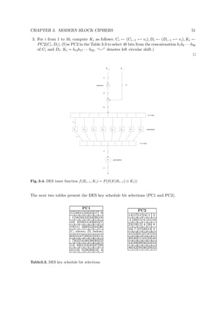
68. CHAPTER 3. MODERN BLOCK CIPHERS 62
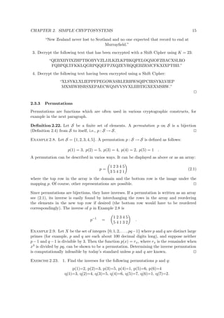
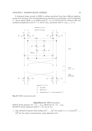
key schedules expand the 64-bit external key into 2r + 1 subkeys each of 64-bits (two for
each round plus one for the output transformation). SAFER consists entirely of simple byte
operations, aside from byte-rotations in the key schedule; it is thus suitable for processors
with small word size such as chipcards (cf. FEAL).
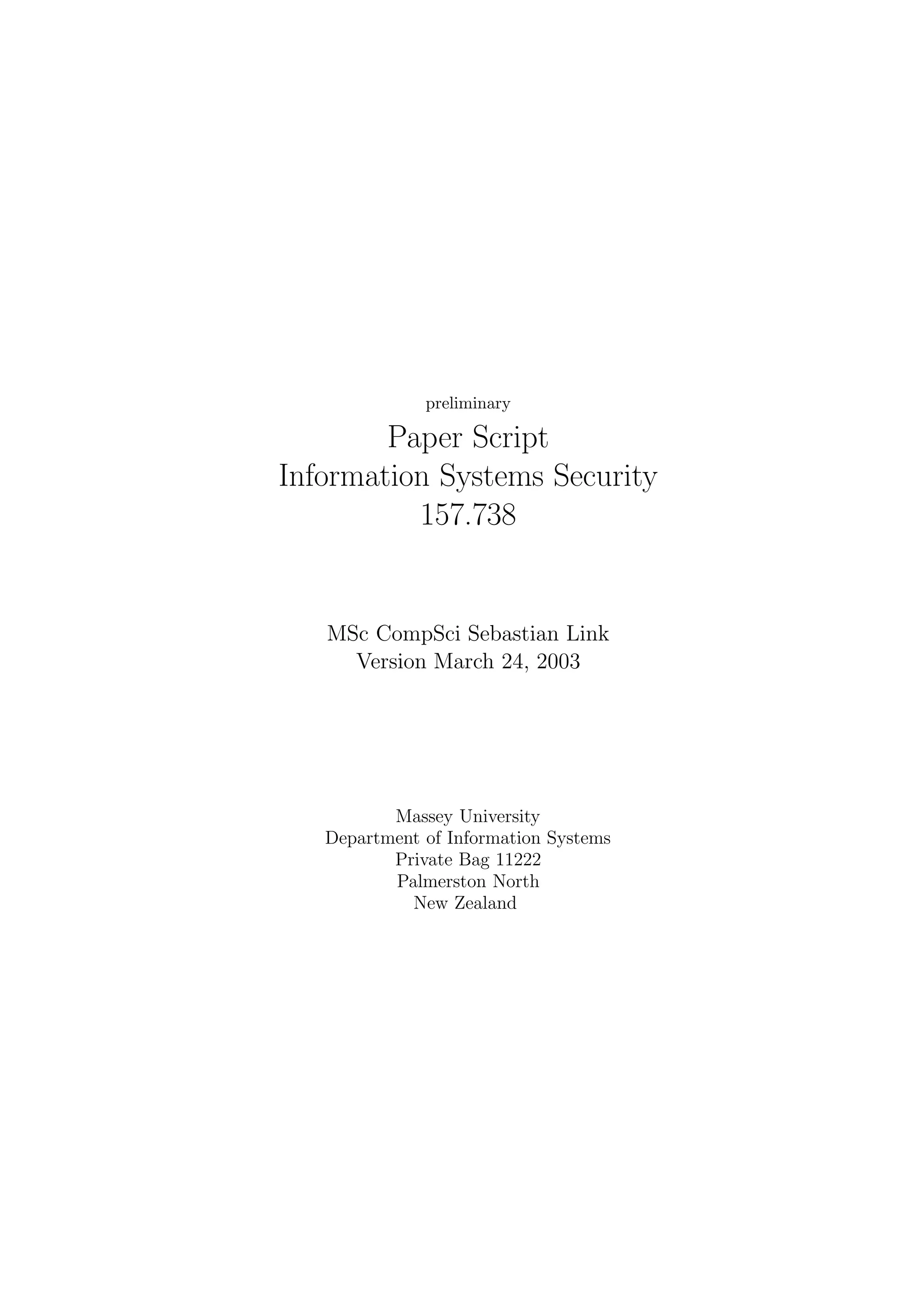
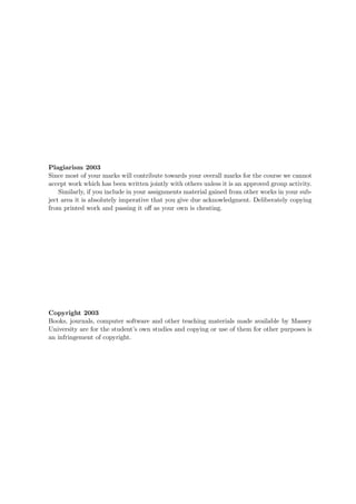
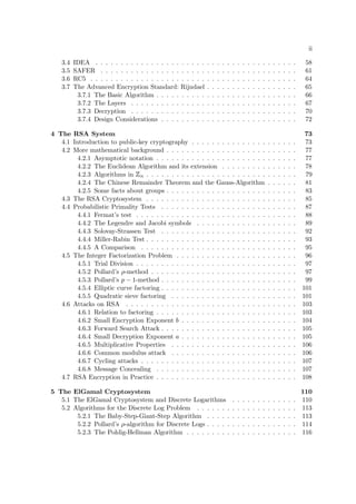
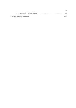
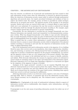
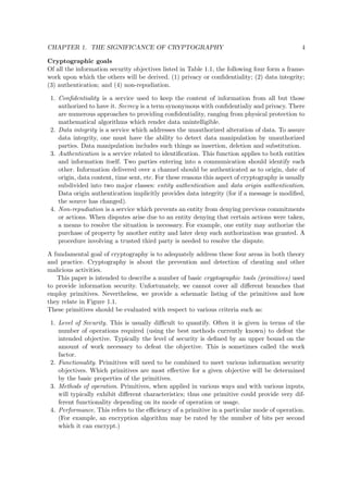
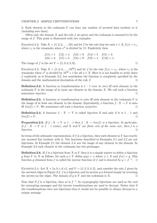
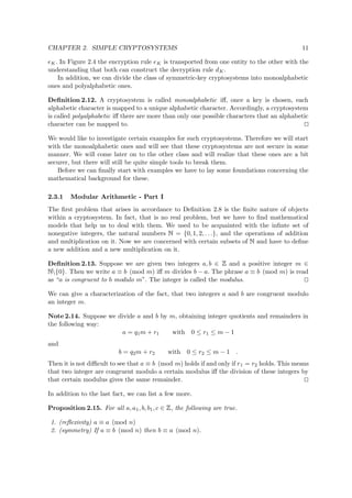
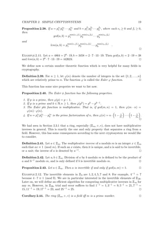
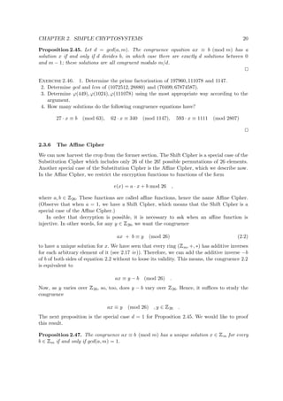
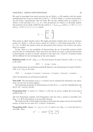
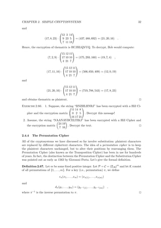
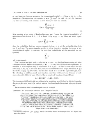
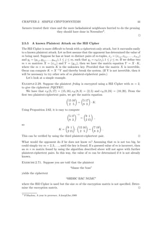
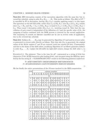
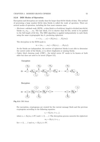
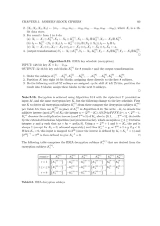
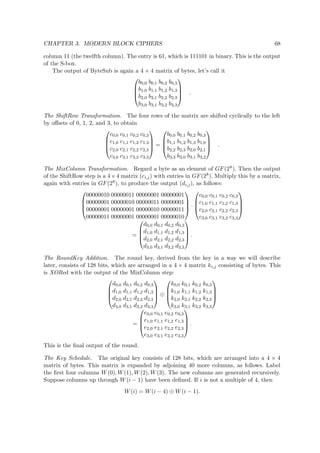
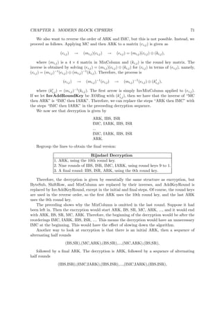
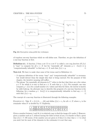
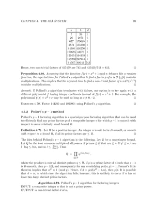
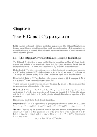
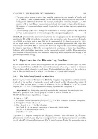
Details of SAFER K-64 are given in Algorithm 3.18 and Figure 3.8. The XOR-addition
stage beginning each round (identical to the output transformation) XORs bytes 1, 4, 5, and 8
of the (first) round subkey with the respective round input bytes, and respectively adds (mod
256) the remaining 4 subkey bytes to the others. The XOR and addition mod 256 operations
are interchanged in the subsequent addition-XOR stage. The S-boxes are an invertible byte-
to-byte substitution using one fixed 8-bit bijection. A linear transformation f (the Pseudo-
Hadamard Transform) used in the 3-level linear layer was specially constructed for rapid
diffusion. The introduction of additive key biases in the key schedule eliminates weak keys1. In
contrast to Feistel-like and many other ciphers, in SAFER the operations used for encryption
differ from those for decryption. SAFER may be viewed as an SP-network (Definition 3.3).
Algorithm 3.18 uses the following definitions (L, R denote left, right 8-bit inputs):
1. f(L, R) = (2L + R, L + R). Addition here is mod 256 (also denoted by );
2. tables S and Sinv, and the constant table for key biases Bi[j] as per Note 3.20.
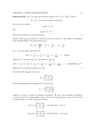
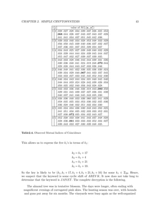
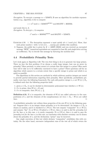
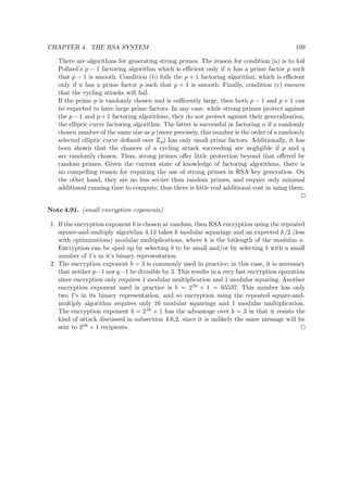
Algorithm 3.18. SAFER K-64 encryption (r rounds)
INPUT: r, 6 ≤ r ≤ 10; 64-bit plaintext M = m1 · · · m64 and key K = k1 · · · k64.
OUTPUT: 64-bit ciphertext block Y = (Y1, . . . , Y8).
1. Compute 64-bit subkeys K1, . . . , K2r+1 by algorithm 3.19 with inputs K and r.
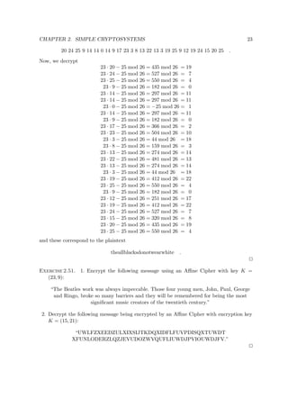
2. (X1, X2, . . . , X8) ← (m1 · · · m8, m9 · m16, . . . , m57 . . . m64).
3. For i from 1 to r do: (XOR-addition, S-box, addition - XOR, and 3 linear layers)
(a) For j = 1, 4, 5, 8 : Xj ← Xj ⊕ K2i−1[j].
For j = 2, 3, 6, 7 : Xj ← Xj K2i−1[j].
(b) For j = 1, 4, 5, 8 : Xj ← S[Xj].
For j = 2, 3, 6, 7 : Xj ← Sinv[Xj].
(c) For j = 1, 4, 5, 8 : Xj ← Xj K2i[j].
For j = 2, 3, 6, 7 : Xj ← Xj ⊕ K2i[j].
(d) For j = 1, 4, 5, 8 : (Xj, Xj+1) ← f(Xj, Xj+1).
(e) (Y1, Y2) ← f(X1, X3), (Y3, Y4) ← f(X5, X7),
(Y5, Y6) ← f(X2, X4), (Y7, Y8) ← f(X6, X8).
For j from 1 to 8 do: Xj ← Yj.
(f) (Y1, Y2) ← f(X1, X3), (Y3, Y4) ← f(X5, X7),
(Y5, Y6) ← f(X2, X4), (Y7, Y8) ← f(X6, X8).
For j from 1 to 8 do: Xj ← Yj. (This mimics the previous step.)
4. (output transformation):
For j = 1, 4, 5, 8 : Yj ← Xj ⊕ K2r+1[j]. For j = 2, 3, 6, 7 : Yj ← Xj K2r+1[j].
Algorithm 3.19. SAFER K-64 key schedule
INPUT: 64-bit key K = k1 . . . k64; number of rounds r.
OUTPUT: 64-bit subkeys K1, . . . , K2r+1. Ki[j] is byte j of Ki (numbered left to right).
1
A weak key is a key K such that eK (eK(x)) = x for all x,i.e.,defining an involution.

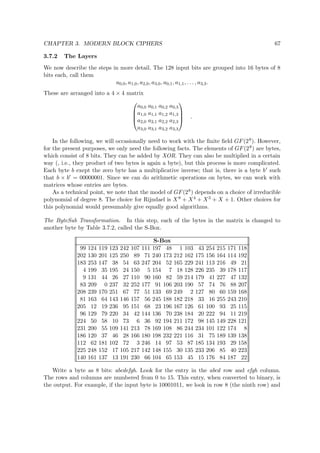
69. CHAPTER 3. MODERN BLOCK CIPHERS 63
S-1
S-1 S-1 S-1
f(x,y)=(2x y, x y)
64
64
K
1
[ 1,...,8 ]
K
2
[ 1,...,8 ]
K [ 1,...,8 ]
2i-1
K
2i
[ 1,...,8 ]
K
2r+1
[ 1,...,8 ]
64-bit ciphertext
64-bit plaintext
output
transformation(2ir)
roundi X X X X X X XX
1 2 3 4 5 6 7 8
8
8
8
S S S S
f f f f
fffff
f f f f
Y Y Y Y Y Y Y
1 2 3 4 5 6
Y
7 8
8
8
bitwise XOR
addition mod 28
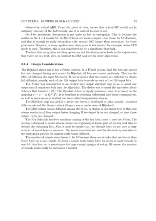
round1
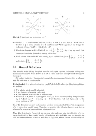
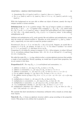
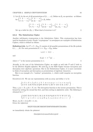
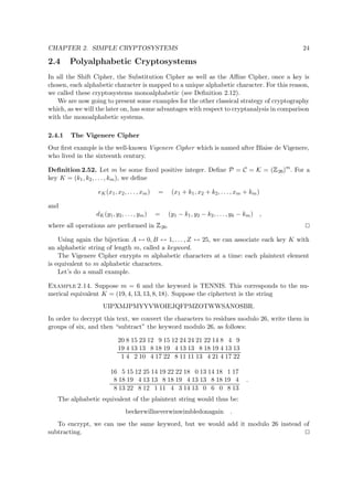
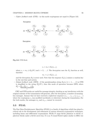
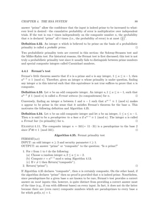
Fig. 3.8. SAFER K-64 computation path (r rounds)
1. Let R[i] denote an 8-bit data store and let Bi[j] denote byte j of Bi.
2. (R[1], R[2], . . . , R[8]) ← (k1 · · · k8, k9 . . . k16, . . . , k57 · · · k64).
3. (K1[1], K1[2], . . . , K1[8]) ← (R[1], R[2], . . . , R[8]).
4. For i from 2 to 2r + 1 do: (rotate key bytes left 3 bits, then add in the bias)
(a) For j from 1 to 8 do: R[j] ← (R[j] ← 3).
(b) For j from 1 to 8 do: Ki[j] ← R[j] Bi[j].
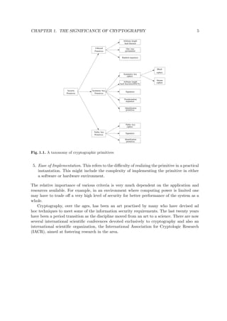
Note 3.20. The S-box, inverse S-box, and key-biases for Algorithm 3.18 are constant ta-
bles as follows. g ← 45. S[0] ← 1, Sinv[1] ← 0. For i from 1 to 255 do: t ← g · S[i − 1]
(mod 257), S[i] ← t, Sinv[t] ← i. Finally, S[128] ← 0, Sinv[0] ← 128. (Since g generates
∗
257, S[i] is a bijection on {0,1,. . . ,255}. Note that g128 ≡ 256 (mod 257), and associat-
ing 256 with 0 makes S a mapping with 8-bit input and output.) The additive key bi-

70. CHAPTER 3. MODERN BLOCK CIPHERS 64
ases are 8-bit constants used in the key schedule, intended to behave as random numbers,
and defined Bi[j] = S[S[9i + j]] for i from 2 to 2r + 1 and j from 1 to 8. For example:
B2 = (22, 115, 59, 30, 142, 112, 189, 134) and B13 = (143, 41, 221, 4, 128, 222, 231, 49).
Remark. The S-box of Note 3.20 is based on the function S(x) = gx (mod 257) using a
primitive element g = 45 ∈
257. This mapping is nonlinear with respect to both
257
arithmetic and the vector space of 8-tuples over
2 under XOR operation. The inverse S-box
is based on the base-g logarithm function.
Note 3.21. For decryption of Algorithm 3.18, the same key K and subkeys Ki are used as
for encryption. Each encryption step is undone in reverse order, from last to first. Begin
with an input transformation (XOR-subtraction stage) with key K2r+1 to undo the output
transformation, replacing modular addition with subtraction. Follow with r decryption rounds
using keys K2r through K1 (two per round), inverting each round in turn. Each starts with a
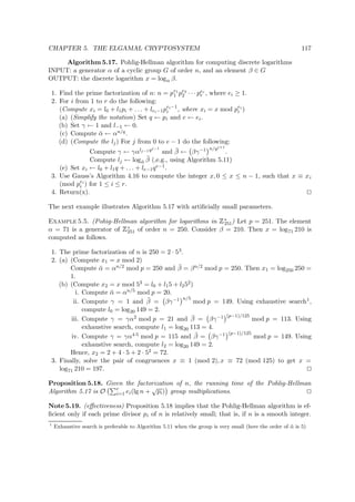
3-stage inverse linear layer using finv(L, R) = (L−R, 2R−L), with subtraction here mod 256,
in a 3-step sequence defined as follows (to invert the byte-permutations between encryption
stages):
Level 1 (for j = 1, 3, 5, 7 : (Xj, Xj+1) ← finv(Xj, Xj+1).
Level 2, 3 (each): (Y1, Y2) ← finv(X1, X5), (Y3, Y4) ← finv(X2, X6), (Y5, Y6) ← finv(X3, X7),
(Y7, Y8) ← finv(X4, X8); for j from 1 to 8 do: Xj ← Yj.
A subtraction-XOR stage follows (replace modular addition with subtraction), then an inverse
substitution stage (exchange S and S−1), and an XOR-subtraction stage.
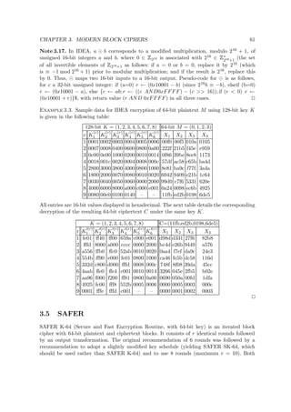
Example 3.4. Using 6-round SAFER K-64 on the 64-bit plaintext M = (1, 2, 3, 4, 5, 6, 7, 8)
with the key K = (8, 7, 6, 5, 4, 3, 2, 1) results in the ciphertext C = (200, 242, 156, 221, 135, 120,
62, 217), written as 8 bytes in decimal.
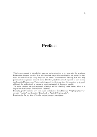
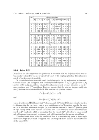
3.6 RC5
The RC5 block cipher has a word-oriented architecture for variable word sizes w = 16, 32,
or 64 bits. It has an extremely compact description, and is suitable for hardware and soft-
ware. The number of rounds r and the key-byte length b are also variable. It is successively
more completely defined as RC5-w, RC5-w/r, and RC5-w/r/b. RC5-32/12/16 is considered
a common choice of parameters; r = 12 rounds are recommended for RC5-32, and r = 16 for
RC5-64.
Algorithm 3.22 specifies RC5. Plaintext and ciphertext are blocks of bitlength 2w. Each of r
rounds updates both w-bit data halves, using 2 subkeys in an input transformation and 2 more
for each round. The only operations used, all on w-bit words, are addition mod 2w ( ), XOR
( ), and rotations (left ← and right →). The XOR operation is linear, while the addition may
be considered nonlinear depending on the metric for linearity. The datadependent rotations
featured in RC5 are the main nonlinear operation used: x ← y denotes cyclically shifting a
w-bit word left y bits; the rotation count y may be reduced mod w (the low-order lg(w) bits
of y suffice). The key schedule expands a key of b bytes into 2r + 2 subkeys Ki of w bits each.
Regarding packing/unpacking bytes into words, the byte-order is little-endian: for w = 32,
the first plaintext byte goes in the low-order end of A, the fourth in A’s high-order end, the
fifth in B’s low order end, and so on.

71. CHAPTER 3. MODERN BLOCK CIPHERS 65
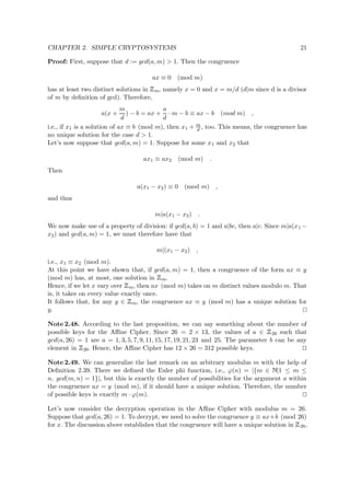
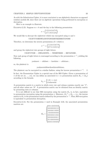
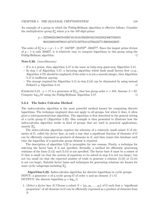
Algorithm 3.22. RC5 encryption (w-bit wordsize, r rounds, b-byte key)
INPUT: 2w-bit plaintext M = (A, B); r; key K = K[0] · · · K[b − 1].
OUTPUT: 2w-bit ciphertext C.
1. Compute 2r + 2 subkeys K0, . . . , K2r+1 by Algorithm 3.23 from inputs K and r.
2. A ← A K0, B ← B K1. (Use addition mod 2w.)
3. For i from 1 to r do: A ← ((A B) ← B) K2i, B ← ((B ⊕ A) ← A) K2i+1.
4. The output is C ← (A, B).
Algorithm 3.23. RC5 key schedule
INPUT: word bitsize w; number of rounds r; b-byte key K[0] · · · K[b − 1].
OUTPUT: subkeys K0, . . . , K2r+1 (where Ki is w bits).
1. Let u = w/8 (number of bytes per word) and c = b/u (number of words K fills). Pad
K on the right with zero-bytes if necessary to achieve a byte-count divisible by u (i.e.,
K[j] ← 0 for b ≤ j ≤ c · u − 1). For i from 0 to c − 1 do Li ←
u−1
j=0
28jK[i · u + j] (i.e., fill
Li low-order to high-order byte using each byte of K[·] once).
2. K0 ← Pw; for i from 1 to 2r + 1 do Ki ← Ki−1 Qw. (see table below.)
3. i ← 0, j ← 0, A ← 0, B ← 0, t ← max(c, 2r + 2). For s from 1 to 3t do:
(a) Ki ← (Ki A B) ← 3, A ← Ki, i ← i + 1 mod (2r + 2).
(b) Lj ← (Lj A B) ← (A B), B ← Lj, j ← j + 1 mod c.
4. The output is K0, K1, . . . , K2r+1. (The Li are not used.)
Note 3.24. Decryption uses Algorithm 3.23 subkeys, operating on ciphertext C = (A, B) as
follows (subtraction is mod 2w, denoted ). For i from r down to 1 do: B ← ((B K2i+1) →
A) ⊕ A, A ← ((A K2i) → B) ⊕ B. Finally M ← (A K0, B K1).
w : 16 32 64
Pw : B7E1 B7E15163 B7E15162 8AED2A6B
Qw : 9E37 9E3779B9 9E3779B9 7F4A7C15
Table3.6. RC5 magic constants (given as hex strings).
Example 3.5. For the hexadezimal plaintext
M = 65C178B2 84D197CC and key K = 5269F149 D41BA015 2497574D 7F153125 ,
RC5 with w = 32, r = 12, and b = 16 generates ciphertext C = EB44E415 DA319824.
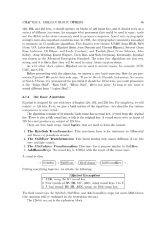
3.7 The Advanced Encryption Standard: Rijndael
In 1997, the National Institute of Standards and Technology put out a call for candidates to
replace DES. Among the requirements were that the new algorithm should allow key sizes of

72. CHAPTER 3. MODERN BLOCK CIPHERS 66
128, 192, and 256 bits, it should operate on blocks of 128 input bits, and it should work on a
variety of different hardware, for example 8-bit processors that could be used in smart cards
and the 32-bit architecture commonly used in personal computers. Speed and cryptographic
strength were also important considerations. In 1998, the cryptographic community was asked
to comment on 15 candidate algorithms. Five finalists were chosen: MARS (from IBM), RC6
(from RSA Laboratories), Rijndael (from Joan Daemen and Vincent Rijmen), Serpent (from
Ross Anderson, Eli Biham, and Lards Knudson), and Twofish (from Bruce Schneier, John
Kelsey, Doug Whiting, David Wagner, Chris Hall, and Niels Ferguson). Eventually, Rijndael
was chosen as the Advanced Encryption Standard. The other four algorithms are also very
strong, and it is likely that they will be used in many future cryptosystems.
As with other block ciphers, Rijndael can be used in several modes, for example, ECB,
CBC, and CFB.
Before proceeding with the algorithm, we answer a very basic question: How do you pro-
nounce Rijndael? We quote their web page: “If you’re Dutch, Flemish, Indonesian, Surinamer
or South-African, it’s pronounced like you think it should be. Otherwise, you could pronounce
it like “Reign Dahl”, “Rain Doll”, “Rhine Dahl”. We’re not picky. As long as you make it
sound different from “Region Deal”.”
3.7.1 The Basic Algorithm
Rijndael is designed for use with keys of lengths 128, 192, and 256 bits. For simplicity, we will
restrict to 128 bits. First, we give a brief outline of the algorithm, then describe the various
components in more detail.
The algorithm consists of 10 rounds. Each round has a round key, derived from the original
key. There is also a 0th round key, which is the original key. A round starts with an input of
128 bits and produces an output of 128 bits.
There are four basic steps, called layers, that are used to form the rounds:
1. The ByteSub Transformation: This non-linear layer is for resistance to differential
and linear cryptanalysis attacks.
2. The ShiftRow Transformation: This linear mixing step causes diffusion of the bits
over multiple rounds.
3. The MixColumn Transformation: This layer has a purpose similar to ShiftRow.
4. AddRoundKey: The round key is XORed with the result of the above layer.
A round is then
→ ByteSub → ShiftRow → MixColumn → AddRoundKey → .
Putting everything together, we obtain the following:
Rijndael Encryption
1. ARK, using the 0th round key.
2. Nine rounds of BS, SR, MC, ARK, using round keys 1 to 9.
3. A final round: BS, SR, ARK, using the 10th round key.
The final round uses the ByteSub, ShiftRow, and AddRoundKey steps but omits MixColumn
(the omission will be explained in the decryption section).
The 128-bit output is the ciphertext block.

73. CHAPTER 3. MODERN BLOCK CIPHERS 67
3.7.2 The Layers
We now describe the steps in more detail. The 128 input bits are grouped into 16 bytes of 8
bits each, call them
a0,0, a1,0, a2,0, a3,0, a0,1, a1,1, . . . , a3,3.
These are arranged into a 4 × 4 matrix




a0,0 a0,1 a0,2 a0,3
a1,0 a1,1 a1,2 a1,3
a2,0 a2,1 a2,2 a2,3
a3,0 a3,1 a3,2 a3,3



 .
In the following, we will occasionally need to work with the finite field GF(28). However,
for the present purposes, we only need the following facts. The elements of GF(28) are bytes,
which consist of 8 bits. They can be added by XOR. They can also be multiplied in a certain
way (, i.e., they product of two bytes is again a byte), but this process is more complicated.
Each byte b exept the zero byte has a multiplicative inverse; that is, there is a byte b such
that b × b = 00000001. Since we can do arithmetic operations on bytes, we can work with
matrices whose entries are bytes.
As a technical point, we note that the model of GF(28) depends on a choice of irreducible
polynomial of degree 8. The choice for Rijndael is X8 + X4 + X3 + X + 1. Other choices for
this polynomial would presumably give equally good algorithms.
The ByteSub Transformation. In this step, each of the bytes in the matrix is changed to
another byte by Table 3.7.2, called the S-Box.
S-Box
99 124 119 123 242 107 111 197 48 1 103 43 254 215 171 118
202 130 201 125 250 89 71 240 173 212 162 175 156 164 114 192
183 253 147 38 54 63 247 204 52 165 229 241 113 216 49 21
4 199 35 195 24 150 5 154 7 18 128 226 235 39 178 117
9 131 44 26 27 110 90 160 82 59 214 179 41 227 47 132
83 209 0 237 32 252 177 91 106 203 190 57 74 76 88 207
208 239 170 251 67 77 51 133 69 249 2 127 80 60 159 168
81 163 64 143 146 157 56 245 188 182 218 33 16 255 243 210
205 12 19 236 95 151 68 23 196 167 126 61 100 93 25 115
96 129 79 220 34 42 144 136 70 238 184 20 222 94 11 219
224 50 58 10 73 6 36 92 194 211 172 98 145 149 228 121
231 200 55 109 141 213 78 169 108 86 244 234 101 122 174 8
186 120 37 46 28 166 180 198 232 221 116 31 75 189 139 138
112 62 181 102 72 3 246 14 97 53 87 185 134 193 29 158
225 248 152 17 105 217 142 148 155 30 135 233 206 85 40 223
140 161 137 13 191 230 66 104 65 153 45 15 176 84 187 22
Write a byte as 8 bits: abcdefgh. Look for the entry in the abcd row and efgh column.
The rows and columns are numbered from 0 to 15. This entry, when converted to binary, is
the output. For example, if the input byte is 10001011, we look in row 8 (the ninth row) and

74. CHAPTER 3. MODERN BLOCK CIPHERS 68
column 11 (the twelfth column). The entry is 61, which is 111101 in binary. This is the output
of the S-box.
The output of ByteSub is again a 4 × 4 matrix of bytes, let’s call it




b0,0 b0,1 b0,2 b0,3
b1,0 b1,1 b1,2 b1,3
b2,0 b2,1 b2,2 b2,3
b3,0 b3,1 b3,2 b3,3



 .
The ShiftRow Transformation. The four rows of the matrix are shifted cyclically to the left
by offsets of 0, 1, 2, and 3, to obtain




c0,0 c0,1 c0,2 c0,3
c1,0 c1,1 c1,2 c1,3
c2,0 c2,1 c2,2 c2,3
c3,0 c3,1 c3,2 c3,3



 =




b0,0 b0,1 b0,2 b0,3
b1,1 b1,2 b1,3 b1,0
b2,2 b2,3 b2,0 b2,1
b3,3 b3,0 b3,1 b3,2



 .
The MixColumn Transformation. Regard a byte as an element of GF(28). Then the output
of the ShiftRow step is a 4×4 matrix (ci,j) with entries in GF(28). Multiply this by a matrix,
again with entries in GF(28), to produce the output (di,j), as follows:




00000010 00000011 00000001 00000001
00000001 00000010 00000011 00000001
00000001 00000001 00000010 00000011
00000011 00000001 00000001 00000010



 ·




c0,0 c0,1 c0,2 c0,3
c1,0 c1,1 c1,2 c1,3
c2,0 c2,1 c2,2 c2,3
c3,0 c3,1 c3,2 c3,3




=




d0,0 d0,1 d0,2 d0,3
d1,0 d1,1 d1,2 d1,3
d2,0 d2,1 d2,2 d2,3
d3,0 d3,1 d3,2 d3,3



 .
The RoundKey Addition. The round key, derived from the key in a way we will describe
later, consists of 128 bits, which are arranged in a 4 × 4 matrix ki,j consisting of bytes. This
is XORed with the output of the MixColumn step:




d0,0 d0,1 d0,2 d0,3
d1,0 d1,1 d1,2 d1,3
d2,0 d2,1 d2,2 d2,3
d3,0 d3,1 d3,2 d3,3



 ⊕




k0,0 k0,1 k0,2 k0,3
k1,0 k1,1 k1,2 k1,3
k2,0 k2,1 k2,2 k2,3
k3,0 k3,1 k3,2 k3,3




=




e0,0 e0,1 e0,2 e0,3
e1,0 e1,1 e1,2 e1,3
e2,0 e2,1 e2,2 e2,3
e3,0 e3,1 e3,2 e3,3



 .
This is the final output of the round.
The Key Schedule. The original key consists of 128 bits, which are arranged into a 4 × 4
matrix of bytes. This matrix is expanded by adjoining 40 more columns, as follows. Label
the first four columns W(0), W(1), W(2), W(3). The new columns are generated recursively.
Suppose columns up through W(i − 1) have been defined. If i is not a multiple of 4, then
W(i) = W(i − 4) ⊕ W(i − 1).

75. CHAPTER 3. MODERN BLOCK CIPHERS 69
If i is a multiple of 4, then
W(i) = W(i − 4) ⊕ T(W(i − 1)),
where T(W(i−1)) is the transformation of W(i−1) obtained as follows. Let the elements
of the column W(i − 1) be a, b, c, d. Shift these cyclically to obtain b, c, d, a. Now replace each
of these bytes with the corresponding element in the S-Box from the ByteSub step, to get 4
bytes e, f, g, h. Finally, compute the round constant
r(i) = 00000010(i−4)/4
in GF(28) (recall that we are in the case where i is a multiple of 4). Then T(W(i − 1)) is
the column vector
(e ⊕ r(i), f, g, h).
In this way, columns W(4), . . . , W(43) are generated from the initial four columns. The round
key for the ith round consists of the columns
W(4i), W(4i + 1), W(4i + 2), W(4i + 3).
The Construction of the S-Box. Although the S-Box is implemented as a lookup table, it
has a simple mathematical description. Start with the byte x7x6x5x4x3x2x1x0, which each xi
is a binary bit. Compute its inverse in GF(28). If the byte is 00000000, there is no inverse, so
we use 00000000 in place of its inverse. The resulting byte y7y6y5y4y3y2y1y0 represents an 8-
dimensional column vector, with the rightmost bit y0 is the top position. Multiply by a matrix
and add the column vector (1, 1, 0, 0, 0, 1, 1, 0) to obtain a vector (z0, z1, z2, z3, z4, z5, z6, z7) as
follows: 











1 0 0 0 1 1 1 1
1 1 0 0 0 1 1 1
1 1 1 0 0 0 1 1
1 1 1 1 0 0 0 1
1 1 1 1 1 0 0 0
0 1 1 1 1 1 0 0
0 0 1 1 1 1 1 0
0 0 0 1 1 1 1 1












·












y0
y1
y2
y3
y4
y5
y6
y7












+












1
1
0
0
0
1
1
0












=












z0
z1
z2
z3
z4
z5
z6
z7












.
The byte z7z6z5z4z3z2z1z0 is the entry for the S-Box.
For example, start with the byte 11001011. Its inverse in GF(28) is 00000100. We now
calculate 











1 0 0 0 1 1 1 1
1 1 0 0 0 1 1 1
1 1 1 0 0 0 1 1
1 1 1 1 0 0 0 1
1 1 1 1 1 0 0 0
0 1 1 1 1 1 0 0
0 0 1 1 1 1 1 0
0 0 0 1 1 1 1 1












·












0
0
1
0
0
0
0
0












+












1
1
0
0
0
1
1
0












=












1
1
1
1
1
0
0
0












.
This yields the byte 00011111. The first 4 bits 1100 represent 12 in binary and the last 4
bits 1011 represent 11 in binary. Subtract 1 from each of these numbers (since the first row

76. CHAPTER 3. MODERN BLOCK CIPHERS 70
and column are numbered 0) and look in the 11th column and 10th row of the S-Box. The
entry is 31, which in binary is 00011111.
Some of the considerations in the design of the S-Box were the following. The map x → x−1
was used to achieve nonlinearity. However, the simplicity of this map could possibly allow
certain attacks, so it was combined with multiplication by the matrix and adding the vector,
as desired previously. The matrix was chosen mostly because of its simple form (note how the
rows are shifts of each other). The vector was chosen so that no input ever equals its S-Box
output or the complement of its S-box output (complementation means changing each 1 to 0
and each 0 to 1).
3.7.3 Decryption
Each of the steps ByteSub, ShiftRow, MixColumn, and AddRoundKey is invertible:
– The inverse of ByteSub is another lookup table, called InvByteSub.
– The inverse of ShiftRow is obtained by shifting the rows to the right instead of to the
left, yielding InvShiftRow.
– The inverse of MixColumn exists because the 4×4 matrix used in MixColumn is invertible.
The transformation InvMixColumn is given by multiplication by the matrix




00001110 00001011 00001101 00001001
00001001 00001110 00001011 00001101
00001101 00001001 00001110 00001011
00001011 00001101 00001001 00001110



 .
– AddRoundKey is its own inverse.
The Rijndael encryption consists of the steps (with the obvious abbreviations)
ARK
BS,SR,MC,ARK
...
BS,SR,MC,ARK
BS,SR,ARK.
Recall that MC is missing in the last round.
To decrypt, we need to run through the inverses of these steps in the reverse order. This
yields the following preliminary version of decryption
ARK, ISR, IBS
ARK, IMC, ISR, IBS
...
ARK, IMC, ISR, IBS
ARK.
However, we want to rewrite this decryption in order to make it look more like encryption.
Observe, that applying BS then SR is the same as first applying SR then BS. This happens
because BS acts one byte at a time and SR permutes the bytes. Correspondingly, the order
of ISR and IBS can be reversed.

77. CHAPTER 3. MODERN BLOCK CIPHERS 71
We also want to reverse the order of ARK and IMC, but this is not possible. Instead, we
proceed as follows. Applying MC and then ARK to a matrix (ci,j) is given as
(ci,j) → (mi,j)(ci,j) → (ei,j) = (mi,j)(ci,j) ⊕ (ki,j),
where (mi,j) is a 4 × 4 matrix in MixColumn and (ki,j) is the round key matrix. The
inverse is obtained by solving (ei,j) = (mi,j)(ci,j) ⊕ (ki,j) for (ci,j) in terms of (ei,j), namely,
(ci,j) = (mi,j)−1(ei,j) ⊕ (mi,j)−1(ki,j). Therefore, the process is
(ei,j) → (mi,j)−1
(ei,j) → (mi,j)−1
(ei,j) ⊕ (ki,j),
where (ki,j) = (mi,j)−1(ki,j). The first arrow is simply InvMixColumn applied to (ei,j).
If we let InvAddRoundKey be XORing with (ki,j), then we have that the inverse of “MC
then ARK” is “IMC then IARK”. Therefore, we can replace the steps “ARK then IMC” with
the steps “IMC then IARK” in the preceeding decryption sequence.
We now see that decryption is given by
ARK, IBS, ISR
IMC, IARK, IBS, ISR
...
IMC, IARK, IBS, ISR
ARK.
Regroup the lines to obtain the final version:
Rijndael Decryption
1. ARK, using the 10th round key.
2. Nine rounds of IBS, ISR, IMC, IARK, using round keys 9 to 1.
3. A final round: IBS, ISR, ARK, using the 0th round key.
Therefore, the decryption is given by essentially the same structure as encryption, but
ByteSub, ShiftRow, and MixColumn are replaced by their inverses, and AddKeyRound is
replaced by InvAddKeyRound, except in the initial and final steps. Of course, the round keys
are used in the reverse order, so the first ARK uses the 10th round key, and the last ARK
uses the 0th round key.
The preceding shows why the MixColumn is omitted in the last round. Suppose it had
been left in. Then the encryption would start ARK, BS, SR, MC, ARK, ..., and it would end
with ARK, BS, SR, MC, ARK. Therefore, the beginning of the decryption would be after the
reorderings IMC, IARK, IBS, ISR, .... This means the decryption would have an unnecessary
IMC at the beginning. This would have the effect of slowing down the algorithm.
Another way to look at encryption is that there is an initial ARK, then a sequence of
alternating half rounds
(BS,SR),(MC,ARK),(BS,SR),...,(MC,ARK),(BS,SR),
followed by a final ARK. The decryption is ARK, followed by a sequence of alternating
half rounds
(IBS,ISR),(IMC,IARK),(IBS,ISR),...,(IMC,IARK),(IBS,ISR),

78. CHAPTER 3. MODERN BLOCK CIPHERS 72
followed by a final ARK. From this point of view, we see that a final MC would not fit
naturally into any of the half rounds, and it is natural to leave it out.
On 8-bit processors, decryption is not quite as fast as encryption. This is because the
entries in the 4 × 4 matrix for InvMixColumn are more complex than those for MixColumn,
and this is enough to make decryption take around 30% longer than encryption for these
processors. However, in many applications, decryption is not needed, for example, when CFB
mode is used. Therefore, this is not considered to be a significant drawback.
The fact that encryption and decryption are not identical process leads to the expectation
that there are no weak keys, in contrast to DES and several other algorithms.
3.7.4 Design Considerations
The Rijndael algorithm is not a Feistel system. In a Feistel system, half the bits are moved
but not changed during each round. In Rijndael, all bits are treated uniformly. This has the
effect of diffusing the input bits faster. It can be shown that two rounds are sufficient to obtain
full diffusion, namely, each of the 128 output bits depends on each of the 128 input bits.
The S-Box was constructed in an explicit and simple algebraic way so as to avoid any
suspicions of trapdoors bult into the algorithm. The desire was to avoid the mysteries about
S-boxes that haunted DES. The Rijndael S-box is highly nonlinear, since it is based on the
mapping x → x−1 in GF(28). It is excellent at resisting differential and linear cryptanalysis,
as well as more recently studied methods called interpolation attacks.
The ShiftRow step was added to resist two recently developed attacks, namely truncated
differentials and the Square attack (Sqaure was a predecessor of Rijndael).
The MixColumn causes diffusion among the bytes. A change in one input byte in this step
always results in all four output bytes changing. If two input bytes are changed, at least three
output bytes are changed.
The Key Schedule involves nonlinear mixing of the key bits, since it uses the S-box. The
mixing is designed to resist attacks where the cryptanalyst knows part of the key and tries to
deduce the remaining bits. Also, it aims to ensure that two distinct keys do not have a large
number of round keys in common. The round constants are used to eliminate symmetries in
the encryption process by making each round different.
The number of rounds was chosen to be 10 because there are attacks that are better than
brute force up to six rounds. No known attack beats brute force for seven or more rounds. It
was felt that four extra rounds provide large enough margin of safety. Of course, the number
of rounds could easily be increased if needed.

79. Chapter 4
The RSA System
4.1 Introduction to public-key cryptography
In the classical model of cryptography that we have been studying up to now, Alice and
Bob secretly choose the key K. K then gives rise to an encryption rule eK and a decryption
rule dK. In the cryptosystems we have seen so far, dK is either the same as eK, or easily
derived from it (for example, DES decryption is identical to encryption, but the key schedule
is reversed). Cryptosystems of this type are known as private key systems, since exposure of
eK renders the system insecure.
One drawback of a private-key system is that it requires the prior communication of the
key K between Alice and Bob, using a secure channel, before any ciphertext is transmitted.
In practice, this may be very difficult to achieve. For example, suppose Alice and Bob live far
away from each other and they decide that they want to communicate electronically, using
e-mail. In a situation such as this, Alice and Bob may not have access to a reasonable secure
channel.
The idea behind public-key system is that it might be possible to find a cryptosystem
where it is computationally infeasible to determine dK given eK. If so, then the encryption
rule eK could be made public by publishing it in a directory (hence the term public-key
system). The advantage of a public-key system is that Alice (or anyone else) can send an
encrypted message to Bob (without the prior communication of a secret key) by using the
public encryption rule eK. Bob will be the only person that can decrypt the ciphertext, using
his secret decryption rule dK.
The idea of a public-key system was due to Diffie and Hellman in 1976. They suggested
the following: Each of n ∈ {1} partner is having a public and a private key, Kp
µ and Ks
µ for
1 ≤ µ ≤ n. Kp
µ determines the encryption eKµ and Ks
µ the decryption dKµ . All keys Kp
µ are
published in a directory. The following properties must be satisfied for each µ, 1 ≤ µ ≤ n:
1. dKµ ◦ eKµ = id,
2. dKµ and eKµ can be computed in an efficent way,
3. Ks
µ and dKµ are secret and cannot be efficently determined from Kp
µ and eKµ , respectively.
Suppose, participant A (Alice) sends message m encrypted to B (Bob) using the public key
eKB
of B, i.e.,
c = eKB
(m) (4.1)

80. CHAPTER 4. THE RSA SYSTEM 74
B receives c and decrypts it to m using the private key Ks
B as follows:
dKB
(c)
(4.1)
= dKB
(eKB
(m)) = (dKB
◦ eKB
) (m)
1.
= m .
We can present this method graphically.
k
e (m)=c
e
k
d
k
decryption
Alice
unsecured channel
c
m
destination
Bob
key
sourceunsecured channel
Adversary
Passive
encryption
plaintext
source
m
d (c)=m
k
Fig. 4.1. Encryption using public-key techniques
Notice how Figure 4.1 differs from Figure 2.4 for a symmetric-key cipher. Here the encryption
key is transmitted to Alice over an unsecured channel. This unsecured channel may be the
same channel on which the ciphertext is being transmitted.
Since the encryption rule eK need not be kept secret, it may be made public. Any entity
can subsequently send encrypted messages to Bob which only Bob can decrypt. Figure 4.2
illustrates this idea, where A1, A2 and A3 are distinct entities. Note that if A1 destroys message
m1 after encrypting it to c1, then even A1 cannot recover m1 from c1.
As a physical analogue, consider a metal box with the lid secured by a combination lock.
The combination is known only to Bob. If the lock is left open and made publicly available
then anyone can place a message inside and lock the lid. Only Bob can retrieve the message.
Even the entity which placed the message into the box is unable to retrieve it.
Public-key encryption, as decribed here, assumes that knowledge of the public key eK
does not allow computation of the private key dK. In other words, this assumes the existence

81. CHAPTER 4. THE RSA SYSTEM 75
e
K
e
K
d
K
1
(m ) = c 1
e
K
A 1
3c
e
K
e
K
c 2
e
K
c 1
3
(m ) = c 3
= c 22
= m
d
K
= m
d
K
= m
(c )
(m )
1
(c )2
(c )3
1
2
3
A 2
A 3
Bob
Fig. 4.2. Encryption using public-key techniques
of trapdoor one-way functions which we will define now. Therefore, we give the definition of
a one-way function at first.
Definition 4.1. A function f from a set X to a set Y is called a one-way function iff f(x)
is “easy” to compute for all x ∈ X but for “essentially all” elements y ∈ Im(f) it is
“computationally infeasible” to find any x ∈ X such that f(x) = y.
Note 4.2. We have to make clear some of the terms used in Definition 4.1.
– A rigorous definition of the terms “easy” and “computationally infeasible” is necessary
but would detract from the simple idea that is being conveyd. For the purpose of this
chapter, the intuitive meaning will suffice.
– The phrase “for essentially all elements in Y ” refers to the fact that there are a few values
y ∈ Y for which it is easy to find an x ∈ X such that y = f(x). For example, one may
compute y = f(x) for a small number of x values and then for these, the inverse is known
by table look-up. An alternate way to describe this property of a one-way function is the
following: for a random y ∈ Im(f) it is computationally infeasible to find any x ∈ X
such that f(x) = y.
The concept of a one-way function is illustrated through the following examples.
Example 4.1. Take X = {1, 2, 3, . . . , 16} and define f(x) = rx for all x ∈ X where rx is the
remainder when 3x is divided by 17. Explicitly,
x 1 2 3 4 5 6 7 8 9 10 11 12 13 14 15 16
f(x) 3 9 10 13 5 15 11 16 14 8 7 4 12 2 6 1
.
Given a number between 1 and 16, it is relatively easy to find the image of it under f. However,
given a number such as 7, without having the table in front of you, it is harder to find x given
that f(x) = 7. Of course, if the number you are given is 3 then it is clear that x = 1 is what
you need; but for most of the elements in the codomain it is not that easy.

82. CHAPTER 4. THE RSA SYSTEM 76
One must keep in mind that this is an example, which uses very small numbers; the important
point here is that there is a difference in the amount of work to compute f(x) and the amount
of work to find x given f(x). Even for very large numbers, f(x) can be computed efficently
using the repeated square-and-multiply algorithm (which will be described later on), whereas
the process of finding x from f(x) is much harder.
Example 4.2. We select prime numbers p = 48611 and q = 53993, form n = p · q =
2624653723, and let X = {1, 2, 3, . . . , n − 1}. Define a function f on X by f(x) = rx for
each x ∈ X, where rx is the remainder when x3 is divided by n. For instance, f(2489991) =
1981394214 since 24899913 = 5881949859 · n + 1981394214. Computing f(x) is a relatively
simple thing to do, but to reverse the procedure is much more difficult; that is, given a re-
mainder to find the value x which was originally cubed. This procedure is referred to as the
computation of a modular cube root with modulus n. If the factors of n are unknown and
large, this is a difficult problem; however, if the factors p and q of n are known then there is
an efficent algorithm for computing modular cube roots.
Example 4.2 leads one to consider another type of function which will prove to be fundamental
in forthcoming developments.
Definition 4.3. A trapdoor one-way function is a one-way function f : X → Y with the
additional property that given some extra information (called the trapdoor information) it
becomes feasible to find for any given y ∈ Im(f), an x ∈ X such that f(x) = y.
Example 4.2 illustrates the concept of a trapdoor one-way function. With the additional
information of the factors of n = 2624653723 (namely, p = 48611 and q = 53993, each of
which is five decimal digits long) it becomes much easier to invert the function. The factors
of 2624653723 are large enough that finding them by hand computation would be difficult.
Of course, any reasonable computer program could find the factors relatively quickly. If, on
the other hand, one selects p and q to be very large distinct prime numbers (each having
about 100 decimal digits) then, by today’s standards, it is a difficult problem, even with the
most powerful computers, to deduce p and q simply from n. This is the well-known integer
factorization problem and a source of many trapdoor one-way functions.
It remains to be rigoursly established whether there actually are any (true) one-way func-
tions. That is to say, no one has yet definitely proved the existence of such functions under
reasonable (and rigorous) definitions of “easy” and “computationally infeasible”. Since the
existence of one-way functions is still unknown, the existence of trapdoor one-way functions
is also unknown. However, there are a number of good candidates for one-way and trapdoor
one-way functions. We are going to discuss some of the most practical ones.
Finally, we would like to conclude this introduction to public-key systems with a remark
on a possible extension of this method in general.
Remark. If we demand that the condition
4. ∀µ ∈ {1, . . . , n}. eKµ ◦ dKµ = id ,
should hold in addition to properties 1., 2. and 3., then we obtain a so-called signature schema
which works in the following way. Participant A encryptes the message m using Ks
A by
d = dKA
(m) , (4.2)

83. CHAPTER 4. THE RSA SYSTEM 77
and adds the identity ¯A. The encryption due to Ks
B yields
e = eKB
¯Ad
(4.2)
= eKB
¯AdKA
(m) (4.3)
and is sent to B. This one decrypts e with the help of Ks
B:
dKB
(e)
(4.3)
= dKB
◦ eKB
¯Ad
3.
= ¯Ad .
Having a look at the identity ¯A, B does now know that A is the message’s sender and can
continue to decrypt using
eKA
(d)
(4.2)
= eKA
◦ dKA
(m)
4.
= m .
4.2 More mathematical background
Before discussing how RSA works, we need to discuss some more facts concerning modular
arithmetic and number theory. Two fundamental results that we require are the Euclidean
Algorithm and the Chinese remainder theorem.
It is often difficult to derive the exact running time of an algorithm. In such situations
one is forced to settle for approximations of the running time, and usually may only derive
the asymptotic running time.
4.2.1 Asymptotic notation
In what follows, the only functions considered are those which are defined on the positive
integers and take on real values that are positive from some point onwards. Let f and g be
two such functions.
Definition 4.4. order notation
1. (asymptotic upper bound) f(n) = O(n) if there exists a positive constant c and a positive
integer n0 such that 0 ≤ f(n) ≤ c · g(n) for all n ≥ n0.
2. (asymptotic lower bound) f(n) = Ω(g(n)) if there exists a positive constant c and a
positive integer n0 such that 0 ≤ c · g(n) ≤ f(n) for all n ≥ n0.
3. (asymptotic tight bound) f(n) = Θ(g(n)) if there exists positive constants c1 and c2, and
a positive integer n0 such that c1g(n) ≤ f(n) ≤ c2g(n) for all n ≥ n0.
4. (o-notation) f(n) = o(g(n)) if for any positive constant c > 0 there exists a constant
n0 > 0 such that 0 ≤ f(n) < cg(n) for all n ≥ n0.
Intuitively, f(n) = O(g(n)) means that f grows no faster asymptotically than g(n) to within
a constant multiple, while f(n) = Ω(g(n)) means that f(n) grows grows at least as fast
asymptotically as g(n) to with a constant multiple. f(n) = o(g(n)) means that g(n) is an
upper bound for f(n) that is not asymptotically tight, or in other words, the function f(n)
becomes insignificant relative to g(n) as n gets larger. The expression o(1) is often used to
signify a function f(n) whose limit as n approaches ∞ is 0.
Proposition 4.5. For any functions f(n), g(n), h(n) and l(n), the following are true.

84. CHAPTER 4. THE RSA SYSTEM 78
1. f(n) = O(g(n)) if and only if g(n) = Ω(f(n)).
2. f(n) = Θ(g(n)) if and only if f(n) = O(g(n)) and f(n) = Ω(g(n)).
3. If f(n) = O(h(n)) and g(n) = O(h(n)), then (f + g)(n) = O(h(n)).
4. If f(n) = O(h(n)) and g(n) = O(l(n)), then (f · g)(n) = O(h(n)l(n)).
5. f(n) = O(f(n)).
6. If f(n) = O(g(n)) and g(n) = O(h(n)), then f(n) = O(h(n)).
4.2.2 The Euclidean Algorithm and its extension
We would first like to deal with the Euclidean Algorithm which is normally the startpoint
in courses of elementary number theory. Given two integers a and b, we want to determine
gcd(a, b). The greatest common divisor can be computed via Proposition 2.38. However, com-
puting a gcd by first obtaining prime-power factorizations does not result in an efficent algo-
rithm, as the problem of factoring integers appears to be relatively difficult. The Euclidean
Algorithm (Algorithm 4.7) is an efficient algorithm for computing the greatest common divi-
sor of two integers that does not require the factorization of the integers. It is based on the
following simple fact.
Proposition 4.6. If a and b are positive integers with a > b, then gcd(a, b) = gcd(b, a mod b).
Algorithm 4.7. Euclidean Algorithm for computing the gcd of two integers
INPUT: two non-negative integers a and b with a ≥ b.
OUTPUT: the greatest common divisor of a and b.
1. While b = 0 do the following:
Set r ← a mod b, a ← b, b ← r.
2. return(a).
Proposition 4.8. Algorithm 4.7 has a running time of O (lgn)2
bit operations.
Example 4.3. We present the steps of Algorithm 4.7 for computing gcd(4864, 3458) = 38
using long division:
4864 = 1 · 3458 + 1406
3458 = 2 · 1406 + 646
1406 = 2 · 646 + 114
646 = 5 · 114 + 76
114 = 1 · 76 + 38
76 = 2 · 38 + 0.
The Euclidean Algorithm can be extended so that it not only yields the greatest common
divisor d of two integers a and b, but also integers x and y satisfying ax + by = d. We write
x/y to denote the greatest integer which is smaller or equal to x/y.

85. CHAPTER 4. THE RSA SYSTEM 79
Algorithm 4.9. Extended Euclidean Algorithm
INPUT: two non-negative integers a and b with a ≥ b.
OUTPUT: d = gcd(a, b) and integers x, y satisfying ax + by = d.
1. If b = 0 then set d ← a, x ← 1, y ← 0, and return(d, x, y).
2. Set x2 ← 1, x1 ← 0, y2 ← 0, y1 ← 1.
3. While b > 0 do the following:
(a) q ← a/b , r ← a − qb, x ← x2 − qx1, y ← y2 − qy1.
(b) a ← b, b ← r, x2 ← x1, x1 ← x, y2 ← y1, and y1 ← y.
4. Set d ← a, x ← x2, y ← y2, and return(d, x, y).
Proposition 4.10. Algorithm 4.9 has a running time of O (lg n)2 bit operations.
Example 4.4. Table 4.2 shows the steps of algorithm 4.9 with inputs a = 4864 and b = 3458.
Hence gcd(4864, 3458) = 38 and 4864 · 32 + 3458 · (−45) = 38.
q r x y a b x2 x1 y2 y1
− − − − 4864 3458 1 0 0 1
1 1406 1 −1 3458 1406 0 1 1 −1
2 646 −2 3 1406 646 1 −2 −1 3
2 114 5 −7 646 114 −2 5 3 −7
5 76 −27 38 114 76 5 −27 −7 38
1 38 32 −45 76 38 −27 32 38 −45
2 0 −91 128 38 0 32 −91 −45 128
Table4.2. Extended Euclidean Algorithm with inputs a = 4864 and b = 3458.
Exercise 4.11. 1. Determine gcd(2574, 936) and gcd(6765, 4181).
2. Determine d = gcd(2574, 936) and (x, y) ∈
×
with x · 2574 + y · 936 = d.
3. Determine d = gcd(89, 55) and (x, y) ∈
×
with x · 89 + y · 55 = d.
4.2.3 Algorithms in
¡
Let n be a positive integer. As before, the elements of
n will be represented by integers
{0, 1, . . . , n − 1}. Observe, that if a, b ∈
n, then
(a + b) mod n =
a + b, if a + b < n,
a + b − n, if a + b ≥ n.
Hence modular addition (and subtraction) can be performed without the need of a long
division. Modular multiplication of a and b may be accomplished by simply multiplying a
and b as integers, and then taking the remainder of the result after division by n. Inverses in
n can be computed using the extended Euclidean Algorithm 4.9. We rather give a detailed
description.

86. CHAPTER 4. THE RSA SYSTEM 80
Algorithm 4.12. Computing multiplicative inverses in
n
INPUT: b ∈
n.
OUTPUT: b−1 mod n, provided it exists.
1. n0 ← n, b0 ← b, t0 ← 0, t ← 1, q ← n0/b0 , r ← n0 − q · b0
2. while r > 0 do
(a) temp ← t0 − q · t
(b) If temp ≥ 0 then temp ← temp mod n. Otherwise, temp ← n − ((−temp) mod n).
(c) t0 ← t, t ← temp, n0 ← b0, b0 ← r, q ← n0/bo , r ← n0 − q · b0.
3. If b0 = 1 then b has no inverse modulo n. Otherwise, b−1 ← t mod n, return b−1 .
Example 4.5. Suppose, we would to determine b−1 mod n with b = 17 and n = 26. Using
Algorithm 4.12 yields 17−1 = 23 mod 26. See Table 4.4 for a detailed computation. Of course,
the correctness of of one’s computation can be easily verified: you just have to determine
17 · 23 = 391 = 1 mod 26.
n0 b0 t0 t q r
26 17 0 1 1 9
17 9 1 25 1 8
9 8 25 2 1 1
8 1 2 23 8 0
Table4.4. Computation of 17−1
mod 26
Modular exponentiation can be performed efficently with the repeated square-and-multiple
algorithm (algorithm 4.13), which is crucial for many cryptographic protocols. One version
of this algorithm is based on the following observation. Let the binary representation of k be
t
i=0
ki2i, where each ki ∈ {0, 1}. Then
ak
=
t
i=0
aki2i
= a20 k0
a21 k1
· · · a2t kt
.
Algorithm 4.13. Repeated square-and-multiply algorithm for exponentiation in
n
INPUT: a ∈
n, and integer 0 ≤ k < n whose binary representation is k =
t
i=0
ki2i.
OUTPUT: ak mod n.
1. Set b ← 1. If k = 0 then return(b).
2. Set A ← a.
3. If k0 = 1 then set b ← a.
4. For i from 1 to t do the following:
(a) Set A ← A2 mod n.
(b) If ki = 1 then set b ← A · b mod n.
5. Return(b).

87. CHAPTER 4. THE RSA SYSTEM 81
i 0 1 2 3 4 5 6 7 8 9
ki 0 0 1 0 1 0 1 0 0 1
A 5 25 625 681 1011 369 421 779 947 925
b 1 1 625 625 67 67 1059 1059 1059 1013
Table4.5. Computation of 5596
mod 1234
Operation Bit Complexity
Modular Addition (a + b) mod n O(lgn)
Modular Subtraction (a − b) mod n O(lgn)
Modular multiplication (a · b) mod n O (lgn)2
Modular inversion a−1
mod n O (lgn)2
Modular exponentiation ak
mod n, k < n O (lgn)3
Table4.6. Bit complexity of basic operations in
n
Example 4.6. Table 4.5 shows the steps involved in the computation of 5596 mod 1234 =
1013.
Exercise 4.14. 1. Compute 144−1 mod 233, i.e., b = 144 and n = 233.
2. Compute 1729−1 mod 4301, i.e., b = 1729 and n = 4301.
3. Compute 54319 mod 768, i.e., a = 543, k = 19 and n = 768.
4. Compute 97263533 mod 11413, i.e., a = 9726, k = 3533 and n = 11413.
4.2.4 The Chinese Remainder Theorem and the Gauss-Algorithm
The Chinese Remainder Theorem is really a method of solving certain systems of congruences.
Suppose m1, m2, . . . , mr are pairwise relatively prime positive integers (that is, gcd(mi, mj) =
1 if i = j). Suppose a1, . . . , ar are integers, and consider the following system of congruences:
x ≡ a1 (mod m1)
x ≡ a2 (mod m2)
...
x ≡ ar (mod mr) .
The Chinese Remainder Theorem asserts that this system has a unique solution modulo
M = m1 · m2 · . . . · mr.
Theorem 4.15. If the integers m1, m2, . . . , mr are pairwise relatively prime, then the system
of simultaneous congruences
x ≡ a1 (mod m1)
x ≡ a2 (mod m2)
...
x ≡ ar (mod mr)

88. CHAPTER 4. THE RSA SYSTEM 82
has a unique solution modulo M = m1 · m2 · . . . · mr.
Proof. Proving the Chinese Remainder Theorem amounts to proving that the function
π :
M →
m1 × . . . ×
mr
x → (x mod m1, . . . , x mod mr)
is a bijection. In fact, we will be able to give an explicit formula for the inverse funtion π−1.
For 1 ≤ i ≤ r, define
Mi =
M
mi
.
Each pair mi, mj with i = j is relatively prime by assumption, i.e., the positive integers mi
and mj have no common prime factor. Therefore, the positive integers Mi = m1 · m2 · . . . ·
mi−1 · mi+1 · . . . · mr and mi have no common prime factor. According to this observation we
conclude that
gcd(Mi, mi) = 1 for all i ∈ {1, . . . , r}.
This fact together with Propostion 2.43 allow us to define
yi = M−1
i mod mi for 1 ≤ i ≤ r .
We observe that
Mi · yi ≡ 1 (mod mi) for 1 ≤ i ≤ r (4.4)
holds by definition of yi. Now we define a function
ρ :
m1 × . . . ×
mr →
M
(a1, . . . , ar) →
r
i=1
aiMiyi mod M
and show that the function ρ = π−1, i.e., it provides an explicit formula for solving the original
system of congruences.
Denote X = ρ(a1, . . . , ar), and let j ∈ {1, . . . , r}. Consider a term aiMiyi in the above
summation, reduced modulo mj. Then we distinguish two cases.
Case 1. If i = j, then we can apply the congruence (4.4) and obtain
aiMiyi ≡ ai (mod mi) .
Case 2. If i = j, then mj|Mi and we conclude
aiMiyi ≡ 0 (mod mj) .
Thus, we have that
X ≡
r
i=1
aiMiyi (mod mj)
≡ aj (mod mj) .

89. CHAPTER 4. THE RSA SYSTEM 83
Since we have chosen an arbitrary j, this congruence is true for all j, 1 ≤ j ≤ r and X is
a solution to the system of congruences.
At this point, we need to show that the solution X is unique modulo M. But this can
be done by simply counting. The function π is a function from a domain of cardinality M
to a range of cardinality M. We have just proved that π is a surjective (i.e., onto) funtion.
Hence, π must also be injective (i.e., one-to-one), since the domain and the range have the
same cardinality. It follows, that π is a bijection and π−1 = ρ. Note also, that π−1 is a linear
function of its arguments a1, . . . , ar.
Corollary 4.16. (Gauss’ algorithm) The solution x to the simultaneous congruences in the
Chinese Remainder Theorem 4.15 may be computed as x =
r
i=1
aiMiyi mod M, where Mi = M
mi
and yi = M−1
i mod mi. These computations can be performed in O (lgn)2 bit operations.
Example 4.7. Suppose, r = 3 and m1 = 5, m2 = 11 and m3 = 17. Then M = 935. We
compute M1 = 187, M2 = 85 and M3 = 55, and then y1 = 3, y2 = 7 and y3 = 13. Then the
function π−1 :
5 ×
11 ×
17 →
935 is the following:
π−1
(a1, a2, a3) = 561 · a1 + 595 · a2 + 715 · a3 mod 935 .
For example, if x ≡ 2 (mod 5), x ≡ 6 (mod 11) and x ≡ 13 (mod 17), then this formula tells
us that
x = 561 · 2 + 595 · 6 + 715 · 13 mod 935
= 13987 mod 935
= 897 mod 935 .
This can be verified by reducing 897 modulo 5, 11 and 17.
Exercise 4.17. Solve the following system of congruences
x ≡ 3 mod 5
x ≡ 1 mod 7
x ≡ 9 mod 11
x ≡ 5 mod 17.
4.2.5 Some facts about groups
We next mention some further results from elementary group theory that will be relevant in
our treatment of the RSA Cryptosystem.
Definition 4.18. For a multiplicative group G we define the order of G to be the number of
its elements. For an element g ∈ G we define the order of g to be the smallest positive integer
m such that gm = 1.

90. CHAPTER 4. THE RSA SYSTEM 84
Proposition 4.19. (Lagrange) Suppose G is a multiplicative group of order n, and g ∈ G.
Then the order of g divides n. This means that the order of a group element always divides
the group order.
We throw a glance on the algebraic structure (
n, ·).
Definition 4.20. The multiplicative group of
n is
∗
n = {a ∈
n | gcd(a, n) = 1}. In
particular, if n is prime, then
∗
n = {a | 1 ≤ a ≤ n − 1}.
It follows from the Definition of the Euler phi function (Definition 2.39) that |
∗
n |= ϕ(n).
Note also that if a ∈
∗
n and b ∈
∗
n, then a · b ∈
∗
n, and so
∗
n is closed under multiplication.
Proposition 4.21. Let n ≥ 2 be an integer.
1. (Euler’s theorem) If a ∈
∗
n, then aϕ(n) ≡ 1 (mod n).
2. If n is a product of distinct primes, and if r ≡ s (mod ϕ(n)), then ar ≡ as (mod n) for
all integers a. In other words, when working modulo such an n, exponents can be reduced
modulo ϕ(n).
A special case of Euler’s theorem is Fermat’s little theorem.
Proposition 4.22. Let p be a prime.
1. (Fermat’s theorem) If gcd(a, p) = 1, then ap−1 ≡ 1 (mod p).
2. If r ≡ s (mod p − 1), then ar ≡ as (mod p) for all integers a, st. p does not divide a. In
other words, when working modulo a prime p, exponents can be reduced modulo p − 1.
3. In particular, ap ≡ a (mod p) for all integers a.
Proposition 4.23. If the order of a ∈
∗
n is t, and as ≡ 1 (mod n), then t divides s. In
particular, t | ϕ(n).
Example 4.8. Let n = 26. Then
∗
26 = {1, 3, 5, 7, 9, 11, 15, 17, 19, 21, 23, 25}. We compute
that ϕ(26) = ϕ(2) · ϕ(13) = 12 =|
∗
26 |. The orders of elements in
∗
26 are listed in Table
4.8.
a ∈
∗
26 1 3 5 7 9 11 15 17 19 21 23 25
order of a 1 3 4 12 3 12 12 6 12 4 6 2
Table4.8. Orders of elements in
∗
26.
Definition 4.24. Let α ∈
∗
n. If the order of α is ϕ(n), then α is said to be a generator or a
primitive element of
∗
n. If
∗
n has a generator, then
∗
n is said to be cyclic.
Proposition 4.25. We list some properties of generators.
1.
∗
n has a generator iff n = 2, 4, pk or 2pk, where p is an odd prime and k ≥ 1. In particular,
if p is a prime, then
∗
p has a generator.

91. CHAPTER 4. THE RSA SYSTEM 85
2. If α is a generator of
∗
n, then
∗
n = {αi mod n | 0 ≤ i ≤ ϕ(n) − 1}.
3. Suppose that α is a generator of
∗
n. Then b = αi mod n is also a generator of
∗
n iff
gcd(i, ϕ(n)) = 1. It follows that if
∗
n is cyclic, then the number of generators is ϕ(ϕ(n)).
4. α ∈
∗
n is a generator of
∗
n if and only if αϕ(n)/p ≡ 1 (mod n) for each prime divisor p
of ϕ(n).
Example 4.9.
∗
26 is cyclic since 26 = 2·13 and 13 is an odd prime. The number of generators
is ϕ(ϕ(26)) = ϕ(12) = 4 and each element a from table 4.8 with order 12 is such a generator.
Exercise 4.26. 1. Determine
∗
18 and the order of all its elements. List its generators and
double-check their number by computing it directly.
2. Find the last base-7 digit in 21,000,000.
4.3 The RSA Cryptosystem
We are now well prepared to introduce the RSA system and to understand why it works. So,
here we go.
Definition 4.27. Let n = p · q, where p and q are distinct primes. Let P = C =
n, and
define
K = {(n, p, q, a, b) | n = pq, p, q prime, ab ≡ 1 (mod ϕ(n))}.
For K = (n, p, q, a, b), define
eK(x) = xb
mod n and dK(y) = ya
mod n
(x, y ∈
n). The values n and b are public, and the values p, q, a are secret.
This cryptosystem uses computations in
n, where n is the product of two distinct odd primes
p and q. For such n, note that ϕ(n) = (p − 1)(q − 1). We will now verify that decryption
works.
Since ab ≡ 1 (mod ϕ(n)), there is an integer k such that ab = 1 + k · ϕ(n). Now, if
gcd(x, p) = 1 then by Fermat’s theorem (Proposition 4.22),
xp−1
≡ 1 (mod p) .
We compute
xab
= x1+k·ϕ(n)
= x1+k·(p−1)·(q−1)
= x · xp−1 k·(q−1)
≡ x (mod p)
and therefore, xab ≡ x (mod p). On the other hand, if gcd(x, p) = p, then this last congruence
is again valid since each side is congruent 0 modulo p. Hence, in all cases
xab
≡ x (mod p) .
By the same argument,
xab
≡ x (mod q) .
By definition, there must be two integers r and s such that xab − x = p · r = q · s. Since p and
q are distinct and prime, p must be a factor of s due to the unique prime factorization (or q

92. CHAPTER 4. THE RSA SYSTEM 86
must be a factor of r). Again, there has to be an integer s such that xab − x = qs = qps , i.e.
n = p · q divides xab − x or in other words
xab
≡ x (mod n) .
Therefore,
dK (eK(x)) = dK xb
mod n = xb
mod n
a
mod n = xab
mod n = x mod n
which means that the RSA system works. Note, that also eK (dK(x)) = x in
n, i.e., the RSA
system can also be used to set up a signature scheme.
The security of RSA is based on the hope that the encryption function eK(x) = xb mod n
is one-way, so it will be computationally infeasible for an opponent to decrypt a ciphertext.
The trapdoor that allows Bob to decrypt is the knowledge of the factorization n = p·q. Since
Bob knows this factorization, he can compute ϕ(n) = (p−1)·(q −1) and then the decryption
exponent a using Algorithm 4.12.
Algorithm 4.28. Key generation for RSA public-key encryption
SUMMARY: each entity creates an RSA public key and a corresponding private key.
Each entity A should do the following:
1. Generate two large random (and distinct) primes p and q, each roughly the same size.
2. Compute n = p · q and ϕ(n) = (p − 1) · (q − 1).
3. Select a random integer b, 1 < b < ϕ(n) such that gcd(b, ϕ(n)) = 1.
4. Use Algorithm 4.12 to compute the unique integer a, 1 < a < ϕ(n), such that ab ≡ 1
(mod ϕ(n)).
5. A’s public key is (n, b); A’s private key is a.
The integers a and b are called the encryption exponent and the decryption exponent, respec-
tively, while n is called the modulus.
Algorithm 4.29. RSA public-key encryption
SUMMARY: B encrypts a message m for A, which A decrypts.
1. Encryption. B should do the following:
(a) Obtain A’s authentic public key (n, b).
(b) Represent the message as an integer m in the set {0, . . . , n − 1}.
(c) Compute c = mb mod n using Algorithm 4.13.
(d) Send the ciphertext c to A.
2. Decryption. To recover plaintext m from c, A should do the following:
(a) Use the private key a to recover m = ca mod n.
Example 4.10. We do an RSA encryption with artificially small parameters.
Key generation. Entity A chooses the primes p = 2357, q = 2551, and computes n =
pq = 6012707 and ϕ(n) = (p − 1)(q − 1) = 6007800. A chooses b = 3674911 and, us-
ing algorithm 4.12, finds a = 422191 such that ab ≡ 1 mod ϕ(n). A’s public key pair is
(n = 6012707, b = 3674911), while A’s private key is a = 422191.

93. CHAPTER 4. THE RSA SYSTEM 87
Encryption. To encrypt a message m = 5234673, B uses an algorithm for modular exponen-
tiation (e.g., algorithm 4.13) to compute
c = mb
mod n = 52346733674911
mod 6012707 = 3650502,
and sends this to A.
Decryption. To decrypt c, A computes
ca
mod n = 3650502422191
mod 6012707 = 5234673.
Exercise 4.30. 1. The decryption exponent a must satisfy ab ≡ 1 mod ϕ(n). Show, that
each prime number r with r ∈ {1, 2, 3, . . . , max{p, q}} satisfies this condition.
2. Suppose, the public key is given by K = (46927, 39423) and you received an encrypted
message “BFIC” (numerical equivalents are computed to base 26, each single letter serving
as coefficient). Try to decode this message by factoring the modulus first.
4.4 Probabilistic Primality Tests
Let’s look again at Algorithm 4.28. The very first thing to do is to generate two large primes.
There we face the first problem: if we choose a really large integer, how can we prove its
primality? More precisely, to what extent is it certain that this integer is a prime? How much
time will it take us to be sufficently convinced to have a prime? These questions call for an
algorithm which assures to a certain extent that a specific integer is prime and which is as
quick as possible.
The algorithms in this section are methods by which arbitrary positive integers are tested
to provide partial information regarding their primality. More specifically, probabilistic pri-
mality tests have the following framework. For each odd positive integer n, a set W(n) ⊆
n
is defined such that the following properties hold:
1. given a ∈
n, it can be checked in deterministic polynomial time whether a ∈ W(n);
2. if n is prime, then W(n) = ∅; and
3. if n is composite, then |W(n)| ≥ n
2 .
Definition 4.31. If n is composite, the elements of W(n) are called witnesses to the com-
positeness of n, and the elements of the complementary set L(n) =
n − W(n) are called
liars.
A probabilistic primality test utilizes these properties of the sets W(n) in the following man-
ner. Suppose that n is an integer whose primality is to be determined. An integer a ∈
n is
chosen at random, and it is checked if a ∈ W(n). The test outputs “composite” if a ∈ W(n),
and outputs “liar” if a ∈ W(n). If indeed a ∈ W(n), then a is said to fail the primality test
for the base a; in this case, n is surely composite. If a ∈ W(n), then n is said to pass the
primality test for the base a; in this case, no conclusion with absolute certainty can be drawn
about the primality of n, and the declaration “prime” may be incorrect.
Any single execution of this test which declares “composites” establishes this with cer-
tainty. On the other hand, successive independent runs of the test all of which return the

94. CHAPTER 4. THE RSA SYSTEM 88
answer “prime” allow the confidence that the input is indeed prime to be increased to what-
ever level is desired—the cumulative probability of error is multiplicative over independent
trials. If the test is run t times independently on the composite number n, the probability
that n is declared “prime” all t times (i.e., the probability of error) is at most 1
2
t
.
Definition 4.32. An integer n which is believed to be prime on the basis of a probabilistic
primality is called a probable prime.
Two probabilistic primality tests are covered in this section: the Solovay-Strassen test and
the Miller-Rabin test. For historical reasons, the Fermat test is first discussed; this test is not
truly a probabilistic primality test since it usually fails to distinguish between prime numbers
and special composite integers called Carmichael numbers.
4.4.1 Fermat’s test
Fermat’s little theorem asserts that if n is a prime and a is any integer, 1 ≤ a ≤ n − 1, then
an−1 ≡ 1 (mod n). Therefore, given an integer n whose primality is under question, finding
any integer a in this interval such that this equivalence is not true suffices to prove that n is
composite.
Definition 4.33. Let n be an odd composite integer. An integer a, 1 ≤ a ≤ n − 1, such that
an−1 ≡ 1 (mod n) is called a Fermat witness (to compositeness) for n.
Conversely, finding an integer a between 1 and n − 1 such that an−1 ≡ 1 (mod n) makes
n appear to be prime in the sense that it satisfies Fermat’s theorem for the base a. This
motivates the following definition and Algorithm 4.35.
Definition 4.34. Let n be an odd composite integer and let a be an integer, 1 ≤ a ≤ n − 1.
Then n is said to be a pseudoprime to a base a if an−1 ≡ 1 (mod n). The integer a is called
a Fermat liar (to primality) for n.
Example 4.11. The composite integer n = 341(= 11 · 31) is a pseudoprime to the base 2
since 2340 ≡ 1 (mod 341).
Algorithm 4.35. Fermat primality test
FERMAT(n,t)
INPUT: an odd integer n ≥ 3 and security parameter t ≥ 1.
OUTPUT: an answer “prime” or “composite” to the question: “Is n prime?”
1. For i from 1 to t do the following:
(a) Choose a random integer a, 2 ≤ a ≤ n − 2.
(b) Compute r = an−1 mod n using Algorithm 4.13.
(c) If r = 1 then Return(“composite”).
2. Return(“prime”).
If Algorithm 4.35 declares “composite”, then n is certainly composite. On the other hand, if
the algorithm declares “prime” then no proof is provided that n is indeed prime. Nonetheless,
since pseudoprimes for a given base a are known to be rare, Fermat’s test provides a correct
answer on most inputs; this, however, is quite distinct from providing a correct answer most
of the time (e.g., if run with different bases) on every input. In fact, it does not do the latter
because there are (even rarer) composite numbers which are pseudoprimes to every base a
for which gcd(a, n) = 1.

95. CHAPTER 4. THE RSA SYSTEM 89
Definition 4.36. A Carmichael number n is a composite integer such that an−1 ≡ 1 (mod n)
for all integers a which satisfy gcd(a, n) = 1.
If n is a Carmichael number, then the only Fermat witnesses for n are those integers a, 1 ≤
a ≤ n−1, for which gcd(a, n) > 1. Thus, if the prime factors of n are all large, then with high
probability the Fermat test declares that n is “prime”, even if the number of iterations t is
large. This deficiency in the Fermat test is removed in the Solovay-Strassen and Miller-Rabin
probabilistic primality test by relying on criteria which are stronger than Fermat’s theorem.
This subsection is concluded with some facts about Carmichael numbers. If the prime
factorization of n is known, then the Proposition 4.37 can be used to easily determine whether
n is a Carmichael number.
Proposition 4.37. A composite integer n is a Carmichael number if and only if the following
two conditions are satisfied:
1. n is square-free, i.e., n is not divisible by the square of any prime; and
2. p − 1 divides n − 1 for every prime divisor p of n.
Proposition 4.38. Every Carmichael number is the product of at least three distinct primes.
Example 4.12. The Carmichael numbers under 100,000 are 561, 1105, 1729, 2465, 2821, 6601,
8911, 10585, 15841, 29341, 41041, 46657, 52633, 62745, 63973, and 75361.
Small Carmichael numbers are rare: there are only 2,163 are less than 25,000,000,000. Re-
cently, Richard Pinch has found that there are still only 246,683 Carmichael numbers below
10,000,000,000,000,000. Nevertheless, in 1994 it was proved that there are infinitely many of
them!
Exercise 4.39. Proof, that 561 and 1105 are indeed Carmichael numbers.
4.4.2 The Legendre and Jacobi symbols
The Solovay-Strassen algorithm employs mathematical background we have not introduced
so far. That is, what we want to do in this section.
The Legendre symbol is a useful tool for keeping track of whether or not an integer a is a
quadratic residue modulo a prime p.
Definition 4.40. Let a ∈
∗
n. a is said to be a quadratic residue modulo n, or a square modulo
n, if there exists an x ∈
∗
n such that x2 ≡ a (mod n). If no such x exists, then a is called
a quadratic non-residue modulo n. The set of all quadratic residues modulo n is denoted by
Qn and the set of all quadratic non-residues is denoted by ¯Qn.
Note that by definition 0 ∈
∗
n, whence 0 ∈ Qn and 0 ∈ ¯Qn.
Proposition 4.41. Let p be an odd prime and let α be a generator of
∗
p. Then a ∈
∗
p is a
quadratic residue modulo p if and only if a = αi mod p, where i is an even integer. It follows
that | Qp |= (p − 1)/2 and | ¯Qp |= (p − 1)/2; that is, half of the elements in
∗
p are quadratic
residues and the other half are quadratic non-residues.

96. CHAPTER 4. THE RSA SYSTEM 90
Example 4.13. α = 6 is a generator of
∗
13. The powers of α are listed in the following table.
i 0 1 2 3 4 5 6 7 8 9 10 11
αi mod 13 1 6 10 8 9 2 12 7 3 5 4 11
Hence Q13 = {1, 3, 4, 9, 10, 12} and ¯Q13 = {2, 5, 6, 7, 8, 11}.
Proposition 4.42. Let n be a product of two distinct odd primes p and q, n = pq. Then
a ∈
∗
n is a quadratic residue modulo n if and only if a ∈
∗
p and a ∈
∗
q. It follows that
| Qn |=| Qp | · | Qq |= (p − 1)(q − 1)/4 and | ¯Qn |= 3(p − 1)(q − 1)/4.
Example 4.14. Let n = 21. Then Q21 = {1, 4, 16} and ¯Q21 = {2, 5, 8, 10, 11, 13, 17, 19, 20}.
Definition 4.43. Let p be an odd prime and a an integer. The Legendre symbol a
p is defined
to be
a
p
=



0, if p | a,
1, if a ∈ Qp,
−1, if a ∈ ¯Qp.
Proposition 4.44. Let p be an odd prime and a, b ∈
. Then the Legendre symbol has the
following properties:
1. a
p ≡ a(p−1)/2 (mod p). In particular, 1
p = 1 and −1
p = (−1)(p−1)/2. Hence −1 ∈ Qp
if p ≡ 1 (mod 4), and −1 ∈ ¯Qp if p ≡ 3 (mod 4).
2. ab
p = a
p · b
p . Hence if a ∈
∗
p, then a2
p = 1.
3. If a ≡ b (mod p), then a
p = b
p .
4. 2
p = (−1)(p2−1)/8. Hence 2
p = 1 if p ≡ 1 or 7 (mod 8), and 2
p = −1 if p ≡ 3 or 5
(mod 8).
5. (law of quadratic reciprocity) If q is an odd prime distinct from p, then
p
q
=
q
p
(−1)(p−1)(q−1)/4
.
In other words, p
q = q
p unless both p and q are congruent to 3 modulo 4, in which
case p
q = − q
p .
The Jacobi symbol is a generalization of the Legendre symbol to integers n which are odd
but not necessarily prime.
Definition 4.45. Let n ≥ 3 be odd with prime factorization n = pe1
1 pe2
2 ·pek
k . Then the Jacobi
symbol a
n is defined to be
a
n
=
a
p1
e1
a
p2
e2
· · ·
a
pk
ek
.

97. CHAPTER 4. THE RSA SYSTEM 91
Observe that if n is prime, then the Jacobi symbol is just the Legendre symbol.
Proposition 4.46. Let m ≥ 3, n ≥ 3 be odd integers, and a, b ∈
. Then the Jacobi symbol
has the following properties:
1. a
n = 0, 1 or −1. Moreover, a
n = 0 if and only if gcd(a, n) = 1.
2. ab
n = a
n
b
n . Hence if a ∈
∗
n, then a2
n = 1.
3. a
mn = a
m
a
n .
4. If a ≡ b (mod n), then a
n = b
n .
5. 1
n = 1.
6. −1
n = (−1)(n−1)/2. Hence −1
n = 1 if n ≡ 1 (mod 4), and −1
n = −1 if n ≡ 3 (mod 4).
7. 2
n = (−1)(n2−1)/8. Hence 2
n = 1 if n ≡ 1 or 7 (mod 8), and 2
n = −1 if n ≡ 3 or 5
(mod 8).
8. m
n = n
m (−1)(m−1)(n−1)/4. In other words, m
n = n
m unless both m and n are con-
gruent 3 modulo 4, in which case m
n = − n
m .
By properties of the Jacobi symbol it follows that if n is odd and a = 2ea1 where a1 is odd,
then
a
n
=
2e
n
a1
n
=
2
n
e
n mod a1
a1
(−1)(a1−1)(n−1)/4
.
This observation yields the following recursive algorithm for computing a
n , which does not
require the prime factorization of n.
Algorithm 4.47. Jacobi symbol (and Legendre symbol) computation
JACOBI(a,n)
INPUT: an odd integer n ≥ 3, and an integer a, 0 ≤ a < n.
OUTPUT: the Jacobi symbol a
n (and hence the Legendre symbol when n is prime).
1. If a = 0 then return(0).
2. If a = 1 then return(1).
3. Write a = 2ea1, where a1 is odd.
4. If e is even, then set s ← 1. Otherwise set s ← 1 if n ≡ 1 or 7 (mod 8), or set s ← −1 if
n ≡ 3 or 5 (mod 8).
5. If n ≡ 3 (mod 4) and a1 ≡ 3 (mod 4) then set s ← −s.
6. Set n1 ← n mod a1.
7. If a1 = 1 then return(s); otherwise return(s · JACOBI(n1, a1)).
Proposition 4.48. Algorithm 4.47 has a running time of O (lgn)2 bit operations.
Remark. Let p denote an odd prime. Even though it is known that half of the elements in
∗
p are quadratic non-residues modulo p, there is no deterministic polynomial-time algorithm
known for finding one. A randomized algorithm for finding a quadratic non-residue is to
simply select random integers a ∈
∗
p until one is found satisfying a
p = −1. The expected
number iterations before a non-residue is found is 2, and hence the procedure takes expected
polynomial-time.

98. CHAPTER 4. THE RSA SYSTEM 92
Example 4.15. For a = 158 and n = 235, Algorithm 4.47 computes the Jacobi symbol 158
235
as follows:
158
235 = 2
235
79
235
= (−1) 235
79 (−1)78·234/4
= 77
79
= 79
77 (−1)76·78/4
= 2
77
= −1.
Unlike the Legendre symbol, the Jacobi symbol a
n does not reveal whether or not a is a
quadratic residue modulo n. It is indeed true that if a ∈ Qn, then a
n = 1. However, a
n = 1
does not imply that a ∈ Qn.
Example 4.16. We list the elements of
∗
21 and their Jacobi symbols. Recall from example
4.14 that Q21 = {1, 4, 16}. Observe that 5
21 = 1 but 5 /∈ Q21.
a ∈
∗
21 1 2 4 5 8 10 11 13 16 17 19 21
a2 mod n 1 4 16 4 1 16 16 1 4 16 4 1
a
3 1 −1 1 −1 −1 1 −1 1 1 −1 1 −1
a
7 1 1 1 −1 1 −1 1 −1 1 −1 −1 −1
a
21 1 −1 1 1 −1 −1 −1 −1 1 1 −1 1
Exercise 4.49. Determine 78
133 and 7411
9283 .
4.4.3 Solovay-Strassen Test
The Solovay-Strassen probabilistic primality test was the first such test popularized by the
advent of public-key cryptography, in particular the RSA cryptosystem. There is no longer
any reason to use this test, because an alternative is available (Miller-Rabin test) which is both
more efficent and always at least as correct. Discussion is nonetheless included for historical
completeness and to clarify this exact point, since many people continue to reference this
test. The Solovay-Strassen test is based on the following fact, which is known as Euler’s
criterion.
Proposition 4.50. Let n be an odd prime. Then a(n−1)/2 ≡ a
n (mod n) for all integers a
which satisfy gcd(a, n) = 1.
Definition 4.51. Let n be an odd composite integer and let a be an integer 1 ≤ a ≤ n − 1.
1. If either gcd(a, n) > 1 or a(n−1)/2 ≡ a
n (mod n), then a is called an Euler witness (to
compositeness) for n.
2. Otherwise, i.e., if gcd(a, n) = 1 and a(n−1)/2 ≡ a
n (mod n), then n is said to be an
Euler pseudoprime to the base a. (That is, n acts like a prime in that it satisfies Euler’s
criterion for the particular base a). The integer a is called Euler liar (to primality) for
n.

99. CHAPTER 4. THE RSA SYSTEM 93
Example 4.17. The composite integer 91 (= 7 · 13) is an Euler pseudoprime to the base 9
since 945 ≡ 1 (mod 91) and 9
91 = 1.
Euler’s criterion can be used as a basis for a probabilistic primality test because of the
following result.
Proposition 4.52. Let n be an odd composite integer. Then at most ϕ(n)/2 of all the numbers
a, 1 ≤ a ≤ n − 1 are Euler liars for n. Here, ϕ is the Euler ϕ function.
Algorithm 4.53. Solovay-Strassen probabilitic primality test
SOLOVAY-STRASSEN(n,t)
INPUT: an odd integer n ≥ 3 and security parameter t ≥ 1.
OUTPUT: an answer ”prime” or ”composite” to the question: ”Is n prime?”
1. For i from 1 to t do the following:
(a) Choose a random integer a, 2 ≤ a ≤ n − 2.
(b) Compute r = a(n−1)/2 mod n using Algorithm 4.13.
(c) If r = 1 and r = n − 1 then return(”composite”).
(d) Compute the Jacobi symbol s = a
n using Algorithm 4.47.
(e) If r ≡ s (mod n) then return(”composite”).
2. Return(”prime”).
If gcd(a, n) = d, then d is a divisor of r = a(n−1)/2 mod n. Hence, testing whether r = 1
is step 1.(c), eliminates the necessity of testing whether gcd(a, n) = 1. If Algorithm 4.53
declares ”composite”, then n is certainly composite because prime numbers do not violate
Euler’s criterion. Equivalently, if n is actually prime, then the algorithm always declares
”prime”. On the other hand, if n is actually composite, then since the bases a in step 1.(a)
are chosen independently during each iteration of step 1, Proposition 4.52 can be used to
deduce the following probability of the algorithm erroneously declaring ”prime”.
Proposition 4.54. (Solovay-Strassen error-probability bound) Let n be an odd composite in-
teger. The probability that SOLOVAY-STRASSEN(n,t) declares n to be ”prime” is less than
1
2
t
.
Exercise 4.55. Determine all Euler Liars for 21.
4.4.4 Miller-Rabin Test
The probabilistic primality test used most in practice is the Miller-Rabin test, also known as
the strong pseudoprime test. The test is based on the following fact.
Proposition 4.56. Let n be an odd prime, and let n − 1 = 2sr where r is odd. Let a be any
integer such that gcd(a, n) = 1. Then either ar ≡ 1 (mod n) or a2j r ≡ −1 (mod n) for some
j, 0 ≤ j ≤ s − 1.
Definition 4.57. Let n be an odd composite integer and let n − 1 = 2sr where r is odd. Let
a be an integer in the set {1, . . . , n − 1}.
1. If ar ≡ 1 (mod n) and if a2j r ≡ −1 (mod n) for all j, 0 ≤ j ≤ s − 1, then a is called a
strong witness (to compositeness) for n.

100. CHAPTER 4. THE RSA SYSTEM 94
2. Otherwise, i.e., if either ar ≡ 1 (mod n) or a2j r ≡ −1 (mod n) for some j, 0 ≤ j ≤ s − 1,
then n is said to be a strong pseudoprime to the base a. (That is, n acts like a prime
in that it satisfies Proposition 4.56) for the particular base a.) The integer a is called a
strong liar (to primality) for n.
Example 4.18. Consider the composite integer n = 91 (= 7 · 13). Since 91 − 1 = 90 =
2 · 45, s = 1 and r = 45. Since 9r = 945 ≡ 1 (mod 91), 91 is a strong pseudoprime to the base
9. The set of all strong liars for 91 is:
{1, 9, 10, 12, 16, 17, 22, 29, 38, 53, 62, 74, 75, 79, 81, 82, 90} .
Notice that the number of strong liars for 91 is 18 = ϕ(91)/4, where ϕ is the Euler ϕ function.
Proposition 4.56 can be used as a basis for a probabilistic primality test due to the following
result.
Proposition 4.58. If n is an odd composite integer, then at most 1
4 of all the numbers a, 1 ≤
a ≤ n − 1, are strong liars for n. In fact, if n = 9, the number of strong liars for n is at most
ϕ(n)/4, where ϕ is the Euler ϕ function.
Algorithm 4.59. Miller-Rabin probabilistic primality test
MILLER-RABIN(n,t)
INPUT: an odd integer n ≥ 3 and security parameter t ≥ 1.
OUTPUT: an answer ”prime” or ”composite” to the question: ”Is n prime?”
1. Write n − 1 = 2sr such that r is odd.
2. For i from 1 to t do the following:
(a) Choose a random integer a, 2 ≤ a ≤ n − 2.
(b) Compute y = ar mod n using Algorithm 4.13.
(c) If y = 1 and y = n − 1 then do the following:
j ← 1.
While j ≤ s − 1 and y = n − 1 do the following:
Compute y ← y2 mod n.
If y = 1 then return(”composite”).
j ← j + 1
If y = n − 1 then return(”composite”).
3. Return(”prime”).
Algorithm 4.59 tests whether each base a satisfies the conditions of Definition 4.57, 1. In
the fifth line of step 2.(c), if y = 1, then a2j r ≡ 1 (mod n). Since it is also the case that
a2j−1r ≡ ±1 (mod n), it follows that n is composite (in fact, gcd(a2j−1r −1, n) is a non-trivial
factor of n 1). In the seventh line of step 2.(c), if y = n−1, then a is a strong witness for n. If
Algorithm 4.59 declares ”composite”, then n is certainly composite because prime numbers
do not violate Proposition 4.56. Equivalently, if n is actually prime, then the algorithm always
declares ”prime”. On the other hand, if n is actually composite, then Proposition 4.58 can be
used to deduce the following probability of the algorithm erroneously declaring ”prime”.
1
we omitted the following result: Let x, y and n be integers. If x2
≡ y2
(mod n) but x ≡ ±y (mod n), then
gcd(x − y, n) is a non-trivial factor of n.

101. CHAPTER 4. THE RSA SYSTEM 95
Proposition 4.60. (Miller-Rabin error-probability bound) For any odd composite integer n,
the probability that MILLER-RABIN(n,t) declares n to be ”prime” is less than 1
4
t
.
4.4.5 A Comparison
The following result describes the relationship between Fermat liars, Euler liars and strong
liars.
Proposition 4.61. Let n be an odd composite integer.
– If a is an Euler liar for n, then it is also a Fermat liar for n.
– If a is a strong liar for n, then it is also an Euler liar for n.
Example 4.19. Consider the composite integer n = 65 (= 5·13). The Fermat liars for 65 are
{1, 8, 12, 14, 18, 21, 27, 31, 34, 38, 44, 47, 51, 53, 57, 64}. The Euler liars for 65 are {1, 8, 14, 18,
47, 51, 57, 64}, while the strong liars for 65 are {1, 8, 18, 47, 57, 64}.
For a fixed composite candidate n, the situation is depicted in Figure 4.3.
strong liars for n
Euler liars for n
Fermat liars for n
Fig. 4.3. Relationship between Fermat, Euler and strong liars for a composite integer n.
This settles the question of the relative accuracy of the Fermat, Solovay-Strassen and
Miller-Rabin tests, not only in the sense of the relative correctness of each test on a fixed
candidate n, but also in the sense that given n, the specified containments hold for each
randomly chosen base a. Thus, from a correctness point of view, the Miller-Rabin test is
never worse than the Solovay-Strassen test, which in turn is never worse than the Fermat
test. As the following result shows, there are, however, some composite integers n for which
the Solovay-Strassen and Miller-Rabin test are equally good.
Proposition 4.62. If n ≡ 3 (mod 4), then a is an Euler liar for n if and only if it is a strong
liar for n.
What remains is a comparison of the computational costs. While the Miller-Rabin test may
appear more complex, it actually requires, at worst, the same amount of computation as
Fermat’s test in terms of modular multiplications; thus the Miller-Rabin test is better than
Fermat’s test in all regards. At worst, the sequence of computation defined in MILLER-
RABIN(n,1) requires the equivalent of computing a(n−1)/2 mod n. It is also the case that

102. CHAPTER 4. THE RSA SYSTEM 96
MILLER-RABIN(n,1) requires less computation than SOLOVAY-STRASSEN(n,1), the lat-
ter requiring the computation of a(n−1)/2 mod n and possibly a further Jacobi symbol com-
putation. For this reason, the Solovay-Strassen test is both computationally and conceptually
more complex.
Proposition 4.63. In summary, both the Miller-Rabin and Solovay-Strassen tests are correct
in the event that either their input is actually prime, or that they declare their input composite.
There is, however, no reason to use the Solovay-Strassen test (nor the Fermat test) over the
Miller-Rabin test. The reasons for this are summarized below.
– The Solovay-Strassen test is computationally more expensive.
– The Solovay-Strassen test is harder to implement since it alse involves Jacobi symbol
computation.
– The error probability for Solovay-Strassen is bounded above 1
2
t
, while the error proba-
bility for Miller-Rabin is bounded above by 1
4
t
.
– Any strong liar for n, is also an Euler liar for n. Hence, from a correctness point of view,
the Miller-Rabin test is never worse than the Solovay-Strassen test.
4.5 The Integer Factorization Problem
The security of many cryptographic techniques depends upon the intractibility of the integer
factorization problem. A partial list of such protocols includes RSA public-key encryption
scheme, the RSA signature scheme, and the Rabin public-key encryption scheme. This section
summarizes the current knowledge on algorithms for the integer factorization problem.
Definition 4.64. The integer factorization problem (FACTORING) is the following: given a
positive integer n, find its prime factorization; that is, write n = pe1
1 pe2
2 · · · pek
k where the pi
are pairwise distinct primes and each ei ≥ 1.
Remark. The problem of deciding whether an integer is composite or prime seems to be,
in general, much easier than the factoring problem. Hence, before attempting to factor an
integer, the integer should be tested to make sure that it is indeed composite.
Remark. A non-trivial factorization of n is a factorization of the form n = ab where 1 <
a, b < n; a and b are said to be non-trivial factors of n. Here a and b are not necessarily
prime. To solve the integer factorization problem, it suffices to study algorithms that split n,
that is, find a non-trivial factorization n = ab. Once found, the integers a and b can be tested
for primality. The algorithm for splitting integers can be recursively applied to a and/or b, if
either is found to be composite. In this manner, the prime factorization of n can be obtained.
Note 4.65. If n ≥ 2, it can be efficiently checked as follows whether n is a perfect power, i.e.,
n = xk for some integers x ≥ 2, k ≥ 2. For each prime p ≤ lgn, an integer approximation x
of n1/p is computed. This can be done by performing a binary search for x satisfying n = xp
in the set {2, . . . , 2 lgn/p +1}. The entire procedure takes O (lgn)3lglglgn) bit operations.
For the remainder of this section, it will always be assumed that n is not a perfect power. It
follows that if n is composite, then n has at least two distinct prime factors.

103. CHAPTER 4. THE RSA SYSTEM 97
Some factoring algorithms are tailored to perform better when the integer n being factored is
of a special form; these are called special -purpose factoring algorithms. The running times of
such algorithms typically depend on certain properties of the factor n. Examples of special-
purpose factoring algorithms include trial division, Pollard’s ρ algorithm, Pollard’s p − 1
algorithm or the elliptic curve algorithm. In contrast, the running times of the so-called
general-purpose factoring algorithms depend solely of the size n. Examples of general-purpose
factoring algorithms include quadratic sieve and the general number field sieve.
Whenever applicable, special-purpose algorithms should be employed as they will gener-
ally be more efficient. A reasonable overall strategy is to attempt to find small factors first,
capitalize on any particluar special forms an integer may have, and then, if all else fails, bring
out the general-purpose algorithms. As an example of a general strategy, one might consider
the following.
1. Apply trial division by small primes less some bound b1.
2. Next, apply Pollard’s ρ algorithm, hoping to find any small prime factors smaller than
some bound b2, where b2 > b1.
3. Apply the elleptic curve factoring algorithm, hoping to find any small factors smaller than
some bound b3, where b3 > b2.
4. Finally, apply one of the more powerful general-purpose algorithms (quadratic sieve or
general field sieve).
4.5.1 Trial Division
Once it is established that an integer is composite, before expending vast amounts of time
with more powerful techniques, the fist thing that should be attempted is trial division by
all “small” primes. Here, “small” is determined by a function of the size n. As an extrem
case, trial division can be attempted by all primes up to
√
n. If this is done, trial division will
completely factor n but the procedure will take roughly
√
n divisions in the worst case when
n is a product of two primes of the same size. In general, if the factors found at each stage
are tested for primality, the trial division to factor n completely takes O(p + lgn) divisions,
where p is the second-largest prime factor of n.
Propostion 4.66 indicates that if trial division is used to factor a randomly chosen large
integer n, then the algorithm can be expected to find some small factors of n relatively quickly
and expend a large amount of time to find the second largest prime factor of n.
Proposition 4.66. Let n be chosen uniformly at random from the set {1, . . . , x}.
1. If 1
2 ≤ α ≤ 1, then the probability that the largest prime factor of n is ≤ xα is approx-
imately 1 + lnα. Thus, for example, the probability that n has a prime factor >
√
x is
ln2 ≈ 0.69.
2. The probability that the second-largest prime factor of n is ≤ x0.2117 is about 1
2 .
3. The expected total number of prime factors of n is lnlnx + O(1). (If n = pei
i , the total
number of prime factors of n is ei.)
4.5.2 Pollard’s ρ-method
Pollard’s ρ algorithm is a special-purpose factoring algorithm for finding small factors of a
composite integer.

104. CHAPTER 4. THE RSA SYSTEM 98
Let f : S → S be a random function, where S is a finite set of cardinality n. Let x0 be
a random element of S, and consider the sequence x0, x1, x2, . . . defined by xi+1 = f(xi) for
i ≥ 0. Since S is finite, the sequence must eventually cycle, and consists of a tail of expected
length πn/8 followed by an endless repeating cycle of expected length πn/8. A problem
arises in some cryptanalytic tasks, including integer factorization and the discrete logarithm
problem, is of finding distinct indices i and j such that xi = xj (a collision is then said to
have occured).
An obvious method for finding a collision is to compute and store xi for i = 0, 1, 2, . . .
and look for duplicates. The expected number of inputs that must be tried before a duplicate
is detected is πn/2. This method requires O (
√
n) memory and time, assuming the xi are
stored in a hash table so that new entries can be added in constant time.
Note 4.67. (Floyd’s cycle-finding algorithm) The large storage requirements in the above
technique for finding a collision can be eliminated by using Floyd’s cycle-finding algorithm.
In this method, one starts with the pair (x1, x2), and iteratively computes (xi, x2i) from the
previous pair (xi−1, x2i−2), until xm = x2m for some m. If the tail of sequence has length λ
and the cycle has length µ, then the first time that xm = x2m is when m = µ(1 + λ/µ ).
Note that λ < m ≤ λ + µ, and consequently the expected running time of this method is
O (
√
n).
Now, let p be a prime factor of a composite integer n. Pollard’s ρ algorithm for factoring n
attempts to find duplicates in the sequence of integers x0, x1, x2, . . . defined by x0 = 2, xi+1 =
f(xi) = x2
i + 1 mod n for i ≥ 0. Floyd’s cycle-finding algorithm is utilized to find xm and x2m
such that xm = x2m (mod p). Since p divides n but is unknown, this is done by computing
the terms xi modulo n and testing if gcd(xm − x2m, n) > 1. If also gcd(xm − x2m, n) < n,
then a non-trivial factor of n is obtained. (The situation gcd(xm − x2m, n) = n) occurs with
negligible probability.)
Algorithm 4.68. Pollard’s ρ algorithm for factoring integers
INOPUT: a composite integer n that is not a prime power.
OUTPUT: a non-tivial factor d of n.
1. Set a ← 2, b ← 2.
2. For i = 1, 2, . . . do the following:
(a) Compute a ← a2 + 1 mod n, b ← b2 + 1 mod n, b ← b2 + 1 mod n.
(b) Compute d = gcd(a − b, n).
(c) If 1 < d < n then return d with success.
(d) If d = n then terminate the algorithm with failure.
Example 4.20. Pollard’s ρ algorithm for finding a non-trivial factor of n = 455459 The
following table lists the values of variables a, b and d at the end of each iteration step 2 of
Algorithm 4.68.

105. CHAPTER 4. THE RSA SYSTEM 99
a b d
5 26 1
26 2871 1
677 179685 1
2871 155260 1
44380 416250 1
179685 43670 1
121634 164403 1
155260 247944 1
44567 68343 743
Hence, two non-trivial factors of 455459 are 743 and 455459/743 = 613.
Proposition 4.69. Assuming that the function f(x) = x2 + 1 mod n behaves like a random
function, the expected time for Pollard’s ρ algorithm to find a factor p of n is O
√
p modular
multiplications. This implies that the expected time to find a non-trivial factor of n is O n1/4
modular multiplications.
Remark. If Pollard’s ρ algorithm terminates with failure, one option is to try again with a
different polynomial f having integer coefficents instead of f(x) = x2 + 1. For example, the
polynomial f(x) = x2 + c may be used as long as c = 0, −2.
Exercise 4.70. Factor 144293 and 1029901 using Pollard’s ρ algorithm.
4.5.3 Pollard’s p − 1-method
Pollard’s p − 1 factoring algorithm is a special-purpose factoring algorithm that can be used
to efficiently find any prime factors p of a composite integer n for which p − 1 is smooth with
respect to some relatively small bound B.
Definition 4.71. Let B be a positive integer. An integer n is said to be B-smooth, or smooth
with respect to a bound B, if all its prime factors are ≤ B.
The idea behind Pollard’s p − 1 algorithm is the following. Let B be a smoothness bound.
Let Q be the least common multiple of all powers of primes ≤ B that are ≤ n. If ql ≤ n, then
l · lnq ≤ lnn, and so l ≤ lnn
lnq . Thus
Q =
q≤B
q lnn/lnq
,
where the product is over all distinct primes q ≤ B. If p is a prime factor of n such that p − 1
is B-smooth, then p−1|Q, and consequently for any a satisfying gcd(a, p) = 1, Fermat’s little
theorem implies that aQ ≡ 1 (mod p). Hence, if d = gcd(aQ − 1, n), then p|d. It is possible
that d = n, in which case the algorithm fails; however, this is unlikely to occur if n has at
least two large distinct prime factors.
Algorithm 4.72. Pollard’s p − 1 algorithm for factoring integers
INPUT: a composite integer n that is not a prime power.
OUTPUT: a non-trivial factor d of n.

106. CHAPTER 4. THE RSA SYSTEM 100
1. Select a smoothness bound B.
2. Select a random integer a, 2 ≤ a ≤ n − 1, and compute d = gcd(a, n). If d ≥ 2 then
return(d).
3. For each prime q ≤ B do the following:
(a) Compute l = lnn
lnq .
(b) Compute a ← aql
mod n using Algorithm 4.13
4. Compute d = gcd(a − 1, n).
5. If d = 1 or d = n, then terminate the algorithm with failure. Otherwise, return(d).
Example 4.21. (Pollard’s p − 1 algorithm for finding a non-trivial factor of n = 19048567)
1. Select the smoothness bound B = 19.
2. Select the integer a = 3 and compute gcd(3, n) = 1.
3. The following table lists the intermediate values of the variables q, l and a after each
iteration of step 3 in Algorithm 4.72:
q l a
2 24 2293244
3 15 13555889
5 10 16937223
7 8 15214586
11 6 9685355
13 6 13271154
17 5 11406961
19 5 554506
4. Compute d = gcd(554506 − 1, n) = 5281.
5. Two non-trivial factors of n are p = 5281 and q = n/p = 3607 (these factors are in fact
prime).
Notice that p − 1 = 5280 = 25 · 3 · 5 · 11, and q − 1 = 3606 = 2 · 3 · 601. That is, p − 1 is
19-smooth, while q − 1 is not 19-smooth.
Proposition 4.73. Let n be an integer having a prime factor p such that p − 1 is B-smooth.
The running time of Pollard’s p − 1 algorithm for finding the factor p is O(B · lnn/lnB)
modular multiplications.
Note 4.74. The smoothness bound B in Algorithm 4.72 is selected based on the amount of
time one is willing to spend on Pollard’s p − 1 algorithm before moving on to more general
techniques. In practice, B may be between 105 and 106. If the algorithm terminates with
d = 1, then one might try searching over prime numbers q1, q2, . . . , ql larger than B by first
computing a ← aqi
mod n for 1 ≤ i ≤ l, and then computing d = gcd(a − 1, n). Another
variant is to start with a large bound B, and repeatedly execute step 3 for a few primes q
followed by the gcd computation in step 4. There are numerous other practical improvements
of the algorithm.
Exercise 4.75. Factor 243307 and 13216271 using Pollard’s p − 1 algorithm.

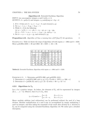
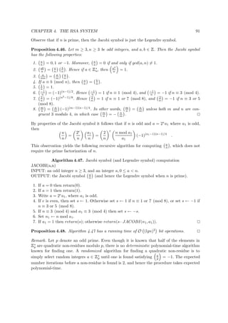
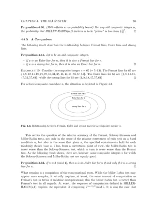
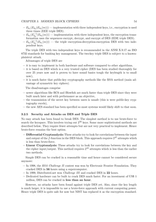
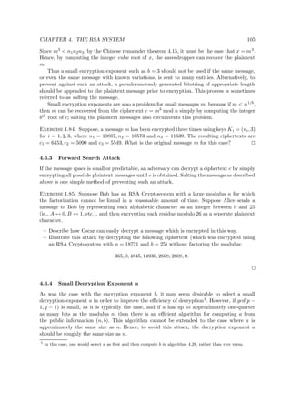
107. CHAPTER 4. THE RSA SYSTEM 101
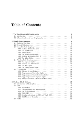
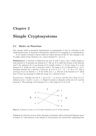
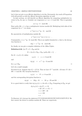
4.5.4 Elliptic curve factoring
The details of elliptic curve factoring algorithm are beyond the scope of this paper; neverthe-
less, a rough outline follows. The success of Pollard’s p − 1 algorithm hinges on p − 1 being
smooth for some prime divisor p of n; if no such p exists then the algorithm fails. Observe that
p − 1 is the order of the group
∗
p. The elliptic curve factoring algorithm is a generalization of
Pollard’s p−1 algorithm in the sense that the group
∗
p is replaced by a random elliptic curve
group over
p. The order of such a group is roughly uniformly distributed in the interval
[p + 1 − 2
√
p, p + 1 + 2
√
p]. If the order of the group chosen is smooth with respect to some
pre-selected bound, the elliptic curve algorithm will, with high probability, find a non-trivial
factor factor of n. If the group order is not smooth, then the algorithm will likely fail, but
can be repeated with a different choice of elleptic curve group.
The elleptic curve algorithm has an expected running time of Lp[1
2 ,
√
2] (the definition is
Lq[α, c] = O exp (c + o(1))(lnq)α(lnlnq)1−α ) to find a factor p of n. Since this running
time depends on the size of the prime factors of n, the algorithm tends to find small such
factors first. The elliptic curve algorithm is, therefore, classified as a special-purpose factoring
algorithm. It is currently the algorithm of choice for finding t-decimal digit prime factors, for
t ≤ 40, of very large composite integers.
In the hardest case, when n is a product of two primes of roughly the same size, the
expected running time of the elliptic curve algorithm is Ln[1
2 , 1], which is the same as that of
quadratic sieve. However, the elliptic curve algorithm is not as efficient as the quadratic sieve
in practice for such integers.
4.5.5 Quadratic sieve factoring
Suppose an integer n is to be factored. Let m =
√
n , and consider the polynomial q(x) =
(x + m)2 − n. Note that
q(x) = x2
+ 2mx + m2
− n ≈ x2
+ 2mx (4.5)
which is small (relative to n) if x is small in absolute value. The quadratic sieve algorithm
selects ai = (x + m) and tests whether bi = (x + m)2 − n is pt-smooth. Note that a2
i =
(x+m)2 ≡ bi (mod n). Note also that if a prime p divides bi then (x+m)2 ≡ n (mod p), and
hence n is quadratic residue modulo p. Thus the factor base need only contain those primes p
for which the Legendre symbol n
p is 1. Furthermore, since bi may be negative, -1 is included
in the factor base. The steps of the quadratic sieve algorithm are summarized in Algorithm
4.76.
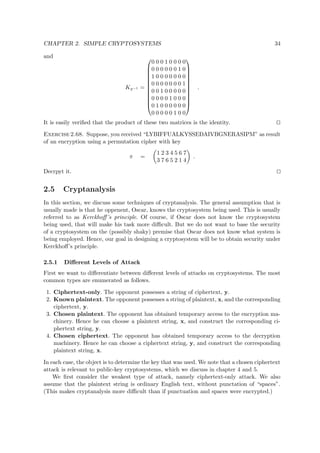
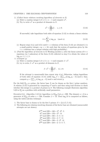
Algorithm 4.76. Quadratic sieve algorithm for factoring integers
INPUT: a composite integer n that is not a prime power.
OUTPUT: a non-trivial factor d of n.
1. Select the factor base S = {p1, . . . , pt}, where p1 = −1 and pj (j ≥ 2) is the (j − 1)th
prime p for which n is quadratic residue modulo p.
2. Compute m =
√
n .
3. (Collect t + 1 pairs (ai, bi). The x values are chosen in the order 0, ±1, ±2, . . .)
Set i ← 1. While i ≤ t + 1 do the following:

108. CHAPTER 4. THE RSA SYSTEM 102
(a) Compute b = q(x) = (x + m)2 − n, and test using trial division by elements in S
whether b is pt-smooth. If not, pick a new x and repeat step 3.1.
(b) If b is pt-smooth, say b =
t
j=1
p
eij
j , then set ai ← (x+m), bi ← b and vi = (vi1, . . . , vit),
where vij = eij mod 2 for 1 ≤ j ≤ t.
(c) i ← i + 1.
4. Use linear algebra over
2 to find a non-empty subset T ⊆ {1, 2, . . . , t + 1} such that
i∈T vi = 0.
5. Compute x = i∈T ai mod n.
6. For each j, 1 ≤ j ≤ t, compute lj = i∈T eij /2.
7. Compute y = t
j=1 p
lj
j mod n.
8. If x ≡ ±y (mod n), then find another non-empty subset T ⊆ {1, 2, . . . , t + 1} such that
i∈T vi = 0, and go to step 5. (In the unlikely case such that a subset T does not exist,
replace a few of the (ai, bi) pairs with new pairs (step 3) and go to step 4.)
9. Compute d = gcd(x − y, n) and return(d).
Example 4.22. (quadratic sieve algorithm for finding a non-trivial factor of n = 24961)
1. Select the factor base S = {−1, 2, 3, 5, 13, 23} of size t = 6. (7, 11, 17 and 19 are omitted
from S since n
p = −1 for these primes.)
2. Compute m =
√
24961 = 157.
3. Following is the data collected for the first t + 1 values of x for which q(x) is 23-smooth.
i x q(x) factorization of q(x) ai vi
1 0 −312 −23 · 3 · 13 157 (1, 1, 1, 0, 1, 0)
2 1 3 3 158 (0, 0, 1, 0, 0, 0)
3 −1 −625 −54 156 (1, 0, 0, 0, 0, 0)
4 2 320 26 · 5 159 (0, 0, 0, 1, 0, 0)
5 −2 −936 −23 · 32 · 13 155 (1, 1, 0, 0, 1, 0)
6 4 960 26 · 3 · 5 161 (0, 0, 1, 1, 0, 0)
7 −6 −2160 −24 · 33 · 5 151 (1, 0, 1, 1, 0, 0)
4. By inspection, v1 + v2 + v5 = 0. (In the notation of Algorithm 4.76, T = {1, 2, 5})
5. Compute x = a1 · a2 · a5 mod n = 936.
6. Compute l1 = 1, l2 = 3, l3 = 2, l4 = 0, l5 = 1, l6 = 0.
7. Compute y = −23 · 32 · 13 mod n = 24025.
8. Since 936 ≡ −24025 (mod n), another linear dependency must be found.
9. By inspection, v3 + v6 + v7 = 0; thus T = {3, 6, 7}.
10. Compute x = a3 · a6 · a7 mod n = 23405.
11. Compute l1 = 1, l2 = 5, l3 = 2, l4 = 3, l5 = 0, l6 = 0.
12. Compute y = −25 · 32 · 53 mod n = 13922.
13. Now, 23405 ≡ ±13922 mod n, so compute gcd(x−y, n) = gcd(9483, 24961) = 109. Hence,
two non-trivial factors of 24961 are 109 and 229.
Note 4.77. Instead of testing smoothness by trial division in step 3.1. of Algorithm 4.76, a
more efficient technique known as sieving is employed in practice. Observe first that if p is
an odd prime in the factor base and p divides q(x), then p also divides q(x + lp) for every

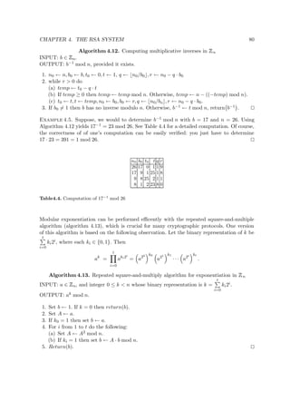
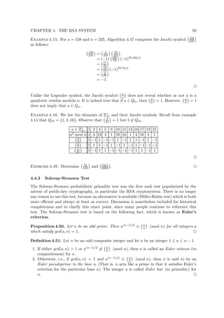
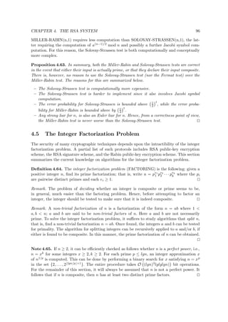
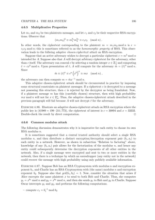
109. CHAPTER 4. THE RSA SYSTEM 103
integer l. Thus by solving the equation q(x) ≡ 0 (mod p) for x, one knows either one or two
(depending on the number of solutions to the quadratic equation) entire sequences of other
values y for which p divides q(y).
The sieving process is the following. An array Q[] indexed x, −M ≤ x ≤ M, is created and
the xth entry is initialized to lg | q(x) | . Let x1, x2 be the solutions to q(x) ≡ 0 (mod p),
where p is an odd prime in the factor base. Then the value lgp is subtracted from those
entries Q[x] in the array for which x ≡ x1 or x2 (mod p) and −M ≤ x ≤ M. This is repeated
for each odd prime p in the factor base. (The case of p = 2 and prime powers can be handled
in a similar manner.) After the sieving, the array entries Q[x] with values near 0 are most
likely to be pt-smooth (roundoff errors must be taken into account), and this can be verified
by factoring q(x) by trial division.
Note 4.78. To optimze the running time of the quadratic sieve, the size of the factor base
should be judiciously chosen. The optimal selection of t ≈ Ln[1
2 , 1
2 ] is derived from knowledge
concerning the distribution of smooth integers close to
√
n. With this choice, Algorithm 4.76
with sieving has an expected running time of Ln[1
2 , 1], independent of the size of the factors
of n.
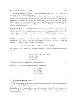
Exercise 4.79. Use the Quadratic Sieve Algorithm 4.76 to factor n = 25591.
4.6 Attacks on RSA
This section discusses various security issues related to RSA encryption. Various attacks which
have been studied in the literature are presented, as well as appropiate measures to counteract
these threats.
4.6.1 Relation to factoring
The task faced by a passive adversary is that of recovering plaintext m from the corresponding
ciphertext c, given the public information (n, b) of the intended receiver A. This is called the
RSA problem.
Definition 4.80. The RSA problem (RSAP) is the following: given a positive integer n that
is a product of two distinct odd primes p and q, a positive integer b such that gcd(b, (p −
1)(q − 1)) = 1 and an integer c, find an integer m such that mb ≡ c (mod n).
The RSAP is a computational problem whose true computational complexity is not known.
That is to say, they are widely believed to be intractible2, although no proof of this is known.
Generally, the only lower bounds known on the resources required to solve these problems
are the trivial linear bounds, which do not provide any evidence of their intractibility. It is,
therefore, of interest to study their relative difficulties. For this reason, various techniques
of reducing one computational problem to another have been devised and studied in the
literature. These reductions provide a means for converting any algorithm that solves the
second problem into an algorithm for solving the first problem. The following intuitive notion
of reducibility is used in this paper.
2
A computational problem is said to be easy or tractable if it can be solved in polynomial time, at least
for a non-negligible fraction of all possible inputs. In other words, if there is an algorithm which can solve
a non-negligible fraction of all instances of a problem in polynomial time, then any cryptosystem whose
security is based on that problem must be considered insecure.

110. CHAPTER 4. THE RSA SYSTEM 104
Definition 4.81. Let A and B be two computational problems. A is said to be polytime
reduced to B, written A ≤P B, if there is an algorithm that solves A which uses, as a
subroutine, a hypothetical algorithm for solving B, and which runs in polynomial time if the
algorithm for B does.
Informally speaking, if A polytime reduces to B, then B is at least as difficult as A; equiv-
alently, A is no harder than B. Consequently, if A is a well-studied computational problem
that is widely believed to be intractible, then proving that A ≤P B provides strong evidence
of the intractibility of problem B.
Definition 4.82. Let A and B be two computational problems. If A ≤P B and B ≤P A,
then A and B are said to be computationally equivalent, written A ≡P B.
Informally speaking, if A ≡P B then A and B are either both tractable or both intractable,
as the case may be.
One possible approach which an adversary could employ to solving the RSA problem is
to first factor n, and then compute ϕ(n) and a just as the receiver A did in Algorithm 4.28.
Once a is obtained, the adversary can decrypt any ciphertext intended for A.
On the other hand, if an adversary could somehow compute a, then it could subsequently
factor n efficiently as follows. First note that since ab ≡ 1 (mod ϕ(n)), there is an integer k
such that ab − 1 = k · ϕ(n). Hence, by Euler’s theorem, xab−1 ≡ 1 (mod n) for all x ∈
∗
n. Let
ab−1 = 2st, where t is an odd integer. Then it can be shown that there exists an i ∈ {1, . . . , s}
such that x2i−1t ≡ ±1 (mod n) and x2it ≡ 1 (mod n) for at least half of all x ∈
∗
n; if x and i
are such integers then gcd(x2i−1t −1, n) is a non-trivial factor of n. Thus the adversary simply
needs to repeatedly select random x ∈
∗
n and check if an i ∈ {1, . . . , n} satisfying the above
property exists; the expected number of trials before a non-trivial factor of n is obtained is
2. This discussion establishes following.
Proposition 4.83. The problem of computing RSA decryption exponent a from the public
key (n, b) and the problem of factoring nm are computationally equivalent.
When generating RSA keys, it is imperative that the primes p and q be selected in such a
way that factoring n = pq is computationally infeasible.
4.6.2 Small Encryption Exponent b
In order to improve the efficiency of encryption, it is desirable to select a small encryption
exponent b such as b = 3. A group of entities may all have the same encryption exponent b,
however, each entity in the group must have its own distinct modulus. If an entity A wishes
to send the same message m to three entities whose public moduli are n1, n2, n3 and whose
encryption exponents are b = 3, then A would send ci = m3 mod ni, for i = 1, 2, 3. Since these
moduli are most likely pairwise relatively prime, an eavesdropper observing c1, c2, c3 can use
Gauss’ algorithm 4.16 to find a solution x, 0 ≤ x < n1n2n3, to the three congruences



x ≡ c1 (mod n1)
x ≡ c2 (mod n2)
x ≡ c3 (mod n3).

111. CHAPTER 4. THE RSA SYSTEM 105
Since m3 < n1n2n3, by the Chinese remainder theorem 4.15, it must be the case that x = m3.
Hence, by computing the integer cube root of x, the eavesdropper can recover the plaintext
m.
Thus a small encryption exponent such as b = 3 should not be used if the same message,
or even the same message with known variations, is sent to many entities. Alternatively, to
prevent against such an attack, a pseudorandomly generated bitstring of appropriate length
should be appended to the plaintext message prior to encryption. This process is sometimes
referred to as salting the message.
Small encryption exponents are also a problem for small messages m, because if m < n1/b,
then m can be recovered from the ciphertext c = mb mod n simply by computing the integer
bth root of c; salting the plaintext messages also circumvents this problem.
Exercise 4.84. Suppose, a message m has been encrypted three times using keys Ki = (ni, 3)
for i = 1, 2, 3, where n1 = 10807, n2 = 10573 and n3 = 11639. The resulting ciphertexts are
c1 = 6453, c2 = 5090 and c3 = 5549. What is the original message m for this case?
4.6.3 Forward Search Attack
If the message space is small or predictable, an adversary can decrypt a ciphertext c by simply
encrypting all possible plaintext messages until c is obtained. Salting the message as described
above is one simple method of preventing such an attack.
Exercise 4.85. Suppose Bob has an RSA Cryptosystem with a large modulus n for which
the factorization cannot be found in a reasonable amount of time. Suppose Alice sends a
message to Bob by representing each alphabetic character as an integer between 0 and 25
(ie., A ↔ 0, B ↔ 1, etc.), and then encrypting each residue modulo 26 as a seperate plaintext
character.
– Describe how Oscar can easily decrypt a message which is encrypted in this way.
– Illustrate this attack by decrypting the following ciphertext (which was encrypted using
an RSA Cryptosystem with n = 18721 and b = 25) without factoring the modulus:
365, 0, 4845, 14930, 2608, 2608, 0.
4.6.4 Small Decryption Exponent a
As was the case with the encryption exponent b, it may seem desirable to select a small
decryption exponent a in order to improve the efficiency of decryption3. However, if gcd(p −
1, q − 1) is small, as it is typically the case, and if a has up to approximately one-quarter
as many bits as the modulus n, then there is an efficient algorithm for computing a from
the public information (n, b). This algorithm cannot be extended to the case where a is
approximately the same size as n. Hence, to avoid this attack, the decryption exponent a
should be roughly the same size as n.
3
In this case, one would select a as first and then compute b in algorithm 4.28, rather than vice versa.

112. CHAPTER 4. THE RSA SYSTEM 106
4.6.5 Multiplicative Properties
Let m1 and m2 be two plaintexts messages, and let c1 and c2 be their respective RSA encryp-
tions. Observe that
(m1m2)b
≡ mb1
1 mb2
2 ≡ c1c2 (mod n) .
In other words, the ciphertext corresponding to the plaintext m = m1m2 mod n is c =
c1c2 mod n; this is sometimes referred to as the homomorphic property of RSA. This obser-
vation leads to the follwing adaptive chosen-ciphertext attack on RSA encryption.
Suppose that an active adversary wishes to decrypt a particular ciphertext c = mb mod n
intended for A. Suppose also that A will decrypt arbitrary ciphertext for the adversary, other
than c itself. The adversary can conceal c by selecting a random integer x ∈
∗
n and computing
¯c = cxb mod n. Upon presentation of ¯c, A will compute for the adversary ¯m = (¯c)a
mod n.
Since
¯m ≡ (¯c)a
≡ ca
xb
a
≡ mx (mod n) ,
the adversary can then compute m = ¯mx−1 mod n.
This adaptive chosen-ciphertext attack should be circumvented in practice by imposing
some structural constraints on plaintext messages. If a ciphertext c is decrypted to a message
not posessing this structure, then c is rejected by the decryptor as being fraudulent. Now,
if a plaintext message m has this (carefully chosen) structure, then with high probability
mx mod n will not for x ∈
∗
n. Thus, the adaptive chosen-ciphertext attack described in the
previous paragraph will fail because A will not decrypt ¯c for the adversary.
Exercise 4.86. Illustrate an adaptive chosen-ciphertext attack on RSA encryption where the
public key is (41989 = 199 · 211, 773), the ciphertext of interest is c = 30894 and x = 33333.
Double-check the result by direct computation.
4.6.6 Common modulus attack
The following discussion demonstrates why it is imperative for each entity to choose its own
RSA modulus n.
It is sometimes suggested that a central trusted authority should select a single RSA
modulus n, and then distribute a distinct encryption/decryption exponent pair (bi, ai) to
each entity in a network. However, as shown in subsection “Relation to factoring” above,
knowledge of any (bi, ai) pair allows for the factorization of the modulus n, and hence any
entity could subsequently determine the decryption exponents of all other entities in the
network. Also, if a single message were encrypted and sent to two or more entities in the
network, then there is a technique by which an eavesdropper (any entity not in the network)
could recover the message with high probability using only publicly available information.
Exercise 4.87. Suppose Bob has an RSA Cryptosystem with modulus n and encryption ex-
ponent b1, and Charlie has an RSA Cryptosystem with (the same) modulus n and encryption
exponent b2. Suppose also that gcd(b1, b2) = 1. Now, consider the situation that arises if
Alice encrypts the same plaintext x to send to both Bob and Charlie. Thus, she computes
y1 = xb1 mod n and y2 = xb2 mod n, and then she sends y1 to Bob and y2 to Charlie. Suppose
Oscar intercepts y1 and y2, and performs the following computations.
– compute c1 = b−1
1 mod b2

113. CHAPTER 4. THE RSA SYSTEM 107
– compute c2 = c1·b1−1
b2
– compute x1 = yc1
1 · (yc2
2 )−1
mod n
1. Prove, that the value x1 is in fact Alice’s plaintext, x. Thus, Oscar can decrypt the message
Alice sent, even though the cryptosystem may be “secure”.
2. Illustrate the attack by computing x by this method if n = 18721, b1 = 43, b2 = 7717, y1 =
12677 and y2 = 14702.
4.6.7 Cycling attacks
Let c = mb mod n be a ciphertext. Let k be a positive integer such that cbk
≡ c (mod n); since
encryption is a permutation on the message space {0, 1, . . . , n − 1} such an integer k must
exist. For the same reason it must be the case that cbk−1
≡ m (mod n). This observation leads
to the following cycling attack on RSA encryption. An adversary computes cb mod n, cb2
mod
n, cb3
mod n, . . . until c is obtained for the first time. If cbk
(mod n) = c, then the previous
number in the cycle, namely cbk−1
mod n, is equal to the plaintext m.
A generalized cycling attack is to find the smallest positive integer u such that f =
gcd(cbu
− c, n) > 1. If
cbu
≡ c (mod p) and cbu
≡ c (mod q) (4.6)
then f = p. Similarily, if
cbu
≡ c (mod p) and cbu
≡ c (mod q) (4.7)
then f = q. In either case, n has been factored, and the adversary can recover a and then m.
On the other hand, if both
cbu
≡ c (mod p) and cbu
≡ c (mod q), (4.8)
then f = n and cbu
≡ c (mod n). In fact, u must be the smallest positive integer k for which
cbk
≡ c (mod n). In this case, the basic cycling attack has succeeded and so m = cbu−1
mod n
can be computed efficiently. Since (4.8) is expected to occur much less frequently than (4.6)
and (4.7), the generalized cycling attack usually terminates before the cycling attack does.
For this reason, the generalized cycling attack can be viewed as being essentially an algorithm
for factoring n.
Since factoring n is assumed to be intractible, these cycling attacks do not pose a threat
to the security of RSA encryption.
Exercise 4.88. Assume the ciphertext c = 216 has been encrypted using RSA with the key
K = (221, 5). Determine the plaintext p belonging to c with a cycling attack and without
factoring 221 or determining a. How long does it take when using the general approach?
4.6.8 Message Concealing
A plaintext message m, 0 ≤ m ≤ n − 1 in the RSA public-key encryption scheme is said to be
unconcealed if it encrypts to itself; that is, mb ≡ m (mod n). There are always some messages

114. CHAPTER 4. THE RSA SYSTEM 108
which are unconcealed (for example m = 0, m = 1 and m = n − 1). In fact, the number of
unconcealed messages is exactly
(1 + gcd(b − 1, p − 1)) · (1 + gcd(b − 1, q − 1)) .
Since b−1, p−1 and q −1 are all even, the number of unconcealed messages is always at least
9. If p and q are random primes, and if b is chosen at random (or if b is chosen to be a small
number such as b = 3 or b = 216 + 1 = 65537), then the proportion of messages which are
unconcealed by RSA encryption will, in general, be negligibly small, and hence unconcealed
messages do not pose a threat to the security of RSA encryption in practice.
4.7 RSA Encryption in Practice
There are numerous ways of speeding up RSA encryption and decryption in software and
hardware implementations. Some of these techniques include fast modular multiplication,
fast modular exponentiation and the use of the Chinese remainder theorem for faster de-
cryption. Even with these improvements, RSA encryption/decryption is substantially slower
than the commonly used symmetric-key encryption algorithm such as DES. In practice, RSA
encryption is most commonly used for the transport of symmetric-key encryption algorithm
keys and for the encryption of small items.
The RSA cryptosystem has been patented in the U.S. and Canada. Several standards
organizations have written, or are in the process of writing, standards that address the use of
the RSA cryptosystem for encryption, digital signatures, and key establishment.
Note 4.89. (recommended size of the modulus) Given the latest progress in algorithms for
factoring integers, a 512-bit modulus n provides only marginal security from concerted attack.
As of 1996, in order to foil the powerful quadratic sieve and number field sieve factoring
algorithms, a modulus n of at least 768 bits is recommended. For long-term security, 1024-bit
or larger moduli should be used.
Note 4.90. (selecting primes)
1. The primes p and q should be selected so that factoring n = pq is computationally
infeasible. The major restriction to p and q in order to avoid the elliptic curve factoring
algorithm is that p and q should be about the same bitlength, and sufficently large. For
example, if a 1024-bit modulus n is to be used, then each of p and q should be about 512
bits in length.
2. Another restriction on the primes p and q is that the difference p − q should not be too
small. If p − q is small, then p ≈ q and hence p ≈
√
n. Thus, n could be factored efficently
simply by trial division by all odd integers close to
√
n. If p and q are chosen at random,
then p − q will be appropriately large with overwhelming probability.
3. In addition to these restrictions, many authors have recommended that p and q be strong
primes. A prime p is said to be strong prime iff the following three conditions are satisfied:
(a) p − 1 has a large prime factor, denoted r;
(b) p + 1 has a large prime factor; and
(c) r − 1 has a large prime factor.

115. CHAPTER 4. THE RSA SYSTEM 109
There are algorithms for generating strong primes. The reason for condition (a) is to foil
Pollard’s p − 1 factoring algorithm which is efficient only if n has a prime factor p such
that p − 1 is smooth. Condition (b) foils the p + 1 factoring algorithm, which is efficient
only if n has a prime factor p such that p + 1 is smooth. Finally, condition (c) ensures
that the cycling attacks will fail.
If the prime p is randomly chosen and is sufficently large, then both p − 1 and p + 1 can
be expected to have large prime factors. In any case, while strong primes protect against
the p − 1 and p + 1 factoring algorithms, they do not protect against their generalization,
the elliptic curve factoring algorithm. The latter is successful in factoring n if a randomly
chosen number of the same size as p (more precisely, this number is the order of a randomly
selected elliptic curve defined over
p) has only small prime factors. Additionally, it has
been shown that the chances of a cycling attack succeeding are negligible if p and q
are randomly chosen. Thus, strong primes offer little protection beyond that offered by
random primes. Given the current state of knowledge of factoring algorithms, there is
no compelling reason for requiring the use of strong primes in RSA key generation. On
the other hand, they are no less secure than random primes, and require only minimal
additional running time to compute; thus there is little real additional cost in using them.
Note 4.91. (small encryption exponents)
1. If the encryption exponent b is chosen at random, then RSA encryption using the repeated
square-and-multiply algorithm 4.13 takes k modular squarings and an expected k/2 (less
with optimizations) modular multiplications, where k is the bitlength of the modulus n.
Encryption can be sped up by selecting b to be small and/or by selecting b with a small
number of 1’s in it’s binary representation.
2. The encryption exponent b = 3 is commonly used in practice; in this case, it is necessary
that neither p−1 nor q−1 be divisible by 3. This results in a very fast encryption operation
since encryption only requires 1 modular multiplication and 1 modular squaring. Another
encryption exponent used in practice is b = 216 + 1 = 65537. This number has only
two 1’s in its binary representation, and so encryption using the repeated square-and-
multiply algorithm requires only 16 modular squarings and 1 modular multiplication.
The encryption exponent b = 216 + 1 has the advantage over b = 3 in that it resists the
kind of attack discussed in subsection 4.6.2, since it is unlikely the same message will be
sent to 216 + 1 recipients.

116. Chapter 5
The ElGamal Cryptosystem
In this chapter, we look at a different public-key cryptosystem. The ElGamal Cryptosystem
is based on the Discrete Logarithm problem, which plays an important role in numerous cryp-
tographic protocols in practice. Thus we devote a considerable amount of time to discussion
of this important problem.
5.1 The ElGamal Cryptosystem and Discrete Logarithms
The ElGamal Cryptosystem is based on the Discrete Logarithm problem. We begin by de-
scribing this problem in the setting of a finite field
p, where p is prime. Recall that the
multiplicative group
∗
p is cyclic, and a generator of
∗
p is called a primitive element.
Definition 5.1. The discrete logarithm problem is the following: given a prime p, a generator
α of
∗
p, and an element β ∈
∗
p, find the integer a, 0 ≤ a ≤ p − 2, such that αa ≡ β (mod p).
The integer a is denoted by logα β and called the discrete logarithm of β to the base α.
Example 5.1. Let p = 97. Then
∗
97 is a cyclic group of order n = 96. A generator of
∗
97 is
α = 5. Since 532 ≡ 35 (mod 97), log5 35 = 32 in
∗
97.
There is no reason to restrict ourselves to the cyclic group
p. Instead of this we can generalize
the problem to an arbitrary finite cyclic group.
Definition 5.2. The generalized discrete logarithm problem is the following: given a finite
cyclic group G of order n, a generator α of G, and an element β ∈ G, find the integer
a, 0 ≤ a ≤ n − 1, such that αa ≡ β (mod n). Again, a is called the discrete logarithm of β to
the base α.
Here are some simple facts about discrete logarithms.
Proposition 5.3. Let α be a generator of a cyclic group G of order n, and let β, γ ∈ G. Let s
be an integer. Then logα(βγ) = (logα β + logα γ) mod n and logα (βs) = s logα β mod n.
Note 5.4. (difficulty of the generalized discrete logarithm problem is independent of gen-
erator) Let α and γ be two generators of a cyclic group G of order n, and let β ∈ G.
Let x = logα β, y = logγ β and z = logα γ. Then αx = β = γy = (αz)y
. Consequently
x = zy mod n and
logγ β = (logα β) (logα γ)−1
mod n .

117. CHAPTER 5. THE ELGAMAL CRYPTOSYSTEM 111
This means that any algorithm which computes logarithms to the base α can be used to
compute logarithms to any other base γ that is also a generator of G.
The Discrete Logarithm problem in
p has been the object of much study. The problem is
generally regarded as being difficult if p is carefully chosen. In particular, there is no known
polynomial-time algorithm for the Discrete Logarithm problem. To thwart known attacks, p
should have at least 150 digits, and p − 1 should have at least one “large” prime factor. The
utility of the Discrete Logarithm problem in a cryptographic setting is that finding discrete
logs is (probably) difficult, but the inverse operation of exponentiation can be computed effi-
ciently by using the square-and-multiply algorithm 4.13. Stated another way, exponentiation
modulo p is a one-way function for suitable primes p.
ElGamal has developed a public-key cryptosystem based on the Discrete Logarithm prob-
lem. This system is presented now.
Definition 5.5. Let p be a prime such that the discrete log problem in
p is intractable, and
let α ∈
∗
p be a primitive element. Let P =
∗
p and C =
∗
p ×
∗
p, and define
K = {(p, α, a, β) | β ≡ αa
(mod p)} .
The values p, α and β are public, and a is secret. For K = (p, α, a, β) and for a (secret) random
number k ∈
p−1, define
eK(x, k) = (y1, y2) ,
where
y1 = αk
mod p
and
y2 = xβk
mod p .
For y1, y2 ∈
∗
p, define
dK (y1, y2) = y2 (ya
1)−1
mod p.
The ElGamal Cryptosystem is non-deterministic, since the ciphertext depends on both the
plaintext x and on the random value k chosen by Alice. So there will be many ciphertexts
that are encryptions of the same plaintext.
Informally, this is how the ElGamal Cryptosystem works. The plaintext x is “masked” by
multiplying it by βk, yielding y2. The value αk is also transmitted as part of the ciphertext.
Bob, who knows the secret exponent a, can compute βk from αk. Then he can “remove the
mask” by dividing y2 by βk to obtain x.
Algorithm 5.6. Key generation for ElGamal public-key encryption
SUMMARY: each entity creates a public key and a corresponding private key.
Each entity A should do the following.
1. Generate a large random prime p and a generator α of the multiplicative group
∗
p of the
integers modulo p.
2. Select a random integer a, 1 ≤ a ≤ p − 2 and compute αa mod p (using Algorithm 4.13).
3. A’s public key is (p, α, αa); A’s private key is a.

118. CHAPTER 5. THE ELGAMAL CRYPTOSYSTEM 112
Algorithm 5.7. ElGamal public-key encryption
SUMMARY: B encrypts a message x for A, which A decrypts
1. Encryption. B should do the following:
(a) Obtain A’s authentic public key p, α, αk .
(b) Represent the message as an integer x in the range {0, 1, . . . , p − 1}.
(c) Select a random integer k, 1 ≤ k ≤ p − 2.
(d) Compute y1 = αk mod p and y2 = x · (αa)k
mod p.
(e) Send the ciphertext c = (y1, y2) to A.
2. Decryption. To recover plaintext x from c, A should do the following.
(a) Use the private key a to compute ya
1 mod p.
(b) Recover x by computing y2 · (ya
1)−1
mod p.
The decryption of Algorithm 5.7 allows recovery of the original plaintext because
y2 (ya
1 )−1
≡ xβk
αka
−1
≡ xβk
(αa
)k
−1
≡ xβk
βk
−1
≡ x (mod p).
Example 5.2. ElGamal encryption with artificially small parameters.
Key generation. Entity A selects the prime p = 2357 and a generator α = 2 of
∗
2357. A
chooses the private key a = 1751 and computes
αa
mod p = 21751
mod 2357 = 1185.
A’s public key is (p = 2357, α = 2, αa = 1185).
Encryption. To encrypt a message x = 2035, B selects a random integer k = 1520 and
computes
y1 = 21520
mod 2357 = 1430
and
y2 = 2035 · 11851520
mod 2357 = 697.
B sends (y1 = 1430, y2 = 697) to A.
Decryption. To decrypt, A computes
ya
1 = 14301751
mod 2357 = 1760,
and recovers x by computing
x = 697 · 1760−1
mod 2357 = 697 · 872 mod 2375 = 2035.
Note 5.8. (common system-wide parameters) All entities may elect to use the same prime p
and generator α, in which case p and α need not be published as part of the public key. This
results in public keys of smaller sizes. An additional advantage of having a fixed base α is
that exponentiation can then be expedited via precomputations. A potential disadvantage of
common system-wide parameters is that larger moduli p may be warranted.
Note 5.9. (efficiency of ElGamal encryption)

119. CHAPTER 5. THE ELGAMAL CRYPTOSYSTEM 113
– The encryption process requires two modular exponentiations, namely αk mod p and
(αa)k
mod p. These exponentiations can be sped up by selecting random exponents k
having some additional structure, for example, having low Hamming weights (,i.e., the
number of 1 in their binary representations is low). Care must be taken that the possi-
ble number of exponents is large enough to preclude a search via a baby-step giant-step
algorithm.
– A disadvantage of ElGamal encryption is that there is message expansion by a factor of
2. That is, the ciphertext is twice as long as the corresponding plaintext.
Note 5.10. (recommended parameter size) Given the last progress on the discrete logarithm
problem in
∗
p, a 512-bit modulus p provides only marginal security from concerted attack.
As of 1996, a modulus p of at least 768 bits is recommended. For long-term security, 1024-
bit or larger moduli should be used. For common system-wide parameters even larger key
sizes may be warranted. This is because the dominant stage in the index-calculus algorithm
for discrete logarithms in
∗
p is the precomputation of a database of factor base logarithms,
following which individual logarithms can be computed relatively quickly. Thus computing
the database of logarithms for one particular modulus p will compromise the secrecy of all
private keys derived using p.
5.2 Algorithms for the Discrete Log Problem
In this section we will present various algorithms for the generalized discrete logarithm prob-
lem. The most obvious method is to successively compute α0, α1, α2, . . . until β is obtained.
This method, called exhaustive search, takes O(n) multiplications, where n is the order of α
and is therefore inefficient if n is large (,i.e., in cases of cryptographic interest).
5.2.1 The Baby-Step-Giant-Step Algorithm
Let m =
√
n , where n is the order of α. The baby-step giant-step algorithm is a time-memory
trade-off of the method of exhaustive search and is based on the following observation. If
β = αx, then one can write x = im + j, where 0 ≤ i, j, < m. Hence, αx = αimαj, which
implies β(α−m)i = aj. This suggests the following algorithm for computing x.
Algorithm 5.11. Baby-step giant-step algorithm for computing discrete logarithms
INPUT: a generator α of a cyclic group G of order n, and an element β ∈ G.
OUTPUT: the discrete logarithm x = logα β.
1. Set m ←
√
n .
2. Construct a table with entries (j, αj) for 0 ≤ j < m. Sort this table by second component.
3. Compute α−m and set γ ← β.
4. For i from 0 to m − 1 do the following:
(a) Check if γ is the second component of some entry in the table.
(b) If γ = αj then return(x = im + j).
(c) Set γ ← γ · α−m.
Algorithm 5.11 requires storage for O(
√
n) group elements. The table takes O(
√
n) multi-
plications to construct, and O(
√
n lg n) comparisons to sort. Having constructed this table,
step 4 takes O(
√
n) multiplications and O(
√
n) table look-ups. Under the assumption that a

120. CHAPTER 5. THE ELGAMAL CRYPTOSYSTEM 114
group multiplication takes more time than lg n comparisons, the running time of Algorithm
5.11 can be stated more concisely as follows.
Proposition 5.12. The running time of the baby-step giant-step Algorithm 5.11 is O(
√
n)
group multiplications.
Example 5.3. (baby-step giant-step algorithm for logarithms in
∗
113). Let p = 113. The
element α = 3 is a generator of
∗
113 of order n = 112. Consider β = 57. Then log3 57 is
computed as follows.
1. Set m ←
√
n = 11.
2. Construct a table whose entries are (j, αj mod p) for 0 ≤ j < 11:
j 0 1 2 3 4 5 6 7 8 9 10
3j (mod 113) 1 3 9 27 81 17 51 40 7 21 63
and sort the table by second component:
j 0 1 8 2 5 9 3 7 6 10 4
3j (mod 113) 1 3 7 9 17 21 27 40 51 63 81
3. Using Algorithm 4.12, compute α−1 = 3−1 mod 113 = 38 and then compute α−m =
3811 mod 113 = 58.
4. Next, γ = βα−mi mod 113 for i = 0, 1, 2, . . . is computed until a value in the second row
of the table is obtained. This yields:
j 0 1 2 3 4 5 6 7 8 9
γ = 57 · 58i (mod 113) 57 29 100 37 112 55 26 39 2 3
Finally, since βα−9m = 3 = α1, β = α100 and therefore, log3 57 = 100.
Exercise 5.13. Let p = 643. A generator of
∗
643 is α = 11. Considering β = 315, compute
log11 315.
5.2.2 Pollard’s ρ-algorithm for Discrete Logs
Pollard’s ρ algorithm for computing discrete logarithms is a randomized algorithm with the
same expected running time as the baby-step giant-step algorithm, but which requires a
negligible amount of storage. For this reason, it is far preferable to Algorithm 5.11 for problems
of practical interest. For simplicity, it is assumed in this subsection that G is a cyclic group
whose order n is prime.
The group G is partitioned into three sets S1, S2 and S3 of roughly equal size based on
some easily testable property. Some care must be exercised in selecting the partition; for
example 1 /∈ S2. Define a sequence of group elements x0, x1, x2, . . . by x0 = 1 and
xi+1 = f(xi) =



β · xi, if xi ∈ S1,
x2
i , if xi ∈ S2,
α · xi, if xi ∈ S3,
(5.9)

121. CHAPTER 5. THE ELGAMAL CRYPTOSYSTEM 115
for i ≥ 0. This sequence of group elements in turn defines sequences of integers a0, a1, a2, . . .
and b0, b1, b2, . . . satisfying xi = αai βbi for i ≥ 0: a0 = 0, b0 = 0 and for i ≥ 0:
ai+1 =



ai, if xi ∈ S1,
2ai mod n, if xi ∈ S2,
ai + 1 mod n, if xi ∈ S3,
(5.10)
and
bi+1 =



bi + 1 mod n, if xi ∈ S1,
2bi mod n, if xi ∈ S2,
bi, if xi ∈ S3.
(5.11)
Floyd’s cycle-finding Algorithm 4.67 can then be utilized to find two group elements xi and
x2i such that xi = x2i. Hence αai βbi = αa2i βb2i and so βbi−b2i = αa2i−ai . Taking logarithms
to the base α of both sides of this last equation yields
(bi − b2i) · logα β ≡ (a2i − ai) (mod n).
Provided bi ≡ b2i (mod n) (note: bi ≡ b2i occurs with negligible property), this equation can
then be efficiently solved to determine logα β.
Algorithm 5.14. Pollard’s ρ algorithm for computing discrete logarithms
INPUT: a generator α of a cyclic group G of prime order n, and an element β ∈ G.
OUTPUT: the discrete logarithm logα β.
1. Set x0 ← 1, a0 ← 0, b0 ← 0.
2. For i = 1, 2, . . . do the following:
(a) Using the quantities xi−1, ai−1, bi−1 and x2i−2, a2i−2, b2i−2 computed previously, com-
pute xi, ai, bi and x2i, a2i, b2i using equations (5.9), (5.10) and (5.11).
(b) If xi = x2i, then do the following:
Set r ← bi − b2i (mod n).
If r = 0 then terminate the algorithm with failure; otherwise,
compute x = r−1(a2i − ai) mod n and return(x).
In the rare case that Algorithm 5.14 terminates with failure, the procedure can be repeated
by selecting random integers a0, b0 ∈ {1, . . . , n − 1} and starting with x0 = αa0 βb0 .
Example 5.4. (Pollard’s ρ algorithm for logarithms in a subgroup of
∗
383) The element α = 2
is a generator of the subgroup G of
∗
383 of order n = 191. Suppose β = 228. Partition the
elements of G into three subsets according to the rule x ∈ S1 if x ≡ 1 (mod 3), x ∈ S2 if x ≡ 0
(mod 3) and x ∈ S3 if x ≡ 2 (mod 3). Table 5.1 shows the values of xi, ai, bi, x2i, a2i and b2i at
the end of each iteration step of algorithm 5.14. Note that x14 = x28 = 144. Finally, compute
r = b14 − b28 mod 191 = 125, r−1 = 125−1 mod 191 = 136 and r−1(a28 − a14) mod 191 = 110.
Hence, log2 228 = 110.
Proposition 5.15. Let G be a group of order n, a prime. Assume that the function f : G → G
defined by equation (5.10) behaves like a random function. Then the expected running time of
Pollard’s ρ algorithm for discrete logarithms in G is O (
√
n) group operations. Moreover, the
algorithms requires negligible storage.

122. CHAPTER 5. THE ELGAMAL CRYPTOSYSTEM 116
i xi ai bi x2i a2i b2i
1 228 0 1 279 0 2
2 279 0 2 184 1 4
3 92 0 4 14 1 6
4 184 1 4 256 2 7
5 205 1 5 304 3 8
6 14 1 6 121 6 18
7 28 2 6 144 12 38
8 256 2 7 235 48 152
9 152 2 8 72 48 154
10 304 3 8 14 96 118
11 372 3 9 256 97 119
12 121 6 18 304 98 120
13 12 6 19 121 5 51
14 144 12 38 144 10 104
Table5.1. Intermediate steps of Pollard’s ρ algorithm in example 5.4
Exercise 5.16. 1. Consider the cyclic group
∗
311. Then α = 17 is a generator for this group.
Take β = 67 and apply Pollards ρ Algorithm 5.14 to compute logα β. Check your result
by verifying the equation αlogα β = β. What went wrong?
2. Consider the subgroup G of
∗
79 that is generated by α = 67 and has order n = 13. Use
Pollard’s ρ Algorithm 5.14 to compute logα β, verify your result, determine all elements
of G and double- check again.
5.2.3 The Pohlig-Hellman Algorithm
Algorithm 5.17 for computing logarithms takes advantage of the factorization of the order n
of the group G. Let n = pe1
1 pe2
2 · · · per
r be the prime factorization of n. If x = logα β, then the
approach is to determine xi = x mod pei
i for 1 ≤ i ≤ r, and then use Gauss’s algorithm 4.16
to recover x mod n. Each integer xi is determined by computing the digits l0, l1, . . . , lei−1 in
turn of its pi-ary representation: xi = l0 + l1pi + . . . + lei−1pei−1
i , where 0 ≤ lj ≤ pi − 1.
To see that the algorithm 5.17 is correct, observe first that in step 2.c) the order of ¯α is
q. Next, at iteration j of step 2.d), γ = αl0+l1q+...+lj−1qj−1
. Hence,
¯β = (β/γ)n/qj+1
= αx−l0−l1q−...−lj−1qj−1 n/qj+1
= αn/qj+1 xi−l0−l1q−...−lj−1qj−1
= αn/qj+1 ljqj +...+le−1qe−1
= αn/q
lj +...+le−1qe−1−j
= (¯α)lj
,
the last equality being true because ¯α has order q. Hence, log ¯α
¯β is indeed equal to lj.

123. CHAPTER 5. THE ELGAMAL CRYPTOSYSTEM 117
Algorithm 5.17. Pohlig-Hellman algorithm for computing discrete logarithms
INPUT: a generator α of a cyclic group G of order n, and an element β ∈ G
OUTPUT: the discrete logarithm x = logα β.
1. Find the prime factorization of n: n = pe1
1 pe2
2 · · · per
r , where ei ≥ 1.
2. For i from 1 to r do the following:
(Compute xi = l0 + l1pi + . . . + lei−1pei−1
i , where xi = x mod pei
i )
(a) (Simplify the notation) Set q ← pi and e ← ei.
(b) Set γ ← 1 and l−1 ← 0.
(c) Compute ¯α ← αn/q.
(d) (Compute the lj) For j from 0 to e − 1 do the following:
Compute γ ← γαlj−1qj−1
and ¯β ← βγ−1 n/qj+1
.
Compute lj ← log¯α
¯β (,e.g., using Algorithm 5.11)
(e) Set xi ← l0 + l1q + . . . + le−1qe−1.
3. Use Gauss’s Algorithm 4.16 to compute the integer x, 0 ≤ x ≤ n − 1, such that x ≡ xi
(mod pei
i ) for 1 ≤ i ≤ r.
4. Return(x).
The next example illustrates Algorithm 5.17 with artificially small parameters.
Example 5.5. (Pohig-Hellman algorithm for logarithms in
∗
251) Let p = 251. The element
α = 71 is a generator of
∗
251 of order n = 250. Consider β = 210. Then x = log71 210 is
computed as follows.
1. The prime factorization of n is 250 = 2 · 53.
2. (a) (Compute x1 = x mod 2)
Compute ¯α = αn/2 mod p = 250 and ¯β = βn/2 mod p = 250. Then x1 = log250 250 =
1.
(b) (Compute x2 = x mod 53 = l0 + l15 + l252)
i. Compute ¯α = αn/5 mod p = 20.
ii. Compute γ = 1 and ¯β = βγ−1 n/5
mod p = 149. Using exhaustive search1,
compute l0 = log20 149 = 2.
iii. Compute γ = γα2 mod p = 21 and ¯β = βγ−1 (p−1)/125
mod p = 113. Using
exhaustive search, compute l1 = log20 113 = 4.
iv. Compute γ = γα4·5 mod p = 115 and ¯β = βγ−1 (p−1)/125
mod p = 149. Using
exhaustive search, compute l2 = log20 149 = 2.
Hence, x2 = 2 + 4 · 5 + 2 · 52 = 72.
3. Finally, solve the pair of congruences x ≡ 1 (mod 2), x ≡ 72 (mod 125) to get x =
log71 210 = 197.
Proposition 5.18. Given the factorization of n, the running time of the Pohlig-Hellman
Algorithm 5.17 is O r
i=1 ei(lg n +
√
pi) group multiplications.
Note 5.19. (effectiveness) Proposition 5.18 implies that the Pohlig-Hellman algorithm is ef-
ficient only if each prime divisor pi of n is relatively small; that is, if n is a smooth integer.
1
Exhaustive search is preferable to Algorithm 5.11 when the group is very small (here the order of ¯α is 5)

124. CHAPTER 5. THE ELGAMAL CRYPTOSYSTEM 118
An example of a group in which the Pohlig-Hellman algorithm is effective follows. Consider
the multiplicative group
∗
p where p is the 107-digit-prime:
p = 227088231986781039743145181950291021585250524967592855
96453269189798311427475159776411276642277139650833937.
The order of
∗
p is n = p − 1 = 24 · 1047298 · 2247378 · 3503774. Since the largest prime divisor
of p − 1 is only 350377, it is relatively easy to compute logarithms in this group using the
Pohlig-Hellman algorithm.
Note 5.20. (miscellaneous)
– If n is a prime, then algorithm 5.17 is the same as baby-step giant-step Algorithm 5.11.
– In step 1 of Algorithm 5.17, a factoring algorithm which finds small factors first (,e.g.,
Algorithm 4.72) should be employed; if the order n is not a smooth integer, then Algorithm
5.17 is inefficient anyway.
– The storage required for Algorithm 5.11 in step 2.(d) can be eliminated by using instead
Pollard’s ρ Algorithm 5.14.
Exercise 5.21. α = 17 is a generator of
∗
311 that has group order n = 310. Assume β = 67.
Compute log17 67 using the Pohlig-Hellman Algorithm 5.17.
5.2.4 The Index Calculus Method
The index-calculus algorithm is the most powerful method known for computing discrete
logarithms. The technique employed does not apply to all groups, but when it does, it often
gives a subexponential-time algorithm. The algorithm is first described in the general setting
of a cyclic group G (Algorithm 5.22). One example is then presented to illustrate how the
index-calculus algorithm works in kind of groups that are used in practical applications,
namely
∗
p.
The index-calculus algorithm requires the selection of a relatively small subset S of ele-
ments of G, called the factor base, in such a way that a significant fraction of elements of G
can be efficiently expressed as products of elements in S, and then reuses this database each
time the logarithm of a particular group element is required.
The description of algorithm 5.22 is incomplete for two reasons. Firstly, a technique for
selecting the factor base S is not specified. Secondly, a method for efficiently generating
relations of the form (5.12) and (5.14) is not specified. The factor base S must be a subset of
G that is small (so that the system of equations to be solved in step 3 is not too large), but
not too small (so that the expected number of trials to generate a relation (5.12) or (5.14)
is not too large). Suitable factor bases and techniques for generating relations are known for
some cyclic subgroups including
∗
p.
Algorithm 5.22. Index-calculus algorithm for discrete logarithms in cyclic groups
INPUT: a generator α of a cyclic group G of order n and an element β ∈ G
OUTPUT: the discrete logarithm y = logα β.
1. (Select a factor base S) Choose a subset S = {p1, p2, . . . , pt} of G such that a “significant
proportion” of all elements in G can be efficiently expressed as a product of elements from
S.

125. CHAPTER 5. THE ELGAMAL CRYPTOSYSTEM 119
2. (Collect linear relations involving logarithms of elements in S)
(a) Select a random integer k, 0 ≤ k ≤ n − 1 and compute αk.
(b) Try to write αk as a product of elements in S:
αk
=
t
i=1
pei
i , ci ≥ 0. (5.12)
If successful, take logarithms both sides of equation (5.12) to obtain a linear relation
k ≡
t
i=1
ei logα pi (mod n). (5.13)
(c) Repeat steps 2.(a) and 2.(b) until t + c relations of the form (5.13) are obtained (c is
a small positive integer, e.g. c = 10, such that the system of equations given by the
t + c relations has a unique solution with high probability).
3. (Find the logarithms of elements in S) Working modulo n, solve the linear system of t+c
equations (in t unknowns) of the form (5.13) collected in step 2 to obtain the values of
logα pi, 1 ≤ i ≤ t.
4. (Compute y)
(a) Select a random integer k, 0 ≤ k ≤ n − 1 and compute β · αk.
(b) try to write β · αk as a product of elements in S:
β · αk
=
t
i=1
pdi
i , di ≥ 0. (5.14)
If the attempt is unsuccessful then repeat step 4.(a). Otherwise, taking logarithms
of both sides of equation (5.14) yields logα β = t
i=1 di logα pi − k mod n; thus,
compute y = t
i=1 di logα pi − k mod n and return y.
For the field
p, p a prime, the factor base S can be chosen as the first t prime numbers.
A relation (5.12) is generated by computing αk mod n and then using trial division to check
whether this integer is a product of primes in S. The following example illustrates algorithm
5.22 in
∗
p on a problem with artificially small parameters.
Example 5.6. (Algorithm 5.22 for logarithms in
∗
229) Let p = 229. The element α = 6 is a
generator of
∗
229 of order n = 228. Consider β = 13. Then log6 13 is computed as follows,
using the index-calculus technique.
1. The factor base is chosen to be the first 5 primes: S = {2, 3, 5, 7, 11}.
2. The following six relations involving elements of the factor base are obtained (unsuccessful
attempts are not shown):
6100 mod 229 = 180 = 22 · 32 · 5
618 mod 229 = 176 = 24 · 11
612 mod 229 = 165 = 3 · 5 · 11
662 mod 229 = 154 = 2 · 7 · 11
6143 mod 229 = 198 = 2 · 32 · 11
6206 mod 229 = 210 = 2 · 3 · 5 · 7.

126. CHAPTER 5. THE ELGAMAL CRYPTOSYSTEM 120
These relations yield the following six equations involving the logarithms of elements in
the factor base:
100 ≡ 2 log6 2 + 2 log6 3 + log6 5 (mod 228)
18 ≡ 4 log6 2 + log6 11 (mod 228)
12 ≡ log6 3 + log6 5 + log6 11 (mod 228)
62 ≡ log6 2 + log6 7 + log6 11 (mod 228)
143 ≡ log6 2 + 2 log6 3 + log6 11 (mod 228)
206 ≡ log6 2 + log6 3 + log6 5 + log6 7 (mod 228).
3. Solving the linear system of six equations in five unknowns (the logarithms xi = log6 pi)
yields the solutions log6 2 = 21, log6 3 = 208, log6 5 = 98, log6 7 = 107 and log6 11 = 162.
4. Suppose that the integer k = 77 is selected. Since β · αk = 13 · 677 mod 229 = 147 = 3 · 72,
it follows that
log6 13 = (log6 3 + 2 log6 7 − 77) mod 228 = 117.

127. Chapter A
Cryptography Timeline
This chapter has been added to give an impression in what kind of areas cryptography has
played an important role. We start with a quotation of David Kahn’s “The Codebreakers”:
“It must be that as soon as a culture has reached a certain level, probably measured largely
by its literacy, cryptography appears spontaneously—as its parents, language and writing,
probably also did. The multiple human needs and desires that demand privacy among two or
more people in the midst of social life must inevitably lead to cryptology wherever men thrive
and wherever they write. Cultural diffusion seems a less likely explanation for its occurence
in so many areas, many of them distant and isolated.”
The invention of cryptography is not limited to either civilians or the government. Wher-
ever the need for secrecy is felt, the invention occurs. However, over time the quality of the
best available system continues to improve and those best systems were often invented by
civilians. Again, from David Kahn:
“It was the amateurs of cryptology who created the species. The professionals, who almost
certainly surpassed them in cryptanalytic expertise, concentrated on down-to-earth problems
of the system that were then in use but are now outdated. The amateurs, unfettered to those
realities, soared into the empyrean of theory.”
In the table to follow, each descyption starts with (date; civ or govt; source). Sources are
identified in full at the end.
Date C or G Source Info
about 1900 BC civ Kahn, p.71 An Egyptian scribe used non-standard hieroglyphs
in an inscription. Kahn lists this at the first
document example of written cryptography.
1500 BC civ Kahn, p.75 A Mesopotamian tablet contains an enciphered
formula for the making of glazes for pottery.
600-500 BC civ Kahn, p.77 Hebrew scribes writing down the book of
Jeremiah used a reversed-alphabet simple
substitution cipher known as ATBASH.
Jeremiah started dictating to Baruch in 605
BC but the chapters containing these bits
of cipher are attributed to a source labeled
“C” (believed not to be Baruch) which could

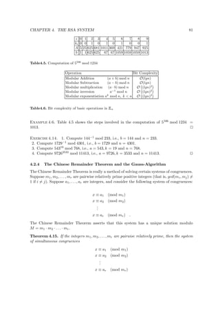
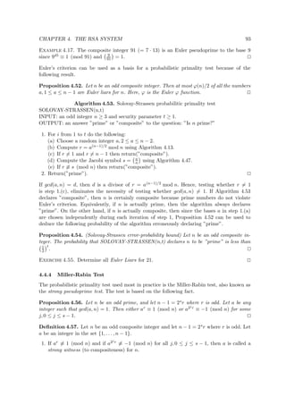
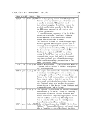
128. CHAPTER A. CRYPTOGRAPHY TIMELINE 122
Date C or G Source Info
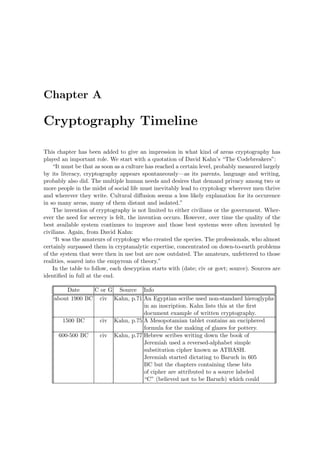
be an editor writing after Babylonian exile
in 587 BC, someone contemporaneous with
Baruch or even Jeremiah himself. ATBASH was
one of a few Hebrew ciphers of the time.
487 BC govt Kahn, p.82 The greeks used a device called the
“skytale”—a staff around which a long,
thin strip of leather was wrapped and written
on. The leather was taken off and worn as a
belt. Presumably, the recipient would have a
matching staff and the encryption staff would
be left at home.
60-50 BC govt Kahn, p.83 Julius Caesar (100-44 BC) used a simple substitution
with the normal alphabet (just shifting the letters a
fixed amount) in government communications. This
cipher was less strong than ATBASH, by a small
amount, but in a day when people read in the first
place, it was good enough. He also used
transliteration of Latin into Greek letters and a
number of other simple ciphers.
0-400? civ Burton The Kama Sutra of Vatsayana lists cryptography
as the 44th and 45th of 64 arts (yogas) men and
women should know and practice. The date of this
work is unclear but is believed to be between
the first and fourth centuries, AD. Vatsayana
says that his Kama Sutra is a compilation of
much earlier works, making the dating of the
cryptography references even more uncertain.
Part I, Chapter III lists the 64 arts and opens
with: “Man should study the Kama Sutra and the
arts and sciences subordinate thereto[...] Even
young maids should study this Kama Sutra, along
with its arts and sciences, before marriage, and
after it they should continue to do so with the
consent of their husbands.”
These arts are clearly not the province of a
government or even of academics, but rather are
practices of laymen.
In this list of arts, the 44th and 45th read:
The art of understanding writing in cipher, and
the writing of words in a peculiar way. The art
of speaking by changing the forms of words. It
is of various kinds. Some speak by changing the
beginning and end of words, others by adding
unnecessary letters between every syllable of a
word, and so on.

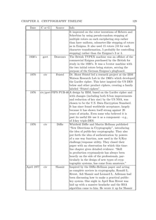
129. CHAPTER A. CRYPTOGRAPHY TIMELINE 123
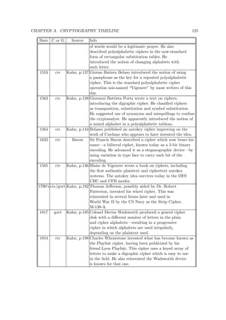
Date C or G Source Info
200’s civ Kahn, p.91 “The so-called Leiden papyrus [...] employes
cipher to conceal the crucial protions of
important magic recipes.”
725-790? govt/(civ) Kahn, p.97 Abu ‘Abd al-Rahman al-Khalil ibn Ahmad
ibn ‘Amr ibn Tammam al Farahidi al-Zadi
al Yahmadi wrote a (now lost) book on
cryptography, inspired by his solution
of a cryptogram in Greek for the
Byzantine emporer. His solution was
based on known (correctly guessed)
plaintext at the message start—a
standard cryptanalytic method, used
even in World War II agains Enigma
messages.
855 civ Kahn, p.93 Abu Bakr Ahmad ben ‘Ali ben Wahshiyya
an-Nabati published several cipher alphabets
which were traditionally used for magic.
— govt Kahn, p.94 “A few documents with ciphertext survive from
the Ghaznavid government of conquered Persia,
and one chronicler reports that high officials
were supplied with a personal cipher before
setting out for new posts. But the general
lack of continuity of Islamic states and the
consequent failure to develop a permanent
civil service and to set up permanent
embassies in other countries militated against
cryptography’s more widespread use.”
1226 govt Kahn, p.106 “As early as 1226, a faint political
cryptography appeared in the archives of
Venice, where dots or crosses replaced
the vowels in a few scattered words.”
about 1250 civ Kahn, p.90 Roger Bacon not only descibed several
ciphers but wrote: “A man is crazy who
writes a secret in any other way than
one which will conceal it from the vulgar.”
1379 govt/civ Kahn, p.107 Gabrieli di Lavinde at the request of Clement
VII, compiled a combination substitution
alphabet and small code—the first example
of the nomenclator Kahn has found. This class
of code/cipher was to remain in general use
among diplomats and some civilians for the
next 450 years, in spite of the fact that
there were stronger ciphers being invented
in the meantime, possibly because of its
relative convenience.

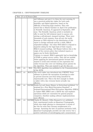
130. CHAPTER A. CRYPTOGRAPHY TIMELINE 124
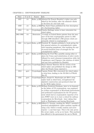
Date C or G Source Info
1300’s govt Kahn, p.94 ‘Abd al-Rahman Ibn Khaldun wrote “The
Muqaddimah”, a substantial survey of history which
cites the use of “names of perfums, fruits, birds,
or flowers to indicate the letters, or [...] of
forms different from the accepted forms of the
letters” as a cipher among tax and army bureaus. He
also includes a reference to cryptanalysis, noting
“Well-known writings on the subject are in the
possession of the people.”
1392 civ Price, p.182-7 “The Equatorie of the Planetis”, possibly written
by Geoffrey Chaucer, contains passages in cipher.
The cipher is a simple substitution with a cipher
alphabet consisting of letters, digits and symbols.
1412 civ Kahn, p.95-6 Shihab al-Din abu ‘l-‘Abbas Ahmad ben ‘Ali ben
Ahmand‘ Abd Allah al-Qalqashandi wrote “Subh al-a
‘sha”, a 14-volume Arabic encyclopedia which inclu-
ded a section on cryptology. This information was
attributed to Taj ad-Din ‘Ali ibn ad-Daraihim be
Muhammad ath-Tha‘alibi al-Mausili who lived from
1312 to 1361 but whose writings on cryptology have
been lost. The list of ciphers in this work included
both substitution and transposition and, for the first
time a cipher with multiple substitutions for each
plaintext letter. Also traced to Ibn al-Durauhim is
an exposition on and worked example of cryptanaly-
sis including the use of tables of letter frequencies
and sets of letters which cannot occur together in
one word.
1466-7 civ Kahn, p.127 Leon Battista Alberti invented and published the first
polyalphabetic cipher, designing a cipher disk (known
as the Captain Midnight Decoder Badge) to simplify
the process. This class of cipher was apparently not
broken until the 1800’s. Alberti also wrote extensively
on the state of the art in ciphers, besides his own
invention. Alberti also used his disk for enciphered
code. These systems were much stronger than the
nomenclator in use by the diplomats of the day and
for centuries to come.
1473-1490 civ Kahn, p.91 “A manuscript [...] by Arnaldus de Bruxella uses five
lines of cipher to conceal the crucial part of the
operation of making a philosopher’s stone.”
1518 civ Kahn, p.130-6 Johannes Trithemius wrote the first printed book on
cryptology. He invented a steganographic cipher in
which each letter was represented as a word taken
from a succession of columns. The resulting series

131. CHAPTER A. CRYPTOGRAPHY TIMELINE 125
Date C or G Source Info
of words would be a legitimate prayer. He also
described polyalphabetic ciphers in the now-standard
form of rectangular substitution tables. He
introduced the notion of changing alphabets with
each letter.
1553 civ Kahn, p.137 Giovan Batista Belaso introduced the notion of using
a passphrase as the key for a repeated polyalphabetic
cipher. This is the standard polyalphabetic cipher
operation mis-named “Vigenere” by most writers of this
day.
1563 civ Kahn, p.138 Giovanni Battista Porta wrote a text on ciphers,
introducing the digraphic cipher. He classified ciphers
as transposition, substitution and symbol substitution.
He suggested use of synonyms and misspellings to confuse
the cryptanalyst. He apparently introduced the notion of
a mixed alphabet in a polyalphabetic tableau.
1564 civ Kahn, p.144 Belasso published an autokey cipher improving on the
work of Cardano who appears to have invented the idea.
1623 civ Bacon Sir Francis Bacon described a cipher which now bears his
name—a biliteral cipher, known today as a 5-bit binary
encoding. He advanced it as a steganographic device—by
using variation in type face to carry each bit of the
encoding.
1585 civ Kahn, p.146 Blaise de Vigenere wrote a book on ciphers, including
the first authentic plaintext and ciphertext autokey
systems. The autokey idea survives today in the DES
CBC and CFB modes.
1790’s civ/govt Kahn, p.192 Thomas Jefferson, possibly aided by Dr. Robert
Patterson, invented his wheel cipher. This was
reinvented in several forms later and used in
World War II by the US Navy as the Strip Cipher,
M-138-A.
1817 govt Kahn, p.195 Colonel Decius Wadsworth produced a geared cipher
disk with a different number of letters in the plain
and cipher alphabets—resulting in a progressive
cipher in which alphabets are used irregularly,
depending on the plaintext used.
1854 civ Kahn, p.198 Charles Wheatstone invented what has become known as
the Playfair cipher, having been publicized by his
friend Lyon Playfair. This cipher uses a keyed array of
letters to make a digraphic cipher which is easy to use
in the field. He also reinvented the Wadsworth device
is known for that one.

132. CHAPTER A. CRYPTOGRAPHY TIMELINE 126
Date C or G Source Info
1857 civ Kahn, p.202 Admiral Sir Francis Beaufort’s cipher was pub-
lished by his brother, after the admiral’s death
in the form of a 4x5 inch card.
1859 civ Kahn, p.203 Pliny Earle Chase published the first description
of a fractionating cipher.
1854 civ Cryptologia Charles Babbage seems to have reinvented the
wheel cipher.
1861-1980 civ Deavourse “A study of United States patents from the issu-
ance of the first cryptographic patent in 1861
through 1980 identified 1,769 patents which are
primarily related to cryptography.”
1861 civ/(govt) Kahn, p.207 Friedrich W. Kasiski published a book giving the
first general solution of a polyalphabetic cipher
with repeating passphrase, thus marking the end
of several hundred years of strength for the
polyalphabetic cipher.
1861-5 govt Kahn, p.215 During the Civil War, possibly among other ci-
phers the Union used substitution of select words
followed by word columnar-transposition while the
Confederacy used Vigenere (the solution of which
had just been published by Kasiski).
1891 govt/(civ) Cryptologia Major Etienne Bazeries did his version of the
wheel cipher and published the design in 1901
after the French Army rejected it.
1913 govt Cryptologia Captain Parket Hitt reinvented the wheel cipher,
in strip form, leading to the M-138-A of World
War II.
1916 govt Cryptologia Major Joseph O. Mauborgne put Hitt’s strip
cipher back in wheel form, strengthened the
alphabet construction and produced what led
to the M-94 cipher device.
1917 civ Kahn, p.371 William Frederick Friedman, later to be honored
as the father of US cryptanalysis, was employed
as civilian cryptanalyst at Riverbank Laboratories
and performed cryptanalysis for the US govern-
ment which had no cryptanalytic expertise of its
own WWF went on to start a school for military
cryptanalysis for Riverbank—later taking that
work to Washington and leaving Riverbank.
1917 civ Kahn, p.401 Gilbert S. Vernam, working for AT&T, invented a
practical polyalphabetic cipher machine capable of
using a key which is totally random and never
repeats—a one-time-tape. This is the only prova-
bly secure cipher, as far as we know. This machine
was offered to the government for use in World

133. CHAPTER A. CRYPTOGRAPHY TIMELINE 127
Date C or G Source Info
War I but it was rejected. It was put on the
commercial market in 1920.
1918 govt Kahn, p.304-5 The ADFGVX system was put into service by the
Germans near the end of World War I. This was a
cipher which performed a substitution through a
keyed array, fractionation and then transpostion
of a letter fractions. It was broken by the French
cryptanalyst, Lieutenant Georges Painvin.
1919 civ Kahn, p.420 Hugo Alexander Koch filed a patent in the Nether-
lands on a rotor based cipher machine. He assigned
these patent rights in 1927 to Arthur Scherbius
who invented and had been marketing the Enigma
machine since about 1923.
1919 civ Kahn, p.422 Arvid Gerhard Damm applied for a patent in Sweden
for a mechanical rotor cipher machine. This machine
grew into a family of cipher machines under the
direction of Boris Caesar Wilhelm Hagelin who took
over the business and was the only one of the
commercial cryptographers of this period to make a
thriving business. After the war, a Swedish law
which enabled the government to appropriate inven-
tions it felt important to defense caused Hagelin
to move the company to Zug Switzerland where it was
incorporated as Crypto AG. The company is still in
operation although facing controversy for having
allegedly weakened a cipher product for sale to
Iran.
1921 civ Kahn, p.415 Edward Hugh Hebern incorporated “Hebern Electric
Code”, a company making electro-mechanical cipher
machines based on rotors which turn, odometer style,
with each character enciphered.
1923 civ Kahn, p.421 Arthur Scherbius incorporated “Chiffriermaschinen
Aktiongesellschaft” to make and sell his Enigma
machine.
1924 civ Deavours, p.151 Alexander von Kryha produced his “coding machine”
which was used, even by the German Diplomatic
Corps into the 1950s. However, it was cryptographi-
cally weak—having a small period. A test crypto-
gram of 1135 characters was solved by the US crypt-
analysts Friedman, Kullback, Rowlett and Sinkov in
2 hours and 41 minutes. Nevertheless, the machine
continued to be sold and used—a triumph of sales-
manship and a lesson to consumers of cryptographic
devices.

134. CHAPTER A. CRYPTOGRAPHY TIMELINE 128
Date C or G Source Info
1927-33 civ Kahn, p.802ff Users of cryptography weren’t limited to legitimate
bankers, lovers, experimenters, etc. There were also
a handful of criminals. “The greatest era of
international smuggling—Prohibition—created the
greatest era of criminal cryptology.” To this day,
the FBI runs a cryptanalytic office to deal with
criminal cryptography.
“A retired lieutenant commander of the Royal Navy
devised the systems for Consolidated Exporters’
Pacific operation, though its Gulf and Atlantic
groups made up theri own as needed.”
“His name was unknown but his cryptanalytic exper-
tise was apparent. The smugglers’ systems grew in-
creasingly more complicated. “Some of these are of
a complexity never even attempted by any government
for its most secret communications,” wrote Mrs.
Friedman in a report in mid-1930. “At no time
during the World War, when secret methods of
communication reached their highest development,
were there used such involved ramifications as are
to be found in some of the correspondence of West
Coast rum running vessels.””
1929 civ Kahn, p.404 Lester S. Hill published “Cryptography in an Algebraic
Alphabet” in which a block of plaintext is enciphered
by a matrix operation.
1933-45 govt Kahn, p.422 The Enigma machine was not a commercial success but
it was taken over and improved upon to become the
cryptographic workhouse of Nazi Germany. It was
broken by the Polish mathematician, Marian Rejewski,
based only on captured ciphertext and one list of
three month worth of daily keys obtained through a
spy. Continued breaks were based on developments
during the war by Alan Turing, Gordon Welchman and
others at Bletchley Park in England.
1937 govt Kahn, p.18ff The Japanese Purple machine was invented in response
to revelations by Herbert O. Yardley and broken by a
team headed by William Frederick Friedman. The
Purple machine used telephone stepping relays instead
of rotors and thus had a totally different permuta-
tion at each step rather than the related permuta-
tions of one rotor in different positions.
1930’s govt Kahn, p.510ff Kahn attributes the American SIGABA (M-134-C) to
William F. Friedman while Deavours attributes it to an
idea of Frank Rowlett, one of Friedman’s first hires.

135. CHAPTER A. CRYPTOGRAPHY TIMELINE 129
Date C or G Source Info
It improved on the rotor inventions of Hebern and
Scherbius by using pseudo-random stepping of
multiple rotors on each enciphering step rather
than have uniform, odometer-like stepping of rotors
as in Enigma. It also used 15 rotors (10 for each
character transformation, 5 probably for controlling
stepping) rather than the Enigma’s 3 or 4.
1930’s govt Deavours The British TYPEX machine was an offshot of the
commercial Enigma purchased by the British for
study in the 1920’s. It was a 5-rotor machine with
the two initial rotors being stators, serving the
purpose of the German Enigma’s plugboard.
1970 civ Feistel Dr. Horst Feistel led a research project at the IBM
Watson Research Lab in the 1960’s which developed
the Lucifer cipher. This later inspired the US DES
below and other product ciphers, creating a family
labeled “Feistel ciphers”.
1976 civ/govt FIPS PUB-46 A design by IBM, based on the Lucifer cipher and
with changes (including both S-box improvements
and reduction of key size) by the US NSA, was
chosen to be the U.S. Data Encryption Standard.
It has since found worldwide acceptance, largely
because it has shown itself strong against 20
years of attacks. Even some who believed it is
past its useful life use it as a component—e.g.,
of 3-key triple-DES.
1976 civ Diffie Whitfield Diffie and Martin Hellman published
“New Directions in Cryptography”, introducing
the idea of public-key cryptography. They also
put forth the idea of authentication by powers
of a one way function, now used in the S/Key
challenge/response utility. They closed their
paper with an observation for which this time-
line chapter gives detailed evidence: “Skill
in production cryptanalysis has always been
heavily on the side of the professionals, par-
ticularly in the design of new types of cryp-
tographic systems, has come from amateurs.”
April 1977 civ Shamir Inspired by the Diffie-Hellman paper and acting
as complete novices in cryptography, Ronald L.
Rivest, Adi Shamir and Leonard L. Adleman had
been discussing how to make a practical public-
key system. One night in April Ron Rivest was
laid up with a massive headache and the RSA
algorithm came to him. He wrote it up for Shamir

136. CHAPTER A. CRYPTOGRAPHY TIMELINE 130
Date C or G Source Info
and Adleman and sent it to them the next morning. It
was a practical public-key cipher for both confi-
dentiality and digital signatures, based on the
difficulty of factoring large numbers. They sub-
mitted this to Martin Gardner on April 4 for publication
in Scientific American. It appeared in September, 1977
issue. The Scientific American article is included an
offer to send the full technical report to anyone sub-
mitting a self-adressed, stamped envelope. There were
thousands of such requests, from all over the world.
Someone at NSA objected to the distribution of this
report to foreign nationals and for a while, RS&A
suspended mailings—but when NSA failed to respond to
inqueries asking for the legal basis of their request,
RS&A resumed mailings. Adi Shamir believes this is the
origin of the current policy that technical reports or
papers can be freely distributed.
Contrary to rumour, RS&A apparantly had no knowledge
of ITAR or patent secrecy orders. They did not publish
before applying for international patents because they
wanted to avoid such restrains on free expression but
rather because they were not thinking about patents for
the algorithm. They just wanted to get the idea out.
1978 civ RSA The RSA algorithm was published in the Communications
of the ACM.
1984-5? civ ROT13 The rot13 cipher was introduced into USENET News
software to permit the encryption of postings in order
to prevent innocent eyes from being assaulted by
objectionable text. This is the first example in which
a cipher with a key everyone knows actually was
effective.
1990 civ IACR90 Xuejia Lai and James Massey in Switzerland published “A
proposal for a New Block Encryption Standard”, a
proposed International Data Encryption Algorithm (IDEA)
to replace DES. IDEA uses a 128-bit key and employes
operations which are convenient for general purpose
computers, therefore making software implementations
more efficient.
1990 civ IACR90 Charles H. Bennett, Gilles Brassard et al. published
their experimental results on Quantum Cryptography,
which uses single photons to communicate a stream of
key bits for some later Vernam encipherment of a
message. Assuming the laws of quantum mechanics hold,
Quantum Cryptography provides not only secrecy but a
positive indication of eavesdropping and a measurement

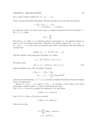
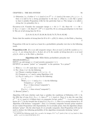
137. CHAPTER A. CRYPTOGRAPHY TIMELINE 131
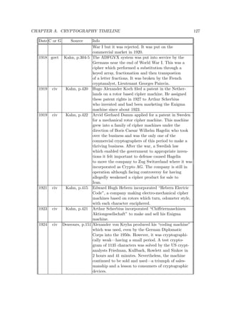
Date C or G Source Info
of the maximum number of bits an eavesdropper might
have captured. On the downside, QC currently requires
a fibre-optic cable between two parties.
1991 civ Garfinkel Phil Zimmerman released his first version of PGP
(Pretty Good Privacy) in response to the threat by
the FBI to demand access to the cleartext of the
communications of citizens. PGP offered high security
to the general citizen and as such could have been
seen as a competitor to commercial products like
Mailsafe from RSADSI. However, PGP os especially
notable because it was released as freeware and has
become a worldwide standard as a result while its
competitors of the time remain effictively unknown.
1994 civ Rivest Professor Ron Rivest, author of the earlier RC2 and
RC4 algorithms included in RSADSI’s BSAFE
cryptographic library, published a proposed algorithm,
RC5, on the Internet. This algorithm uses
data-dependent rotation as its non-linear operation
and is parameterized so that the user can vary the
block size, number of rounds and key length.
The cited sources are:
– Bacon: Sir Francis Bacon, “De Augmentis Scientarum”, Book 6, Chapter i. [as quoted in
C. Stopes, “Bacon-Shakspere Question”, 1889]
– Burton: Sir Richard F. Burton trans., “The Kama Sutra of Vatsayana”, Arkana/Penguin,
1991.
– Deavours: Cipher A. Deavours and Louis Kruh, “Machine Cryptography and Modern
Cryptanalysis”, Artech House, 1985.
– Diffie: Whitfield Diffie and Martin Hellman, “New Directions in Cryptography”, IEEE
Transactions on Information Theory, Nov 1976.
– Feistel: Horst Feistel, “Cryptographic Coding for Data-Bank Privacy”, IBM Research
Report RC2827.
– Garfinkel, Simson: “PGP: Pretty Good Privacy”, O’Reilly & Associates, Inc., 1995.
– IACR90: Proceedings, EUROCRYPT ’90; Springer Verlag.
– Kahn: David Kahn, “The Codebreakers”, Macmillan, 1967.
– Price: Derek J. Price, “The Equatorie of the Planetis”, edited from Peterhouse MS 75.I,
Cambridge University Press, 1955.
– Rivest: Ronald L. Rivest, “The RC5 Encryption Algorithm”, document made available
by FTP and World Wide Web, 1994.
– ROT13: S. Bellovin and M. Ranum, individual personal communications, July 1995.
– RSA: Rivest, Shamir and Adleman, “A method for obtaining digital signatures and public
key cryptosystems”, Communications of the ACM, Feb. 1978, pp. 120-126.
– Shamir: Adi Shamir, “Myths and Realities”, invited talk at CRYPTO ’95, Santa Barbara,
CA; August 1995.

138. Bibliography
[Stinson (1995)] D. R. Stinson. Cryptography and Practice. CRC Press. 1995.
The book is currently one of the most used introductory textbooks in the field of cryptog-
raphy. It contains various topics of this area which cannot all be treated within the paper.
Our paper will be based on the first chapters of this book that constitute a standard in-
troduction into that field. In fact, these topics are Classical Cryptosystems, The Data
Encryption Standard, The RSA System and The ElGamal Cryptosystem. Time permit-
ting we may also cover Frequencies (Chapter two). The book is highly recommended not
only as an accompanying book but also for further reading.
[Menezes, van Oorschot, Vanstone (1996)] A. Menezes, P. van Oorschot, S.Vanstone. Hand-
book of Applied Cryptography . CRC Press. 1996.
This book can be regarded as the standard reference book. It is full of important in-
formation for almost all topics on cryptography. We will use the book as a source for
algorithms which are fundamental in view of applications. It is recommended you have
a look at chapters 1,2,3, 7 and 8 to become acquainted with definitions and facts for
relevant topics of the paper and especially at all of chapter 1 to get an overview into
what directions cryptography might lead. Whenever you need a specific fact concerning
cryptography, this is the book you will find it in or at least a respective reference.
[Koblitz (1994)] N. Koblitz. A Course in Number Theory and Cryptography. Springer-Verlag.
1994.
This book attaches particular importance to the mathematical background of cryptog-
raphy. It handles certain topics that are based on results of number theory and gives,
therefore, an introduction to this branch, especially to modular arithmetic, prime num-
bers and finite fields. The paper is intended to dispense with proofs of the book but not
to dispense with the facts given. It is recommended you have a read through chapters 1
to 4. The more you understand, the easier you will find the paper.
[Koblitz (1999)] N. Koblitz: Algebraic Aspects of Cryptography. Springer-Verlag. 1999.
As the name already reveals, this book emphasizes on algebraic methods used in cryptog-
raphy. It starts off with a self-contained introduction to basic concepts and techniques.
This includes ideas from complexity theory and in particular algebra. The next chapters
and the appendix contain material that for the most part has not previously appeared in

139. BIBLIOGRAPHY 133
textbook form. A novel feature is the inclusion of three types of cryptography - ”hidden
monomial” systems, combinatorial-algebraic systems, and hyperelliptic systems - that
are at an early stage of development.
[Ivan Damgard (Ed.)] I. Damgard: Lectures on Data Security - Modern Cryptology in Theory
and Practice. Springer-Verlag. Lecture Notes in Computer Science 1561. 1999.
In July 1998, a summer school in cryptology and data security was organized at the
computer science department of Aarhus University, Denmark. A total of 13 speakers
gave a talk on main areas, covering both theoretical and practical topics. The book con-
tains all these papers, that serve an educational purpose: elementary introductions are
given to a number of subjects, some examples are given of the problems encountered,
as weel as solutions, open problems, and references for further reading. The papers are:
”Practice-Oriented Provable Security”, ”Introduction to Secure Computation”, ”Com-
mitment Schemes and Zero-Knowledge Protocols”, ”Emerging Standards for Public-Key
Cryptography”, ”Contemporary Block-Ciphers”, ”Primality Tests and Use of Primes
in Public-Key Systems”, ”Signing Contracts and Paying Electronically”, ”The State of
Cryptographic Hash Functions”, ”The Search for the Holy Grail in Quantum Cryptog-
raphy” and ”Unconditional Security in Cryptography”.
[Paul Garrett] Paul Garrett: Making, Breaking Codes - An Introduction to Cryptology. Pren-
tice Hall. 2001.
This is another very good introduction into the field. Apart from the description of some
block ciphers, this book covers every topic of our course and more. As an introductory
work, the reader can find heaps of examples and exercises in it.
[C. H. Papadimitriou] Christos H. Papadimitriou: Computational Complexity. Addison-
Wesley. 1995
This book is included in the list because of the close relationship of cryptography and
complexity theory. It is an excellent introduction into fundamental ideas of complexity
that are indispensable for a deeper understanding of modern cryptography. The book goes
far beyond the purposes of our course, but is highly recommended for further reading on
one of the most interesting and challenging topic in our time.
[W. Stallings] William Stallings: Cryptography and Network Security: Principles and Prac-
tices. Prentice Hall. 2003
Stalling has provided a staste-of-the-art text covering the basic issues and principles and
surveying cryptographic and network security techniques. The latter part of the book
deals with the real-world practice of network security: practical applications that have
been implemented and are in use to provide network security. This book is intended for
both an academic and a professional audience. Make sure you buy the third edition, if
you buy.

140. BIBLIOGRAPHY 134
[Pieprzyk, Hardjono, Seberry] Josef Pieprzyk, Thomas Hardjono, Jennifer Seberry: Funda-
mentals of Computer Security. Springer. 2003
This book presents modern concepts of computer security. It introduces the basic math-
ematical background necessary to follow computer security concepts. Modern develop-
ments in cryptography are examined, starting from private-key and public-key encryp-
tion, going through hashing, digital signitures, authentication, secret sharing, group-
oriented cryptorgraphy, pseudorandomness, key establishment protocols, zero-knowledge
protocols, and identification, and finishing with an introduction to modern e-business
systems based on digital cash. Intrusion detection and access control provide examples
of security systems implemented as a part of operating system. Database and network
security are also discussed. This book has just been released.