ippr note

1. Image Processing and Pattern
Recognition (IPPR):
(Lecture 2)
Sanjeeb Prasad Panday
sanjeeb77@hotmail.com

2. 2
of
92
Digital image representation
Monochrome image (or simply image) refers to a
2- dimensional light intensity function f(x,y)
– x and y denote spatial coordinates
– the value of f(x,y) at (x,y) is proportional to the brightness
(or gray level) of the image at that point

3. 3
of
92
Digital image representation
A digital image is an image f(x,y) that has been
discretized both in spatial coordinates and in
brightness
• Considered as a matrix whose row and column
indices represent a point in the image
• The corresponding matrix element value
represents the gray level at that point
• The elements of such an array are referred to as:
– image elements
– picture elements (pixels or pels)

4. 4
of
92
Steps in image processing
The problem domain in this example consists of pieces of mail
and the objective is to read the address on each piece
Step 1: image acquisition
– Acquire a digital image using an image sensor
• a monochrome or color TV camera: produces an entire image of the
problem domain every 1/30 second
• a line-scan camera: produces a single image line at a time, motion past the
camera produces a 2-dimensional image
– If not digital, an analog-to-digital conversion process is required
– The nature of the image sensor (and the produced image) are
determined by the application
• Mail reading applications rely greatly on line-scan cameras
• CCD and CMOS imaging sensors are very common in many applications

5. 5
of
92
Steps in image processing
• Step 2: preprocessing
– Key function: improve the image in ways that increase the
chance for success of the other processes
– In the mail example, may deal with contrast enhancement,
removing noise, and isolating regions whose texture indicates a
likelihood of alphanumeric information

6. 6
of
92
Steps in image processing
• Step 3: segmentation
– Broadly defined: breaking an image into its constituent parts
– In general, one of the most difficult tasks in image processing
• Good segmentation simplifies the rest of the problem
• Poor segmentation make the task impossible
– Output is usually raw pixel data: may represent region boundaries,
points in the region itself, etc.
• Boundary representation can be useful when the focus is on
external shape characteristics (e.g. corners, rounded edges, etc.)
• Region representation is appropriate when the focus is on
internal properties (e.g. texture or skeletal shape)
– For the mail problem (character recognition) both representations
can be necessary

7. 7
of
92
Steps in image processing
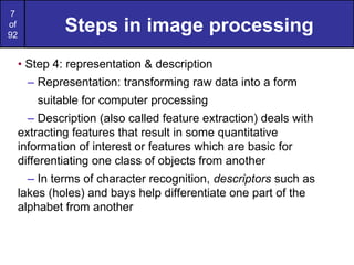
• Step 4: representation & description
– Representation: transforming raw data into a form
suitable for computer processing
– Description (also called feature extraction) deals with
extracting features that result in some quantitative
information of interest or features which are basic for
differentiating one class of objects from another
– In terms of character recognition, descriptors such as
lakes (holes) and bays help differentiate one part of the
alphabet from another

8. 8
of
92
Steps in image processing
• Step 5: recognition & interpretation
– Recognition: The process which assigns a label to an object
based on the information provided by its descriptors
A may be the alphanumeric character A
– Interpretation: Assigning meaning to an ensemble of
recognized objects
35487-0286 may be a ZIP code

9. 9
of
92
Steps in image processing

10. 10
of
92
Steps in image processing

11. 11
of
92
A Knowledge Base
• Knowledge about a problem domain is coded into an
image processing system in the form of a knowledge
database
– May be simple:
• detailing areas of an image expected to be of interest
– May be complex
• A list of all possible defects of a material in a vision inspection
system
– Guides operation of each processing module
– Controls interaction between modules
– Provides feedback through the system

12. 12
of
92
Steps in an image processing
system
• Not all image processing systems would require all
steps/processing modules
– Image enhancement for human visual perception may not go
beyond the preprocessing stage
• A knowledge database may not be required
• Processing systems which include recognition and
interpretation are associated with image analysis systems
in which the objective is autonomous (or at least partially
automatic)

13. 13
of
92
A simple imaging model
• An image is a 2-D light intensity function f(x,y)
• As light is a form of energy
0 < f(x,y) < ∞
• f(x,y) may be expressed as the product of 2 components
f(x,y)=i(x,y)r(x,y)
• i(x,y) is the illumination: 0 < i(x,y) < ∞
– Typical values: 9000 foot-candles sunny day, 100 office room, 0.01
moonlight
• r(x,y) is the reflectance: 0 < r(x,y) < 1
– r(x,y)=0 implies total absorption
– r(x,y)=1 implies total reflectance
– Typical values: 0.01 black velvet, 0.80 flat white paint, 0.93 snow

14. 14
of
92
A simple imaging model
• The intensity of a monochrome image f at (x,y) is the
gray level (l) of the image at that point
• In practice Lmin=imin rmin and Lmax=imax rmax
• As a guideline Lmin ≈ 0.005 and Lmax ≈ 100 for indoor
image processing applications
• The interval [Lmin, Lmax] is called the gray scale
• Common practice is to shift the interval to [0,L] where l=0
is considered black and l=L is considered white. All
intermediate values are shades of gray

15. 15
of
92
Sampling and Quantization
• To be suitable for computer processing an image, f(x,y) must
be digitized both spatially and in amplitude
• Digitizing the spatial coordinates is called image sampling
• Amplitude digitization is called gray-level quantization
• f(x,y) is approximated by equally spaced samples in the form
of an NxM array where each element is a discrete quantity

16. 16
of
92
Sampling and Quantization
• Common practice is to let N and M be powers of two;
N=2^n and M=2^k
• And G=2^m where G denotes the number of gray levels
• The assumption here is that gray levels are equally space in
the interval [0,L]
• The number of bits, b, necessary to store the image is then
• For example, a 128x128 image with 64 gray levels would
require 98,304 bits of storage

17. 17
of
92
Sampling and Quantization
• How many samples and gray levels are required for a “good”
approximation?
• The resolution (the degree of discernible detail) depends strongly on
these two parameters

18. 18
of
92
Effects of reducing spatial
resolution

19. 19
of
92
Effects of reducing gray levels

20. 20
of
92
Basic relationships between
pixels
 An image is denoted by: f(x,y)
 Lowercase letters (e.g. p, q) will denote individual pixels
 A subset of f(x,y) is denoted by S
 Neighbors of a pixel:
– A pixel p at (x,y) has 4 horizontal/vertical neighbors at
• (x+1,y),(x-1,y),(x,y+1)and(x,y-1)
• called the 4-neighbors of p: N4(p)
– A pixel p at (x,y) has 4 diagonal neighbors at
• (x+1,y+1),(x+1,y-1),(x-1,y+1)and(x-1,y-1)
• called the diagonal–neighbors of p:ND(p)
– The 4-neighbors and the diagonal-neighbors of p are called
the 8-neighbors of p: N8(p)

21. 21
of
92
Connectivity between pixels
• Connectivity is an important concept in establishing boundaries
of object and components of regions in an image
• When are two pixels connected?
– If they are adjacent in some sense (say they are 4-neighbors)
– and, if their gray levels satisfy a specified criterion of similarity
(say they are equal)
• Example: given a binary image (e.g. gray scale = [0,1]), two pixels
may be 4-neighbors but are not considered connected unless they
have the same value

22. 22
of
92
Connectivity between pixels
• Let V be the set of values used to determine connectivity
– For example, in a binary image, V={1} for the connectivity of pixels
with a value of 1
– In a gray scale image, for the connectivity of pixels with a range of
intensity values of, say, 32 to 64, it follows that V={32,33,...,63,64}
– Consider three types of connectivity
• 4-connectivity: Pixels p and q with values from V are 4-connected if q is
in the set N4(p)
• 8-connectivity: Pixels p and q with values from V are 8-connected if q is
in the set N8(p)
• m-connectivity (mixed): Pixels p and q with values from V are
m-connected if
– q is in the set N4(p),or
– q is in the set ND(p) and the set N4(p) ∩ N4(q) is empty (This is the set of
pixels that are 4-neighbors of p and q and whose values are from V)

23. 23
of
92
Connectivity between pixels

24. 24
of
92
Pixel adjacencies and paths
• Pixel p is adjacent to q if they are connected
– We can define 4-, 8-, or m-adjacency depending on the
specified type of connectivity
• Two image subsets S1 and S2 are adjacent if some pixel in S1
is adjacent to S2
• A path from p at (x,y) to q at (s,t) is a sequence of distinct
pixels with coordinates (x0,y0), (x1,y1),....., (xn,yn)
– Where (x0,y0)=(x,y) and (xn,yn)=(s,t) and
– (xi,yi) is adjacent to (xi-1,yi-1) for 1<= i <= n
– n is the length of the path
• If p and q are in S, then p is connected to q in S if there is a
path from p to q consisting entirely of pixels in S

25. 25
of
92
Example paths

26. 26
of
92
Connected components
• For any pixel p in S, the set of pixels connected to p form a
connected component of S
• Distinct connected components in S are said to be disjoint

27. 27
of
92
Labeling 4-connected
components
• Consider scanning an image pixel by pixel from left to right and
top to bottom
– Assume, for the moment, we are interested in 4-connected
components
– Let p denote the pixel of interest, and r and t denote the
upper and left neighbors of p, respectively
– The nature of the scanning process assures that r and t have
been encountered (and labeled if 1) by the time p is
encountered

28. 28
of
92
Labeling 4-connected
components
• Consider the following procedure
if p=0 continue to the next position
if r=t=0 assign a new label to p (Ln)
if r=t=1 and they have the same label, assign that label to p
if only one of r and t are 1, assign its label to p
if r=t=1 and they have different labels, assign one label to p and
note that the two labels are equivalent (that is r and t are connected
through p)
At the end of the scan, sort pairs of equivalent labels into
equivalence classes and assign a different label to each class

29. 29
of
92
Labeling 4-connected
components (example)

30. 30
of
92
Labeling 8-connected
components
• Proceed as in the 4-connected component labeling case, but
also examine two upper diagonal neighbors (q and s) of p

31. 31
of
92
Labeling connected components
in non-binary images
• The 4-connected or 8-connected labeling schemes can be
extended to gray level images
• The set V may be used to connect into a component only
those pixels within a specified range of pixel values

32. 32
of
92
Distance measures
• Given pixels p, q, and z at (x,y), (s,t) and (u,v) respectively,
• D is a distance function (or metric) if:
– D(p,q) ≥ 0 (D(p,q)=0 iff p=q),
– D(p,q) = D(q,p), and
– D(p,z) ≤ D(p,q) + D(q,z).
• The Euclidean distance between p and q is given by:
• The pixels having distance less than or equal to some value r
from (x,y) are the points contained in a disk of radius r centered
at (x,y)

33. 33
of
92
Distance measures
• The D4 distance (also called the city block distance) between p
and q is given by:
• The pixels having a D4 distance less than some r from (x,y)
form a diamond centered at (x,y)
• Example: pixels where D4 ≤ 2

34. 34
of
92
Distance measures
• The D8 distance (also called the chessboard distance)
between p and q is given by:
• The pixels having a D8 distance less than some r from (x,y)
form a square centered at (x,y)
• Example: pixels where D8 ≤ 2

35. 35
of
92
Distance measures and
connectivity
• The D4 distance between two points p and q is the shortest 4-
path between the two points
• The D8 distance between two points p and q is the shortest 8-
path between the two points
• D4 and D8 may be considered, regardless of whether a
connected path exists between them, because the definition of
these distances involves only the pixel coordinates
• For m-connectivity, the value of the distance (the length of the
path) between two points depends on the values of the pixels
along the path

36. 36
of
92
Distance measures and m-
connectivity
• Consider the given arrangement of pixels and assume
– p, p2 and p4 =1
– p1 and p3 can be 0 or 1
• If V={1} and p1 and p3 are 0, the m-distance (p, p4) is 2 If either
p1 or p3 are 1, the m-distance (p, p4) is 3 If p1 and p3 are 1, the
m-distance (p, p4) is 4

37. 37
of
92
M-connectivity example

38. 38
of
92
Arithmetic & logic operations
• Arithmetic & logic operations on images used extensively in
most image processing applications
– May cover the entire image or a subset Arithmetic operation
between pixels p and q are defined as:
– Addition: (p+q)
• Used often for image averaging to reduce noise
– Subtraction: (p-q)
• Used often for static background removal
– Multiplication: (p*q) (or pq, p×q)
• Used to correct gray-level shading
– Division: (p÷q) (or p/q)
• As in multiplication

39. 39
of
92
Logic operations
• Arithmetic operation between pixels p and q are defined as:
– AND: p AND q (also p⋅q)
– OR: p OR q (also p+q)
– COMPLEMENT: NOTq (also q’)
• Form a functionally complete set
• Applicable to binary images
• Basic tools in binary image processing, used for:
– Masking
– Feature detection
– Shape analysis

40. 40
of
92
Examples of logic operations

41. 41
of
92
Examples of logic operations

42. 42
of
92
Neighborhood-oriented
operations
• Arithmetic and logical operations may take place on a
subset of the image
– Typically neighborhood oriented
• Formulated in the context of mask operations (also
called template, window or filter operations)
• Basic concept:let the value of a pixel be a function of its
(current) gray level and the gray level of its neighbors (in
some sense)

43. 43
of
92
Neighborhood-oriented
operations
• Consider the following subset of pixels in an image
• Suppose we want to filter the image by replacing the value at
Z5 with the average value of the pixels in a 3x3 region centered
around Z5
• Perform an operation of the form:
• and assign to z5 the value of z

44. 44
of
92
Neighborhood-oriented
operations
• In the more general form, the operation may look like:
• This equation is widely used in image processing
• Proper selection of coefficients (weights) allows for operations
such as
– noise reduction
– region thinning
– edge detection

45. 45
of
92
What Is Image Enhancement?
Image enhancement is the process of
making images more useful
The reasons for doing this include:
– Highlighting interesting detail in images
– Removing noise from images
– Making images more visually appealing

46. 46
of
92
Image Enhancement Examples
Images
taken
from
Gonzalez
&
Woods,
Digital
Image
Processing
(2002)

47. 47
of
92
Image Enhancement Examples (cont…)
Images
taken
from
Gonzalez
&
Woods,
Digital
Image
Processing
(2002)

48. 48
of
92
Image Enhancement Examples (cont…)
Images
taken
from
Gonzalez
&
Woods,
Digital
Image
Processing
(2002)

49. 49
of
92
Image Enhancement Examples (cont…)
Images
taken
from
Gonzalez
&
Woods,
Digital
Image
Processing
(2002)

50. 50
of
92
Spatial & Frequency Domains
There are two broad categories of image
enhancement techniques
– Spatial domain techniques
• Direct manipulation of image pixels
– Frequency domain techniques
• Manipulation of Fourier transform or wavelet
transform of an image
For the moment we will concentrate on
techniques that operate in the spatial
domain

51. 51
of
92
Basic Spatial Domain Image
Enhancement
Origin x
y Image f (x, y)
(x, y)
Most spatial domain enhancement operations
can be reduced to the form
g (x, y) = T[ f (x, y)]
where f (x, y) is the
input image, g (x, y) is
the processed image
and T is some
operator defined over
some neighbourhood
of (x, y)

52. 52
of
92
Point Processing
The simplest spatial domain operations
occur when the neighbourhood is simply the
pixel itself
In this case T is referred to as a grey level
transformation function or a point processing
operation
Point processing operations take the form
s = T ( r )
where s refers to the processed image pixel
value and r refers to the original image pixel
value

53. 53
of
92
Point Processing Example:
Negative Images
Negative images are useful for enhancing
white or grey detail embedded in dark
regions of an image
– Note how much clearer the tissue is in the
negative image of the mammogram below
s = 1.0 - r
Original
Image
Negative
Image
Images
taken
from
Gonzalez
&
Woods,
Digital
Image
Processing
(2002)

54. 54
of
92
Point Processing Example:
Negative Images (cont…)
Original Image x
y Image f (x, y)
Enhanced Image x
y Image f (x, y)
s = intensitymax - r

55. 55
of
92
Point Processing Example:
Thresholding
Thresholding transformations are particularly
useful for segmentation in which we want to
isolate an object of interest from a
background
s =
1.0
0.0 r <= threshold
r > threshold
Images
taken
from
Gonzalez
&
Woods,
Digital
Image
Processing
(2002)

56. 56
of
92
Point Processing Example:
Thresholding (cont…)
Original Image x
y Image f (x, y)
Enhanced Image x
y Image f (x, y)
s =
0.0 r <= threshold
1.0 r > threshold

57. 57
of
92
Intensity Transformations
Images
taken
from
Gonzalez
&
Woods,
Digital
Image
Processing
(2002)

58. 58
of
92
Basic Grey Level Transformations
There are many different kinds of grey level
transformations
Three of the most
common are shown
here
– Linear
• Negative/Identity
– Logarithmic
• Log/Inverse log
– Power law
• nth
power/nth
root
Images
taken
from
Gonzalez
&
Woods,
Digital
Image
Processing
(2002)

59. 59
of
92
Logarithmic Transformations
The general form of the log transformation is
s = c * log(1 + r)
The log transformation maps a narrow range
of low input grey level values into a wider
range of output values
The inverse log transformation performs the
opposite transformation
Compresses the dynamic range of images
with large variations in pixel values

60. 60
of
92
Logarithmic Transformations (cont…)
Log functions are particularly useful when
the input grey level values may have an
extremely large range of values
In the following example the Fourier
transform of an image is put through a log
transform to reveal more detail
s = log(1 + r)
Images
taken
from
Gonzalez
&
Woods,
Digital
Image
Processing
(2002)

61. 61
of
92
Logarithmic Transformations (cont…)
Original Image x
y Image f (x, y)
Enhanced Image x
y Image f (x, y)
s = log(1 + r)
We usually set c to 1
Grey levels must be in the range [0.0, 1.0]

62. 62
of
92
Power Law Transformations
Power law transformations have the following
form
s = c * r γ
Map a narrow range
of dark input values
into a wider range of
output values or vice
versa
Varying γ gives a whole
family of curves
Images
taken
from
Gonzalez
&
Woods,
Digital
Image
Processing
(2002)

63. 63
of
92
Power Law Transformations (cont…)
We usually set c to 1
Grey levels must be in the range [0.0, 1.0]
Original Image x
y Image f (x, y)
Enhanced Image x
y Image f (x, y)
s = r γ

64. 64
of
92
Power Law Example

65. 65
of
92
Power Law Example (cont…)
γ = 0.6
0
0.1
0.2
0.3
0.4
0.5
0.6
0.7
0.8
0.9
1
0 0.2 0.4 0.6 0.8 1
Old Intensities
Transformed
Intensities

66. 66
of
92
Power Law Example (cont…)
γ = 0.4
0
0.1
0.2
0.3
0.4
0.5
0.6
0.7
0.8
0.9
1
0 0.2 0.4 0.6 0.8 1
Original Intensities
Transformed
Intensities

67. 67
of
92
Power Law Example (cont…)
0
0.1
0.2
0.3
0.4
0.5
0.6
0.7
0.8
0.9
1
0 0.2 0.4 0.6 0.8 1
Original Intensities
Transformed
Intensities
γ = 0.3

68. 68
of
92
Power Law Example (cont…)
The images to the
right show a
magnetic resonance
(MR) image of a
fractured human
spine
Different curves
highlight different
detail
s = r 0.6
s
=
r
0.4
s =
r 0.3
Images
taken
from
Gonzalez
&
Woods,
Digital
Image
Processing
(2002)

69. 69
of
92
Power Law Example

70. 70
of
92
Power Law Example (cont…)
γ = 5.0
0
0.1
0.2
0.3
0.4
0.5
0.6
0.7
0.8
0.9
1
0 0.2 0.4 0.6 0.8 1
Original Intensities
Transformed
Intensities

71. 71
of
92
Power Law Transformations (cont…)
An aerial photo
of a runway is
shown
This time
power law
transforms are
used to darken
the image
Different curves
highlight
different detail
Images
taken
from
Gonzalez
&
Woods,
Digital
Image
Processing
(2002)
s = r 3.0
s
=
r
4.0
s =
r 5.0

72. 72
of
92
Gamma Correction
Many devices used for image capture, display and printing
respond according to a power law
• The exponent in the power-law equation is referred to as
gamma
• The process of correcting for the power-law response is
referred to as gamma correction
• Example: – CRT devices have an intensity-to-voltage
response that is
a power function (exponents typically range from 1.8-2.5)
– Gamma correction in this case could be achieved by
applying the transformation s=r1/2.5=r^0.4

73. 73
of
92
Gamma Correction
Many of you might be familiar with gamma
correction of computer monitors
Problem is that
display devices do
not respond linearly
to different
intensities
Can be corrected
using a log
transform
Images
taken
from
Gonzalez
&
Woods,
Digital
Image
Processing
(2002)

74. 74
of
92
More Contrast Issues
Images
taken
from
Gonzalez
&
Woods,
Digital
Image
Processing
(2002)

75. 75
of
92
Piecewise Linear Transformation
Functions
Rather than using a well defined mathematical
function we can use arbitrary user-defined
transforms
The images below show a contrast stretching
linear transform to add contrast to a poor
quality image
Images
taken
from
Gonzalez
&
Woods,
Digital
Image
Processing
(2002)

76. 76
of
92
Piecewise Linear Transformation
Functions
• Rather than using a well defined mathematical function we can use
arbitrary user-defined transforms
• Contrast stretching expands the range of intensity levels in an image so it
spans a given (full) intensity range
• Control points (r1,s1) and (r2,s2) control the shape of the transform T(r)
• r1=r2, s1=0 and s2=L-1 yields a thresholding function
The contrast stretched image shown in the previous slide is obtained using
the transformation obtained from the equation of the line having following
points
• (r1,s1)=(rmin,0) and (r2, s2)=(rmax,L-1)
Images
taken
from
Gonzalez
&
Woods,
Digital
Image
Processing
(2002)

77. 77
of
92
Gray Level Slicing
• Used to highlight a specific range of intensities in an
image that might be of interest
•Two common approaches
– Set all pixel values within a range of interest to one
value (white) and all others to another value (black)
Produces a binary image
– Brighten (or darken) pixel values in a range of interest
and leave all others unchanged
Images
taken
from
Gonzalez
&
Woods,
Digital
Image
Processing
(2002)

78. 78
of
92
Gray Level Slicing
Highlights a specific range of grey levels
– Similar to thresholding
– Other levels can be
suppressed or maintained
– Useful for highlighting features
in an image
Images
taken
from
Gonzalez
&
Woods,
Digital
Image
Processing
(2002)

79. 79
of
92
Bit Plane Slicing
Often by isolating particular bits of the pixel
values in an image we can highlight
interesting aspects of that image
– Higher-order bits usually contain most of the
significant visual information
– Lower-order bits contain
subtle details
Images
taken
from
Gonzalez
&
Woods,
Digital
Image
Processing
(2002)

80. 80
of
92
Bit Plane Slicing (cont…)
Images
taken
from
Gonzalez
&
Woods,
Digital
Image
Processing
(2002)
[10000000] [01000000]
[00100000] [00001000]
[00000100] [00000001]

81. 81
of
92
Bit Plane Slicing (cont…)
Images
taken
from
Gonzalez
&
Woods,
Digital
Image
Processing
(2002)
[10000000] [01000000]
[00100000] [00001000]
[00000100] [00000001]

82. 82
of
92
Bit Plane Slicing (cont…)

83. 83
of
92
Bit Plane Slicing (cont…)
Images
taken
from
Gonzalez
&
Woods,
Digital
Image
Processing
(2002)

84. 84
of
92
Bit Plane Slicing (cont…)
Images
taken
from
Gonzalez
&
Woods,
Digital
Image
Processing
(2002)

85. 85
of
92
Bit Plane Slicing (cont…)
Images
taken
from
Gonzalez
&
Woods,
Digital
Image
Processing
(2002)

86. 86
of
92
Bit Plane Slicing (cont…)
Images
taken
from
Gonzalez
&
Woods,
Digital
Image
Processing
(2002)

87. 87
of
92
Bit Plane Slicing (cont…)
Images
taken
from
Gonzalez
&
Woods,
Digital
Image
Processing
(2002)

88. 88
of
92
Bit Plane Slicing (cont…)
Images
taken
from
Gonzalez
&
Woods,
Digital
Image
Processing
(2002)

89. 89
of
92
Bit Plane Slicing (cont…)
Images
taken
from
Gonzalez
&
Woods,
Digital
Image
Processing
(2002)

90. 90
of
92
Bit Plane Slicing (cont…)
Images
taken
from
Gonzalez
&
Woods,
Digital
Image
Processing
(2002)

91. 91
of
92
Bit Plane Slicing (cont…)
Images
taken
from
Gonzalez
&
Woods,
Digital
Image
Processing
(2002)

92. 92
of
92
Bit Plane Slicing (cont…)
Reconstructed image
using only bit planes 8
and 7
Reconstructed image
using only bit planes 8, 7
and 6
Reconstructed image
using only bit planes 7, 6
and 5
Images
taken
from
Gonzalez
&
Woods,
Digital
Image
Processing
(2002)