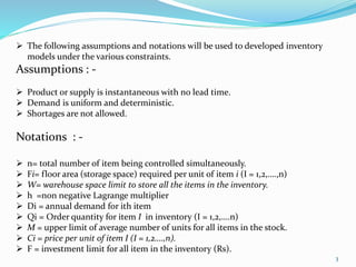
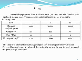
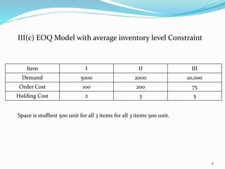
1
Presented By:-
Mitesh Chaudhari
Mihir Disawala
MULTI-ITEM INVENTORY MODEL - III
2
 An arrangement of controlling inventory of each item is only possible if there are
no constraints (limitations) on the total average inventory.
 This include : the total warehouse space, the total investment in inventories, or
the total number of order to be placed per year for all items; number of deliveries
which can be accepted; size of deliveries that can be handled, etc.
 Thus some modification of the optional order quantity determined in earlier
models has to be made in order to take care of such constraints.
 In this section, we will calculate EOQ for each item separately that minimize the
total inventory cost under the given constraints of limited warehouse capacity
and finance.
3
 The following assumptions and notations will be used to developed inventory
models under the various constraints.
Assumptions : -
 Product or supply is instantaneous with no lead time.
 Demand is uniform and deterministic.
 Shortages are not allowed.
Notations : -
 n= total number of item being controlled simultaneously.
 Fi= floor area (storage space) required per unit of item i (I = 1,2,….,n)
 W= warehouse space limit to store all the items in the inventory.
 h =non negative Lagrange multiplier
 Di = annual demand for ith item
 Qi = Order quantity for item I in inventory (I = 1,2,….n)
 M = upper limit of average number of units for all items in the stock.
 Ci = price per unit of item I (I = 1,2….,n).
 F = investment limit for all item in the inventory (Rs).
4
A small shop produces three machines parts I, II, III in lots. The shop has only
650 Sq. ft. storage space. The appropriate data for three items are given in the
following table.
Item I II III
Demand
rate(unit/year)
5,000 2,000 10,000
Order Cost 100 200 75
Cost / Unit 10 15 5
Floor space (Sq ft) 0.70 0.80 0.40
Sum
The shop uses an inventory carrying charge of 20% of average inventory valuation
Per year. If no stock outs are allowed, determine the optimal lot size for each item under
the given storage constraint.
5
III(b) EOQ Model with investment Constraint
A shop sells 3 item detail as given below find optional stock level for each item.
Average value of inventory shall not exceed 1000 Rs.
Item I II III
Carrying Cost 20 20 20
Order Cost 50 40 60
Cost / Unit 6 7 5
Annual Demand 10,000 12,000 7,500
6
III(c) EOQ Model with average inventory level Constraint
Item I II III
Demand 5000 2000 10,000
Order Cost 100 200 75
Holding Cost 2 3 5
Space is stuffiest 500 unit for all 3 items for all 3 items 500 unit.
7
8
III(d) EOQ Model with number of orders Constraint
Item I II
A 60.000 3
B 40,000 2
C 1,200 24
D 5,000 4
A company purchase four items with detail as below.
Company wants to restrict total orders to 40. Find numbers of order s for each item
9

Inventory Model 3 Operation Research

  • 1.
    1 Presented By:- Mitesh Chaudhari MihirDisawala MULTI-ITEM INVENTORY MODEL - III
  • 2.
    2  An arrangementof controlling inventory of each item is only possible if there are no constraints (limitations) on the total average inventory.  This include : the total warehouse space, the total investment in inventories, or the total number of order to be placed per year for all items; number of deliveries which can be accepted; size of deliveries that can be handled, etc.  Thus some modification of the optional order quantity determined in earlier models has to be made in order to take care of such constraints.  In this section, we will calculate EOQ for each item separately that minimize the total inventory cost under the given constraints of limited warehouse capacity and finance.
  • 3.
    3  The followingassumptions and notations will be used to developed inventory models under the various constraints. Assumptions : -  Product or supply is instantaneous with no lead time.  Demand is uniform and deterministic.  Shortages are not allowed. Notations : -  n= total number of item being controlled simultaneously.  Fi= floor area (storage space) required per unit of item i (I = 1,2,….,n)  W= warehouse space limit to store all the items in the inventory.  h =non negative Lagrange multiplier  Di = annual demand for ith item  Qi = Order quantity for item I in inventory (I = 1,2,….n)  M = upper limit of average number of units for all items in the stock.  Ci = price per unit of item I (I = 1,2….,n).  F = investment limit for all item in the inventory (Rs).
  • 4.
    4 A small shopproduces three machines parts I, II, III in lots. The shop has only 650 Sq. ft. storage space. The appropriate data for three items are given in the following table. Item I II III Demand rate(unit/year) 5,000 2,000 10,000 Order Cost 100 200 75 Cost / Unit 10 15 5 Floor space (Sq ft) 0.70 0.80 0.40 Sum The shop uses an inventory carrying charge of 20% of average inventory valuation Per year. If no stock outs are allowed, determine the optimal lot size for each item under the given storage constraint.
  • 5.
    5 III(b) EOQ Modelwith investment Constraint A shop sells 3 item detail as given below find optional stock level for each item. Average value of inventory shall not exceed 1000 Rs. Item I II III Carrying Cost 20 20 20 Order Cost 50 40 60 Cost / Unit 6 7 5 Annual Demand 10,000 12,000 7,500
  • 6.
    6 III(c) EOQ Modelwith average inventory level Constraint Item I II III Demand 5000 2000 10,000 Order Cost 100 200 75 Holding Cost 2 3 5 Space is stuffiest 500 unit for all 3 items for all 3 items 500 unit.
  • 7.
  • 8.
    8 III(d) EOQ Modelwith number of orders Constraint Item I II A 60.000 3 B 40,000 2 C 1,200 24 D 5,000 4 A company purchase four items with detail as below. Company wants to restrict total orders to 40. Find numbers of order s for each item
  • 9.