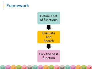
SlideShare a Scribd company logo
1 of 240
 今天的資料與投影片
1
快速上手深度學習實務
- 週末經理人研習班課程 2018/04/14
游為翔 & 周俊川
台灣人工智慧學校
Outline
 Quick review/overview
 What is Machine Learning?
 What is Deep Learning?
 Hands-on Tutorial of Deep Learning
 Training DL Models: A multi-layer perceptron example &
training tips
 Deep learning with images: Convolutional Neural Network
3
What is Machine Learning?
4
Machine Learning (ML) and Artificial Intelligence (AI)
 AI 是用電腦模擬生物智慧的一個過程或目標
 從結果來看,是否有 human intelligence
 一個擁有非常詳盡的 rule-based 系統也可以是 AI
 弱 AI ~= 專家系統 ~= 訓練有素的狗
 Machine learning 是達成 AI 的一種方法
 設計演算法與從根據問題設計特徵,並從大量數據中學
出生物智慧的 “規則”
5
Artificial
Intelligence
Machine
Learning
一句話說明 Machine Learning
6
Field of study that gives computers the ability
to learn without being explicitly programmed.
- Arthur Lee Samuel, 1959
『
』
Goal of Machine Learning
 For a specific task, find the best function to complete
 Task: 每集寶可夢結束的“猜猜我是誰”
7
f*( ) =
f*( ) =
Ans: 妙蛙種子
Ans: 超夢
Framework
8
Define a set
of functions
Evaluate
and
Search
Pick the best
function
1. Define a Set of Functions
9
Define a set
of functions
Evaluate
and
Search
Pick the best
function
A set of functions, f(‧)
{f(ө1),…,f(ө*),…,f(өn)}
在北投公園的寶可夢訓練師
2. Evaluate and Search
10
Define a set
of functions
Evaluate
and
Search
Pick the best
function
f1( ) =
f1( ) =
根據結果,修正 ө :
避免找穿黃色上衣且有皮卡丘的人 (遠離 ө1 )
f1=f(ө1)
3. Pick The Best Function
11
Define a set
of functions
Evaluate
and
Search
Pick the best
function
找到寶可夢訓練大師
Machine Learning Framework
Define a set
of functions
Evaluate
and
Search
Pick the best
function
北投公園的訓練師
評估、修正
找到最好的寶可夢專家
What is Deep Learning?
13
Deep Learning vs. Machine Learning
Deep learning is a subset of machine learning
14
Artificial Intelligence
Machine Learning
Deep Learning
人工智慧 (Artificial Intelligence) –
讓電腦 / 機器展現人類智慧
機器學習 (Machine Learning) –
達成 AI 的方法
基於下列方法
1) 大量數據
2) 人工建立的特徵
e.g. canny filter, sobel filter.
3) 事先設計好的演算法
e.g. 羅吉斯回歸, 決策樹, 隨機森林, 支持向量機
深度學習 (Deep Learning) –
模擬人類大腦神經連結建構網路
1) 可以直接使用原始資料做為輸入
2) 透過多層神經連結, 神經網路可以在訓練
的過程中自行找到輸入與輸出之關聯
Deep Learning vs. Machine Learning
Deep learning is a subset of machine learning
15
Artificial Intelligence
Machine Learning
Deep Learning
人工智慧 (Artificial Intelligence) –
讓電腦 / 機器展現人類智慧
機器學習 (Machine Learning) –
達成 AI 的方法
基於下列方法
1) 大量數據
2) 人工建立的特徵
e.g. canny filter, sobel filter.
3) 事先設計好的演算法
e.g. 羅吉斯回歸, 決策樹, 隨機森林, 支持向量機
深度學習 (Deep Learning) –
模擬人類大腦神經連結建構網路
1) 可以直接使用原始資料做為輸入
2) 透過多層神經連結, 神經網路可以在訓練
的過程中自行找到輸入與輸出之關聯
Deep Learning vs. Machine Learning
Deep learning is a subset of machine learning
16
Artificial Intelligence
Machine Learning
Deep Learning
人工智慧 (Artificial Intelligence) –
讓電腦 / 機器展現人類智慧
機器學習 (Machine Learning) –
達成 AI 的方法
基於下列方法
1) 事先設計好的演算法
e.g. 羅吉斯回歸, 決策數, 隨機森林, 支持向量機
2) 大量數據
3) 人工建立的特徵
e.g. canny filter, sobel filter.
深度學習 (Deep Learning) –
模擬人類大腦神經連結建構網路
1) 可以直接使用原始資料做為輸入
2) 透過多層神經連結, 神經網路可以在訓練
的過程中自行找到輸入與輸出之關聯
深度學習的本質: 從 A 到 B 的映射
- by Andrew Ng
Applications of Deep Learning
20
 *f
 *f
 *f
 *f
“2”
“Morning”
“5-5”
“Hello”“Hi”
(what the user said) (system response)
(step)
(Slide Credit: Hung-Yi Lee)
 Speech Recognition
 Handwritten Recognition
 Playing Go
 Dialogue System
Fundamentals of Deep Learning
 Artificial neural network (ANN, 1943)
Multi-layer perceptron
 模擬人類神經傳導機制的設計
 由許多層的 neuron 互相連結而形成 neural network
21
How neuron propagate
23
Input
x1
xn
……
z = w1x1+w2x2+……+wnxn+b
̂y
wn
w1
Output
Weight
+
z
σ: Activation
function
b
Bias
σ(z)
̂y = σ(z)
…
Neuron
How neuron propagate
 Example
24
σ(z)=z linear function
z = w1x1+w2x2+……+wnxn+b
A neuron
5
2
z = w1x1+w2x2+……+wnxn+b
3
-1
Output
+
z
σ(z)
3
̂y
̂y = z = (-1)*5+3*2+3 = 4 Ө: weights, bias
Fully Connected Neural Network
 很多個 neurons 連接成 network
 Universality theorem: a network with enough number
of neurons can present any function
25
X1
Xn
w1,n
w1,1
w2,n
w2,1
Fully Connected Neural Network -
A simple network with linear activation functions
5
2
+0.4
+0.1
+0.5
+0.9
0.12
-0.5
+0.2
-0.1
+0.5
-1.5
+0.8
0.55
PredictionForward propagation
 output values 跟 actual values 越一致越好
 A loss function is to quantify the gap between
network outputs and actual values
 Loss function is a function of Ө
如何評估模型好不好?
27
X1
X2
̂y1
̂y2
y1
y2
L
f(x,Ө)
(Ө)
Fully Connected Neural Network -
A simple network with linear activation functions
5
2
+0.4
+0.1
+0.5
+0.9
0.12
-0.5
+0.2
-0.1
+0.5
-1.5
+0.8
y1
y2
L(Ө)
0.55
Prediction Actual
Loss
Forward propagation
目標:修正𝜃, 最小化 Total Loss
 Find the best function that minimize total loss
 Find the best network weights, ө*
 𝜃∗ = argm𝑖𝑛
𝜃
𝐿(𝜃)
 最重要的問題: 該如何找到 ө* 呢?
 踏破鐵鞋無覓處 (enumerate all possible values)
 假設 weights 限制只能 0.0, 0.1, …, 0.9,有 500 個 weights
全部組合就有 10500 組
 評估 1 秒可以做 106 組,要約 10486 年
 宇宙大爆炸到現在才 1010 年
 Impossible to enumerate
29
Supplementary code
numeric_method
BP_framework
Fully Connected Neural Network -
A simple network with linear activation functions
5
2
+0.4
+0.1
+0.5
+0.9
0.12
-0.5
+0.2
-0.1
+0.5
-1.5
+0.8
y1
y2
L(Ө)
0.55
Prediction Actual
Loss
Forward propagation
Back propagation with gradient descent
Gradient Descent
 一種 heuristic 的最佳化方法,適用於連續、可微的
目標函數
 核心精神
每一步都朝著進步的方向,直到沒辦法再進步
31
當有選擇的時候,國家還是
要往進步的方向前進。
『
』http://i.imgur.com/xxzpPFN.jpg
Gradient Descent
32
L(Ө)
Ө
𝜃0
lim
Δ𝜃→0
𝐿 𝜃0 + Δ𝜃 − 𝐿(𝜃0)
𝜃0 + Δ𝜃 − 𝜃0
=
𝜕𝐿
𝜕𝜃 𝜃=𝜃0
想知道在 𝜃0
這個點時,𝐿 隨著 𝜃 的變化
𝐿 𝜃0 + Δ𝜃 − 𝐿(𝜃0)
𝜃0 + Δ𝜃 − 𝜃0
翻譯年糕:𝜃 變化一單位,會讓 𝐿 改變多少 𝑳 對 𝜽 的 gradient
(𝑡 = 0)
Δ𝜃
In this case: 𝑳 對 𝜽 的 gradient < 0
 𝜃 增加會使得 Loss 降低
 𝜃 改變的方向跟 gradient 相反
Gradient Descent
33
L(Ө)
Ө
𝜃1 = 𝜃0 − 𝜂
𝜕𝐿
𝜕𝜃 𝜃=𝜃0
𝜃0
𝝏𝑳
𝝏𝜽 𝜽=𝜽 𝟎
𝜼, Learning rate
一步要走多大
𝜃1
𝜃∗ = 𝜃 𝑛 − 𝜂
𝜕𝐿
𝜕𝜃 𝜃=𝜃 𝑛
沿著 gradient 的反方向走
𝜃∗
相信會有一天…
影響 Gradient 的因素
34
x1
xn
…… z = w1x1+w2x2+……+wnxn+b
y
wn
w1
+
z
b
σ(z)
̂y = σ(z)
̂y
L(Ө)
Ө
𝜕𝐿
𝜕𝜃
=
𝜕𝐿
𝜕 𝑦
𝜕 𝑦
𝜕𝑧
𝜕𝑧
𝜕𝜃
=
𝜕𝐿
𝜕 𝑦
𝜕 𝑦
𝜕𝜃
1. 受 loss function 影響
2. 受 activation function 影響
…
𝜃1
= 𝜃0
− 𝜂
𝜕𝐿
𝜕𝜃 𝜃=𝜃0
3. 受 learning rate 影響
Summary – Gradient Descent
 用來最佳化一個連續的目標函數
 朝著進步的方向前進
 Gradient descent
 Gradient 受 loss function 影響
 Gradient 受 activation function 影響
 受 learning rate 影響
36
Gradient Descent 的缺點
 一個 epoch 更新一次,收斂速度很慢
 一個 epoch 等於看過所有 training data 一次
 Question 1
有辦法加速嗎?
 Question 2
Gradient based method 不能保證找到全域最佳解
37
Gradient Descent 的缺點
 一個 epoch 更新一次,收斂速度很慢
 一個 epoch 等於看過所有 training data 一次
 Question 1
有辦法加速嗎?
A solution: stochastic gradient descent (SGD)
 Question 2
Gradient based method 不能保證找到全域最佳解
38
Stochastic Gradient Descent
 隨機抽一筆 training sample,依照其 loss 更新一次
 另一個問題,一筆一筆更新也很慢
 中庸之道 - Mini-batch: 每一個 mini-batch 更新一次
 Benefits of mini-batch
 相較於 SGD: faster to complete one epoch
 相較於 GD: faster to converge (to optimum)
39
Update once Update once Update once
Loss Loss Loss
Mini-batch vs. Epoch
 一個 epoch = 看完所有 training data 一次
 依照 mini-batch 把所有 training data 拆成多份
 假設全部有 1000 筆資料
 Batch size = 100 可拆成 10 份  一個 epoch 內會更新 10 次
 Batch size = 10 可拆成 100 份  一個 epoch 內會更新 100 次
 如何設定 batch size?
 不要設太大,常用 16, 32, 64, 128, 256, …
40
Gradient Descent 的缺點
 一個 epoch 更新一次,收斂速度很慢
 一個 epoch 等於看過所有 training data 一次
 Question 1
有辦法加速嗎?
A solution: stochastic gradient descent (SGD)
 Question 2
Gradient based method 不能保證找到全域最佳解
 可以利用 momentum 降低困在 local minimum 的機率
42
Momentum
43
L(Ө)
Ө
𝜃0
𝜃1
Gradient=0  不更新,陷在 local minimum
g0
m*g0
參考前一次 gradient (g0) 當作 momentum
 即使當下在 local minimum,也有機會翻過
g1=0
抵抗其運動狀態被改變的性質
Introduction of Deep Learning
 Artificial neural network
 Fully connected neural network
 Loss functions
 Gradient descent
 Loss function, activation function, learning rate
 Stochastic gradient descent
 Mini-batch
 Momentum
44
Hands-on Tutorial
An multi-layer perceptron
寶可夢雷達 using Pokemon Go Dataset on Kaggle
53
圖
範例資料
 寶可夢過去出現的時間與地點紀錄 (dataset from Kaggle)
54
Ref: https://www.kaggle.com/kostyabahshetsyan/d/semioniy/predictemall/pokemon-geolocation-visualisations/notebook
Raw Data Overview
55
問題: 會出現哪一隻神奇寶貝呢?
寶可夢雷達 Data Field Overview
 時間: local.hour, local.month, DayofWeek…
 天氣: temperature, windSpeed, pressure…
 位置: longitude, latitude, pokestop…
 環境: closeToWater, terrainType…
 十分鐘前有無出現其他寶可夢
 例如: cooc_1=1 十分鐘前出現過 class=1 之寶可夢
 class 就是我們要預測目標
56
Sampled Dataset for Fast Training
 挑選在 New York City 出現的紀錄
 挑選下列五隻常見的寶可夢
57
No.4 小火龍 No.43 走路草 No.56 猴怪 No. 71 口呆花 No.98 大鉗蟹
開始動手囉!Keras Go!
58
Input 前處理
 因為必須跟 weights 做運算
Neural network 的輸入必須為數值 (numeric)
 如何處理非數值資料?
 順序資料
 名目資料
 不同 features 的數值範圍差異會有影響嗎?
 溫度: 最低 0 度、最高 40 度
 距離: 最近 0 公尺、最遠 10000 公尺
59
處理順序資料
 Ordinal variables (順序資料)
 For example: {Low, Medium, High}
 Encoding in order
 {Low, Medium, High}  {1,2,3}
 Create a new feature using mean or median
60
UID Age
P1 0-17
P2 0-17
P3 55+
P4 26-35
UID Age
P1 15
P2 15
P3 70
P4 30
處理名目資料
 Nominal variables (名目資料)
 {"SugarFree","Half","Regular"}
 One-hot encoding
 假設有三個類別
 Category 1  [1,0,0]
 Category 2  [0,1,0]
 給予類別上的解釋  Ordinal variables
 {"SugarFree","Half","Regular"}  1,2,3
 特殊的名目資料:地址
 台北市南港區研究院路二段128號
 轉成經緯度 {25.04,121.61}
61
處理不同的數值範圍
 先說結論:建議 re-scale!但為什麼?
62
X1
X2
w1
w2
1,2,…
1000,2000,…
W2 的修正(ΔW)對於 loss 的影響比較大
y
w1
w2
w1
w2
X1
X2
w1
w2
1,2,…
1,2,…
y
Loss 等高線 Loss 等高線
處理不同的數值範圍
 影響訓練的過程
 不同 scale 的 weights 修正時會需要不同的 learning rates
 不用 adaptive learning rate 是做不好的
 在同個 scale 下,loss 的等高線會較接近圓形
 gradient 的方向會指向圓心 (最低點)
63
w1
w2
w1
w2
小提醒
 輸入 (input) 只能是數值
 名目資料、順序資料
 One-hot encoding
 順序轉成數值
 建議 re-scale 到接近的數值範圍
 今天的資料都已經先幫大家處理過了
64
Read Input File
65
import numpy as np
# 讀進檔案,以 , (逗號)分隔的 csv 檔,不包含第一行的欄位定義
my_data = np.genfromtext('pkgo_city66_class5_v1.csv',
delimiter=',',
skip_header=1)
# Input 是有 200 個欄位(index 從 0 – 199)
X_train = my_data[:,0:200]
# Output 是第 201 個欄位(index 為 200)
y_train = my_data[:,200]
# 確保資料型態正確
X_train = X_train.astype('float32')
y_train = y_train.astype('int')
Input
66
# 觀察一筆 X_train
print(X_train[1,:32])
Output 前處理
 Keras 預定的 class 數量與值有關
 挑選出的寶可夢中,最大 Pokemon ID = 98
Keras 會認為『有 99 個 classes 分別為 Class 0, 1, 2, …, 98 class』
 zero-based indexing (python)
 把下面的五隻寶可夢轉換成
67
No.4 小火龍 No.43 走路草 No.56 猴怪 No. 71 口呆花 No.98 大鉗蟹
Class 0 Class 1 Class 2 Class 3 Class 4
Output
68
# 轉換成 one-hot encoding 後的 Y_train
print(Y_train[1,:])
# [重要] 將 Output 從特定類別轉換成 one-hot encoding 的形式
from keras.utils import np_utils
Y_train = np_utils.to_categorical(y_train,5)
# 觀察一筆 y_train
print(y_train[0])
接下來的流程
 先建立一個深度學習模型
 邊移動邊開火
69
就像開始冒險前要先選一隻寶可夢
六步完模 – 建立深度學習模型
1. 決定 hidden layers 層數與其中的 neurons 數量
2. 決定每層使用的 activation function
3. 決定模型的 loss function
4. 決定 optimizer
 Parameters: learning rate, momentum, decay
5. 編譯模型 (Compile model)
6. 開始訓練囉!(Fit model)
70
步驟 1+2: 模型架構
71
from keras.models import Sequential
from keras.layers.core import Dense, Activation
from keras.optimizers import SGD
# 宣告這是一個 Sequential 次序性的深度學習模型
model = Sequential()
# 加入第一層 hidden layer (128 neurons)
# [重要] 因為第一層 hidden layer 需連接 input vector
故需要在此指定 input_dim
model.add(Dense(128, input_dim=200))
Model 建構時,是以次序性的疊加 (add) 上去
基本款 activation function
 Sigmoid function
73
步驟 1+2: 模型架構 (Cont.)
74
# 宣告這是一個 Sequential 次序性的深度學習模型
model = Sequential()
# 加入第一層 hidden layer (128 neurons) 與指定 input 的維度
model.add(Dense(128, input_dim=200))
# 指定 activation function
model.add(Activation('sigmoid'))
# 加入第二層 hidden layer (256 neurons)
model.add(Dense(256))
model.add(Activation('sigmoid'))
# 加入 output layer (5 neurons)
model.add(Dense(5))
model.add(Activation('softmax'))
# 觀察 model summary
model.summary()
Softmax
 Classification 常用 softmax 當 output 的 activation function
 Normalization: network output 轉換到[0,1] 之間且
softmax output 相加為 1  像 “機率”
 保留對其他 classes 的 prediction error
75
Output
0.6
2.6
2.2
0.1
e0.6
e2.6
e2.2
e0.1 e0.6+e2.6+e2.2+e0.1
Normalized by the sum
0.07
0.53
0.36
0.04
Exponential
Softmax
Model Summary
76
步驟 3: 選擇 loss function
 Mean_squared_error
 Mean_absolute_error
77
0.9
0.1
AnswerPrediction
0.8
0.2
(0.9 − 0.8)2+(0.1 − 0.2)2
2
= 0.01
|0.9 − 0.8| + |0.1 − 0.2|
2
= 0.1
常用於 Regression
Loss Function
 binary_crossentropy (logloss)
 categorical_crossentropy
 需要將 class 的表示方法改成 one-hot encoding
Category 1  [0,1,0,0,0]
 用簡單的函數 keras.np_utils.to_category(input)
 常用於 classification
78
−
1
𝑁
𝑛=1
𝑁
[𝑦 𝑛 log 𝑦 𝑛 + (1 − 𝑦 𝑛)log(1 − 𝑦 𝑛)]
0
1
AnswerPrediction
0.9
0.1
−
1
2
0 log 0.9 + 1 − 0 log 1 − 0.9 + 1 log 0.1 + 0 log 1 − 0.1
= −
1
2
log 0.1 + log 0.1 = − log 0.1 = 2.302585
79
0 1
1
0
80
把預測值推向兩端
降低loss
步驟 4: 選擇 optimizer
 SGD – Stochastic Gradient Descent
 Adagrad – Adaptive Learning Rate
 RMSprop – Similar with Adagrad
 Adam – Similar with RMSprop + Momentum
81
基本款 optimizer
 Stochastic gradient descent (SGD)
 設定 learning rate, momentum, learning rate decay,
Nesterov momentum
 設定 Learning rate by experiments (later)
82
# 指定 optimizier
from keras.optimizers import SGD, Adam, RMSprop, Adagrad
sgd = SGD(lr=0.01,momentum=0.0,decay=0.0,nesterov=False)
就決定是你了!
83
# 指定 loss function 和 optimizier
model.compile(loss='categorical_crossentropy',
optimizer=sgd)
Validation Dataset
 Validation dataset 用來挑選模型 (hyper-parameters)
 Testing dataset 檢驗模型的普遍性 (generalization)
避免模型過度學習 training dataset
84
Cross validation:
切出很多組的 (training, validation) 再
拿不同組訓練模型,挑選最好的模型
Testing
ValTraining
手邊收集到的資料
理論上
挑選出最好的模型後,拿
testing 檢驗 generalization
Validation Dataset
 利用 model.fit 的參數 validation_split
 從輸入 (X_train,Y_train) 取固定比例的資料作為 validation
 不會先 shuffle 再取 validation dataset
 固定從資料尾端開始取
 每個 epoch 所使用的 validation dataset 都相同
 手動加入 validation dataset
validation_data = (X_valid, Y_valid)
85
Fit Model
 batch_size: mini-batch 的大小
 nb_epoch: epoch 數量
 1 epoch 表示看過全部的 training dataset 一次
 shuffle: 每次 epoch 結束後是否要打亂 training dataset
 verbose: 是否要顯示目前的訓練進度
 0 為不顯示, 1 為正常顯示, 2 為每個 epoch 結束才顯示
86
# 指定 batch_size, nb_epoch, validation 後, 開始訓練模型!!!
history = model.fit( X_train,
Y_train,
batch_size=16,
verbose=0,
epochs=30,
shuffle=True,
validation_split=0.1)
Alternative: Functional API
 The way to go for defining a complex model
 For example: multiple outputs, multiple input source
 Why “Functional API” ?
 All layers and models are callable (like function call)
 Example
87
from keras.layers import Input, Dense
input = Input(shape=(200,))
output = Dense(10)(input)
88
# Sequential (依序的)深度學習模型
model = Sequential()
model.add(Dense(128, input_dim=200))
model.add(Activation('sigmoid'))
model.add(Dense(256))
model.add(Activation('sigmoid'))
model.add(Dense(5))
model.add(Activation('softmax'))
model.summary()
# Functional API
from keras.layers import Input, Dense
from keras.models import Model
input = Input(shape=(200,))
x = Dense(128,activation='sigmoid')(input)
x = Dense(256,activation='sigmoid')(x)
output = Dense(5,activation='softmax')(x)
# 定義 Model (function-like)
model = Model(inputs=[input], outputs=[output])
Advantages for Functional API (1)
 Model is callable as well, so it is easy to re-use the
trained model
 Re-use the architecture and weights as well
89
# If model and input is defined already
# re-use the same architecture of the above model
y1 = model(input)
Advantages for Functional API (2)
 Easy to manipulate various input sources
90
x2
Dense(100) Dense(200)y1x1 outputnew_x2
x1 = input(shape=(10,))
y1 = Dense(100)(x1)
x2 = input(shape=(20,))
new_x2 = keras.layers.concatenate([y1,x2])
output = Dense(200)(new_x2)
Model = Model(inputs=[x1,x2],outputs=[output])
Today
 Our exercise uses “Functional API” model
 Because it is more flexible than sequential model
 Ex00_first_model
91
Result
92
這樣是好是壞?
 我們選用最常見的
93
Component Selection
Loss function categorical_crossentropy
Activation function sigmoid + softmax
Optimizer SGD
用下面的招式讓模型更好吧
Tips for Training DL Models
不過盲目的使用招式,會讓你的寶可夢失去戰鬥意識
94
Tips for Deep Learning
95
No
Activation Function
YesGood result on
training dataset?
Loss Function
Good result on
testing dataset?
Optimizer
Learning Rate
Tips for Deep Learning
96
No
Activation Function
YesGood result on
training dataset?
Loss Function
Good result on
testing dataset?
Optimizer
Learning Rate
𝜕𝐿
𝜕𝜃
=
𝜕𝐿
𝜕 𝑦
𝜕 𝑦
𝜕𝑧
𝜕𝑧
𝜕𝜃
受 loss function 影響
Using MSE
 在指定 loss function 時
 ex01_lossFunc_Selection
97
# 指定 loss function 和 optimizer
model.compile(loss='categorical_crossentropy',
optimizer=sgd)
# 指定 loss function 和 optimizer
model.compile(loss='mean_squared_error',
optimizer=sgd)
Result – CE vs MSE
98
為什麼 Cross-entropy 比較好?
99
Cross-entropy
Squared error
The error surface of logarithmic functions is steeper than
that of quadratic functions. [ref]
Figure source
How to Select Loss function
 Classification 常用 cross-entropy
 搭配 softmax 當作 output layer 的 activation function
 Regression 常用 mean absolute / squared error
100
Current Best Model Configuration
101
Component Selection
Loss function categorical_crossentropy
Activation function sigmoid + softmax
Optimizer SGD
Tips for Deep Learning
102
No
Activation Function
YesGood result on
training data?
Loss Function
Good result on
testing data?
Optimizer
Learning Rate
Learning rate selection
 ex02_learningRate_Selection
103
# 指定 optimizier
from keras.optimizers import SGD, Adam, RMSprop, Adagrad
sgd = SGD(lr=0.01,momentum=0.0,decay=0.0,nesterov=False)
試試看改變 learning rate,挑選出最好的 learning rate。
建議一次降一個數量級,如: 0.1 vs 0.01 vs 0.001
Result – Learning Rate Selection
104
觀察 loss,這樣的震盪表示 learning rate 可能太大
How to Set Learning Rate
 大多要試試看才知道,通常不會大於 0.1
 一次調一個數量級
 0.1  0.01  0.001
 0.01  0.012  0.015  0.018 …
 幸運數字!
105
Tips for Deep Learning
106
No
Activation Function
YesGood result on
training data?
Loss Function
Good result on
testing data?
Optimizer
Learning Rate 𝜕𝐿
𝜕𝜃
=
𝜕𝐿
𝜕 𝑦
𝜕 𝑦
𝜕𝑧
𝜕𝑧
𝜕𝜃
受 activation function 影響
Sigmoid, Tanh, Softsign
 Sigmoid
 f(x)=
 Tanh
 f(x)=
 Softsign
 f(x)=
107
Saturation 到下一層的數值在 [-1,1] 之間
(1+e-x)
1
(1+e-2x)
(1-e-2x)
(1+|x|)
x
Derivatives of Sigmoid, Tanh, Softsign
108
gradient 小  學得慢
 Sigmoid
 df/dx=
 Tanh
 df/dx= 1-f(x)2
 Softsign
 df/dx=
(1+e-x)2
e-x
(1+|x|)2
1
Drawbacks of Sigmoid, Tanh, Softsign
 Vanishing gradient problem
 原因: input 被壓縮到一個相對很小的output range
 結果: 很大的 input 變化只能產生很小的 output 變化
 Gradient 小  無法有效地學習
 Sigmoid, Tanh, Softsign 都有這樣的特性
 特別不適用於深的深度學習模型
109
ReLU, Softplus
 ReLU
 f(x)=max(0,x)
 df/dx=
 Softplus
 f(x) = ln(1+ex)
 df/dx = ex/(1+ex)
110
1 if x > 0,
0 otherwise.
Derivatives of ReLU, Softplus
111
ReLU 在輸入小於零時, gradient 等於零,會有問題嗎?
Leaky ReLU
 Allow a small gradient while the input to activation
function smaller than 0
113
α=0.1
f(x)= x if x > 0,
αx otherwise.
df/dx=
1 if x > 0,
α otherwise.
Leaky ReLU in Keras
 更多其他的 activation functions
https://keras.io/layers/advanced-activations/
114
# For example
From keras.layer.advanced_activation import LeakyReLU
lrelu = LeakyReLU(alpha = 0.02)
model.add(Dense(128, input_dim = 200))
# 指定 activation function
model.add(lrelu)
嘗試其他的 activation functions
 ex03_activationFunction
115
# 宣告這是一個 Sequential 次序性的深度學習模型
model = Sequential()
# 加入第一層 hidden layer (128 neurons) 與指定 input 的維度
model.add(Dense(128, input_dim=200))
# 指定 activation function
model.add(Activation('relu'))
# 加入第二層 hidden layer (256 neurons)
model.add(Dense(256))
model.add(Activation('relu'))
# 加入 output layer (5 neurons)
model.add(Dense(5))
model.add(Activation('softmax'))
# 觀察 model summary
model.summary()
Result – sigmoid vs. relu vs. leaky_relu
116
How to Select Activation Functions
 Hidden layers
 通常會用 ReLU
 Sigmoid 有 vanishing gradient 的問題較不推薦
 Output layer
 Regression: linear
 Classification: softmax / sigmoid
117
Current Best Model Configuration
118
Component Selection
Loss function categorical_crossentropy
Activation function relu + softmax
Optimizer SGD
Tips for Deep Learning
119
No
YesGood result on
training dataset?
Good result on
testing dataset?
Activation Function
Loss Function
Optimizer
Learning Rate
Optimizers in Keras
 SGD – Stochastic Gradient Descent
 Adagrad – Adaptive Learning Rate
 RMSprop – Similar with Adagrad
 Adam – Similar with RMSprop + Momentum
120
Optimizer – SGD
 Stochastic gradient descent
 支援 momentum, learning rate decay, Nesterov momentum
 Momentum 的影響
 無 momentum: update = -lr*gradient
 有 momentum: update = -lr*gradient + m*last_update
 Learning rate decay after update once
 屬於 1/t decay  lr = lr / (1 + decay*t)
 t: number of done updates
121
Learning Rate with 1/t Decay
122
lr = lr / (1 + decay*t)
Momentum
 先算 gradient
 加上 momentum
 更新
Nesterov momentum
 加上 momentum
 再算 gradient
 更新
123
Nesterov Momentum
Optimizer – Adagrad
 因材施教:每個參數都有不同的 learning rate
 根據之前所有 gradient 的 root mean square 修改
124
Adaptive Learning Rate
 Feature scales 不同,需要不同的 learning rates
 每個 weight 收斂的速度不一致
 但 learning rate 沒有隨著減少的話  bumpy
 因材施教:每個參數都有不同的 learning rate
125
w1
w2
w1
w2
Optimizer – Adagrad
 根據之前所有 gradient 的 root mean square 修改
126
𝜃 𝑡+1 = 𝜃 𝑡 − 𝜂𝑔 𝑡
Gradient descent Adagrad
𝜃 𝑡+1 = 𝜃 𝑡 −
𝜂
𝜎 𝑡
𝑔 𝑡𝑔 𝑡 =
𝜕𝐿
𝜕𝜃 𝜃=𝜃 𝑡
第 t 次更新
𝜎 𝑡
=
2 (𝑔0)2+…+(𝑔 𝑡)2
𝑡 + 1
所有 gradient 的 root mean square
Step by Step – Adagrad
127
𝜃 𝑡 = 𝜃 𝑡−1 −
𝜂
𝜎 𝑡−1
𝑔 𝑡−1
𝜎 𝑡 =
(𝑔0)2+(𝑔1)2+...+(𝑔 𝑡)2
𝑡 + 1
𝜃2 = 𝜃1 −
𝜂
𝜎1
𝑔1
𝜎1 =
(𝑔0)2+(𝑔1)2
2
𝜃1 = 𝜃0 −
𝜂
𝜎0
𝑔0
𝜎0 = (𝑔0)2
 𝑔 𝑡
是一階微分,那 𝜎 𝑡
隱含什麼資訊?
An Example of Adagrad
 老馬識途,參考之前的經驗修正現在的步伐
 不完全相信當下的 gradient
 走得慢的讓他跑快點, 走的快的拉著他走慢一點
128
𝑔 𝒕
𝑔0
𝑔 𝟏
𝑔 𝟐 𝑔 𝟑
W1 0.001 0.003 0.002 0.1
W2 1.8 2.1 1.5 0.1
𝜎 𝑡
𝜎0 𝜎1 𝜎2 𝜎3
W1 0.001 0.002 0.002 0.05
W2 1.8 1.956 1.817 1.57
𝑔 𝒕/𝜎 𝑡
t=0 t=1 t=2 t=3
W1 1 1.364 0.952 2
W2 1 1.073 0.826 0.064
調整 learning rate 的 𝑔 𝒕
/𝜎 𝑡
倍
𝜃 𝑡+1
= 𝜃 𝑡
−
𝜂
(𝜎 𝑡)
𝑔 𝑡
Optimizer – RMSprop
 另一種參考過去 gradient 的方式
129
𝜎 𝑡
=
2 (𝑔0)2+…+(𝑔 𝑡)2
𝑡 + 1
Adagrad
𝜃 𝑡+1 = 𝜃 𝑡 −
𝜂
𝜎 𝑡
𝑔 𝑡
𝑟 𝑡 = (1 − 𝜌)(𝑔 𝑡)2+𝜌𝑟 𝑡−1
𝜃 𝑡+1 = 𝜃 𝑡 −
𝜂
𝑟 𝑡
𝑔 𝑡
RMSprop
Optimizer – Adam
 Close to RMSprop + Momentum
 ADAM: A Method For Stochastic Optimization
 In practice, 不改參數也會做得很好
130
比較 Optimizers
131
來源
Optimizers selection
 ex04_optimizerSelection
132
# 指定 optimizier
from keras.optimizers import SGD, Adam, RMSprop, Adagrad
sgd = SGD(lr=0.01,momentum=0.0,decay=0.0,nesterov=False)
# 指定 loss function 和 optimizier
model.compile(loss='categorical_crossentropy',
optimizer=sgd)
1. 設定選用的 optimizer
2. 修改 model compilation
Result – Adam versus SGD
133
 一般的起手式: Adam
 Adaptive learning rate for every weights
 Momentum included
134
How to Select Optimizers
Tips for Deep Learning
135
No
YesGood result on
training data?
Good result on
testing data?
Activation Function
Loss Function
Optimizer
Learning Rate
Current Best Model Configuration
136
Component Selection
Loss function categorical_crossentropy
Activation function relu + softmax
Optimizer Adam
50 epochs 後
90% 準確率!
進度報告
137
我們有90%準確率了!
但這只是在 training dataset 上的表現
這會不會只是一場美夢?
ex05_overfitCheck
見真章
138
Overfitting 啦!
Tips for Deep Learning
139
YesGood result on
training dataset?
YesGood result on
testing dataset?
No
什麼是 overfitting?
training result 進步,但 testing result 反而變差
Early Stopping
Regularization
Dropout
Batch Normalization
Tips for Deep Learning
140
YesGood result on
training dataset?
YesGood result on
testing dataset?
No
Early Stopping
Regularization
Dropout
Batch Normalization
Regularization
 限制 weights 的大小讓 output 曲線比較平滑
 為什麼要限制呢?
141
X1
X2
W1=10
W2=10
0.6
0.4
10
b=0
X1
X2
W1=1
W2=1
0.6
0.4
10
b=9
+0.1
+1 +0.1
+0.1
wi 較小  Δxi 對 ̂y 造成的影響(Δ̂y)較小
 對 input 變化比較不敏感  generalization 好
Regularization
 怎麼限制 weights 的大小呢?
加入目標函數中,一起優化
 α 是用來調整 regularization 的比重
 避免顧此失彼 (降低 weights 的大小而犧牲模型準確性)
142
Lossreg=∑(y-(b+∑wixi))
̂y
+α(regularizer)
L1 and L2 Regularizes
 L1 norm
 L2 norm
143
𝐿1 =
𝑖=1
𝑁
|𝑊𝑖|
𝐿2 =
𝑖=1
𝑁
|𝑊𝑖|2
Sum of absolute values
Root mean square of
absolute values
Regularization in Keras
144
''' Import l1,l2 (regularizer) '''
from keras.regularizers import l1,l2, l1_l2
model_l2 = Sequential()
# 加入第一層 hidden layer 並加入 regularizer (alpha=0.01)
Model_l2.add(Dense(128,input_dim=200,kernel_regularizer=l2(0.01))
Model_l2.add(Activation('relu'))
# 加入第二層 hidden layer 並加入 regularizer
model_l2.add(Dense(256, kernel_regularizer=l2(0.01)))
model_l2.add(Activation('relu'))
# 加入 Output layer
model_l2.add(Dense(5, kernel_regularizer=l2(0.01)))
model_l2.add(Activation('relu'))
Regularization in Keras
145
''' Import l1,l2 (regularizer) '''
from keras.regularizers import l1,l2,l1_l2
# 加入第一層 hidden layer 並加入 regularizer (alpha=0.01)
Model_l2.add(Dense(128,input_dim=200,kernel_regularizer=l2(0.01))
Model_l2.add(Activation('softplus'))
1. alpha = 0.01 會太大嗎?該怎麼觀察呢?
2. alpha = 0.001 再試試看
ex06_regulizers
Result – L2 Regularizer
146
Result – L2 Regularizer
147
Tips for Deep Learning
148
YesGood result on
training dataset?
YesGood result on
testing dataset?
No
Early Stopping
Regularization
Dropout
Batch Normalization
Early Stopping
 假如能早點停下來就好了…
149
Early Stopping in Keras
 Early Stopping
 monitor: 要監控的 performance index
 patience: 可以容忍連續幾次的不思長進
150
''' EarlyStopping '''
from keras.callbacks import EarlyStopping
earlyStopping=EarlyStopping(monitor = 'val_loss',
patience = 3)
ex07_earlystopping
加入 Early Stopping
151
# 指定 batch_size, nb_epoch, validation 後,開始訓練模型!!!
history = model.fit( X_train,
Y_train,
batch_size=16,
verbose=0,
epochs=30,
shuffle=True,
validation_split=0.1,
callbacks=[earlyStopping])
''' EarlyStopping '''
from keras.callbacks import EarlyStopping
earlyStopping=EarlyStopping( monitor = 'val_loss',
patience = 3)
Result – EarlyStopping (patience=3)
152
Tips for Deep Learning
153
YesGood result on
training dataset?
YesGood result on
testing dataset?
No
Early Stopping
Regularization
Dropout
Batch Normalization
Dropout
 What is Dropout?
 原本為 neurons 跟 neurons 之間為 fully connected
 在訓練過程中,隨機拿掉一些連結 (weight 設為0)
 Create multiple implicit ensembles
154
X1
Xn
w1,n
w1,1
w2,n
w2,1
Dropout 的結果
 會造成 training performance 變差
 用全部的 neurons 原本可以做到
 只用某部分的 neurons 只能做到
 Error 變大  每個 neuron 修正得越多  做得越好
155
( 𝑦 − 𝑦) < 𝜖
( 𝑦′ − 𝑦) < 𝜖 + ∆𝜖
Implications
1.
156
增加訓練的難度 在真正的考驗時爆發
2.
Dropout 2 Dropout 2NDropout 1
Dropout 可視為一種終極的 ensemble 方法
N 個 weights 會有 2N 種 network structures
Dropout in Keras
157
from keras.layers.core import Dropout
model = Sequential()
# 加入第一層 hidden layer 與 dropout=0.4
model.add(Dense(128, input_dim=200))
model.add(Activation('relu'))
model.add(Dropout(0.4))
# 加入第二層 hidden layer 與 dropout=0.4
model.add(Dense(256))
model.add(Activation('relu'))
model.add(Dropout(0.4))
# 加入 output layer (5 neurons)
model.add(Dense(5))
model.add(Activation('softmax'))
ex08_dropout
Result – Dropout or not
158
Result – Dropout or not
159
How to Set Dropout
 不要一開始就加入 Dropout
 不要一開始就加入 Dropout
不要一開始就加入 Dropout
a) Dropout 會讓 training performance 變差
b) Dropout 是在避免 overfitting,不是萬靈丹
c) 參數少時,regularization
160
Tips for Deep Learning
161
YesGood result on
training dataset?
YesGood result on
testing dataset?
No
Early Stopping
Regularization
Dropout
Batch Normalization
回顧一下
 對於 Input 的數值,前面提到建議要 re-scale
 Weights 修正的路徑比較會在同心圓山谷中往下滑
 But …, 這是只有在 inputs 啊? 如果神經網路很深, 中
間每一層的輸出會變得無法控制 (due to nonlinear
functions inside networks)
162
w1
w2
w1
w2
Loss 等高線 Loss 等高線
回顧一下
 對於 Input 的數值,前面提到建議要 re-scale
 Weights 修正的路徑比較會在同心圓山谷中往下滑
 But …, 這是只有在 inputs 啊? 如果神經網路很深, 中
間每一層的輸出會變得無法控制 (due to nonlinear
functions inside networks)
163
w1
w2
w1
w2
Loss 等高線 Loss 等高線只加在輸入層 re-scale 不夠
那你有試著每一層都 re-scale 嗎?
Batch Normalization
 每個 input feature 獨立做 normalization
 利用 batch statistics 做 normalization 而非整份資料
 同一筆資料在不同的 batch 中會有些微不同 ( a kind of
data augmentation)
164
Batch Normalization 好處多多
 可以解決 Gradient vanishing 的問題
 可以用比較大的 learning rate
 加速訓練
 取代 dropout & regularizes
 目前大多數的 Deep neural network 都會加
 大多加在 activation function 前 (Pre-activation!)
165
Comparisons
166
BN in Keras
167
from keras.layers import BatchNormalization
model = Sequential()
model.add(Dense(128, input_dim=200))
model.add(BatchNormalization())
model.add(Activation('relu'))
model.add(Dense(256))
model.add(BatchNormalization())
model.add(Activation('relu'))
# 加入 output layer (5 neurons)
model.add(Dense(5))
model.add(Activation('softmax'))
# 觀察 model summary
model.summary()
ex09_BatchNorm
Tips for Training Your Own DL Model
177
Yes Good result on
testing dataset?
No
Early Stopping
Regularization
Dropout
No
Activation Function
Loss Function
Optimizer
Learning Rate
Good result on
training dataset?
Batch Normalization
Yeah!!!
178
Variants of Deep Neural Network
Convolutional Neural Network (CNN)
179
2-dimensional Inputs
 DNN 的輸入是一維的向量,那二維的矩陣呢? 例如
圖形資料
180
Figures reference
https://twitter.com/gonainlive/status/507563446612013057
Ordinary Feedforward DNN with Image
 將圖形轉換成一維向量
 Weight 數過多,造成 training 所需時間太長
 左上的圖形跟右下的圖形真的有關係嗎?
181
300x300x3
300x300x3
1000
27 x 107
Figure reference
http://www.ettoday.net/dalemon/post/12934
Characteristics of Image
 圖的構成:線條  圖案 (pattern)物件 場景
182
Figures reference
http://www.sumiaozhijia.com/touxiang/471.html
http://122311.com/tag/su-miao/2.html
Line Segment
Pattern
Object
Scene
Patterns
 猜猜看我是誰
 辨識一個物件只需要用幾個特定圖案
183
皮卡丘 小火龍
Figures reference
http://arcadesushi.com/charmander-drunken-pokemon-tattoo/#photogallery-1=1
Why do human know that this is PICACHU
184
Patterns
 猜猜看我是誰
 甚至解析度不需要太高,有輪廓也行!
185
Property 1: What
 圖案的類型
186
皮卡丘
的耳朵
Property 2: Where
 重複的圖案可能出現在很多不同的地方
187
Figure reference
https://www.youtube.com/watch?v=NN9LaU2NlLM
Property 3: Size
 大小的變化並沒有太多影響
188
Subsampling
Feedforward DNN
CNN Structure
189
Convolutional Layer
&
Activation Layer
Pooling Layer
Can be performed
may times
Flatten
PICACHU!!!
Pooling Layer
Convolutional Layer
&
Activation Layer
New image
New image
New image
 Adding each pixel and its local neighbors which are
weighted by a filter (kernel)
 Perform this convolution process to every pixels
Convolution in Computer Vision (CV)
190
Image
Filter
How filters work?
 2 x 2 的紅色數字就是 filter
191
Intro to Convolution
 Multiply & Add
192
Figure reference
https://adeshpande3.github.io/adeshpande3.github.io/A-Beginner%27s-Guide-To-
Understanding-Convolutional-Neural-Networks/
Intro to Convolution
193
Figure reference
https://adeshpande3.github.io/adeshpande3.github.io/A-Beginner%27s-Guide-To-
Understanding-Convolutional-Neural-Networks/
6600
Intro to Convolution
194
these filters can be thought of as feature identifiers
An Example of CNN Model
195
CNN DNN
Flatten
Convolutional Layer
 Convolution 執行越多次影像越小
196
0 0 0 0 0
0 0 1 1 0
1 1 1 1 1
0 1 0 1 1
0 0 1 0 1
Image
1 2 2
1 2 3
3 1 3
New image
1 0 0
0 1 0
0 0 1
Filter
6
1 2 2
1 2 3
3 1 3
1 0 0
0 1 0
0 0 1
Layer 1
Layer 2
=*
=*
這個步驟有那些地方是可以
變化的呢?
Filter Size
 5x5 filter
197
0 0 0 0 0
0 0 1 1 0
1 1 1 1 1
0 1 0 1 1
0 0 1 0 1
Image New imageFilter
3
1 0 0 0 0
0 1 0 0 0
0 0 1 0 0
0 0 0 1 0
0 0 0 0 1
=*
1 2 2
1 2 3
3 1 3
New image
1 0 0
0 1 0
0 0 1
Filter
=
Zero-padding
 Add additional zeros at the border of image
198
0 0 0 0 0 0 0
0 0 0 0 0 0 0
0 0 0 1 1 0 0
0 1 1 1 1 1 0
0 0 1 0 1 1 0
0 0 0 1 0 1 0
0 0 0 0 0 0 0
Image
1 0 0
0 1 0
0 0 1
Filter 0 1 1 0 0
1 1 2 2 0
2 1 2 3 2
0 3 1 3 2
0 0 2 0 2
New image
=*
Zero-padding 不會影響
convolution 的性質
Stride
 Shrink the output of the convolutional layer
 Set stride as 2
199
0 0 0 0 0
0 0 1 1 0
1 1 1 1 1
0 1 0 1 1
0 0 1 0 1
Image
1 2
3 3
New image
1 0 0
0 1 0
0 0 1
Filter
=*
Convolution on RGB Image
200
0 0 1 1
1 1 1 1
0 1 0 1
0 0 1 0
0 0 1 0
1 0 1 1
0 1 0 1
1 0 1 0
0 1 0 1
1 1 0 1
0 0 0 1
0 1 1 1
RGB image
1 0 0
0 1 0
0 0 1
Filters
0 1 0
0 1 0
0 1 0
0 0 1
0 1 0
1 0 0
2 3 5 3
5 3 5 5
3 4 5 6
1 2 5 2
+
1 1 2 1
2 1 2 2
0 3 1 2
0 0 2 0
1 0 2 1
1 1 2 2
2 1 2 2
1 1 1 1
0 2 1 1
2 1 1 1
1 0 2 2
0 1 2 1
Conv. image
*
*
*
=
=
=
New image
Depth 1
201
0 1 0 1
1 1 0 1
0 0 0 1
0 1 1 1
RGB images
4x4x3
0 0 1 0
1 0 1 1
0 1 0 1
1 0 1 0
0 0 1 1
1 1 1 1
0 1 0 1
0 0 1 0
0 0 1
0 1 0
1 0 0
0 1 0
0 1 0
0 1 0
1 filter
3x3x3
1 0 0
0 1 0
0 0 1
2 3 5 3
5 3 5 5
3 4 5 6
1 2 5 2
New image
4x4x1
* =
2 3 5 3
5 3 5 5
3 4 5 6
1 2 5 2
2 3 5 3
5 3 5 2
3 4 5 1
3 4 5 2
Depth n
202
0 1 0 1
1 1 0 1
0 0 0 1
0 1 1 1
RGB images
4x4x3
0 0 1 0
1 0 1 1
0 1 0 1
1 0 1 0
0 0 1 1
1 1 1 1
0 1 0 1
0 0 1 0
0 0 1
0 1 0
1 0 0
0 1 0
0 1 0
0 1 0
n filters
n, 3x3x3
1 0 0
0 1 0
0 0 1
2 3 5 3
5 3 5 5
3 4 5 6
1 2 5 2
2 3 5 3
5 3 5 2
3 4 5 1
3 4 5 2
2 3 5 3
5 3 5 2
3 4 5 1
3 4 5 2
2 3 5 3
5 3 5 5
3 4 5 6
1 2 5 2
New image
4x4xn
0 0 1
0 1 0
1 0 0
0 1 0
0 1 0
0 1 0
1 1 0
0 1 0
1 0 1
0 0 1
0 1 0
1 0 0
0 1 0
0 1 0
0 1 0
0 0 1
0 1 0
0 0 1
n * =
如果 filters 都給定了
那 CNN 是在學什麼?
n
2 3 5 3
5 3 5 5
3 4 5 6
1 2 5 2
2 3 5 3
5 3 5 2
3 4 5 1
3 4 5 2
Depth n to Depth ?
204
2 3 5 3
5 3 5 5
3 4 5 6
1 2 5 2
2 3 5 3
5 3 5 2
3 4 5 1
3 4 5 2
2 3 5 3
5 3 5 2
3 4 5 1
3 4 5 2
9 1 4 7
4 8 5 3
3 4 1 6
1 3 0 2
4x4x?
New images 2
m * =
2 3 5 3
5 3 5 5
3 4 5 6
1 2 5 2
2 3 5 3
5 3 5 2
3 4 5 1
3 4 5 2
2 3 5 3
5 3 5 5
3 4 5 6
1 2 5 2
2 3 5 3
5 3 5 2
3 4 5 1
3 4 5 2
2 3 5 3
5 3 5 2
3 4 5 1
3 4 5 2
2 3 5 3
5 3 5 5
3 4 5 6
1 2 5 2
New images
4x4xn
0 0 1
0 1 0
1 0 0
0 1 0
0 1 0
0 1 0
Filter sets
1 0 0
0 1 0
0 0 1
1 0 0
0 1 0
0 0 1
0 0 1
0 1 0
1 0 0
0 1 0
0 1 0
0 1 0
1 0 0
0 1 0
0 0 1
1 0 0
0 1 0
0 0 1
3x3xn
Hyper-parameters of Convolutional Layer
 Filter Size
 Zero-padding
 Stride
 Depth (total number of filters)
205
An Example of CNN Model
206
256 個 filters,filter size 5x5x96
CNN DNN
Flatten
Convolution – 2D
207
The shape after convolution
 P = padding size
 S = stride
 Formula for calculating new height or width
 𝑛𝑒𝑤_ℎ𝑒𝑖𝑔ℎ𝑡 =
(𝑖𝑛𝑝𝑢𝑡_ℎ𝑒𝑖𝑔ℎ𝑡−𝑓𝑖𝑙𝑡𝑒𝑟_ℎ𝑒𝑖𝑔ℎ𝑡+2×𝑃)
𝑆
+ 1
 𝑛𝑒𝑤_𝑤𝑖𝑑𝑡ℎ =
(𝑖𝑛𝑝𝑢𝑡_𝑤𝑖𝑑𝑡ℎ−𝑓𝑖𝑙𝑡𝑒𝑟_𝑤𝑖𝑑𝑡ℎ+2×𝑃)
𝑆
+ 1
 Total number of weights is needed from 𝐿 𝑛 to 𝐿 𝑛+1
 number of filters = k
 𝑊𝑓 × 𝐻𝑓 × 𝐷 𝑛 × 𝑘 + 𝑘
208
Quiz
 parameters
 input shape = 7 x 7 x 3 (H x W x D)
 20 filters of shape = 3 x 3 x 3 (H x W x D)
 stride = 2
 no padding
 What's the shape of the output?
 Ans: 3 x 3 x 20
209
Feedforward DNN
CNN Structure
210
Convolutional Layer
&
Activation Layer
Pooling Layer
Can be performed
may times
Flatten
PICACHU!!!
Pooling Layer
Convolutional Layer
&
Activation Layer
Activation Layer
211
0 0 4 -8 0
2 0 1 1 0
1 1 1 1 1
-3 1 0 1 1
-1 0 1 -2 1
features map
σ: Activation
function
σ(features map)
0 0 4 0 0
2 0 1 1 0
1 1 1 1 1
0 1 0 1 1
0 0 1 0 1
features map
after ReLU
Feedforward DNN
CNN Structure
212
Convolutional Layer
&
Activation Layer
Pooling Layer
Can be performed
may times
Flatten
PICACHU!!!
Pooling Layer
Convolutional Layer
&
Activation Layer
Pooling Layer
 Why do we need pooling layers?
 Reduce the number of weights
 Prevent overfitting
 Max pooling
 Consider the existence of patterns in each region
213
1 2 2 0
1 2 3 2
3 1 3 2
0 2 0 2
2 3
3 3
Max pooling
*How about average pooling?
An Example of CNN Model
214
CNN DNN
Flatten
Feedforward DNN
CNN Structure
215
Convolutional Layer
&
Activation Layer
Pooling Layer
Can be performed
may times
Flatten
PICACHU!!!
Pooling Layer
Convolutional Layer
&
Activation Layer
How to connect CNN with DNN
 使用 Flatten,把影像攤平成一維的向量
216
+ +
300x300x3
270000 x 1
… +
An Example of CNN Model
 What’s the dimension after flatten?
 43,264!
217
CNN DNN
Flatten
A CNN Example (Object Recognition)
 CS231n, Stanford [Ref]
218
CNN in Keras
Object Recognition
Dataset: CIFAR-10
219
Differences between CNN and DNN
220
CNN DNN
Input Convolutional Layer
Differences between CNN and DNN
221
CNN DNN
Input Convolutional Layer
CIFAR-10 Dataset
 60,000 (50,000 training + 10,000 testing) samples,
32x32 color images in 10 classes
 10 classes
 airplane, automobile, ship, truck, bird, cat, deer, dog, frog,
horse
 Official website
 https://www.cs.toronto.edu/~kriz/cifar.html
222
Image classification
223
Overview of CIFAR-10 Dataset
 import cifar10 dataset from keras
 Files of CIFAR-10 dataset
224
CIFAR-10 Data Summary
225
How to Load CIFAR-10 Dataset by Keras
 This reading function is provided from the Keras
226
# this function is provided from the official site
from keras.datasets import cifar10
# read train/test data
(x_train, y_train), (x_test, y_test) = cifar10.load_data()
# check the data shape
print("x_train shape:", x_train.shape)
print(“y_train shape:", y_train.shape)
print("numbers of training smaples:", x_train.shape[0])
print("numbers of testing smaples:", x_test.shape[0])
Show the images
227
import matplotlib.pyplot as plt
%matplotlib inline
# show the first image of training data
plt.imshow(x_train[0])
# show the first image of testing data
plt.imshow(x_test[0])
Differences between CNN and DNN
228
CNN DNN
Input Convolutional Layer
'''CNN model'''
model = Sequential()
model.add(
Convolution2D(32, (3, 3), padding='same',
input_shape=x_train[0].shape)
)
model.add(Activation('relu'))
model.add(Convolution2D(32, (3, 3)))
model.add(Activation('relu'))
model.add(MaxPooling2D(pool_size=(2, 2)))
model.add(Dropout(0.25))
model.add(Flatten())
model.add(Dense(512))
model.add(Activation('relu'))
model.add(Dropout(0.5))
model.add(Dense(10))
model.add(Activation('softmax'))
Building Your Own CNN Model
229
32 個 3x3 filters
‘same’: perform padding
default value is zero
‘valid’ : without padding
CNN
DNN
Model Compilation
230
'''setting optimizer'''
# define the learning rate
learning_rate = 0.00017
# define the optimizer
optimizer = Adam(lr=learning_rate)
# Let’s compile
model.compile(loss='categorical_crossentropy', optimizer=
optimizer, metrics=['accuracy'])
Let’s Try CNN
 ex0_CNN_practice.ipynb
 Training time: CPU vs. GPU
 Performance: CNN vs. DNN
 Design your own CNN model (optional)
231
Figure reference
https://unsplash.com/collections/186797/coding
Tips for Setting Hyper-parameters (1)
 影像的大小須要能夠被 2 整除數次
 常見的影像 size 32, 64, 96, 224, 384, 512
 Convolutional Layer
 比起使用一個 size 較大的 filter (7x7),可以先嘗試連續使用數個 size
小的 filter (3x3)
 Stride 的值與 filter size 相關,通常 𝑠𝑡𝑟𝑖𝑑𝑒 ≤
𝑊 𝑓−1
2
 Very deep CNN model (16+ Layers) 多使用 3x3 filter 與 stride 1
232
Tips for Setting Hyper-parameters (2)
 Zero-padding 與 pooling layer 是選擇性的結構
 Zero-padding 的使用取決於是否要保留邊界的資訊
 Pooling layer 旨在避免 overfitting 與降低 weights 的數量,
但也減少影像所包含資訊,一般不會大於 3x3
 嘗試修改有不錯效能的 model,會比建立一個全新的模型容
易收斂,且 model weights 越多越難 tune 出好的參數
233
Data Augmentation
234
Why data augmentation?
 真實世界的 testing data 不一定長得跟訓練資料一樣
 避免模型 overfitting
 轉換我們手上的 training data 來增加多樣性 , 以應付未來各
種可能會出現的樣子
 Data augmentation method
 翻轉 (flip)
 平移 (shift)
 …
235
Example of data augmentation
236https://chtseng.wordpress.com/2017/11/11/data-augmentation-%E8%B3%87%E6%96%99%E5%A2%9E%E5%BC%B7/
Keras: ImageDataGenerator
237
Raw image
238http://www.sohu.com/a/208360312_717210
Width/height shift range
 ImageDataGenerator(width_shift_range=0.5,height_
shift_range=0.5)
239http://www.sohu.com/a/208360312_717210
Rotation range
 ImageDataGenerator(rotation_range=30)
240http://www.sohu.com/a/208360312_717210
Zoom range (0 < zoom_range < 1)
 ImageDataGenerator(zoom_range=0.5)
241http://www.sohu.com/a/208360312_717210
Zoom range (zoom_range >= 1)
 ImageDataGenerator(zoom_range=4)
242http://www.sohu.com/a/208360312_717210
Horizontal/Vertical flip
 ImageDataGenerator(horizontal_flip=True)
243http://www.sohu.com/a/208360312_717210
Fill mode
 ImageDataGenerator(fill_mode='wrap',
zoom_range=[4, 4])
 Fill mode: reflect, wrap, nearest, constant (cval=0)
244http://www.sohu.com/a/208360312_717210
Other Method
 Normalize method
 Featurewise_center
 Featurewise_std_normalization
 Samplewise_center
 Samplewise_std_normalization
 …
245
Keras ImageDataGenerator
 ImageDataGenerator().flow(image, batch_size)
 用 model.fit_generator 執行訓練
246
Let’s Try Data Augmentation
 ex1_CNN_data_augmentation.ipynb
 Performance: data augmentation vs. no data augmentation
 Try different data augmentation method
247
Figure reference
https://unsplash.com/collections/186797/coding
Transfer Learning
Utilize well-trained model on YOUR dataset (optional)
248
Introduction
 “transfer”: use the knowledge learned from task A to
tackle another task B
 Example: 綿羊/羊駝 classifier
249
綿羊
羊駝
其他動物的圖
Use as Fixed Feature Extractor
 A known model, like VGG, trained on ImageNet
 ImageNet: 10 millions images with labels
250
OutputInput
取某一個 layer output
當作 feature vectors
Train a classifier based on the features
extracted by a known model
Use as Initialization
 Initialize your net by the
weights of a known model
 Use your dataset to further
train your model
 Fine-tuning the known
model
251
OutputInput
OutputInput
VGG model
Your model
Intro to
 Large Scale Visual Recognition Challenge (ILSVRC)
 image classification
 1000 object classes
 1,431,167 images
252
Variety of object classes in ILSVRC
253
8 layers
19 layers
22 layers
AlexNet (2012) VGG (2014) GoogleNet (2014)
16.4%
7.3%
6.7%
http://cs231n.stanford.edu/slides/
winter1516_lecture8.pdf
Deep Neural Networks
(Slide Credit: Hung-Yi Lee)
Human yields 5.1 % error!!
AlexNet
(2012)
VGG
(2014)
GoogleNet
(2014)
152 layers
3.57%
Residual Net
(2015)
Taipei
101
101 layers
16.4%
7.3% 6.7%
Deep Neural Networks
Special
structure
Ref:
https://www.youtube.com/watch?v=
dxB6299gpvI
(Slide Credit: Hung-Yi Lee)
Human yields 5.1 % error!!
Transfer learning in Keras
256
Example of transfer learning in keras
 from keras.applications.vgg16 import VGG16
 keras.applications.vgg16.VGG16(
include_top=True, # include top layer ?
weights=‘imagenet’) # pretrained weights
 If include_top = False, input_shape could be different,
but should not too small.
257
Let’s Try Transfer learning
 ex2_CNN_transfer_learning.ipynb
 Performance: Pure CNN vs. VGG16
258
Figure reference
https://unsplash.com/collections/186797/coding
Summarization
What We Have Learned Today
259
Recap – Fundamentals
 Fundamentals of deep learning
 A neural network = a function
 Gradient descent
 Stochastic gradient descent
 Mini-batch
 Guidelines to determine a network structure
260
Recap – Improvement on Training Set
 How to improve performance on training dataset
261
Activation Function
Loss Function
Optimizer
Learning Rate
Recap – Improvement on Testing Set
 How to improve performance on testing dataset
262
Early Stopping
Regularization
Dropout
Recap – CNN
 Fundamentals of CNN
 Concept of filters
 Hyper-parameters
 Filter size
 Zero-padding
 Stride
 Depth (total number of filters)
 Pooling layers
 How to train a CNN in Keras
 CIFAR-10 dataset
263
Go Deeper in Deep Learning
 “Deep Learning”
 Written by Yoshua Bengio, Ian J. Goodfellow
 and Aaron Courville
 http://www.iro.umontreal.ca/~bengioy/dlbook/
 Course: Deep Learning Specialization (Coursera)
 Andrew NG
 https://www.coursera.org/specializations/deep-learning
 Course: Machine learning and having it deep and
structured
 http://speech.ee.ntu.edu.tw/~tlkagk/courses_MLSD15_
2.html
(Slide Credit: Hung-Yi Lee)
References
 Keras documentation Keras 官方網站,非常詳細
 Keras Github 可以從 example/ 中找到適合自己應用的範例
 Youtube 頻道 – 台大電機李宏毅教授
 Convolutional Neural Networks for Visual Recognition cs231n
 若有課程上的建議,歡迎來信
 sean@aiacademy.tw / jim@aiacademy.tw / chuan@aiacadymy.tw
 cmchang@iis.sinica.edu.tw and chihfan@iis.sinica.edu.tw
265
266
一起往訓練大師的路邁進吧!
謝謝大家!

More Related Content

What's hot

IoT GatewayとNode-REDの美味しい関係 - OpenBlocks IoTへのNode-REDの実装 -
IoT GatewayとNode-REDの美味しい関係 - OpenBlocks IoTへのNode-REDの実装 -IoT GatewayとNode-REDの美味しい関係 - OpenBlocks IoTへのNode-REDの実装 -
IoT GatewayとNode-REDの美味しい関係 - OpenBlocks IoTへのNode-REDの実装 -nodered_ug_jp
 
リクルートが実践で学んできた“セルフBI”推進に求められる3つの要素
リクルートが実践で学んできた“セルフBI”推進に求められる3つの要素リクルートが実践で学んできた“セルフBI”推進に求められる3つの要素
リクルートが実践で学んできた“セルフBI”推進に求められる3つの要素Recruit Technologies
 
Kubernetesを使う上で抑えておくべきAWSの基礎概念
Kubernetesを使う上で抑えておくべきAWSの基礎概念Kubernetesを使う上で抑えておくべきAWSの基礎概念
Kubernetesを使う上で抑えておくべきAWSの基礎概念Shinya Mori (@mosuke5)
 
[DeepLearning論文読み会] Dataset Distillation
[DeepLearning論文読み会] Dataset Distillation[DeepLearning論文読み会] Dataset Distillation
[DeepLearning論文読み会] Dataset DistillationRyutaro Yamauchi
 
ROSによる今後のロボティクスのあり方
ROSによる今後のロボティクスのあり方ROSによる今後のロボティクスのあり方
ROSによる今後のロボティクスのあり方Mori Ken
 
インターネットの仕組みとISPの構造
インターネットの仕組みとISPの構造インターネットの仕組みとISPの構造
インターネットの仕組みとISPの構造Taiji Tsuchiya
 
WSDM2018 読み会 Latent cross making use of context in recurrent recommender syst...
WSDM2018 読み会 Latent cross making use of context in recurrent recommender syst...WSDM2018 読み会 Latent cross making use of context in recurrent recommender syst...
WSDM2018 読み会 Latent cross making use of context in recurrent recommender syst...Takanori Nakai
 
ChatGPTの仕組みの解説と実務でのLLMの適用の紹介_latest.pdf
ChatGPTの仕組みの解説と実務でのLLMの適用の紹介_latest.pdfChatGPTの仕組みの解説と実務でのLLMの適用の紹介_latest.pdf
ChatGPTの仕組みの解説と実務でのLLMの適用の紹介_latest.pdfGinpei Kobayashi
 
Unboundの最適化(OSC2011 Tokyo/Spring)
Unboundの最適化(OSC2011 Tokyo/Spring)Unboundの最適化(OSC2011 Tokyo/Spring)
Unboundの最適化(OSC2011 Tokyo/Spring)Takashi Takizawa
 
モデル高速化百選
モデル高速化百選モデル高速化百選
モデル高速化百選Yusuke Uchida
 
HELLO AI WORLD - MEET JETSON NANO
HELLO AI WORLD - MEET JETSON NANOHELLO AI WORLD - MEET JETSON NANO
HELLO AI WORLD - MEET JETSON NANONVIDIA Japan
 
IPv6って何?(拡張ヘッダ編)
IPv6って何?(拡張ヘッダ編)IPv6って何?(拡張ヘッダ編)
IPv6って何?(拡張ヘッダ編)nemumu
 
PDFのコピペが文字化けするのはなぜか?~CID/GIDと原ノ味フォント~
PDFのコピペが文字化けするのはなぜか?~CID/GIDと原ノ味フォント~PDFのコピペが文字化けするのはなぜか?~CID/GIDと原ノ味フォント~
PDFのコピペが文字化けするのはなぜか?~CID/GIDと原ノ味フォント~Masamichi Hosoda
 
【DL輪読会】DINOv2: Learning Robust Visual Features without Supervision
【DL輪読会】DINOv2: Learning Robust Visual Features without Supervision【DL輪読会】DINOv2: Learning Robust Visual Features without Supervision
【DL輪読会】DINOv2: Learning Robust Visual Features without SupervisionDeep Learning JP
 
コンピュータビジョンの研究開発状況
コンピュータビジョンの研究開発状況コンピュータビジョンの研究開発状況
コンピュータビジョンの研究開発状況cvpaper. challenge
 
【LT資料】 Neural Network 素人なんだけど何とかご機嫌取りをしたい
【LT資料】 Neural Network 素人なんだけど何とかご機嫌取りをしたい【LT資料】 Neural Network 素人なんだけど何とかご機嫌取りをしたい
【LT資料】 Neural Network 素人なんだけど何とかご機嫌取りをしたいTakuji Tahara
 
[DL輪読会]BERT: Pre-training of Deep Bidirectional Transformers for Language Und...
[DL輪読会]BERT: Pre-training of Deep Bidirectional Transformers for Language Und...[DL輪読会]BERT: Pre-training of Deep Bidirectional Transformers for Language Und...
[DL輪読会]BERT: Pre-training of Deep Bidirectional Transformers for Language Und...Deep Learning JP
 
KLabのエンジニアを支えるカルチャー
KLabのエンジニアを支えるカルチャーKLabのエンジニアを支えるカルチャー
KLabのエンジニアを支えるカルチャーKLab Inc. / Tech
 
人と人の相性を考慮したシフトスケジューラ
人と人の相性を考慮したシフトスケジューラ人と人の相性を考慮したシフトスケジューラ
人と人の相性を考慮したシフトスケジューラ鈴木 庸氏
 

What's hot (20)

IoT GatewayとNode-REDの美味しい関係 - OpenBlocks IoTへのNode-REDの実装 -
IoT GatewayとNode-REDの美味しい関係 - OpenBlocks IoTへのNode-REDの実装 -IoT GatewayとNode-REDの美味しい関係 - OpenBlocks IoTへのNode-REDの実装 -
IoT GatewayとNode-REDの美味しい関係 - OpenBlocks IoTへのNode-REDの実装 -
 
リクルートが実践で学んできた“セルフBI”推進に求められる3つの要素
リクルートが実践で学んできた“セルフBI”推進に求められる3つの要素リクルートが実践で学んできた“セルフBI”推進に求められる3つの要素
リクルートが実践で学んできた“セルフBI”推進に求められる3つの要素
 
Kubernetesを使う上で抑えておくべきAWSの基礎概念
Kubernetesを使う上で抑えておくべきAWSの基礎概念Kubernetesを使う上で抑えておくべきAWSの基礎概念
Kubernetesを使う上で抑えておくべきAWSの基礎概念
 
[DeepLearning論文読み会] Dataset Distillation
[DeepLearning論文読み会] Dataset Distillation[DeepLearning論文読み会] Dataset Distillation
[DeepLearning論文読み会] Dataset Distillation
 
ROSによる今後のロボティクスのあり方
ROSによる今後のロボティクスのあり方ROSによる今後のロボティクスのあり方
ROSによる今後のロボティクスのあり方
 
インターネットの仕組みとISPの構造
インターネットの仕組みとISPの構造インターネットの仕組みとISPの構造
インターネットの仕組みとISPの構造
 
WSDM2018 読み会 Latent cross making use of context in recurrent recommender syst...
WSDM2018 読み会 Latent cross making use of context in recurrent recommender syst...WSDM2018 読み会 Latent cross making use of context in recurrent recommender syst...
WSDM2018 読み会 Latent cross making use of context in recurrent recommender syst...
 
ChatGPTの仕組みの解説と実務でのLLMの適用の紹介_latest.pdf
ChatGPTの仕組みの解説と実務でのLLMの適用の紹介_latest.pdfChatGPTの仕組みの解説と実務でのLLMの適用の紹介_latest.pdf
ChatGPTの仕組みの解説と実務でのLLMの適用の紹介_latest.pdf
 
Unboundの最適化(OSC2011 Tokyo/Spring)
Unboundの最適化(OSC2011 Tokyo/Spring)Unboundの最適化(OSC2011 Tokyo/Spring)
Unboundの最適化(OSC2011 Tokyo/Spring)
 
モデル高速化百選
モデル高速化百選モデル高速化百選
モデル高速化百選
 
HELLO AI WORLD - MEET JETSON NANO
HELLO AI WORLD - MEET JETSON NANOHELLO AI WORLD - MEET JETSON NANO
HELLO AI WORLD - MEET JETSON NANO
 
IPv6って何?(拡張ヘッダ編)
IPv6って何?(拡張ヘッダ編)IPv6って何?(拡張ヘッダ編)
IPv6って何?(拡張ヘッダ編)
 
PDFのコピペが文字化けするのはなぜか?~CID/GIDと原ノ味フォント~
PDFのコピペが文字化けするのはなぜか?~CID/GIDと原ノ味フォント~PDFのコピペが文字化けするのはなぜか?~CID/GIDと原ノ味フォント~
PDFのコピペが文字化けするのはなぜか?~CID/GIDと原ノ味フォント~
 
【DL輪読会】DINOv2: Learning Robust Visual Features without Supervision
【DL輪読会】DINOv2: Learning Robust Visual Features without Supervision【DL輪読会】DINOv2: Learning Robust Visual Features without Supervision
【DL輪読会】DINOv2: Learning Robust Visual Features without Supervision
 
コンピュータビジョンの研究開発状況
コンピュータビジョンの研究開発状況コンピュータビジョンの研究開発状況
コンピュータビジョンの研究開発状況
 
Jsai
JsaiJsai
Jsai
 
【LT資料】 Neural Network 素人なんだけど何とかご機嫌取りをしたい
【LT資料】 Neural Network 素人なんだけど何とかご機嫌取りをしたい【LT資料】 Neural Network 素人なんだけど何とかご機嫌取りをしたい
【LT資料】 Neural Network 素人なんだけど何とかご機嫌取りをしたい
 
[DL輪読会]BERT: Pre-training of Deep Bidirectional Transformers for Language Und...
[DL輪読会]BERT: Pre-training of Deep Bidirectional Transformers for Language Und...[DL輪読会]BERT: Pre-training of Deep Bidirectional Transformers for Language Und...
[DL輪読会]BERT: Pre-training of Deep Bidirectional Transformers for Language Und...
 
KLabのエンジニアを支えるカルチャー
KLabのエンジニアを支えるカルチャーKLabのエンジニアを支えるカルチャー
KLabのエンジニアを支えるカルチャー
 
人と人の相性を考慮したシフトスケジューラ
人と人の相性を考慮したシフトスケジューラ人と人の相性を考慮したシフトスケジューラ
人と人の相性を考慮したシフトスケジューラ
 

Similar to Baisc Deep Learning HandsOn

Deep Learning with Apache MXNet (September 2017)
Deep Learning with Apache MXNet (September 2017)Deep Learning with Apache MXNet (September 2017)
Deep Learning with Apache MXNet (September 2017)Julien SIMON
 
[系列活動] 手把手的深度學習實務
[系列活動] 手把手的深度學習實務[系列活動] 手把手的深度學習實務
[系列活動] 手把手的深度學習實務台灣資料科學年會
 
Hands-on Tutorial of Deep Learning
Hands-on Tutorial of Deep LearningHands-on Tutorial of Deep Learning
Hands-on Tutorial of Deep LearningChun-Ming Chang
 
An Introduction to Deep Learning (May 2018)
An Introduction to Deep Learning (May 2018)An Introduction to Deep Learning (May 2018)
An Introduction to Deep Learning (May 2018)Julien SIMON
 
Deep Learning for Developers
Deep Learning for DevelopersDeep Learning for Developers
Deep Learning for DevelopersJulien SIMON
 
Deep Learning for Developers (Advanced Workshop)
Deep Learning for Developers (Advanced Workshop)Deep Learning for Developers (Advanced Workshop)
Deep Learning for Developers (Advanced Workshop)Amazon Web Services
 
Deep Dive on Deep Learning (June 2018)
Deep Dive on Deep Learning (June 2018)Deep Dive on Deep Learning (June 2018)
Deep Dive on Deep Learning (June 2018)Julien SIMON
 
Separating Hype from Reality in Deep Learning with Sameer Farooqui
 Separating Hype from Reality in Deep Learning with Sameer Farooqui Separating Hype from Reality in Deep Learning with Sameer Farooqui
Separating Hype from Reality in Deep Learning with Sameer FarooquiDatabricks
 
[系列活動] 手把手的深度學實務
[系列活動] 手把手的深度學實務[系列活動] 手把手的深度學實務
[系列活動] 手把手的深度學實務台灣資料科學年會
 
Neural Networks in the Wild: Handwriting Recognition
Neural Networks in the Wild: Handwriting RecognitionNeural Networks in the Wild: Handwriting Recognition
Neural Networks in the Wild: Handwriting RecognitionJohn Liu
 
[DSC Adria 23]Danko_Nikolic - Guided Transfer Learning.pptx
[DSC Adria 23]Danko_Nikolic - Guided Transfer Learning.pptx[DSC Adria 23]Danko_Nikolic - Guided Transfer Learning.pptx
[DSC Adria 23]Danko_Nikolic - Guided Transfer Learning.pptxDataScienceConferenc1
 
Deep Learning - The Past, Present and Future of Artificial Intelligence
Deep Learning - The Past, Present and Future of Artificial IntelligenceDeep Learning - The Past, Present and Future of Artificial Intelligence
Deep Learning - The Past, Present and Future of Artificial IntelligenceLukas Masuch
 
Convolutional neural network
Convolutional neural networkConvolutional neural network
Convolutional neural networkItachi SK
 
Artificial Neural Networks-Supervised Learning Models
Artificial Neural Networks-Supervised Learning ModelsArtificial Neural Networks-Supervised Learning Models
Artificial Neural Networks-Supervised Learning ModelsDrBaljitSinghKhehra
 
Artificial Neural Networks-Supervised Learning Models
Artificial Neural Networks-Supervised Learning ModelsArtificial Neural Networks-Supervised Learning Models
Artificial Neural Networks-Supervised Learning ModelsDrBaljitSinghKhehra
 
Artificial Neural Networks-Supervised Learning Models
Artificial Neural Networks-Supervised Learning ModelsArtificial Neural Networks-Supervised Learning Models
Artificial Neural Networks-Supervised Learning ModelsDrBaljitSinghKhehra
 
Deep Learning And Business Models (VNITC 2015-09-13)
Deep Learning And Business Models (VNITC 2015-09-13)Deep Learning And Business Models (VNITC 2015-09-13)
Deep Learning And Business Models (VNITC 2015-09-13)Ha Phuong
 
Ai demystified (dbe, south campus)
Ai  demystified (dbe, south campus)Ai  demystified (dbe, south campus)
Ai demystified (dbe, south campus)SaurabhKhanna31
 

Similar to Baisc Deep Learning HandsOn (20)

Deep Learning with Apache MXNet (September 2017)
Deep Learning with Apache MXNet (September 2017)Deep Learning with Apache MXNet (September 2017)
Deep Learning with Apache MXNet (September 2017)
 
[系列活動] 手把手的深度學習實務
[系列活動] 手把手的深度學習實務[系列活動] 手把手的深度學習實務
[系列活動] 手把手的深度學習實務
 
Hands-on Tutorial of Deep Learning
Hands-on Tutorial of Deep LearningHands-on Tutorial of Deep Learning
Hands-on Tutorial of Deep Learning
 
An Introduction to Deep Learning (May 2018)
An Introduction to Deep Learning (May 2018)An Introduction to Deep Learning (May 2018)
An Introduction to Deep Learning (May 2018)
 
Deep Learning for Developers
Deep Learning for DevelopersDeep Learning for Developers
Deep Learning for Developers
 
Deep Learning for Developers (Advanced Workshop)
Deep Learning for Developers (Advanced Workshop)Deep Learning for Developers (Advanced Workshop)
Deep Learning for Developers (Advanced Workshop)
 
Deep Dive on Deep Learning (June 2018)
Deep Dive on Deep Learning (June 2018)Deep Dive on Deep Learning (June 2018)
Deep Dive on Deep Learning (June 2018)
 
AI and Deep Learning
AI and Deep Learning AI and Deep Learning
AI and Deep Learning
 
Separating Hype from Reality in Deep Learning with Sameer Farooqui
 Separating Hype from Reality in Deep Learning with Sameer Farooqui Separating Hype from Reality in Deep Learning with Sameer Farooqui
Separating Hype from Reality in Deep Learning with Sameer Farooqui
 
[系列活動] 手把手的深度學實務
[系列活動] 手把手的深度學實務[系列活動] 手把手的深度學實務
[系列活動] 手把手的深度學實務
 
Neural Networks in the Wild: Handwriting Recognition
Neural Networks in the Wild: Handwriting RecognitionNeural Networks in the Wild: Handwriting Recognition
Neural Networks in the Wild: Handwriting Recognition
 
[DSC Adria 23]Danko_Nikolic - Guided Transfer Learning.pptx
[DSC Adria 23]Danko_Nikolic - Guided Transfer Learning.pptx[DSC Adria 23]Danko_Nikolic - Guided Transfer Learning.pptx
[DSC Adria 23]Danko_Nikolic - Guided Transfer Learning.pptx
 
Artificial Neural networks
Artificial Neural networksArtificial Neural networks
Artificial Neural networks
 
Deep Learning - The Past, Present and Future of Artificial Intelligence
Deep Learning - The Past, Present and Future of Artificial IntelligenceDeep Learning - The Past, Present and Future of Artificial Intelligence
Deep Learning - The Past, Present and Future of Artificial Intelligence
 
Convolutional neural network
Convolutional neural networkConvolutional neural network
Convolutional neural network
 
Artificial Neural Networks-Supervised Learning Models
Artificial Neural Networks-Supervised Learning ModelsArtificial Neural Networks-Supervised Learning Models
Artificial Neural Networks-Supervised Learning Models
 
Artificial Neural Networks-Supervised Learning Models
Artificial Neural Networks-Supervised Learning ModelsArtificial Neural Networks-Supervised Learning Models
Artificial Neural Networks-Supervised Learning Models
 
Artificial Neural Networks-Supervised Learning Models
Artificial Neural Networks-Supervised Learning ModelsArtificial Neural Networks-Supervised Learning Models
Artificial Neural Networks-Supervised Learning Models
 
Deep Learning And Business Models (VNITC 2015-09-13)
Deep Learning And Business Models (VNITC 2015-09-13)Deep Learning And Business Models (VNITC 2015-09-13)
Deep Learning And Business Models (VNITC 2015-09-13)
 
Ai demystified (dbe, south campus)
Ai  demystified (dbe, south campus)Ai  demystified (dbe, south campus)
Ai demystified (dbe, south campus)
 

More from Sean Yu

AI-powered Medical Imaging Analysis for Precision Medicine
AI-powered Medical Imaging Analysis for Precision MedicineAI-powered Medical Imaging Analysis for Precision Medicine
AI-powered Medical Imaging Analysis for Precision MedicineSean Yu
 
Weakly Supervised Whole Slide Image Analysis Using Cloud Computing
Weakly Supervised Whole Slide Image Analysis Using Cloud ComputingWeakly Supervised Whole Slide Image Analysis Using Cloud Computing
Weakly Supervised Whole Slide Image Analysis Using Cloud ComputingSean Yu
 
NTU DBME5028 Week8 Transfer Learning
NTU DBME5028 Week8 Transfer LearningNTU DBME5028 Week8 Transfer Learning
NTU DBME5028 Week8 Transfer LearningSean Yu
 
NTU DBME5028 Week5 Introduction to Machine Learning
NTU DBME5028 Week5 Introduction to Machine Learning NTU DBME5028 Week5 Introduction to Machine Learning
NTU DBME5028 Week5 Introduction to Machine Learning Sean Yu
 
Practical aspects of medical image ai for hospital (IRB course)
Practical aspects of medical image ai for hospital (IRB course)Practical aspects of medical image ai for hospital (IRB course)
Practical aspects of medical image ai for hospital (IRB course)Sean Yu
 
[Taiwan AI Academy] Machine learning and deep learning application examples
[Taiwan AI Academy] Machine learning and deep learning application examples[Taiwan AI Academy] Machine learning and deep learning application examples
[Taiwan AI Academy] Machine learning and deep learning application examplesSean Yu
 
[Python - Deep Learning] Data generator
[Python - Deep Learning] Data generator[Python - Deep Learning] Data generator
[Python - Deep Learning] Data generatorSean Yu
 
日常生活中的機器學習與 AI 應用 - 院區公開演講
日常生活中的機器學習與 AI 應用 - 院區公開演講日常生活中的機器學習與 AI 應用 - 院區公開演講
日常生活中的機器學習與 AI 應用 - 院區公開演講Sean Yu
 
台灣人工智慧年會 - 兩位跨領域者的深度學習之旅
台灣人工智慧年會 - 兩位跨領域者的深度學習之旅台灣人工智慧年會 - 兩位跨領域者的深度學習之旅
台灣人工智慧年會 - 兩位跨領域者的深度學習之旅Sean Yu
 
R 語言教學: 探索性資料分析與文字探勘初探
R 語言教學: 探索性資料分析與文字探勘初探R 語言教學: 探索性資料分析與文字探勘初探
R 語言教學: 探索性資料分析與文字探勘初探Sean Yu
 

More from Sean Yu (10)

AI-powered Medical Imaging Analysis for Precision Medicine
AI-powered Medical Imaging Analysis for Precision MedicineAI-powered Medical Imaging Analysis for Precision Medicine
AI-powered Medical Imaging Analysis for Precision Medicine
 
Weakly Supervised Whole Slide Image Analysis Using Cloud Computing
Weakly Supervised Whole Slide Image Analysis Using Cloud ComputingWeakly Supervised Whole Slide Image Analysis Using Cloud Computing
Weakly Supervised Whole Slide Image Analysis Using Cloud Computing
 
NTU DBME5028 Week8 Transfer Learning
NTU DBME5028 Week8 Transfer LearningNTU DBME5028 Week8 Transfer Learning
NTU DBME5028 Week8 Transfer Learning
 
NTU DBME5028 Week5 Introduction to Machine Learning
NTU DBME5028 Week5 Introduction to Machine Learning NTU DBME5028 Week5 Introduction to Machine Learning
NTU DBME5028 Week5 Introduction to Machine Learning
 
Practical aspects of medical image ai for hospital (IRB course)
Practical aspects of medical image ai for hospital (IRB course)Practical aspects of medical image ai for hospital (IRB course)
Practical aspects of medical image ai for hospital (IRB course)
 
[Taiwan AI Academy] Machine learning and deep learning application examples
[Taiwan AI Academy] Machine learning and deep learning application examples[Taiwan AI Academy] Machine learning and deep learning application examples
[Taiwan AI Academy] Machine learning and deep learning application examples
 
[Python - Deep Learning] Data generator
[Python - Deep Learning] Data generator[Python - Deep Learning] Data generator
[Python - Deep Learning] Data generator
 
日常生活中的機器學習與 AI 應用 - 院區公開演講
日常生活中的機器學習與 AI 應用 - 院區公開演講日常生活中的機器學習與 AI 應用 - 院區公開演講
日常生活中的機器學習與 AI 應用 - 院區公開演講
 
台灣人工智慧年會 - 兩位跨領域者的深度學習之旅
台灣人工智慧年會 - 兩位跨領域者的深度學習之旅台灣人工智慧年會 - 兩位跨領域者的深度學習之旅
台灣人工智慧年會 - 兩位跨領域者的深度學習之旅
 
R 語言教學: 探索性資料分析與文字探勘初探
R 語言教學: 探索性資料分析與文字探勘初探R 語言教學: 探索性資料分析與文字探勘初探
R 語言教學: 探索性資料分析與文字探勘初探
 

Recently uploaded

Indian Call Girls in Abu Dhabi O5286O24O8 Call Girls in Abu Dhabi By Independ...
Indian Call Girls in Abu Dhabi O5286O24O8 Call Girls in Abu Dhabi By Independ...Indian Call Girls in Abu Dhabi O5286O24O8 Call Girls in Abu Dhabi By Independ...
Indian Call Girls in Abu Dhabi O5286O24O8 Call Girls in Abu Dhabi By Independ...dajasot375
 
Unveiling Insights: The Role of a Data Analyst
Unveiling Insights: The Role of a Data AnalystUnveiling Insights: The Role of a Data Analyst
Unveiling Insights: The Role of a Data AnalystSamantha Rae Coolbeth
 
Beautiful Sapna Vip Call Girls Hauz Khas 9711199012 Call /Whatsapps
Beautiful Sapna Vip  Call Girls Hauz Khas 9711199012 Call /WhatsappsBeautiful Sapna Vip  Call Girls Hauz Khas 9711199012 Call /Whatsapps
Beautiful Sapna Vip Call Girls Hauz Khas 9711199012 Call /Whatsappssapnasaifi408
 
Building on a FAIRly Strong Foundation to Connect Academic Research to Transl...
Building on a FAIRly Strong Foundation to Connect Academic Research to Transl...Building on a FAIRly Strong Foundation to Connect Academic Research to Transl...
Building on a FAIRly Strong Foundation to Connect Academic Research to Transl...Jack DiGiovanna
 
Aminabad Call Girl Agent 9548273370 , Call Girls Service Lucknow
Aminabad Call Girl Agent 9548273370 , Call Girls Service LucknowAminabad Call Girl Agent 9548273370 , Call Girls Service Lucknow
Aminabad Call Girl Agent 9548273370 , Call Girls Service Lucknowmakika9823
 
Saket, (-DELHI )+91-9654467111-(=)CHEAP Call Girls in Escorts Service Saket C...
Saket, (-DELHI )+91-9654467111-(=)CHEAP Call Girls in Escorts Service Saket C...Saket, (-DELHI )+91-9654467111-(=)CHEAP Call Girls in Escorts Service Saket C...
Saket, (-DELHI )+91-9654467111-(=)CHEAP Call Girls in Escorts Service Saket C...Sapana Sha
 
VIP High Class Call Girls Bikaner Anushka 8250192130 Independent Escort Servi...
VIP High Class Call Girls Bikaner Anushka 8250192130 Independent Escort Servi...VIP High Class Call Girls Bikaner Anushka 8250192130 Independent Escort Servi...
VIP High Class Call Girls Bikaner Anushka 8250192130 Independent Escort Servi...Suhani Kapoor
 
Digi Khata Problem along complete plan.pptx
Digi Khata Problem along complete plan.pptxDigi Khata Problem along complete plan.pptx
Digi Khata Problem along complete plan.pptxTanveerAhmed817946
 
(PARI) Call Girls Wanowrie ( 7001035870 ) HI-Fi Pune Escorts Service
(PARI) Call Girls Wanowrie ( 7001035870 ) HI-Fi Pune Escorts Service(PARI) Call Girls Wanowrie ( 7001035870 ) HI-Fi Pune Escorts Service
(PARI) Call Girls Wanowrie ( 7001035870 ) HI-Fi Pune Escorts Serviceranjana rawat
 
100-Concepts-of-AI by Anupama Kate .pptx
100-Concepts-of-AI by Anupama Kate .pptx100-Concepts-of-AI by Anupama Kate .pptx
100-Concepts-of-AI by Anupama Kate .pptxAnupama Kate
 
Call Girls in Defence Colony Delhi 💯Call Us 🔝8264348440🔝
Call Girls in Defence Colony Delhi 💯Call Us 🔝8264348440🔝Call Girls in Defence Colony Delhi 💯Call Us 🔝8264348440🔝
Call Girls in Defence Colony Delhi 💯Call Us 🔝8264348440🔝soniya singh
 
FESE Capital Markets Fact Sheet 2024 Q1.pdf
FESE Capital Markets Fact Sheet 2024 Q1.pdfFESE Capital Markets Fact Sheet 2024 Q1.pdf
FESE Capital Markets Fact Sheet 2024 Q1.pdfMarinCaroMartnezBerg
 
Call Girls In Mahipalpur O9654467111 Escorts Service
Call Girls In Mahipalpur O9654467111  Escorts ServiceCall Girls In Mahipalpur O9654467111  Escorts Service
Call Girls In Mahipalpur O9654467111 Escorts ServiceSapana Sha
 
Predicting Employee Churn: A Data-Driven Approach Project Presentation
Predicting Employee Churn: A Data-Driven Approach Project PresentationPredicting Employee Churn: A Data-Driven Approach Project Presentation
Predicting Employee Churn: A Data-Driven Approach Project PresentationBoston Institute of Analytics
 
VIP Call Girls Service Miyapur Hyderabad Call +91-8250192130
VIP Call Girls Service Miyapur Hyderabad Call +91-8250192130VIP Call Girls Service Miyapur Hyderabad Call +91-8250192130
VIP Call Girls Service Miyapur Hyderabad Call +91-8250192130Suhani Kapoor
 
EMERCE - 2024 - AMSTERDAM - CROSS-PLATFORM TRACKING WITH GOOGLE ANALYTICS.pptx
EMERCE - 2024 - AMSTERDAM - CROSS-PLATFORM  TRACKING WITH GOOGLE ANALYTICS.pptxEMERCE - 2024 - AMSTERDAM - CROSS-PLATFORM  TRACKING WITH GOOGLE ANALYTICS.pptx
EMERCE - 2024 - AMSTERDAM - CROSS-PLATFORM TRACKING WITH GOOGLE ANALYTICS.pptxthyngster
 

Recently uploaded (20)

Indian Call Girls in Abu Dhabi O5286O24O8 Call Girls in Abu Dhabi By Independ...
Indian Call Girls in Abu Dhabi O5286O24O8 Call Girls in Abu Dhabi By Independ...Indian Call Girls in Abu Dhabi O5286O24O8 Call Girls in Abu Dhabi By Independ...
Indian Call Girls in Abu Dhabi O5286O24O8 Call Girls in Abu Dhabi By Independ...
 
Decoding Loan Approval: Predictive Modeling in Action
Decoding Loan Approval: Predictive Modeling in ActionDecoding Loan Approval: Predictive Modeling in Action
Decoding Loan Approval: Predictive Modeling in Action
 
Unveiling Insights: The Role of a Data Analyst
Unveiling Insights: The Role of a Data AnalystUnveiling Insights: The Role of a Data Analyst
Unveiling Insights: The Role of a Data Analyst
 
VIP Call Girls Service Charbagh { Lucknow Call Girls Service 9548273370 } Boo...
VIP Call Girls Service Charbagh { Lucknow Call Girls Service 9548273370 } Boo...VIP Call Girls Service Charbagh { Lucknow Call Girls Service 9548273370 } Boo...
VIP Call Girls Service Charbagh { Lucknow Call Girls Service 9548273370 } Boo...
 
Beautiful Sapna Vip Call Girls Hauz Khas 9711199012 Call /Whatsapps
Beautiful Sapna Vip  Call Girls Hauz Khas 9711199012 Call /WhatsappsBeautiful Sapna Vip  Call Girls Hauz Khas 9711199012 Call /Whatsapps
Beautiful Sapna Vip Call Girls Hauz Khas 9711199012 Call /Whatsapps
 
Delhi 99530 vip 56974 Genuine Escort Service Call Girls in Kishangarh
Delhi 99530 vip 56974 Genuine Escort Service Call Girls in  KishangarhDelhi 99530 vip 56974 Genuine Escort Service Call Girls in  Kishangarh
Delhi 99530 vip 56974 Genuine Escort Service Call Girls in Kishangarh
 
Building on a FAIRly Strong Foundation to Connect Academic Research to Transl...
Building on a FAIRly Strong Foundation to Connect Academic Research to Transl...Building on a FAIRly Strong Foundation to Connect Academic Research to Transl...
Building on a FAIRly Strong Foundation to Connect Academic Research to Transl...
 
Aminabad Call Girl Agent 9548273370 , Call Girls Service Lucknow
Aminabad Call Girl Agent 9548273370 , Call Girls Service LucknowAminabad Call Girl Agent 9548273370 , Call Girls Service Lucknow
Aminabad Call Girl Agent 9548273370 , Call Girls Service Lucknow
 
E-Commerce Order PredictionShraddha Kamble.pptx
E-Commerce Order PredictionShraddha Kamble.pptxE-Commerce Order PredictionShraddha Kamble.pptx
E-Commerce Order PredictionShraddha Kamble.pptx
 
Saket, (-DELHI )+91-9654467111-(=)CHEAP Call Girls in Escorts Service Saket C...
Saket, (-DELHI )+91-9654467111-(=)CHEAP Call Girls in Escorts Service Saket C...Saket, (-DELHI )+91-9654467111-(=)CHEAP Call Girls in Escorts Service Saket C...
Saket, (-DELHI )+91-9654467111-(=)CHEAP Call Girls in Escorts Service Saket C...
 
VIP High Class Call Girls Bikaner Anushka 8250192130 Independent Escort Servi...
VIP High Class Call Girls Bikaner Anushka 8250192130 Independent Escort Servi...VIP High Class Call Girls Bikaner Anushka 8250192130 Independent Escort Servi...
VIP High Class Call Girls Bikaner Anushka 8250192130 Independent Escort Servi...
 
Digi Khata Problem along complete plan.pptx
Digi Khata Problem along complete plan.pptxDigi Khata Problem along complete plan.pptx
Digi Khata Problem along complete plan.pptx
 
(PARI) Call Girls Wanowrie ( 7001035870 ) HI-Fi Pune Escorts Service
(PARI) Call Girls Wanowrie ( 7001035870 ) HI-Fi Pune Escorts Service(PARI) Call Girls Wanowrie ( 7001035870 ) HI-Fi Pune Escorts Service
(PARI) Call Girls Wanowrie ( 7001035870 ) HI-Fi Pune Escorts Service
 
100-Concepts-of-AI by Anupama Kate .pptx
100-Concepts-of-AI by Anupama Kate .pptx100-Concepts-of-AI by Anupama Kate .pptx
100-Concepts-of-AI by Anupama Kate .pptx
 
Call Girls in Defence Colony Delhi 💯Call Us 🔝8264348440🔝
Call Girls in Defence Colony Delhi 💯Call Us 🔝8264348440🔝Call Girls in Defence Colony Delhi 💯Call Us 🔝8264348440🔝
Call Girls in Defence Colony Delhi 💯Call Us 🔝8264348440🔝
 
FESE Capital Markets Fact Sheet 2024 Q1.pdf
FESE Capital Markets Fact Sheet 2024 Q1.pdfFESE Capital Markets Fact Sheet 2024 Q1.pdf
FESE Capital Markets Fact Sheet 2024 Q1.pdf
 
Call Girls In Mahipalpur O9654467111 Escorts Service
Call Girls In Mahipalpur O9654467111  Escorts ServiceCall Girls In Mahipalpur O9654467111  Escorts Service
Call Girls In Mahipalpur O9654467111 Escorts Service
 
Predicting Employee Churn: A Data-Driven Approach Project Presentation
Predicting Employee Churn: A Data-Driven Approach Project PresentationPredicting Employee Churn: A Data-Driven Approach Project Presentation
Predicting Employee Churn: A Data-Driven Approach Project Presentation
 
VIP Call Girls Service Miyapur Hyderabad Call +91-8250192130
VIP Call Girls Service Miyapur Hyderabad Call +91-8250192130VIP Call Girls Service Miyapur Hyderabad Call +91-8250192130
VIP Call Girls Service Miyapur Hyderabad Call +91-8250192130
 
EMERCE - 2024 - AMSTERDAM - CROSS-PLATFORM TRACKING WITH GOOGLE ANALYTICS.pptx
EMERCE - 2024 - AMSTERDAM - CROSS-PLATFORM  TRACKING WITH GOOGLE ANALYTICS.pptxEMERCE - 2024 - AMSTERDAM - CROSS-PLATFORM  TRACKING WITH GOOGLE ANALYTICS.pptx
EMERCE - 2024 - AMSTERDAM - CROSS-PLATFORM TRACKING WITH GOOGLE ANALYTICS.pptx
 

Baisc Deep Learning HandsOn

  • 3. Outline  Quick review/overview  What is Machine Learning?  What is Deep Learning?  Hands-on Tutorial of Deep Learning  Training DL Models: A multi-layer perceptron example & training tips  Deep learning with images: Convolutional Neural Network 3
  • 4. What is Machine Learning? 4
  • 5. Machine Learning (ML) and Artificial Intelligence (AI)  AI 是用電腦模擬生物智慧的一個過程或目標  從結果來看,是否有 human intelligence  一個擁有非常詳盡的 rule-based 系統也可以是 AI  弱 AI ~= 專家系統 ~= 訓練有素的狗  Machine learning 是達成 AI 的一種方法  設計演算法與從根據問題設計特徵,並從大量數據中學 出生物智慧的 “規則” 5 Artificial Intelligence Machine Learning
  • 6. 一句話說明 Machine Learning 6 Field of study that gives computers the ability to learn without being explicitly programmed. - Arthur Lee Samuel, 1959 『 』
  • 7. Goal of Machine Learning  For a specific task, find the best function to complete  Task: 每集寶可夢結束的“猜猜我是誰” 7 f*( ) = f*( ) = Ans: 妙蛙種子 Ans: 超夢
  • 8. Framework 8 Define a set of functions Evaluate and Search Pick the best function
  • 9. 1. Define a Set of Functions 9 Define a set of functions Evaluate and Search Pick the best function A set of functions, f(‧) {f(ө1),…,f(ө*),…,f(өn)} 在北投公園的寶可夢訓練師
  • 10. 2. Evaluate and Search 10 Define a set of functions Evaluate and Search Pick the best function f1( ) = f1( ) = 根據結果,修正 ө : 避免找穿黃色上衣且有皮卡丘的人 (遠離 ө1 ) f1=f(ө1)
  • 11. 3. Pick The Best Function 11 Define a set of functions Evaluate and Search Pick the best function 找到寶可夢訓練大師
  • 12. Machine Learning Framework Define a set of functions Evaluate and Search Pick the best function 北投公園的訓練師 評估、修正 找到最好的寶可夢專家
  • 13. What is Deep Learning? 13
  • 14. Deep Learning vs. Machine Learning Deep learning is a subset of machine learning 14 Artificial Intelligence Machine Learning Deep Learning 人工智慧 (Artificial Intelligence) – 讓電腦 / 機器展現人類智慧 機器學習 (Machine Learning) – 達成 AI 的方法 基於下列方法 1) 大量數據 2) 人工建立的特徵 e.g. canny filter, sobel filter. 3) 事先設計好的演算法 e.g. 羅吉斯回歸, 決策樹, 隨機森林, 支持向量機 深度學習 (Deep Learning) – 模擬人類大腦神經連結建構網路 1) 可以直接使用原始資料做為輸入 2) 透過多層神經連結, 神經網路可以在訓練 的過程中自行找到輸入與輸出之關聯
  • 15. Deep Learning vs. Machine Learning Deep learning is a subset of machine learning 15 Artificial Intelligence Machine Learning Deep Learning 人工智慧 (Artificial Intelligence) – 讓電腦 / 機器展現人類智慧 機器學習 (Machine Learning) – 達成 AI 的方法 基於下列方法 1) 大量數據 2) 人工建立的特徵 e.g. canny filter, sobel filter. 3) 事先設計好的演算法 e.g. 羅吉斯回歸, 決策樹, 隨機森林, 支持向量機 深度學習 (Deep Learning) – 模擬人類大腦神經連結建構網路 1) 可以直接使用原始資料做為輸入 2) 透過多層神經連結, 神經網路可以在訓練 的過程中自行找到輸入與輸出之關聯
  • 16. Deep Learning vs. Machine Learning Deep learning is a subset of machine learning 16 Artificial Intelligence Machine Learning Deep Learning 人工智慧 (Artificial Intelligence) – 讓電腦 / 機器展現人類智慧 機器學習 (Machine Learning) – 達成 AI 的方法 基於下列方法 1) 事先設計好的演算法 e.g. 羅吉斯回歸, 決策數, 隨機森林, 支持向量機 2) 大量數據 3) 人工建立的特徵 e.g. canny filter, sobel filter. 深度學習 (Deep Learning) – 模擬人類大腦神經連結建構網路 1) 可以直接使用原始資料做為輸入 2) 透過多層神經連結, 神經網路可以在訓練 的過程中自行找到輸入與輸出之關聯 深度學習的本質: 從 A 到 B 的映射 - by Andrew Ng
  • 17. Applications of Deep Learning 20  *f  *f  *f  *f “2” “Morning” “5-5” “Hello”“Hi” (what the user said) (system response) (step) (Slide Credit: Hung-Yi Lee)  Speech Recognition  Handwritten Recognition  Playing Go  Dialogue System
  • 18. Fundamentals of Deep Learning  Artificial neural network (ANN, 1943) Multi-layer perceptron  模擬人類神經傳導機制的設計  由許多層的 neuron 互相連結而形成 neural network 21
  • 19. How neuron propagate 23 Input x1 xn …… z = w1x1+w2x2+……+wnxn+b ̂y wn w1 Output Weight + z σ: Activation function b Bias σ(z) ̂y = σ(z) … Neuron
  • 20. How neuron propagate  Example 24 σ(z)=z linear function z = w1x1+w2x2+……+wnxn+b A neuron 5 2 z = w1x1+w2x2+……+wnxn+b 3 -1 Output + z σ(z) 3 ̂y ̂y = z = (-1)*5+3*2+3 = 4 Ө: weights, bias
  • 21. Fully Connected Neural Network  很多個 neurons 連接成 network  Universality theorem: a network with enough number of neurons can present any function 25 X1 Xn w1,n w1,1 w2,n w2,1
  • 22. Fully Connected Neural Network - A simple network with linear activation functions 5 2 +0.4 +0.1 +0.5 +0.9 0.12 -0.5 +0.2 -0.1 +0.5 -1.5 +0.8 0.55 PredictionForward propagation
  • 23.  output values 跟 actual values 越一致越好  A loss function is to quantify the gap between network outputs and actual values  Loss function is a function of Ө 如何評估模型好不好? 27 X1 X2 ̂y1 ̂y2 y1 y2 L f(x,Ө) (Ө)
  • 24. Fully Connected Neural Network - A simple network with linear activation functions 5 2 +0.4 +0.1 +0.5 +0.9 0.12 -0.5 +0.2 -0.1 +0.5 -1.5 +0.8 y1 y2 L(Ө) 0.55 Prediction Actual Loss Forward propagation
  • 25. 目標:修正𝜃, 最小化 Total Loss  Find the best function that minimize total loss  Find the best network weights, ө*  𝜃∗ = argm𝑖𝑛 𝜃 𝐿(𝜃)  最重要的問題: 該如何找到 ө* 呢?  踏破鐵鞋無覓處 (enumerate all possible values)  假設 weights 限制只能 0.0, 0.1, …, 0.9,有 500 個 weights 全部組合就有 10500 組  評估 1 秒可以做 106 組,要約 10486 年  宇宙大爆炸到現在才 1010 年  Impossible to enumerate 29 Supplementary code numeric_method BP_framework
  • 26. Fully Connected Neural Network - A simple network with linear activation functions 5 2 +0.4 +0.1 +0.5 +0.9 0.12 -0.5 +0.2 -0.1 +0.5 -1.5 +0.8 y1 y2 L(Ө) 0.55 Prediction Actual Loss Forward propagation Back propagation with gradient descent
  • 27. Gradient Descent  一種 heuristic 的最佳化方法,適用於連續、可微的 目標函數  核心精神 每一步都朝著進步的方向,直到沒辦法再進步 31 當有選擇的時候,國家還是 要往進步的方向前進。 『 』http://i.imgur.com/xxzpPFN.jpg
  • 28. Gradient Descent 32 L(Ө) Ө 𝜃0 lim Δ𝜃→0 𝐿 𝜃0 + Δ𝜃 − 𝐿(𝜃0) 𝜃0 + Δ𝜃 − 𝜃0 = 𝜕𝐿 𝜕𝜃 𝜃=𝜃0 想知道在 𝜃0 這個點時,𝐿 隨著 𝜃 的變化 𝐿 𝜃0 + Δ𝜃 − 𝐿(𝜃0) 𝜃0 + Δ𝜃 − 𝜃0 翻譯年糕:𝜃 變化一單位,會讓 𝐿 改變多少 𝑳 對 𝜽 的 gradient (𝑡 = 0) Δ𝜃 In this case: 𝑳 對 𝜽 的 gradient < 0  𝜃 增加會使得 Loss 降低  𝜃 改變的方向跟 gradient 相反
  • 29. Gradient Descent 33 L(Ө) Ө 𝜃1 = 𝜃0 − 𝜂 𝜕𝐿 𝜕𝜃 𝜃=𝜃0 𝜃0 𝝏𝑳 𝝏𝜽 𝜽=𝜽 𝟎 𝜼, Learning rate 一步要走多大 𝜃1 𝜃∗ = 𝜃 𝑛 − 𝜂 𝜕𝐿 𝜕𝜃 𝜃=𝜃 𝑛 沿著 gradient 的反方向走 𝜃∗ 相信會有一天…
  • 30. 影響 Gradient 的因素 34 x1 xn …… z = w1x1+w2x2+……+wnxn+b y wn w1 + z b σ(z) ̂y = σ(z) ̂y L(Ө) Ө 𝜕𝐿 𝜕𝜃 = 𝜕𝐿 𝜕 𝑦 𝜕 𝑦 𝜕𝑧 𝜕𝑧 𝜕𝜃 = 𝜕𝐿 𝜕 𝑦 𝜕 𝑦 𝜕𝜃 1. 受 loss function 影響 2. 受 activation function 影響 … 𝜃1 = 𝜃0 − 𝜂 𝜕𝐿 𝜕𝜃 𝜃=𝜃0 3. 受 learning rate 影響
  • 31. Summary – Gradient Descent  用來最佳化一個連續的目標函數  朝著進步的方向前進  Gradient descent  Gradient 受 loss function 影響  Gradient 受 activation function 影響  受 learning rate 影響 36
  • 32. Gradient Descent 的缺點  一個 epoch 更新一次,收斂速度很慢  一個 epoch 等於看過所有 training data 一次  Question 1 有辦法加速嗎?  Question 2 Gradient based method 不能保證找到全域最佳解 37
  • 33. Gradient Descent 的缺點  一個 epoch 更新一次,收斂速度很慢  一個 epoch 等於看過所有 training data 一次  Question 1 有辦法加速嗎? A solution: stochastic gradient descent (SGD)  Question 2 Gradient based method 不能保證找到全域最佳解 38
  • 34. Stochastic Gradient Descent  隨機抽一筆 training sample,依照其 loss 更新一次  另一個問題,一筆一筆更新也很慢  中庸之道 - Mini-batch: 每一個 mini-batch 更新一次  Benefits of mini-batch  相較於 SGD: faster to complete one epoch  相較於 GD: faster to converge (to optimum) 39 Update once Update once Update once Loss Loss Loss
  • 35. Mini-batch vs. Epoch  一個 epoch = 看完所有 training data 一次  依照 mini-batch 把所有 training data 拆成多份  假設全部有 1000 筆資料  Batch size = 100 可拆成 10 份  一個 epoch 內會更新 10 次  Batch size = 10 可拆成 100 份  一個 epoch 內會更新 100 次  如何設定 batch size?  不要設太大,常用 16, 32, 64, 128, 256, … 40
  • 36. Gradient Descent 的缺點  一個 epoch 更新一次,收斂速度很慢  一個 epoch 等於看過所有 training data 一次  Question 1 有辦法加速嗎? A solution: stochastic gradient descent (SGD)  Question 2 Gradient based method 不能保證找到全域最佳解  可以利用 momentum 降低困在 local minimum 的機率 42
  • 37. Momentum 43 L(Ө) Ө 𝜃0 𝜃1 Gradient=0  不更新,陷在 local minimum g0 m*g0 參考前一次 gradient (g0) 當作 momentum  即使當下在 local minimum,也有機會翻過 g1=0 抵抗其運動狀態被改變的性質
  • 38. Introduction of Deep Learning  Artificial neural network  Fully connected neural network  Loss functions  Gradient descent  Loss function, activation function, learning rate  Stochastic gradient descent  Mini-batch  Momentum 44
  • 39. Hands-on Tutorial An multi-layer perceptron 寶可夢雷達 using Pokemon Go Dataset on Kaggle 53 圖
  • 40. 範例資料  寶可夢過去出現的時間與地點紀錄 (dataset from Kaggle) 54 Ref: https://www.kaggle.com/kostyabahshetsyan/d/semioniy/predictemall/pokemon-geolocation-visualisations/notebook
  • 41. Raw Data Overview 55 問題: 會出現哪一隻神奇寶貝呢?
  • 42. 寶可夢雷達 Data Field Overview  時間: local.hour, local.month, DayofWeek…  天氣: temperature, windSpeed, pressure…  位置: longitude, latitude, pokestop…  環境: closeToWater, terrainType…  十分鐘前有無出現其他寶可夢  例如: cooc_1=1 十分鐘前出現過 class=1 之寶可夢  class 就是我們要預測目標 56
  • 43. Sampled Dataset for Fast Training  挑選在 New York City 出現的紀錄  挑選下列五隻常見的寶可夢 57 No.4 小火龍 No.43 走路草 No.56 猴怪 No. 71 口呆花 No.98 大鉗蟹
  • 45. Input 前處理  因為必須跟 weights 做運算 Neural network 的輸入必須為數值 (numeric)  如何處理非數值資料?  順序資料  名目資料  不同 features 的數值範圍差異會有影響嗎?  溫度: 最低 0 度、最高 40 度  距離: 最近 0 公尺、最遠 10000 公尺 59
  • 46. 處理順序資料  Ordinal variables (順序資料)  For example: {Low, Medium, High}  Encoding in order  {Low, Medium, High}  {1,2,3}  Create a new feature using mean or median 60 UID Age P1 0-17 P2 0-17 P3 55+ P4 26-35 UID Age P1 15 P2 15 P3 70 P4 30
  • 47. 處理名目資料  Nominal variables (名目資料)  {"SugarFree","Half","Regular"}  One-hot encoding  假設有三個類別  Category 1  [1,0,0]  Category 2  [0,1,0]  給予類別上的解釋  Ordinal variables  {"SugarFree","Half","Regular"}  1,2,3  特殊的名目資料:地址  台北市南港區研究院路二段128號  轉成經緯度 {25.04,121.61} 61
  • 48. 處理不同的數值範圍  先說結論:建議 re-scale!但為什麼? 62 X1 X2 w1 w2 1,2,… 1000,2000,… W2 的修正(ΔW)對於 loss 的影響比較大 y w1 w2 w1 w2 X1 X2 w1 w2 1,2,… 1,2,… y Loss 等高線 Loss 等高線
  • 49. 處理不同的數值範圍  影響訓練的過程  不同 scale 的 weights 修正時會需要不同的 learning rates  不用 adaptive learning rate 是做不好的  在同個 scale 下,loss 的等高線會較接近圓形  gradient 的方向會指向圓心 (最低點) 63 w1 w2 w1 w2
  • 50. 小提醒  輸入 (input) 只能是數值  名目資料、順序資料  One-hot encoding  順序轉成數值  建議 re-scale 到接近的數值範圍  今天的資料都已經先幫大家處理過了 64
  • 51. Read Input File 65 import numpy as np # 讀進檔案,以 , (逗號)分隔的 csv 檔,不包含第一行的欄位定義 my_data = np.genfromtext('pkgo_city66_class5_v1.csv', delimiter=',', skip_header=1) # Input 是有 200 個欄位(index 從 0 – 199) X_train = my_data[:,0:200] # Output 是第 201 個欄位(index 為 200) y_train = my_data[:,200] # 確保資料型態正確 X_train = X_train.astype('float32') y_train = y_train.astype('int')
  • 53. Output 前處理  Keras 預定的 class 數量與值有關  挑選出的寶可夢中,最大 Pokemon ID = 98 Keras 會認為『有 99 個 classes 分別為 Class 0, 1, 2, …, 98 class』  zero-based indexing (python)  把下面的五隻寶可夢轉換成 67 No.4 小火龍 No.43 走路草 No.56 猴怪 No. 71 口呆花 No.98 大鉗蟹 Class 0 Class 1 Class 2 Class 3 Class 4
  • 54. Output 68 # 轉換成 one-hot encoding 後的 Y_train print(Y_train[1,:]) # [重要] 將 Output 從特定類別轉換成 one-hot encoding 的形式 from keras.utils import np_utils Y_train = np_utils.to_categorical(y_train,5) # 觀察一筆 y_train print(y_train[0])
  • 56. 六步完模 – 建立深度學習模型 1. 決定 hidden layers 層數與其中的 neurons 數量 2. 決定每層使用的 activation function 3. 決定模型的 loss function 4. 決定 optimizer  Parameters: learning rate, momentum, decay 5. 編譯模型 (Compile model) 6. 開始訓練囉!(Fit model) 70
  • 57. 步驟 1+2: 模型架構 71 from keras.models import Sequential from keras.layers.core import Dense, Activation from keras.optimizers import SGD # 宣告這是一個 Sequential 次序性的深度學習模型 model = Sequential() # 加入第一層 hidden layer (128 neurons) # [重要] 因為第一層 hidden layer 需連接 input vector 故需要在此指定 input_dim model.add(Dense(128, input_dim=200)) Model 建構時,是以次序性的疊加 (add) 上去
  • 58. 基本款 activation function  Sigmoid function 73
  • 59. 步驟 1+2: 模型架構 (Cont.) 74 # 宣告這是一個 Sequential 次序性的深度學習模型 model = Sequential() # 加入第一層 hidden layer (128 neurons) 與指定 input 的維度 model.add(Dense(128, input_dim=200)) # 指定 activation function model.add(Activation('sigmoid')) # 加入第二層 hidden layer (256 neurons) model.add(Dense(256)) model.add(Activation('sigmoid')) # 加入 output layer (5 neurons) model.add(Dense(5)) model.add(Activation('softmax')) # 觀察 model summary model.summary()
  • 60. Softmax  Classification 常用 softmax 當 output 的 activation function  Normalization: network output 轉換到[0,1] 之間且 softmax output 相加為 1  像 “機率”  保留對其他 classes 的 prediction error 75 Output 0.6 2.6 2.2 0.1 e0.6 e2.6 e2.2 e0.1 e0.6+e2.6+e2.2+e0.1 Normalized by the sum 0.07 0.53 0.36 0.04 Exponential Softmax
  • 62. 步驟 3: 選擇 loss function  Mean_squared_error  Mean_absolute_error 77 0.9 0.1 AnswerPrediction 0.8 0.2 (0.9 − 0.8)2+(0.1 − 0.2)2 2 = 0.01 |0.9 − 0.8| + |0.1 − 0.2| 2 = 0.1 常用於 Regression
  • 63. Loss Function  binary_crossentropy (logloss)  categorical_crossentropy  需要將 class 的表示方法改成 one-hot encoding Category 1  [0,1,0,0,0]  用簡單的函數 keras.np_utils.to_category(input)  常用於 classification 78 − 1 𝑁 𝑛=1 𝑁 [𝑦 𝑛 log 𝑦 𝑛 + (1 − 𝑦 𝑛)log(1 − 𝑦 𝑛)] 0 1 AnswerPrediction 0.9 0.1 − 1 2 0 log 0.9 + 1 − 0 log 1 − 0.9 + 1 log 0.1 + 0 log 1 − 0.1 = − 1 2 log 0.1 + log 0.1 = − log 0.1 = 2.302585
  • 66. 步驟 4: 選擇 optimizer  SGD – Stochastic Gradient Descent  Adagrad – Adaptive Learning Rate  RMSprop – Similar with Adagrad  Adam – Similar with RMSprop + Momentum 81
  • 67. 基本款 optimizer  Stochastic gradient descent (SGD)  設定 learning rate, momentum, learning rate decay, Nesterov momentum  設定 Learning rate by experiments (later) 82 # 指定 optimizier from keras.optimizers import SGD, Adam, RMSprop, Adagrad sgd = SGD(lr=0.01,momentum=0.0,decay=0.0,nesterov=False)
  • 68. 就決定是你了! 83 # 指定 loss function 和 optimizier model.compile(loss='categorical_crossentropy', optimizer=sgd)
  • 69. Validation Dataset  Validation dataset 用來挑選模型 (hyper-parameters)  Testing dataset 檢驗模型的普遍性 (generalization) 避免模型過度學習 training dataset 84 Cross validation: 切出很多組的 (training, validation) 再 拿不同組訓練模型,挑選最好的模型 Testing ValTraining 手邊收集到的資料 理論上 挑選出最好的模型後,拿 testing 檢驗 generalization
  • 70. Validation Dataset  利用 model.fit 的參數 validation_split  從輸入 (X_train,Y_train) 取固定比例的資料作為 validation  不會先 shuffle 再取 validation dataset  固定從資料尾端開始取  每個 epoch 所使用的 validation dataset 都相同  手動加入 validation dataset validation_data = (X_valid, Y_valid) 85
  • 71. Fit Model  batch_size: mini-batch 的大小  nb_epoch: epoch 數量  1 epoch 表示看過全部的 training dataset 一次  shuffle: 每次 epoch 結束後是否要打亂 training dataset  verbose: 是否要顯示目前的訓練進度  0 為不顯示, 1 為正常顯示, 2 為每個 epoch 結束才顯示 86 # 指定 batch_size, nb_epoch, validation 後, 開始訓練模型!!! history = model.fit( X_train, Y_train, batch_size=16, verbose=0, epochs=30, shuffle=True, validation_split=0.1)
  • 72. Alternative: Functional API  The way to go for defining a complex model  For example: multiple outputs, multiple input source  Why “Functional API” ?  All layers and models are callable (like function call)  Example 87 from keras.layers import Input, Dense input = Input(shape=(200,)) output = Dense(10)(input)
  • 73. 88 # Sequential (依序的)深度學習模型 model = Sequential() model.add(Dense(128, input_dim=200)) model.add(Activation('sigmoid')) model.add(Dense(256)) model.add(Activation('sigmoid')) model.add(Dense(5)) model.add(Activation('softmax')) model.summary() # Functional API from keras.layers import Input, Dense from keras.models import Model input = Input(shape=(200,)) x = Dense(128,activation='sigmoid')(input) x = Dense(256,activation='sigmoid')(x) output = Dense(5,activation='softmax')(x) # 定義 Model (function-like) model = Model(inputs=[input], outputs=[output])
  • 74. Advantages for Functional API (1)  Model is callable as well, so it is easy to re-use the trained model  Re-use the architecture and weights as well 89 # If model and input is defined already # re-use the same architecture of the above model y1 = model(input)
  • 75. Advantages for Functional API (2)  Easy to manipulate various input sources 90 x2 Dense(100) Dense(200)y1x1 outputnew_x2 x1 = input(shape=(10,)) y1 = Dense(100)(x1) x2 = input(shape=(20,)) new_x2 = keras.layers.concatenate([y1,x2]) output = Dense(200)(new_x2) Model = Model(inputs=[x1,x2],outputs=[output])
  • 76. Today  Our exercise uses “Functional API” model  Because it is more flexible than sequential model  Ex00_first_model 91
  • 78. 這樣是好是壞?  我們選用最常見的 93 Component Selection Loss function categorical_crossentropy Activation function sigmoid + softmax Optimizer SGD 用下面的招式讓模型更好吧
  • 79. Tips for Training DL Models 不過盲目的使用招式,會讓你的寶可夢失去戰鬥意識 94
  • 80. Tips for Deep Learning 95 No Activation Function YesGood result on training dataset? Loss Function Good result on testing dataset? Optimizer Learning Rate
  • 81. Tips for Deep Learning 96 No Activation Function YesGood result on training dataset? Loss Function Good result on testing dataset? Optimizer Learning Rate 𝜕𝐿 𝜕𝜃 = 𝜕𝐿 𝜕 𝑦 𝜕 𝑦 𝜕𝑧 𝜕𝑧 𝜕𝜃 受 loss function 影響
  • 82. Using MSE  在指定 loss function 時  ex01_lossFunc_Selection 97 # 指定 loss function 和 optimizer model.compile(loss='categorical_crossentropy', optimizer=sgd) # 指定 loss function 和 optimizer model.compile(loss='mean_squared_error', optimizer=sgd)
  • 83. Result – CE vs MSE 98
  • 84. 為什麼 Cross-entropy 比較好? 99 Cross-entropy Squared error The error surface of logarithmic functions is steeper than that of quadratic functions. [ref] Figure source
  • 85. How to Select Loss function  Classification 常用 cross-entropy  搭配 softmax 當作 output layer 的 activation function  Regression 常用 mean absolute / squared error 100
  • 86. Current Best Model Configuration 101 Component Selection Loss function categorical_crossentropy Activation function sigmoid + softmax Optimizer SGD
  • 87. Tips for Deep Learning 102 No Activation Function YesGood result on training data? Loss Function Good result on testing data? Optimizer Learning Rate
  • 88. Learning rate selection  ex02_learningRate_Selection 103 # 指定 optimizier from keras.optimizers import SGD, Adam, RMSprop, Adagrad sgd = SGD(lr=0.01,momentum=0.0,decay=0.0,nesterov=False) 試試看改變 learning rate,挑選出最好的 learning rate。 建議一次降一個數量級,如: 0.1 vs 0.01 vs 0.001
  • 89. Result – Learning Rate Selection 104 觀察 loss,這樣的震盪表示 learning rate 可能太大
  • 90. How to Set Learning Rate  大多要試試看才知道,通常不會大於 0.1  一次調一個數量級  0.1  0.01  0.001  0.01  0.012  0.015  0.018 …  幸運數字! 105
  • 91. Tips for Deep Learning 106 No Activation Function YesGood result on training data? Loss Function Good result on testing data? Optimizer Learning Rate 𝜕𝐿 𝜕𝜃 = 𝜕𝐿 𝜕 𝑦 𝜕 𝑦 𝜕𝑧 𝜕𝑧 𝜕𝜃 受 activation function 影響
  • 92. Sigmoid, Tanh, Softsign  Sigmoid  f(x)=  Tanh  f(x)=  Softsign  f(x)= 107 Saturation 到下一層的數值在 [-1,1] 之間 (1+e-x) 1 (1+e-2x) (1-e-2x) (1+|x|) x
  • 93. Derivatives of Sigmoid, Tanh, Softsign 108 gradient 小  學得慢  Sigmoid  df/dx=  Tanh  df/dx= 1-f(x)2  Softsign  df/dx= (1+e-x)2 e-x (1+|x|)2 1
  • 94. Drawbacks of Sigmoid, Tanh, Softsign  Vanishing gradient problem  原因: input 被壓縮到一個相對很小的output range  結果: 很大的 input 變化只能產生很小的 output 變化  Gradient 小  無法有效地學習  Sigmoid, Tanh, Softsign 都有這樣的特性  特別不適用於深的深度學習模型 109
  • 95. ReLU, Softplus  ReLU  f(x)=max(0,x)  df/dx=  Softplus  f(x) = ln(1+ex)  df/dx = ex/(1+ex) 110 1 if x > 0, 0 otherwise.
  • 96. Derivatives of ReLU, Softplus 111 ReLU 在輸入小於零時, gradient 等於零,會有問題嗎?
  • 97. Leaky ReLU  Allow a small gradient while the input to activation function smaller than 0 113 α=0.1 f(x)= x if x > 0, αx otherwise. df/dx= 1 if x > 0, α otherwise.
  • 98. Leaky ReLU in Keras  更多其他的 activation functions https://keras.io/layers/advanced-activations/ 114 # For example From keras.layer.advanced_activation import LeakyReLU lrelu = LeakyReLU(alpha = 0.02) model.add(Dense(128, input_dim = 200)) # 指定 activation function model.add(lrelu)
  • 99. 嘗試其他的 activation functions  ex03_activationFunction 115 # 宣告這是一個 Sequential 次序性的深度學習模型 model = Sequential() # 加入第一層 hidden layer (128 neurons) 與指定 input 的維度 model.add(Dense(128, input_dim=200)) # 指定 activation function model.add(Activation('relu')) # 加入第二層 hidden layer (256 neurons) model.add(Dense(256)) model.add(Activation('relu')) # 加入 output layer (5 neurons) model.add(Dense(5)) model.add(Activation('softmax')) # 觀察 model summary model.summary()
  • 100. Result – sigmoid vs. relu vs. leaky_relu 116
  • 101. How to Select Activation Functions  Hidden layers  通常會用 ReLU  Sigmoid 有 vanishing gradient 的問題較不推薦  Output layer  Regression: linear  Classification: softmax / sigmoid 117
  • 102. Current Best Model Configuration 118 Component Selection Loss function categorical_crossentropy Activation function relu + softmax Optimizer SGD
  • 103. Tips for Deep Learning 119 No YesGood result on training dataset? Good result on testing dataset? Activation Function Loss Function Optimizer Learning Rate
  • 104. Optimizers in Keras  SGD – Stochastic Gradient Descent  Adagrad – Adaptive Learning Rate  RMSprop – Similar with Adagrad  Adam – Similar with RMSprop + Momentum 120
  • 105. Optimizer – SGD  Stochastic gradient descent  支援 momentum, learning rate decay, Nesterov momentum  Momentum 的影響  無 momentum: update = -lr*gradient  有 momentum: update = -lr*gradient + m*last_update  Learning rate decay after update once  屬於 1/t decay  lr = lr / (1 + decay*t)  t: number of done updates 121
  • 106. Learning Rate with 1/t Decay 122 lr = lr / (1 + decay*t)
  • 107. Momentum  先算 gradient  加上 momentum  更新 Nesterov momentum  加上 momentum  再算 gradient  更新 123 Nesterov Momentum
  • 108. Optimizer – Adagrad  因材施教:每個參數都有不同的 learning rate  根據之前所有 gradient 的 root mean square 修改 124
  • 109. Adaptive Learning Rate  Feature scales 不同,需要不同的 learning rates  每個 weight 收斂的速度不一致  但 learning rate 沒有隨著減少的話  bumpy  因材施教:每個參數都有不同的 learning rate 125 w1 w2 w1 w2
  • 110. Optimizer – Adagrad  根據之前所有 gradient 的 root mean square 修改 126 𝜃 𝑡+1 = 𝜃 𝑡 − 𝜂𝑔 𝑡 Gradient descent Adagrad 𝜃 𝑡+1 = 𝜃 𝑡 − 𝜂 𝜎 𝑡 𝑔 𝑡𝑔 𝑡 = 𝜕𝐿 𝜕𝜃 𝜃=𝜃 𝑡 第 t 次更新 𝜎 𝑡 = 2 (𝑔0)2+…+(𝑔 𝑡)2 𝑡 + 1 所有 gradient 的 root mean square
  • 111. Step by Step – Adagrad 127 𝜃 𝑡 = 𝜃 𝑡−1 − 𝜂 𝜎 𝑡−1 𝑔 𝑡−1 𝜎 𝑡 = (𝑔0)2+(𝑔1)2+...+(𝑔 𝑡)2 𝑡 + 1 𝜃2 = 𝜃1 − 𝜂 𝜎1 𝑔1 𝜎1 = (𝑔0)2+(𝑔1)2 2 𝜃1 = 𝜃0 − 𝜂 𝜎0 𝑔0 𝜎0 = (𝑔0)2  𝑔 𝑡 是一階微分,那 𝜎 𝑡 隱含什麼資訊?
  • 112. An Example of Adagrad  老馬識途,參考之前的經驗修正現在的步伐  不完全相信當下的 gradient  走得慢的讓他跑快點, 走的快的拉著他走慢一點 128 𝑔 𝒕 𝑔0 𝑔 𝟏 𝑔 𝟐 𝑔 𝟑 W1 0.001 0.003 0.002 0.1 W2 1.8 2.1 1.5 0.1 𝜎 𝑡 𝜎0 𝜎1 𝜎2 𝜎3 W1 0.001 0.002 0.002 0.05 W2 1.8 1.956 1.817 1.57 𝑔 𝒕/𝜎 𝑡 t=0 t=1 t=2 t=3 W1 1 1.364 0.952 2 W2 1 1.073 0.826 0.064 調整 learning rate 的 𝑔 𝒕 /𝜎 𝑡 倍 𝜃 𝑡+1 = 𝜃 𝑡 − 𝜂 (𝜎 𝑡) 𝑔 𝑡
  • 113. Optimizer – RMSprop  另一種參考過去 gradient 的方式 129 𝜎 𝑡 = 2 (𝑔0)2+…+(𝑔 𝑡)2 𝑡 + 1 Adagrad 𝜃 𝑡+1 = 𝜃 𝑡 − 𝜂 𝜎 𝑡 𝑔 𝑡 𝑟 𝑡 = (1 − 𝜌)(𝑔 𝑡)2+𝜌𝑟 𝑡−1 𝜃 𝑡+1 = 𝜃 𝑡 − 𝜂 𝑟 𝑡 𝑔 𝑡 RMSprop
  • 114. Optimizer – Adam  Close to RMSprop + Momentum  ADAM: A Method For Stochastic Optimization  In practice, 不改參數也會做得很好 130
  • 116. Optimizers selection  ex04_optimizerSelection 132 # 指定 optimizier from keras.optimizers import SGD, Adam, RMSprop, Adagrad sgd = SGD(lr=0.01,momentum=0.0,decay=0.0,nesterov=False) # 指定 loss function 和 optimizier model.compile(loss='categorical_crossentropy', optimizer=sgd) 1. 設定選用的 optimizer 2. 修改 model compilation
  • 117. Result – Adam versus SGD 133
  • 118.  一般的起手式: Adam  Adaptive learning rate for every weights  Momentum included 134 How to Select Optimizers
  • 119. Tips for Deep Learning 135 No YesGood result on training data? Good result on testing data? Activation Function Loss Function Optimizer Learning Rate
  • 120. Current Best Model Configuration 136 Component Selection Loss function categorical_crossentropy Activation function relu + softmax Optimizer Adam 50 epochs 後 90% 準確率!
  • 121. 進度報告 137 我們有90%準確率了! 但這只是在 training dataset 上的表現 這會不會只是一場美夢? ex05_overfitCheck
  • 123. Tips for Deep Learning 139 YesGood result on training dataset? YesGood result on testing dataset? No 什麼是 overfitting? training result 進步,但 testing result 反而變差 Early Stopping Regularization Dropout Batch Normalization
  • 124. Tips for Deep Learning 140 YesGood result on training dataset? YesGood result on testing dataset? No Early Stopping Regularization Dropout Batch Normalization
  • 125. Regularization  限制 weights 的大小讓 output 曲線比較平滑  為什麼要限制呢? 141 X1 X2 W1=10 W2=10 0.6 0.4 10 b=0 X1 X2 W1=1 W2=1 0.6 0.4 10 b=9 +0.1 +1 +0.1 +0.1 wi 較小  Δxi 對 ̂y 造成的影響(Δ̂y)較小  對 input 變化比較不敏感  generalization 好
  • 126. Regularization  怎麼限制 weights 的大小呢? 加入目標函數中,一起優化  α 是用來調整 regularization 的比重  避免顧此失彼 (降低 weights 的大小而犧牲模型準確性) 142 Lossreg=∑(y-(b+∑wixi)) ̂y +α(regularizer)
  • 127. L1 and L2 Regularizes  L1 norm  L2 norm 143 𝐿1 = 𝑖=1 𝑁 |𝑊𝑖| 𝐿2 = 𝑖=1 𝑁 |𝑊𝑖|2 Sum of absolute values Root mean square of absolute values
  • 128. Regularization in Keras 144 ''' Import l1,l2 (regularizer) ''' from keras.regularizers import l1,l2, l1_l2 model_l2 = Sequential() # 加入第一層 hidden layer 並加入 regularizer (alpha=0.01) Model_l2.add(Dense(128,input_dim=200,kernel_regularizer=l2(0.01)) Model_l2.add(Activation('relu')) # 加入第二層 hidden layer 並加入 regularizer model_l2.add(Dense(256, kernel_regularizer=l2(0.01))) model_l2.add(Activation('relu')) # 加入 Output layer model_l2.add(Dense(5, kernel_regularizer=l2(0.01))) model_l2.add(Activation('relu'))
  • 129. Regularization in Keras 145 ''' Import l1,l2 (regularizer) ''' from keras.regularizers import l1,l2,l1_l2 # 加入第一層 hidden layer 並加入 regularizer (alpha=0.01) Model_l2.add(Dense(128,input_dim=200,kernel_regularizer=l2(0.01)) Model_l2.add(Activation('softplus')) 1. alpha = 0.01 會太大嗎?該怎麼觀察呢? 2. alpha = 0.001 再試試看 ex06_regulizers
  • 130. Result – L2 Regularizer 146
  • 131. Result – L2 Regularizer 147
  • 132. Tips for Deep Learning 148 YesGood result on training dataset? YesGood result on testing dataset? No Early Stopping Regularization Dropout Batch Normalization
  • 134. Early Stopping in Keras  Early Stopping  monitor: 要監控的 performance index  patience: 可以容忍連續幾次的不思長進 150 ''' EarlyStopping ''' from keras.callbacks import EarlyStopping earlyStopping=EarlyStopping(monitor = 'val_loss', patience = 3) ex07_earlystopping
  • 135. 加入 Early Stopping 151 # 指定 batch_size, nb_epoch, validation 後,開始訓練模型!!! history = model.fit( X_train, Y_train, batch_size=16, verbose=0, epochs=30, shuffle=True, validation_split=0.1, callbacks=[earlyStopping]) ''' EarlyStopping ''' from keras.callbacks import EarlyStopping earlyStopping=EarlyStopping( monitor = 'val_loss', patience = 3)
  • 136. Result – EarlyStopping (patience=3) 152
  • 137. Tips for Deep Learning 153 YesGood result on training dataset? YesGood result on testing dataset? No Early Stopping Regularization Dropout Batch Normalization
  • 138. Dropout  What is Dropout?  原本為 neurons 跟 neurons 之間為 fully connected  在訓練過程中,隨機拿掉一些連結 (weight 設為0)  Create multiple implicit ensembles 154 X1 Xn w1,n w1,1 w2,n w2,1
  • 139. Dropout 的結果  會造成 training performance 變差  用全部的 neurons 原本可以做到  只用某部分的 neurons 只能做到  Error 變大  每個 neuron 修正得越多  做得越好 155 ( 𝑦 − 𝑦) < 𝜖 ( 𝑦′ − 𝑦) < 𝜖 + ∆𝜖
  • 140. Implications 1. 156 增加訓練的難度 在真正的考驗時爆發 2. Dropout 2 Dropout 2NDropout 1 Dropout 可視為一種終極的 ensemble 方法 N 個 weights 會有 2N 種 network structures
  • 141. Dropout in Keras 157 from keras.layers.core import Dropout model = Sequential() # 加入第一層 hidden layer 與 dropout=0.4 model.add(Dense(128, input_dim=200)) model.add(Activation('relu')) model.add(Dropout(0.4)) # 加入第二層 hidden layer 與 dropout=0.4 model.add(Dense(256)) model.add(Activation('relu')) model.add(Dropout(0.4)) # 加入 output layer (5 neurons) model.add(Dense(5)) model.add(Activation('softmax')) ex08_dropout
  • 142. Result – Dropout or not 158
  • 143. Result – Dropout or not 159
  • 144. How to Set Dropout  不要一開始就加入 Dropout  不要一開始就加入 Dropout 不要一開始就加入 Dropout a) Dropout 會讓 training performance 變差 b) Dropout 是在避免 overfitting,不是萬靈丹 c) 參數少時,regularization 160
  • 145. Tips for Deep Learning 161 YesGood result on training dataset? YesGood result on testing dataset? No Early Stopping Regularization Dropout Batch Normalization
  • 146. 回顧一下  對於 Input 的數值,前面提到建議要 re-scale  Weights 修正的路徑比較會在同心圓山谷中往下滑  But …, 這是只有在 inputs 啊? 如果神經網路很深, 中 間每一層的輸出會變得無法控制 (due to nonlinear functions inside networks) 162 w1 w2 w1 w2 Loss 等高線 Loss 等高線
  • 147. 回顧一下  對於 Input 的數值,前面提到建議要 re-scale  Weights 修正的路徑比較會在同心圓山谷中往下滑  But …, 這是只有在 inputs 啊? 如果神經網路很深, 中 間每一層的輸出會變得無法控制 (due to nonlinear functions inside networks) 163 w1 w2 w1 w2 Loss 等高線 Loss 等高線只加在輸入層 re-scale 不夠 那你有試著每一層都 re-scale 嗎?
  • 148. Batch Normalization  每個 input feature 獨立做 normalization  利用 batch statistics 做 normalization 而非整份資料  同一筆資料在不同的 batch 中會有些微不同 ( a kind of data augmentation) 164
  • 149. Batch Normalization 好處多多  可以解決 Gradient vanishing 的問題  可以用比較大的 learning rate  加速訓練  取代 dropout & regularizes  目前大多數的 Deep neural network 都會加  大多加在 activation function 前 (Pre-activation!) 165
  • 151. BN in Keras 167 from keras.layers import BatchNormalization model = Sequential() model.add(Dense(128, input_dim=200)) model.add(BatchNormalization()) model.add(Activation('relu')) model.add(Dense(256)) model.add(BatchNormalization()) model.add(Activation('relu')) # 加入 output layer (5 neurons) model.add(Dense(5)) model.add(Activation('softmax')) # 觀察 model summary model.summary() ex09_BatchNorm
  • 152. Tips for Training Your Own DL Model 177 Yes Good result on testing dataset? No Early Stopping Regularization Dropout No Activation Function Loss Function Optimizer Learning Rate Good result on training dataset? Batch Normalization
  • 154. Variants of Deep Neural Network Convolutional Neural Network (CNN) 179
  • 155. 2-dimensional Inputs  DNN 的輸入是一維的向量,那二維的矩陣呢? 例如 圖形資料 180 Figures reference https://twitter.com/gonainlive/status/507563446612013057
  • 156. Ordinary Feedforward DNN with Image  將圖形轉換成一維向量  Weight 數過多,造成 training 所需時間太長  左上的圖形跟右下的圖形真的有關係嗎? 181 300x300x3 300x300x3 1000 27 x 107 Figure reference http://www.ettoday.net/dalemon/post/12934
  • 157. Characteristics of Image  圖的構成:線條  圖案 (pattern)物件 場景 182 Figures reference http://www.sumiaozhijia.com/touxiang/471.html http://122311.com/tag/su-miao/2.html Line Segment Pattern Object Scene
  • 158. Patterns  猜猜看我是誰  辨識一個物件只需要用幾個特定圖案 183 皮卡丘 小火龍 Figures reference http://arcadesushi.com/charmander-drunken-pokemon-tattoo/#photogallery-1=1
  • 159. Why do human know that this is PICACHU 184
  • 161. Property 1: What  圖案的類型 186 皮卡丘 的耳朵
  • 162. Property 2: Where  重複的圖案可能出現在很多不同的地方 187 Figure reference https://www.youtube.com/watch?v=NN9LaU2NlLM
  • 163. Property 3: Size  大小的變化並沒有太多影響 188 Subsampling
  • 164. Feedforward DNN CNN Structure 189 Convolutional Layer & Activation Layer Pooling Layer Can be performed may times Flatten PICACHU!!! Pooling Layer Convolutional Layer & Activation Layer New image New image New image
  • 165.  Adding each pixel and its local neighbors which are weighted by a filter (kernel)  Perform this convolution process to every pixels Convolution in Computer Vision (CV) 190 Image Filter
  • 166. How filters work?  2 x 2 的紅色數字就是 filter 191
  • 167. Intro to Convolution  Multiply & Add 192 Figure reference https://adeshpande3.github.io/adeshpande3.github.io/A-Beginner%27s-Guide-To- Understanding-Convolutional-Neural-Networks/
  • 168. Intro to Convolution 193 Figure reference https://adeshpande3.github.io/adeshpande3.github.io/A-Beginner%27s-Guide-To- Understanding-Convolutional-Neural-Networks/ 6600
  • 169. Intro to Convolution 194 these filters can be thought of as feature identifiers
  • 170. An Example of CNN Model 195 CNN DNN Flatten
  • 171. Convolutional Layer  Convolution 執行越多次影像越小 196 0 0 0 0 0 0 0 1 1 0 1 1 1 1 1 0 1 0 1 1 0 0 1 0 1 Image 1 2 2 1 2 3 3 1 3 New image 1 0 0 0 1 0 0 0 1 Filter 6 1 2 2 1 2 3 3 1 3 1 0 0 0 1 0 0 0 1 Layer 1 Layer 2 =* =* 這個步驟有那些地方是可以 變化的呢?
  • 172. Filter Size  5x5 filter 197 0 0 0 0 0 0 0 1 1 0 1 1 1 1 1 0 1 0 1 1 0 0 1 0 1 Image New imageFilter 3 1 0 0 0 0 0 1 0 0 0 0 0 1 0 0 0 0 0 1 0 0 0 0 0 1 =* 1 2 2 1 2 3 3 1 3 New image 1 0 0 0 1 0 0 0 1 Filter =
  • 173. Zero-padding  Add additional zeros at the border of image 198 0 0 0 0 0 0 0 0 0 0 0 0 0 0 0 0 0 1 1 0 0 0 1 1 1 1 1 0 0 0 1 0 1 1 0 0 0 0 1 0 1 0 0 0 0 0 0 0 0 Image 1 0 0 0 1 0 0 0 1 Filter 0 1 1 0 0 1 1 2 2 0 2 1 2 3 2 0 3 1 3 2 0 0 2 0 2 New image =* Zero-padding 不會影響 convolution 的性質
  • 174. Stride  Shrink the output of the convolutional layer  Set stride as 2 199 0 0 0 0 0 0 0 1 1 0 1 1 1 1 1 0 1 0 1 1 0 0 1 0 1 Image 1 2 3 3 New image 1 0 0 0 1 0 0 0 1 Filter =*
  • 175. Convolution on RGB Image 200 0 0 1 1 1 1 1 1 0 1 0 1 0 0 1 0 0 0 1 0 1 0 1 1 0 1 0 1 1 0 1 0 0 1 0 1 1 1 0 1 0 0 0 1 0 1 1 1 RGB image 1 0 0 0 1 0 0 0 1 Filters 0 1 0 0 1 0 0 1 0 0 0 1 0 1 0 1 0 0 2 3 5 3 5 3 5 5 3 4 5 6 1 2 5 2 + 1 1 2 1 2 1 2 2 0 3 1 2 0 0 2 0 1 0 2 1 1 1 2 2 2 1 2 2 1 1 1 1 0 2 1 1 2 1 1 1 1 0 2 2 0 1 2 1 Conv. image * * * = = = New image
  • 176. Depth 1 201 0 1 0 1 1 1 0 1 0 0 0 1 0 1 1 1 RGB images 4x4x3 0 0 1 0 1 0 1 1 0 1 0 1 1 0 1 0 0 0 1 1 1 1 1 1 0 1 0 1 0 0 1 0 0 0 1 0 1 0 1 0 0 0 1 0 0 1 0 0 1 0 1 filter 3x3x3 1 0 0 0 1 0 0 0 1 2 3 5 3 5 3 5 5 3 4 5 6 1 2 5 2 New image 4x4x1 * =
  • 177. 2 3 5 3 5 3 5 5 3 4 5 6 1 2 5 2 2 3 5 3 5 3 5 2 3 4 5 1 3 4 5 2 Depth n 202 0 1 0 1 1 1 0 1 0 0 0 1 0 1 1 1 RGB images 4x4x3 0 0 1 0 1 0 1 1 0 1 0 1 1 0 1 0 0 0 1 1 1 1 1 1 0 1 0 1 0 0 1 0 0 0 1 0 1 0 1 0 0 0 1 0 0 1 0 0 1 0 n filters n, 3x3x3 1 0 0 0 1 0 0 0 1 2 3 5 3 5 3 5 5 3 4 5 6 1 2 5 2 2 3 5 3 5 3 5 2 3 4 5 1 3 4 5 2 2 3 5 3 5 3 5 2 3 4 5 1 3 4 5 2 2 3 5 3 5 3 5 5 3 4 5 6 1 2 5 2 New image 4x4xn 0 0 1 0 1 0 1 0 0 0 1 0 0 1 0 0 1 0 1 1 0 0 1 0 1 0 1 0 0 1 0 1 0 1 0 0 0 1 0 0 1 0 0 1 0 0 0 1 0 1 0 0 0 1 n * = 如果 filters 都給定了 那 CNN 是在學什麼? n
  • 178. 2 3 5 3 5 3 5 5 3 4 5 6 1 2 5 2 2 3 5 3 5 3 5 2 3 4 5 1 3 4 5 2 Depth n to Depth ? 204 2 3 5 3 5 3 5 5 3 4 5 6 1 2 5 2 2 3 5 3 5 3 5 2 3 4 5 1 3 4 5 2 2 3 5 3 5 3 5 2 3 4 5 1 3 4 5 2 9 1 4 7 4 8 5 3 3 4 1 6 1 3 0 2 4x4x? New images 2 m * = 2 3 5 3 5 3 5 5 3 4 5 6 1 2 5 2 2 3 5 3 5 3 5 2 3 4 5 1 3 4 5 2 2 3 5 3 5 3 5 5 3 4 5 6 1 2 5 2 2 3 5 3 5 3 5 2 3 4 5 1 3 4 5 2 2 3 5 3 5 3 5 2 3 4 5 1 3 4 5 2 2 3 5 3 5 3 5 5 3 4 5 6 1 2 5 2 New images 4x4xn 0 0 1 0 1 0 1 0 0 0 1 0 0 1 0 0 1 0 Filter sets 1 0 0 0 1 0 0 0 1 1 0 0 0 1 0 0 0 1 0 0 1 0 1 0 1 0 0 0 1 0 0 1 0 0 1 0 1 0 0 0 1 0 0 0 1 1 0 0 0 1 0 0 0 1 3x3xn
  • 179. Hyper-parameters of Convolutional Layer  Filter Size  Zero-padding  Stride  Depth (total number of filters) 205
  • 180. An Example of CNN Model 206 256 個 filters,filter size 5x5x96 CNN DNN Flatten
  • 182. The shape after convolution  P = padding size  S = stride  Formula for calculating new height or width  𝑛𝑒𝑤_ℎ𝑒𝑖𝑔ℎ𝑡 = (𝑖𝑛𝑝𝑢𝑡_ℎ𝑒𝑖𝑔ℎ𝑡−𝑓𝑖𝑙𝑡𝑒𝑟_ℎ𝑒𝑖𝑔ℎ𝑡+2×𝑃) 𝑆 + 1  𝑛𝑒𝑤_𝑤𝑖𝑑𝑡ℎ = (𝑖𝑛𝑝𝑢𝑡_𝑤𝑖𝑑𝑡ℎ−𝑓𝑖𝑙𝑡𝑒𝑟_𝑤𝑖𝑑𝑡ℎ+2×𝑃) 𝑆 + 1  Total number of weights is needed from 𝐿 𝑛 to 𝐿 𝑛+1  number of filters = k  𝑊𝑓 × 𝐻𝑓 × 𝐷 𝑛 × 𝑘 + 𝑘 208
  • 183. Quiz  parameters  input shape = 7 x 7 x 3 (H x W x D)  20 filters of shape = 3 x 3 x 3 (H x W x D)  stride = 2  no padding  What's the shape of the output?  Ans: 3 x 3 x 20 209
  • 184. Feedforward DNN CNN Structure 210 Convolutional Layer & Activation Layer Pooling Layer Can be performed may times Flatten PICACHU!!! Pooling Layer Convolutional Layer & Activation Layer
  • 185. Activation Layer 211 0 0 4 -8 0 2 0 1 1 0 1 1 1 1 1 -3 1 0 1 1 -1 0 1 -2 1 features map σ: Activation function σ(features map) 0 0 4 0 0 2 0 1 1 0 1 1 1 1 1 0 1 0 1 1 0 0 1 0 1 features map after ReLU
  • 186. Feedforward DNN CNN Structure 212 Convolutional Layer & Activation Layer Pooling Layer Can be performed may times Flatten PICACHU!!! Pooling Layer Convolutional Layer & Activation Layer
  • 187. Pooling Layer  Why do we need pooling layers?  Reduce the number of weights  Prevent overfitting  Max pooling  Consider the existence of patterns in each region 213 1 2 2 0 1 2 3 2 3 1 3 2 0 2 0 2 2 3 3 3 Max pooling *How about average pooling?
  • 188. An Example of CNN Model 214 CNN DNN Flatten
  • 189. Feedforward DNN CNN Structure 215 Convolutional Layer & Activation Layer Pooling Layer Can be performed may times Flatten PICACHU!!! Pooling Layer Convolutional Layer & Activation Layer
  • 190. How to connect CNN with DNN  使用 Flatten,把影像攤平成一維的向量 216 + + 300x300x3 270000 x 1 … +
  • 191. An Example of CNN Model  What’s the dimension after flatten?  43,264! 217 CNN DNN Flatten
  • 192. A CNN Example (Object Recognition)  CS231n, Stanford [Ref] 218
  • 193. CNN in Keras Object Recognition Dataset: CIFAR-10 219
  • 194. Differences between CNN and DNN 220 CNN DNN Input Convolutional Layer
  • 195. Differences between CNN and DNN 221 CNN DNN Input Convolutional Layer
  • 196. CIFAR-10 Dataset  60,000 (50,000 training + 10,000 testing) samples, 32x32 color images in 10 classes  10 classes  airplane, automobile, ship, truck, bird, cat, deer, dog, frog, horse  Official website  https://www.cs.toronto.edu/~kriz/cifar.html 222
  • 198. Overview of CIFAR-10 Dataset  import cifar10 dataset from keras  Files of CIFAR-10 dataset 224
  • 200. How to Load CIFAR-10 Dataset by Keras  This reading function is provided from the Keras 226 # this function is provided from the official site from keras.datasets import cifar10 # read train/test data (x_train, y_train), (x_test, y_test) = cifar10.load_data() # check the data shape print("x_train shape:", x_train.shape) print(“y_train shape:", y_train.shape) print("numbers of training smaples:", x_train.shape[0]) print("numbers of testing smaples:", x_test.shape[0])
  • 201. Show the images 227 import matplotlib.pyplot as plt %matplotlib inline # show the first image of training data plt.imshow(x_train[0]) # show the first image of testing data plt.imshow(x_test[0])
  • 202. Differences between CNN and DNN 228 CNN DNN Input Convolutional Layer
  • 203. '''CNN model''' model = Sequential() model.add( Convolution2D(32, (3, 3), padding='same', input_shape=x_train[0].shape) ) model.add(Activation('relu')) model.add(Convolution2D(32, (3, 3))) model.add(Activation('relu')) model.add(MaxPooling2D(pool_size=(2, 2))) model.add(Dropout(0.25)) model.add(Flatten()) model.add(Dense(512)) model.add(Activation('relu')) model.add(Dropout(0.5)) model.add(Dense(10)) model.add(Activation('softmax')) Building Your Own CNN Model 229 32 個 3x3 filters ‘same’: perform padding default value is zero ‘valid’ : without padding CNN DNN
  • 204. Model Compilation 230 '''setting optimizer''' # define the learning rate learning_rate = 0.00017 # define the optimizer optimizer = Adam(lr=learning_rate) # Let’s compile model.compile(loss='categorical_crossentropy', optimizer= optimizer, metrics=['accuracy'])
  • 205. Let’s Try CNN  ex0_CNN_practice.ipynb  Training time: CPU vs. GPU  Performance: CNN vs. DNN  Design your own CNN model (optional) 231 Figure reference https://unsplash.com/collections/186797/coding
  • 206. Tips for Setting Hyper-parameters (1)  影像的大小須要能夠被 2 整除數次  常見的影像 size 32, 64, 96, 224, 384, 512  Convolutional Layer  比起使用一個 size 較大的 filter (7x7),可以先嘗試連續使用數個 size 小的 filter (3x3)  Stride 的值與 filter size 相關,通常 𝑠𝑡𝑟𝑖𝑑𝑒 ≤ 𝑊 𝑓−1 2  Very deep CNN model (16+ Layers) 多使用 3x3 filter 與 stride 1 232
  • 207. Tips for Setting Hyper-parameters (2)  Zero-padding 與 pooling layer 是選擇性的結構  Zero-padding 的使用取決於是否要保留邊界的資訊  Pooling layer 旨在避免 overfitting 與降低 weights 的數量, 但也減少影像所包含資訊,一般不會大於 3x3  嘗試修改有不錯效能的 model,會比建立一個全新的模型容 易收斂,且 model weights 越多越難 tune 出好的參數 233
  • 209. Why data augmentation?  真實世界的 testing data 不一定長得跟訓練資料一樣  避免模型 overfitting  轉換我們手上的 training data 來增加多樣性 , 以應付未來各 種可能會出現的樣子  Data augmentation method  翻轉 (flip)  平移 (shift)  … 235
  • 210. Example of data augmentation 236https://chtseng.wordpress.com/2017/11/11/data-augmentation-%E8%B3%87%E6%96%99%E5%A2%9E%E5%BC%B7/
  • 213. Width/height shift range  ImageDataGenerator(width_shift_range=0.5,height_ shift_range=0.5) 239http://www.sohu.com/a/208360312_717210
  • 215. Zoom range (0 < zoom_range < 1)  ImageDataGenerator(zoom_range=0.5) 241http://www.sohu.com/a/208360312_717210
  • 216. Zoom range (zoom_range >= 1)  ImageDataGenerator(zoom_range=4) 242http://www.sohu.com/a/208360312_717210
  • 218. Fill mode  ImageDataGenerator(fill_mode='wrap', zoom_range=[4, 4])  Fill mode: reflect, wrap, nearest, constant (cval=0) 244http://www.sohu.com/a/208360312_717210
  • 219. Other Method  Normalize method  Featurewise_center  Featurewise_std_normalization  Samplewise_center  Samplewise_std_normalization  … 245
  • 220. Keras ImageDataGenerator  ImageDataGenerator().flow(image, batch_size)  用 model.fit_generator 執行訓練 246
  • 221. Let’s Try Data Augmentation  ex1_CNN_data_augmentation.ipynb  Performance: data augmentation vs. no data augmentation  Try different data augmentation method 247 Figure reference https://unsplash.com/collections/186797/coding
  • 222. Transfer Learning Utilize well-trained model on YOUR dataset (optional) 248
  • 223. Introduction  “transfer”: use the knowledge learned from task A to tackle another task B  Example: 綿羊/羊駝 classifier 249 綿羊 羊駝 其他動物的圖
  • 224. Use as Fixed Feature Extractor  A known model, like VGG, trained on ImageNet  ImageNet: 10 millions images with labels 250 OutputInput 取某一個 layer output 當作 feature vectors Train a classifier based on the features extracted by a known model
  • 225. Use as Initialization  Initialize your net by the weights of a known model  Use your dataset to further train your model  Fine-tuning the known model 251 OutputInput OutputInput VGG model Your model
  • 226. Intro to  Large Scale Visual Recognition Challenge (ILSVRC)  image classification  1000 object classes  1,431,167 images 252
  • 227. Variety of object classes in ILSVRC 253
  • 228. 8 layers 19 layers 22 layers AlexNet (2012) VGG (2014) GoogleNet (2014) 16.4% 7.3% 6.7% http://cs231n.stanford.edu/slides/ winter1516_lecture8.pdf Deep Neural Networks (Slide Credit: Hung-Yi Lee) Human yields 5.1 % error!!
  • 229. AlexNet (2012) VGG (2014) GoogleNet (2014) 152 layers 3.57% Residual Net (2015) Taipei 101 101 layers 16.4% 7.3% 6.7% Deep Neural Networks Special structure Ref: https://www.youtube.com/watch?v= dxB6299gpvI (Slide Credit: Hung-Yi Lee) Human yields 5.1 % error!!
  • 230. Transfer learning in Keras 256
  • 231. Example of transfer learning in keras  from keras.applications.vgg16 import VGG16  keras.applications.vgg16.VGG16( include_top=True, # include top layer ? weights=‘imagenet’) # pretrained weights  If include_top = False, input_shape could be different, but should not too small. 257
  • 232. Let’s Try Transfer learning  ex2_CNN_transfer_learning.ipynb  Performance: Pure CNN vs. VGG16 258 Figure reference https://unsplash.com/collections/186797/coding
  • 233. Summarization What We Have Learned Today 259
  • 234. Recap – Fundamentals  Fundamentals of deep learning  A neural network = a function  Gradient descent  Stochastic gradient descent  Mini-batch  Guidelines to determine a network structure 260
  • 235. Recap – Improvement on Training Set  How to improve performance on training dataset 261 Activation Function Loss Function Optimizer Learning Rate
  • 236. Recap – Improvement on Testing Set  How to improve performance on testing dataset 262 Early Stopping Regularization Dropout
  • 237. Recap – CNN  Fundamentals of CNN  Concept of filters  Hyper-parameters  Filter size  Zero-padding  Stride  Depth (total number of filters)  Pooling layers  How to train a CNN in Keras  CIFAR-10 dataset 263
  • 238. Go Deeper in Deep Learning  “Deep Learning”  Written by Yoshua Bengio, Ian J. Goodfellow  and Aaron Courville  http://www.iro.umontreal.ca/~bengioy/dlbook/  Course: Deep Learning Specialization (Coursera)  Andrew NG  https://www.coursera.org/specializations/deep-learning  Course: Machine learning and having it deep and structured  http://speech.ee.ntu.edu.tw/~tlkagk/courses_MLSD15_ 2.html (Slide Credit: Hung-Yi Lee)
  • 239. References  Keras documentation Keras 官方網站,非常詳細  Keras Github 可以從 example/ 中找到適合自己應用的範例  Youtube 頻道 – 台大電機李宏毅教授  Convolutional Neural Networks for Visual Recognition cs231n  若有課程上的建議,歡迎來信  sean@aiacademy.tw / jim@aiacademy.tw / chuan@aiacadymy.tw  cmchang@iis.sinica.edu.tw and chihfan@iis.sinica.edu.tw 265

Editor's Notes

  1. Warren McCulloch, a neurophysiologist, and a young mathematician, Walter Pitts, wrote a paper on how neurons might work. They modeled a simple neural network with electrical circuits Why DL back again: Back propagation Data GPU
  2. σ: sigma
  3. 𝜂: E-at
  4. STOP AND SHOW JUPYTER NOTEBOOK CODE HERE
  5. 補一張圖: classification 從第 1 epoch 到 第 n epoch 在 validation 的預測改變
  6. 建立兩個 models 用 categorical_crossentropy 用 mean_squared_error 選擇適合的 Loss function
  7. 修正量: g 倍的 learning rate -> g / sigma 倍的 learning rate Import numpy as np a = [1.8, 2.1] np.sqrt(np.sum(np.square(a)) / len(a) )
  8. 建立兩個 models 用 categorical_crossentropy 用 mean_squared_error 選擇適合的 Loss function
  9. 建立兩個 models 用 categorical_crossentropy 用 mean_squared_error 選擇適合的 Loss function
  10. Parameter to learn: gamma, beta
  11. 上一堂課輸入的資料的是一維的向量 (一筆資料就是 )
  12. 第一層有 2億7千萬個 weghts Full connected 代表這張圖的關係,左上角跟右下角真的有很密切的關連性嗎?
  13. Convolution 的架構
  14. 有紙筆的可以實際操作一下 Convolution, Convolution 的步驟有那些地方是可以改變的?
  15. Convolution 的步驟有那些地方是可以改變的?
  16. 邊緣的 0 ,只被算到一次 最大值不會改變
  17. RGB 是一張圖! filter 也是一個!
  18. 一個 filter , feature map 有一張
  19. 在看一次 conv
  20. 做完 conv 後的 shape?
  21. 圖片都是由 image net 提供 這是 Stanford 大學 李飛飛研究室建置,並從2010 開始舉辦 ILSVRC,探討電腦視覺的進步
  22. 紅鶴、公雞、松雞、鵪鶉、鷓鴣
  23. 2012年開始比賽,值到2014, Google 都沒辦法超越人類
  24. 2015年,微軟亞洲研究院,和凱名疊出了一個 152 層的 Resnet,一舉把誤差降到3.57%,這比賽到今年畫下句點,最終可以降到 2.25 % 的錯誤率!