Download to read offline


![List of Figures
1.1 Classification of EEG-based on the electrode placement. Images ob-
tained from (a) www.erwinadr.blogspot.com, and (b-c) www.uwhealth.org. 3
1.2 An example of 20 seconds of multi-channel intracerebral EEG of a patient. 4
1.3 Schematic for classification of EEG in epilepsy by the EEGer. Adap-
ted from Self-adapting algorithms for seizure detection during EEG
monitoring by H. Qu, 1995, McGill University, Canada [20]. . . . . . 6
1.4 An example 20 seconds of SEEG representing ictal (seizure) and inter-
ictal activity for a patient . . . . . . . . . . . . . . . . . . . . . . . . 6
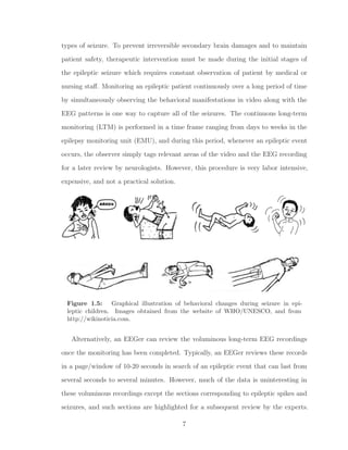
1.5 Graphical illustration of behavioral changes during seizure in epileptic
children. Images obtained from the website of WHO/UNESCO, and
from http://wikinoticia.com. . . . . . . . . . . . . . . . . . . . . . . . 7
1.6 Architecture of a fully automatic patient-specific seizure detection system. 11
3.1 Protocol for analysis of the EEG signals. . . . . . . . . . . . . . . . 39
3.2 Section-based technique of performance evaluation. Numbered events
represent the algorithm detections, EEGer section is a multi-channel
duration event and the ’red’ rectangular box represents the detection
section on channel of interest (LH1-LH3). . . . . . . . . . . . . . . . . 44
xiii](https://image.slidesharecdn.com/039fdf0d-408b-485a-969c-4c8bab29d255-160116041507/85/RY_PhD_Thesis_2012-13-320.jpg)


![Chapter 1
Introduction
Epilepsy is a name given to a collection of neurological disorders. It is usually defined as
a tendency to have recurrent seizures. It is an ancient disorder found in all civilizations,
and it can be traced back as far as medical records exist. In fact, epilepsy is a disorder
that can occur in all mammalian species, probably more frequently as brains become
more complex. Remarkably, epilepsy is also uniformly distributed around the world.
There are no racial, geographical or social class boundaries. It occurs in both genders at
all ages, especially in neonates and in aging population. The clinical features of seizures
are often dramatic and alarming and frequently elicit fear and misunderstanding. This
in turn has led to profound social consequences for sufferers and has greatly added to
the burden of this disease [1].
In this chapter, we introduce some basic concepts in recognition and management
of epilepsy, and motivation for this research. Finally, we will give an outline of the
thesis.
1.1 Epileptic Seizure
Epilepsy is one of the most common and the oldest chronic neurological disorder
known to mankind. It is not a singular disease entity, but a variety of disorders
1](https://image.slidesharecdn.com/039fdf0d-408b-485a-969c-4c8bab29d255-160116041507/85/RY_PhD_Thesis_2012-30-320.jpg)
![reflecting underlying brain dysfunction that may result from many different causes [2].
Approximately, 2% of the world population exhibit symptoms of epilepsy characterized
by the existence of abnormal synchronous discharges in large ensembles of neurons in
the brain structure [3]. This results in one or more clinical symptoms such as loss of
consciousness, behavioral changes, loss of motor activity, loss of senses. At times, it
can lead to death due to unexplained reasons, known as sudden unexplained death
in epilepsy (SUDEP). It is characterized by a tendency to have recurrent seizures. A
person is diagnosed epileptic on the occurrence of two or more unprovoked seizures,
and every year more than 2 million new cases of epilepsy are diagnosed [1, 4-9].
Seizure prevalence increases with age resulting in severe neurological damage that
often becomes medically intractable, a condition in which seizure cannot be controlled
by the administration of two or more anti-epileptic drugs (AEDs). Patients with
medically intractable seizures are often candidates for surgical resection (removal
of the epileptic foci in the brain), which requires accurate localization. Because
of the unknown time of occurrence of seizures, these patients undergo prolonged
monitoring during which a variety of clinical examinations are performed. These
include electrophysiological assessment and neuroimaging evaluation to accurately
identify and localize epileptic foci. Unfortunately, not all patients with intractable
seizure can benefit from resective surgery because of the associated severe systemic
consequences. Alternatively, these patients may benefit by the recent emergence of
novel electroconvulsive and neuromodulation therapies.
1.2 Electroencephalography
Electrophysiological assessment of epileptic patients involves mainly the electroen-
cephalography, which is the primary tool for the clinical recognition and management
of various neurological disorders, including epilepsy. It represents neurophysiologic
2](https://image.slidesharecdn.com/039fdf0d-408b-485a-969c-4c8bab29d255-160116041507/85/RY_PhD_Thesis_2012-31-320.jpg)
![an on-going seizure where the time of occurrence is unknown. That is, continuously
scanning a patient is not possible. Thus, EEG is the only practical approach for
functional long-term continuous monitoring of the brain with a high temporal and
spatial resolution. Recent advances in the new neurostimulating system for epilepsy
rely on the EEG to detect seizures and subsequently abort their progression by
triggering focal treatment (electrical stimulation, focal cooling or drug release) [10-18].
Clearly, EEG plays a significant role from diagnosis to treatment of epileptic patients.
However, interpretation of EEG is notoriously difficult and requires EEG experts
(EEGer) consensus for its recognition.
Figure 1.2: An example of 20 seconds of multi-channel intracerebral EEG of a patient.
1.3 EEG Classification
The EEG consists of signals from both the cerebral and non-cerebral origins. Depending
on the recording technique, the contribution from each may vary. Abnormal EEG
patterns are specific to the type of study being performed. It is the task of the EEGer
to recognize the waveform of interest from the observed EEG and to identify the likely
locations of their generators. Since intracerebral or subdural electrodes are usually
4](https://image.slidesharecdn.com/039fdf0d-408b-485a-969c-4c8bab29d255-160116041507/85/RY_PhD_Thesis_2012-33-320.jpg)
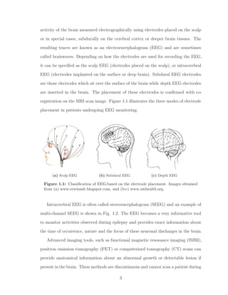
![closer to neurons than the scalp electrodes, the amplitude of EEGs recorded by the
depth electrodes is usually larger than that from scalp electrodes [19-21]. When EEG
is recorded with scalp electrodes, the amplitude is of the order of 20µV to 100 µV , and
of the order of 100 µV to 2 mV when recorded using depth electrodes. The spectral
bandwidth of the EEG (normal and abnormal) is from under 0.5 Hz to about 500 Hz.
The EEG experts visually inspect the prolonged recordings to identify epileptiform
activities. The common approach utilized to classify EEG is shown in Fig. 1.3.
Interictal EEG is defined as the non-seizure activity or the background EEG. The
interictal EEG comprises of normal patterns as well as abnormal patterns (such as
spikes, high frequency oscillations, etc) along with normal rhythmic discharges such
as alpha rhythm and sleep spindles [5, 22-27].
Generally, most of the seizures have some common characteristics, such as rhythmic
discharge of large amplitude or a low amplitude desynchronized EEG at the onset,
and repetitive spikes and irregular slow waves. No two patients have identical ictal
pattern. Even within the same patient, the two ictal patterns are never identical
though similar. Thus, the definition of a seizure still remains vague. However, the most
widely accepted definition for seizure states that during an epileptic seizure, a new
type of EEG rhythm appears, hesitantly, and then more distinctly, and soon it boldly
dominates the EEG tracing. It tends to become slower with increasing amplitude and
the more distinct spiky phases of the rhythmical waves observed in an EEG recording
[5]. An example of such a seizure is shown in Fig. 1.4.
5](https://image.slidesharecdn.com/039fdf0d-408b-485a-969c-4c8bab29d255-160116041507/85/RY_PhD_Thesis_2012-34-320.jpg)
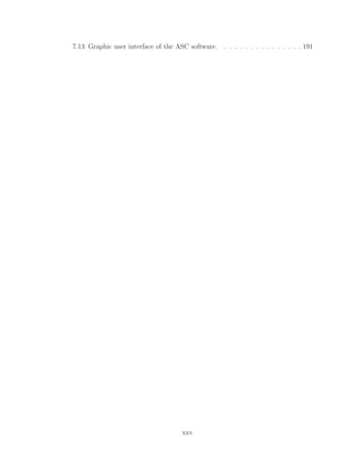
![EEG
Normal
Abnormal
Epileptiform
Non-epileptiform
Spikes
Seizure
Figure 1.3: Schematic for classification of EEG in epilepsy by the EEGer. Adapted
from Self-adapting algorithms for seizure detection during EEG monitoring by H. Qu,
1995, McGill University, Canada [20].
Figure 1.4: An example 20 seconds of SEEG representing ictal (seizure) and interictal
activity for a patient
Early stages of an epileptic seizure provide information about the seizure focus,
type and various characteristics of clinical significance. Seizures can be divided into
two distinct categories: (a) clinical and (b) sub-clinical. Clinical seizures are recognized
by certain behavioral changes associated with the seizure. Behavioral symptoms in
epileptic children are illustrated in Fig. 1.5. In some patients, there is minimal
or no behavioral changes during an epileptic seizure. Such seizures are known as
electrographic or sub-clinical seizures. EEG captures the abnormal activity in both
6](https://image.slidesharecdn.com/039fdf0d-408b-485a-969c-4c8bab29d255-160116041507/85/RY_PhD_Thesis_2012-35-320.jpg)

![methods often fail to detect seizures occurring on a few channels, i.e., focal seizures that
occur on spatially separated channels. To improve sensitivity and specificity, a handful
of patient-specific seizure detection methods, that are based on the recurring nature
of epileptic seizures, have been proposed. Isolating precisely reproducible phenomena
in EEG signals still remains a difficult task that can highlight the neurophysiological
mechanisms to characterize an epileptic brain. Patient-specific seizure detection
systems thus become an indispensable tool aimed at better defining and understanding
epileptogenic areas to improve surgical treatments [28, 29].
Even though patient-specific seizure detectors demonstrate improved performance
over the generic methods, they are not practical. The main limiting factors in
all patient-specific detectors are (a) supervised selection of the seizure EEG, (b)
supervised selection of the non-seizure EEG (or a set of non-seizure EEG patterns),
and (c) supervised training of the classifier. Another fundamental problem in all seizure
detection methods is the detection of seizures with subtle changes in the amplitude [30-
37]. This is a problem that persists even in the visual detection of seizures. Addressing
some of these limitations will lead to a more practical patient-specific detector.
In addition to the seizure detection, one of the primary aims of the review of
prolonged intracranial EEG monitoring is to map channel-by-channel timeline of
seizures and epileptiform activities that can provide visualization of seizure onset
and spread (both temporally and spatially), which is pivotal when planning resective
surgery. This type of 2D visualization is unavailable for the review of intracranial
EEG. Automatic seizure detection can aid in the rapid identification of seizures.
However, it does not allow for a quantitative seizure analysis, which is still done
manually by experts. Therefore, adjunctive methods that allow quick identification of
seizures, provide a view of seizure activity over prolonged durations, seizure recurrence
frequency, and sites involved in the seizure generation for therapeutic interventions,
and management are much needed in the EMUs [5, 38-42].
9](https://image.slidesharecdn.com/039fdf0d-408b-485a-969c-4c8bab29d255-160116041507/85/RY_PhD_Thesis_2012-38-320.jpg)
![Prolonged intracranial EEG recording is also performed prior to the implantation
of a neurostimulating device to identify the seizure foci and neural areas for stimulation
therapy for patients who may not benefit from the resective surgery. The idea behind
neurostimulation devices is to deliver focal treatment to inhibit the epileptic activity.
Electrical stimulation of the epileptogenic foci to inhibit the progression of seizure
is one such method that is gaining popularity [13-16, 18, 43, 44]. The success of
such devices rely heavily on the seizure detection capabilities. Computationally light,
low-power, robust and patient-specific seizure detectors are prerequisite to maintain
the longevity of the device (battery) and patient safety. However, seizure detection
system for application in the neurostimulating device is still in its infancy.
A fully automatic patient-adaptive seizure detection system is much needed, but
the clinical requirements of the seizure detection system and the existing challenges
in the non-patient specific (NPS) and patient-specific (PS) approaches of seizure
detection do not allow the existence of such a system. However, a fully automated
patient-adaptive seizure detection system is feasible by combining NPS and PS systems
to capture the advantages of the two approaches. The architecture of such a system is
shown in Fig. 1.6. Automatic patient-adaptation in such a system may be possible
by addressing the limitations in the PS systems, that is, by removing the need for a
large background EEG, automating the selection of the template seizure pattern and
training of the classifier. In such a system, the NPS system bootstraps the PS system
with template seizure patterns, and the PS system leverages on the event it detects to
optimize itself. It may be possible that seizures that are difficult to be detected by
the NPS system are easily identifiable by the PS system. Conversely, seizure patterns
that are difficult to be detected by the PS system are detected by the NPS system.
The patient-specific pattern database is updated on subsequent detections. Then,
the patterns in the database, ranked based on their recurrence frequency via the PS
system, may allow the experts to perform rapid qualitative and quantitative analysis.
10](https://image.slidesharecdn.com/039fdf0d-408b-485a-969c-4c8bab29d255-160116041507/85/RY_PhD_Thesis_2012-39-320.jpg)
![Thus, the time involved in the manual qualitative analysis of the detected patterns,
quantification of reproducible seizure patterns, and correlation with the clinical data,
reduces significantly. However, realization of such a system demands that both the
NPS and PS systems are computationally light and robust.
Figure 1.6: Architecture of a fully automatic patient-specific seizure detection system.
In this thesis, we aim to develop new NPS and PS systems that can be used in the
fully automatic PS seizure detection system of Fig. 1.6.
Spike Classification
In addition to seizures, epileptic spikes also play an important role in the diagnosis
of seizure onset zones. They tend to occur more frequently than seizures and are
linked to the seizure onset zones. Detection and classification of spikes thus can
improve the epilepsy management. Furthermore, several studies have reported a
better surgical outcome when regions of frequent spikes (interictal) are also removed
[45]. However, it is still unclear as to exactly how interictal spikes develop, and how
they propagate and contribute to the generation of seizures [46-48]. A recent study
examined human brain tissues at regions of seizure onset and found a small group
of genes highly correlated with the interictal spike frequency [49, 50]. Quantitative
analysis of interictal spiking thus becomes inevitable, and may help to identify epileptic
biomarkers for drug therapy.
11](https://image.slidesharecdn.com/039fdf0d-408b-485a-969c-4c8bab29d255-160116041507/85/RY_PhD_Thesis_2012-40-320.jpg)
![1.6 Organization of the Thesis
The thesis is organized as follows.
Chapter 2 reviews popular seizure detection and spike sorting methods.
Chapter 3 describes the EEG data used to develop and evaluate the performance
of the methods proposed in this thesis.
Chapter 4 describes three new, computationally simple, data driven NPS systems.
The NPS systems quantify the continual increase (temporal evolution) in the seizure-
related EEG characteristics to make detections. This chapter presents results obtained
on the training dataset.
Chapter 5 presents performance evaluation results on the test data for the new NPS
methods compared against three popular comparison systems (Gotman system [51],
Reveal algorithm [52], and Grewal-Gotman system [32]). This chapter also describes a
new digital trending tool aimed to facilitate rapid review of prolonged EEG recordings
in the EMU.
Chapter 6 describes a new model-based PS system suitable for the development
of a fully automatic PS system. The PS system is developed in the framework of
statistically optimal null filters, which is a novel approach for solving the problem
of enhancement/suppression of narrowband signals of short-record length. The per-
formance of the new model-based PS system is compared with that of the popular PS
system of Qu-Gotman [21]).
Chapter 7 describes a new graphical user interface (GUI) software package for
automatic classification of epileptic spikes in the intracranial EEG recordings. The
chapter describes the data utilized in the development, validation strategy and the
spike classification algorithm. An easy-to-use GUI is developed that facilitates easy
integration of the method in the clinical settings.
Finally, in Chapter 8, concluding remarks highlighting the contributions of the
thesis and suggestions for further investigation are provided.
13](https://image.slidesharecdn.com/039fdf0d-408b-485a-969c-4c8bab29d255-160116041507/85/RY_PhD_Thesis_2012-42-320.jpg)
![Chapter 2
Literature Review
2.1 Introduction
This chapter provides an overview of published research on seizure detection and spike
sorting. A plethora of seizure detection and spike sorting algorithms1
exists in the
literature. We limit our discussion to some of the recent and landmark approaches of
seizure detection and spike sorting methods, with particular attention to the algorithms
that are relevant to this research work.
2.2 Automatic Seizure Detection
The topic of seizure detection has gained much attention in recent years due to its
evidence in prognosis, diagnosis and as a therapeutic tool in the epilepsy care along
with the availability of low-cost, fast computation tools. Chapter 1 introduced the
role of EEG in epilepsy care and management and discussed some of the existing
challenges in the design of the automatic seizure detection (ASD) systems. The study
of Ives and Woods [53] on 100 patients reported 30% of seizures as only electrographic
1
It is important to note that the spike sorting algorithms reviewed in this chapter are designed
specifically for the action potentials that are also called spikes and not for the epileptic spikes.
Nonetheless, the process in these methods can be employed for epileptic spike classification.
14](https://image.slidesharecdn.com/039fdf0d-408b-485a-969c-4c8bab29d255-160116041507/85/RY_PhD_Thesis_2012-43-320.jpg)
![changes with no observable behavioral manifestations. This study demonstrated the
importance of EEG monitoring and the role of ASD systems without which it would
have been virtually impossible to detect purely electrographic seizures. Majority
of ASD systems are designed to facilitate the review of prolonged EEG recordings,
whereas only a few ASD systems are designed to perform online detection during
the monitoring session. Care and management of an epileptic patient are dependent
on the ASD system. Therefore, automatic seizure detectors must have a very high
sensitivity (proportion of seizures that are detected) and a very low false detection
rate (FDR). In the EMU settings, the detection sensitivity is of more importance
than the FDR, since missed seizures may never be reviewed by the EEGer, and are
therefore of more serious consequence [22, 54]. Both sensitivity and FDR are equally
important in neurological intensive care unit (NICU) applications, as large number
of false detections are annoying and require additional staff vigilance in a very busy
and stressful environment [55-59]. In certain applications of ASD systems, the time
lag associated in a seizure detection is also important. For example, neuroresponsive
therapy (NRT) application requires the ASD system to predict/detect seizure as early
as possible to initiate preventive measures.
The first automatic seizure detection method designed to detect seizures with
sustained paroxysmal rhythmic activity is the pioneering work of Gotman [51, 54] and
is an industry standard in seizure detection. Since then, there has been a marked
increase in seizure-related research. ASD systems are available (a) as seizure onset
detectors, (b) as seizure pattern detectors or (c) as seizure prediction systems. A
seizure onset detector aims to detect seizures at the onset, which inherently results
in a higher rate of false detection. Some methods aim to detect the seizure patterns,
improving FDR rate at the cost of increased detection delay, while a few methods
predict seizures minutes or even hours in advance. However, such systems report none
to minimal success in predicting seizures.
15](https://image.slidesharecdn.com/039fdf0d-408b-485a-969c-4c8bab29d255-160116041507/85/RY_PhD_Thesis_2012-44-320.jpg)
![prior to usage. Table 2.1 provides a summary of the ASD systems according to the
categories described above.
Clearly, the challenges facing the designer of an automatic seizure detector are
significant. No one detector can easily satisfy the varying requirements, and is the
reason for the existence of many seizure detection methods in the literature. In this
thesis, we broadly categorize automatic seizure detection into two groups:
• NPS seizure detection
• PS seizure detection
2.2.1 Non-Patient-Specific Seizure Detection
Gotman [54] designed a seizure detection system, which detected seizures based on
decomposing EEG signals into half-wave components and analyzing them in 2-second
epochs. The features selected to characterize seizures were the zero-crossings, half-
wave amplitude, and rhythmicity. Relative to a background that trails the test
epoch, a seizure detection occurs in the test epoch when the features exceed the pre-
defined detection thresholds. Detections in individual channels are combined in some
spatio-temporal context for final detection. Numerous types of seizures were detected
by this method in 22 scalp EEG recordings (mean duration 12.4 h) and 44 depth
EEG recordings (mean duration 18.7 h). The method was subsequently improved
by increasing the distance between the background and test epoch to account for
seizures with a gradual onset [51]. By altering the amplitude parameters, the method
was capable of detecting low amplitude seizure discharges. Additionally, enhanced
temporal context further reduced the false detections caused by short rhythmic bursts.
A patient alarm was introduced to automatically record ictal event when either the
patient or nurse became aware of a seizure onset. These modifications on 293 h of
EEG of 49 patients resulted in an overall sensitivity ranging between 70-80% with a
17](https://image.slidesharecdn.com/039fdf0d-408b-485a-969c-4c8bab29d255-160116041507/85/RY_PhD_Thesis_2012-46-320.jpg)

![FDR of 0.84/h in scalp EEG and a FDR of 1.35/h in depth EEG [51]. Many of the
concepts introduced by Gotman continue to be pervasive in seizure detection research.
Pauri et al. [96] evaluated the method of [51] in a clinical setting. The EEG
data of twelve patients with medically intractable partial seizure, who had undergone
video-EEG monitoring over 1-15 days (mean 10.5 days), were marked with the help
of the Gotman ASD system and fast video review. Detections in individual channels
were rated from 1 to 4 according to their likelihood of being genuine. The method was
tested with several settings. A total of 461 hours of EEG having 216 seizures from
twelve patients were analyzed. The two best performing settings showed a sensitivity
of 81.4% with a FDR of 5.38/h and a sensitivity of 73.1% with a FDR of 5.01/h. The
study demonstrated the need for tunable detection thresholds in ASD systems.
Harding [97] proposed a system to detect seizures (temporal lobe epilepsy) by
detecting spiking phases using two main features: (1) magnitude of the sample-to-
sample difference, and (2) the time difference between large magnitude spikes to
determine the spiking rate. In this method, the number of large magnitude spikes are
counted in a 5 s epoch and when the counter value exceeds a pre-defined threshold, a
detection is made. The magnitude of a spike is considered large if it is greater than
the running average of the background spikes scaled by a signal-to-background ratio
(SBR). Spiking rate and rhythmicity are used to differentiate between the seizure
activity and the spike bursts or artifacts. The method was tested on 40 patient EEG
data with a total of 416 seizures over 1578 hours, and resulted in a sensitivity of 92.6%
and a FDR of 1.94/h. The detection threshold was adjusted for individual patients on
observation of the first seizure.
Gabor et al. [98] proposed a self-organizing map (SOM) neural network-based
seizure detector named as CNet. In this method, the individual channels are filtered
using a wavelet transform-based matched filter followed by 256-point FFT. Input to
the SOM were the 256 coefficients that constituted the feature vector. The method
19](https://image.slidesharecdn.com/039fdf0d-408b-485a-969c-4c8bab29d255-160116041507/85/RY_PhD_Thesis_2012-48-320.jpg)
![detected seizures with a sensitivity of 90% and a FDR of 0.79/h. The weak aspects in
this study are the use of a high-dimensional feature vector, pre-selection of the seizure
type (frontal and temporal lobe) and tuning of the detection parameters to optimize
the performance. In a subsequent study [99], the authors validated the performance
of their method against two commercial seizure detection algorithms, namely, Monitor
(Stellate Systems Inc.) and audio-transformation (Oxford Medilog). The methods were
evaluated on 4553.8 h of EEG data of 65 patients. CNet resulted in a sensitivity of
92.8% with a FDR of 1.35/h, Monitor resulted in a sensitivity of 74.4% sensitivity with
a FDR of 3.02/h, and audio-transformation method reported a sensitivity of 98.3%
(false detection was not reported because of the subjective nature of the method). The
authors demonstrated variation in the performance of the algorithm on data previously
unseen by the algorithm.
Osorio et al. [100] proposed a real-time seizure detection system with short
detection delay. The EEG is filtered in the frequency range of 5-40 Hz using a wavelet
finite impulse response (FIR) filter. The filtered EEG is squared, median filtered and
compared to a background signal. The method was tested on 125 seizures reporting
100% sensitivity and zero false positives. The authors claim the method to be generic,
but on close inspection, it seems to be specific to a group of patients (mesial temporal
seizures). Furthermore, the method has neither been validated on continuous data nor
on previously unseen data, thus contributing to overestimated performance.
Khan and Gotman [101] proposed a seizure onset method to improve the per-
formance of [51] for depth EEG recordings. The method requires a minimum of two
channels for detection and employs wavelet decomposition to separate the EEG into
frequency scales. A number of features are calculated for each scale and applied
to empirical decision thresholds. The method was evaluated on 229 hours of depth
EEG from 11 patients that resulted in a sensitivity of 85.6% with a FDR of 0.3/h.
Note that the wavelet decomposition into different scales hinders the clinical use of
20](https://image.slidesharecdn.com/039fdf0d-408b-485a-969c-4c8bab29d255-160116041507/85/RY_PhD_Thesis_2012-49-320.jpg)
![the method, since different clinical settings record EEG at different sampling rates.
This research was extended in [102] for scalp EEG and in [32] for depth EEG. The
limitation introduced by wavelet decomposition is addressed by the use of filter-banks
and the limitations of the empirical thresholds with an approximate Bayesian classifier.
The method included a user tunable threshold, which allows for trade-off between
sensitivity, detection delay, and FDR. The data is processed in 4 s epoch and is filtered
by a filter-bank similar to wavelet decomposition. Relative energy, relative amplitude,
and coefficient of variance of the amplitude were adapted from the previous work of
[101]. Once the EEG data is separated into frequency bands, each frequency band has
a combination of five features to create a feature vector. Using Bayes theorem, the
classifier is trained to separate the two classes. The method was evaluated on 360 h of
EEG and resulted in a sensitivity of 77.9% with a FDR of 0.85/h for scalp EEG and a
sensitivity of 86.4% with a FDR of 0.47/h for depth EEG without any tuning.
Iasemidis et al. [103] proposed a short-term maximum Lyapunov exponent
(STLmax)-based seizure prediction and detection system to assist in easy review
of EEG recordings. The authors in subsequent studies [68-73] demonstrated a pro-
gressive dynamical entrainment of electrode sites as seizure onset approaches. The
method has been validated on single as well as on the multi-channel EEG recording
from 2-5 patients that resulted in prediction sensitivity ranging between 82-91% and
FDR between 0.16-0.19/h. The method has not been validated on a large data set
and is designed for a specific type of seizure (TLE). However, the method is promising
for therapeutic application.
Wilson et al. [52] proposed the Reveal algorithm based on Matching Pursuit (MP),
small neural-network-rules and connected-object hierarchical clustering based seizure
detection system for clinical application in the EMU. The EEG is decomposed into a
set of ’atoms’ each localized in time and frequency using the MP algorithm. From
the resulting set of atoms, temporal features are extracted relative to a background
21](https://image.slidesharecdn.com/039fdf0d-408b-485a-969c-4c8bab29d255-160116041507/85/RY_PhD_Thesis_2012-50-320.jpg)
![and combined with spatial information to develop a set of rules, which authors have
referred to as neural network-rules. The detections are clustered together towards the
final detection. The algorithm has been validated on a large dataset and compared
with two other methods CNet and Sensa (Stellate Systems). The method included 676
seizures from 1046 hours of EEG recording and resulted in a sensitivity of 76% with a
FDR of 0.11/h, whereas CNet and Sensa reported sensitivities of 48.2 and 38.5% with
FDR of 0.75 and 0.11/h respectively. The method is another widely accepted clinical
seizure detection tool used in the EMU.
Navakatikyan et al. [110] proposed a waveform-based (morphology) neonatal
seizure detection algorithm to detect heightened regularity in EEG wave sequences
using wave intervals, amplitudes and shapes. The algorithm involves several steps
mimicking human experts. It includes filtering the EEG signal, parallel fragmentation
of EEG signal into waves, wave-feature extraction and averaging, and elementary,
preliminary and final detection. The EEG trace is fragmented into waves using a
moving average technique to determine the points of intersection with the EEG signal.
Then, each wave is partitioned into two halves based on the local maxima and minima
of the wave. The positive half of the wave is defined as peak-wave and negative
half of the wave as the trough wave. To quantify increased regularity in the EEG
waveforms during seizure, the peak- and trough- waves are matched with the peak-
and trough- waves of previous two consecutive waves. The average of the previous
four matching parameters (correlation coefficient) is compared to a threshold to detect
seizure. The performance of the algorithm was assessed against Gotman [111] and Liu
[112] algorithms and resulted in sensitivity ranging between 83-95% when tested on 55
neonate EEG data. The method of Gotman [111] and Liu [112] resulted in sensitivities
ranging between 45-88% and 96-99% respectively. This study (along with the study of
[51, 97, 113]) suggests that methods based on morphological features tend to perform
better over the ASD techniques that employ the more popular segment-based features
22](https://image.slidesharecdn.com/039fdf0d-408b-485a-969c-4c8bab29d255-160116041507/85/RY_PhD_Thesis_2012-51-320.jpg)
![for classification.
Aarabi et al. [114] proposed an adaptive neuro-fuzzy inference-based seizure
detection system for depth EEG recordings. In this method, the measures employed
to quantify seizure were adapted from [32] and [115]. The measures are input to a rule-
based classifier which detects seizure on individual channels. The individual channel
detections are combined in some spatio-temporal context to make a multichannel final
detection. The study reported a sensitivity of 98.7% and a FDR of 0.27/h for depth
EEG from 21 patients. The study considered only clinical seizures with an average
duration of 102 s and excluded all subclinical and short seizures from their analysis.
Kelly et al. [116] proposed the IdentEvent seizure detection method for scalp
EEG that has recently received FDA approval for clinical use in review of EEG
recordings. The method employs three descriptors: pattern-match regularity statistic,
local maximum frequency, and amplitude variation, in order to identify seizures. The
IdentEvent algorithm performance has been evaluated on 1208.24 hours of the scalp
EEG of 55 patients that resulted in positive percentage agreement value (PPV) of
79.5% and a FDR of 2/h and is compared against the Reveal algorithm [52]. Reveal
algorithm was evaluated at three different detection settings that resulted in PPV
ranging between of 74-80% with FDR ranging between 6-13/h.
Duun-Henriksen et al. [117] have investigated the performance of automatic seizure
detection using only a few recording channels. The method operates in two stages:
first, it selects the channels used for analysis based on a simple feature, and then it
performs seizure detection using a support vector machine-based classifier with wavelet
domain features. Data from 10 patients undergoing presurgical invasive monitoring
with 48-64 channels sampled at 239.75 Hz were considered to train and test the ASD
system. The data contains a total of 59 clinical seizure in 1419 h of recordings. The
study reports minimal improvement in the sensitivity by the algorithm over the EEGer
on a set of preselected channels having highest variance and entropy between the two
23](https://image.slidesharecdn.com/039fdf0d-408b-485a-969c-4c8bab29d255-160116041507/85/RY_PhD_Thesis_2012-52-320.jpg)
![groups. Note that the selected channel may not always remain the highest variance
channel at all times during the monitoring session. Furthermore, the study did not
include sub-clinical and focal seizures in the performance evaluation. Therefore, the
claims may not hold true for all types of epileptic seizures.
Recently, Majumdar and Vardhan [118] have proposed a differential operator and
windowed variance based seizure detection system that yielded 91.5% sensitivity and
a FDR of 0.12/h on 15 patients depth EEG recording. It is interesting to note that
the method quantifies abnormally sharp activities to make a seizure detection similar
to our work in [33, 34, 119, 120], but using different features. Authors excluded six
patients on which their method did not perform satisfactorily. Furthermore, this
method did not detect subclinical seizures in this data.
2.2.2 Patient-Specific Seizure Detection
Qu and Gotman [21] introduced the concept of patient-specific seizure detection using
a template matching approach. During LTM, once a seizure occurs in a patient, its
onset is manually selected and stored. A large background preceding the seizure is also
selected. This information about the seizure and the background is utilized to train a
classifier. During subsequent monitoring sessions for the given patient, the EEG is
scanned for a good match to the template seizure using the trained classifier; when one
is found, it is reported immediately as the onset of a similar seizure. The classifier used
in the method is a modified nearest-neighbor classifier. The method is not automatic
and its applicability in clinical setting is limited because of the requirement of manual
selection of the template seizure pattern and manual selection of a large background
EEG. Additionally, the training of the classifier is complex. However, this study
opened new avenues towards building new PS seizure detection schemes.
Wendling et al. [28] proposed a method to quantify similar seizures using a modified
Wagner and Fischer’s algorithm . The process involves (i) segmentation of depth EEG
24](https://image.slidesharecdn.com/039fdf0d-408b-485a-969c-4c8bab29d255-160116041507/85/RY_PhD_Thesis_2012-53-320.jpg)
![signals, (ii) characterization and labeling of the EEG segments, and (iii) comparison
of observations coded as sequences of symbol vectors. The third step is based on a
vectorial extension of the Wagner and Fischer’s algorithm [121] to first quantify the
similarities between observations and then to extract invariant information, referred to
as spatio-temporal signatures. The study reported reproducible mechanisms occurring
during seizures for a given patient. In subsequent studies on medically refractory
partial seizures, the authors demonstrated reproducible propagation schemes that may
help in the understanding of epileptogenic networks [122, 123].
Shoeb et al. [124] proposed a multichannel seizure onset detector system using
wavelet decomposition to capture morphological and spatial information that con-
stituted feature vector as an input to a support vector machine (SVM) classifier
for the presence of seizure. The method requires prior knowledge of at least 2-4
seizures, and non-seizure background EEG. The trained classifier is used to detect
subsequent seizures in the record. The method was evaluated on 36 pediatric scalp
EEGs resulting in a sensitivity of 94% with a FDR of 0.25/h. In contrast to other
PS methods, where only a single seizure pattern is used for training, this method
requires more than one template seizure pattern. The method has been considered in
a neuroresponsive therapy [125], where the EEG features were computed within the
implantable device.The features were then transmitted to a high performance remote
computer for classification. Authors suggest that remote classification reduces the
computational cost and is aimed at extending the implant’s battery life. However, a
centralized remote system for seizure classification is not a practical solution.
Osario et al. [64, 90-93] extended their originally proposed NPS method [100] in
the design of PS system to prevent propagation of a seizure using electrical stimulation.
A set of candidate filter banks based on the power in the different spectral bands
are designed using a priori known seizure and non-seizure patterns. The filter that
maximally separates the seizure and non-seizure is selected to train the classifier. The
25](https://image.slidesharecdn.com/039fdf0d-408b-485a-969c-4c8bab29d255-160116041507/85/RY_PhD_Thesis_2012-54-320.jpg)
![trained classifier is used to detect remaining seizures in the data. The authors selected
short segments of seizure and non-seizure to demonstrate their method. However, the
scheme has not been validated on prolonged and continuous EEG recordings.
Wilson et al. [130, 131] presented a neural network architecture to design a
PS method (known as MagicMarker) similar to their Reveal algorithm. It trains
the PS classifier rapidly without human intervention, requires minimal sample data,
and employs a supervised learning algorithm to improve classification errors. The
probabilistic neural network (PNN) is trained on a single seizure event and the
corresponding background activity that extends from the end of the previous seizure
event (or the beginning of the record) to the start of the current seizure event. Although
the method requires a single seizure pattern, it needs extensively long background
EEG, thus limiting its practical application.
Shi et al. [132] proposed a model-based seizure detection using statistically optimal
null filter (SONF) which requires only the a priori knowledge of a single seizure
pattern. The authors proposed sinusoidal wavelet basis function to model the template
seizure. The approach provided 100% sensitivity and no false detection on single
channel study of two patients. However, the method has several drawbacks: (1)
it is not automatic, (2) involves visual segmentation of the template pattern, (3)
employs wavelet domain-based modeling of the template pattern, and (4) has not been
validated on large dataset. Addressing the limitation to this method may lead to the
development of an automatic, robust and more practical PS system.
Zandi et al. [35] proposed a patient-specific seizure detection method for scalp
EEG recording based on wavelet packet transform. The method requires a priori
knowledge of the seizure and a large background EEG (∼30 min.). The seizure and
background EEG is analyzed in a 2 s moving window with 50% overlap. Each epoch
is decomposed into a wavelet-packet tree. Energy in each sub-band is used to estimate
the probability density function of each sub band relative to a reference, to estimate
26](https://image.slidesharecdn.com/039fdf0d-408b-485a-969c-4c8bab29d255-160116041507/85/RY_PhD_Thesis_2012-55-320.jpg)
![the distance between seizure and non-seizure. In addition, regularity index is also
computed from the decomposed wavelet packets to train the classifier. The combined
seizure index which measures increased regularity and energy index on the individual
channels are combined with multichannel information to identify seizures similar to
the template seizure. The method has been validated on 14 patients resulting in a
sensitivity of 90.5% with a false detection rate of 0.51/h. The PS scheme has several
drawbacks: not automatic, selection of very large non-seizure reference, wavelet-packet
based analysis, manual tuning of the detection thresholds, and selection of specific
type of seizure dataset (temporal lobe epilepsy).
Salam et al. [133] recently proposed a low-power patient-specific seizure onset
detector for implantable devices. The method is based on the concept of detecting
progressive increase in the amplitude and frequency at the seizure onset to make
accurate seizure detection proposed in [33, 34, 36, 98-100]. Based on this concept, the
authors devised an algorithm that consists of a set of voltage and frequency detectors
to identify a progressive increase in the amplitude and frequency at the seizure onset in
multiple frequency bands. The detection thresholds are customized for each individual
patient to maximize specificity and to prevent unwarranted neural stimulation. The
algorithm is validated on seven medically refractory epileptic patients with a report
of 100% specificity and average onset delay of 13.5 seconds. The method is designed
specifically for seizure that progressively increases with low-voltage fast-activity. Note
that specificity can be maximized to 100%, but at the cost of sensitivity, which has
not been reported in this study. Further, the method has also not been validated on
varied and large intracranial EEG recordings.
27](https://image.slidesharecdn.com/039fdf0d-408b-485a-969c-4c8bab29d255-160116041507/85/RY_PhD_Thesis_2012-56-320.jpg)
![2.3 Spike Sorting Techniques
Patients with medically refractory seizures are candidates for surgical resection of the
seizure onset area or for deep brain stimulation therapies that can lead to significant
reduction or cessation of seizures. Several studies report a better surgical outcome when
regions of frequent interictal spikes are also removed [45, 101-106]. However, as to how
exactly the interictal spikes develop and as to how they propagate and contribute to
the generation of seizures is not well understood [107-109]. Automatic spike detection
techniques have received intense attention to aid rapid identification of spikes in the
voluminous EEG recordings. However, quantitative analysis of epileptiform spikes is
still done manually which is a very labor-intensive and time consuming task.
On the other hand, spike2
classification is the first step in experimental neuro-
physiological studies aimed to better understand the brain functions. Classification of
spikes is studied since (1) spikes are highly stereotypical, permitting the modeling of
their shapes to facilitate classification of the associated neurons, (2) spike trains carry
an affluent amount of information permitting modeling of brain functions at very high
temporal and spatial resolutions, and (3) spike occurrences mediate plasticity such
as learning and memory formations [110-112]. However, spike classification schemes
mainly focus on the timing of their individual occurrences (spike train analysis) and
not on their actual shapes [146, 147]. A relatively large number of spike classification
methods have been proposed for neuro-physiological experiments. The following
presents some of the popular spike classification methods.
Willming and Wheeler [149] proposed a four channel extracellular spike sorting
algorithm based on spike amplitude. The classification routine considered a spike to
belong to the same class when the peak amplitude fell within a user specified interval.
2
It must be noted that spikes in the EEG and in the basic neurophysiological experiments are
two different entities. The use of the term ’spike’ in experimental neurophysiological studies refer
to action potentials, recorded using microelectrodes (1 ms events) that represent the normal and
abnormal functions of single/multi-cell neurons. The epileptic spikes in the EEG are recorded with
macroelectrodes that typically last 35 to 200 milliseconds.
28](https://image.slidesharecdn.com/039fdf0d-408b-485a-969c-4c8bab29d255-160116041507/85/RY_PhD_Thesis_2012-57-320.jpg)
![The authors proposed two more approaches that compared the RMS error between the
stored templates of each unit’s spike waveform and the spike most recently detected.
The new spike was classified according to the minimum of the RMS errors computed.
The third algorithm utilized principal component analysis (PCA) for classification.
Peak amplitude windowing-based algorithm outperformed the principal component
and template matching algorithm. The signal-to-noise ratio of the spikes and large
variation in the spike waveforms justifies the poor classification by template matching
approach compared to peak-amplitude and principal component approaches.
Chandra and Optican [150] proposed a connectionist neural network for sorting
extracellular spike recordings. Spikes were detected when the amplitude of the recorded
signal exceeded a positive or negative threshold. Detected spikes were clustered together
to form noise-free templates using the simultaneous clustering algorithm, which first
finds the best clusters around each waveform, groups these initial clusters together
and then selects the best and final clusters. Each detected waveform is initially a
potential initiator waveform for a cluster. The waveforms are clustered with the
initiator waveform based on the best alignment and Euclidean distance, resulting in
M clusters for M waveforms. The clusters are selected based on inter-cluster distance,
cluster density and a cluster-scatter measure. Centroids of the selected clusters are
the templates. A fully connected feed-forward, three layer trained neural network
examines the template and spikes. The performance was determined on simulated
data.
Quiroga et al. [151] proposed a method for detecting and sorting spikes from
multi-unit extracellular recordings. The method combines wavelet transform and
super-paramagnetic clustering and encompasses three principal stages. Spikes are
detected with an automatic amplitude threshold on the high-pass filtered data and a
small set of wavelet coefficients from each spike is chosen as input for the clustering
algorithm. Clustering algorithm is based on simulated interaction between each
29](https://image.slidesharecdn.com/039fdf0d-408b-485a-969c-4c8bab29d255-160116041507/85/RY_PhD_Thesis_2012-58-320.jpg)
![data point and its k-nearest neighbors, which is implemented as a Monte Carlo
iteration of a Potts model. The complete clustering algorithm is known as super-
paramagnetic clustering algorithm. The algorithm outperformed when compared to
other conventional methods using several simulated data sets whose characteristics
closely resemble those of in vivo recordings. The unsupervised and fast implementation
of the sorting technique is commonly known as WAVE CLUS.
Wood et al. [152] studied variability in manual spike sorting and its implications in
the neural prosthetics. The study highlighted the challenges encountered in manually
sorting a large number of multi-channel data and the need for a robust spike sorting
algorithm.
Kaneko et al. [153] proposed tracking spike-amplitude changes to improve the
sorting results. Their sorting algorithm included spike detection, spike vectorization,
burst detection, and spike classification. A spike was detected by matching the
recorded waveforms with a set of spike templates with different durations (spike
detection). The amplitudes of these waveforms constituted a spike-amplitude vector
(spike vectorization). Spike bursts were detected based on attenuation of the spike
amplitude and inter-spike intervals (ISIs) (burst detection). Finally, clusters of spike-
amplitude vectors in the six-dimensional vector space were statistically classified by
bottom-up hierarchical clustering in which every spike-amplitude vector was first
assigned to a cluster, and then the nearest clusters were repeatedly combined into a
new cluster until clustering ended by Mahalanobis generalized distance. The study
reports that cluster tracking improves the quality of multi-neuronal data analysis
resulting in compact clusters.
Wolf et al. [154] proposed an unsupervised algorithm for sorting and tracking
action potentials of individual neurons in multi-unit extracellular recordings. This
approach assumes that each neuron produces spikes whose waveform features vary
according to a probability distribution, and thus, each generating neuron may be
30](https://image.slidesharecdn.com/039fdf0d-408b-485a-969c-4c8bab29d255-160116041507/85/RY_PhD_Thesis_2012-59-320.jpg)
![represented as a component in a mixture model. Additionally, the method incorporates
the knowledge of available information over time to re-identify previously identified
neurons despite possible changes in the amplitude, phase, and numbers of neuronal
signals. This is achieved by dividing the long recordings into short time intervals
followed by temporal alignment of spike events. The detected spike waveform is then
projected onto a d-dimensional feature space, and are clustered by optimizing the
Gaussian mixture models (GMM) via expectation–maximization (EM). Validation
of the sorting algorithm on the recordings from macaque parietal cortex showed
significantly more consistent clustering and tracking results than traditional methods
based on EM optimization of the mixture models.
Chan et al. [155] proposed an unsupervised spike sorting method for extracellular
recordings. It is based on wavelet coefficients, spike alignment and template-matching.
The method uses significant wavelet coefficients near the alignment point to improve
the sorting results. Herein, once a spike is detected, its selected wavelet coefficients
are used as a vector to find a match in the codebook. The method does not require a
priori knowledge of complete recording to derive the templates.
2.4 Summary
Seizure detection
In the first part of this chapter, we have reviewed seizure detection to identify the
drawbacks, limitations and scope for improvements in existing methods. A large
number of seizure detectors exists in the literature that are designed based on the
patient age group (neonatal and adult), type of EEG recording (scalp, ECoG, or
depth), and clinical use (prediction or detection). The seizure detection techniques
can be broadly classified according to the detection approach: non-patient-specific
and patient-specific.
31](https://image.slidesharecdn.com/039fdf0d-408b-485a-969c-4c8bab29d255-160116041507/85/RY_PhD_Thesis_2012-60-320.jpg)
![It is noted that the literature is abundant with NPS seizure detection methods
and there exist relatively few PS seizure detection methods. In the development of
NPS seizure detection methods, a large training dataset is employed, whereas in the
PS detection methods, the patient’s own seizure and non-seizure EEG data constitute
the training data. The NPS/PS methods derive features using the training data to
build a classifier for an accurate detection of seizure events.
Some NPS algorithms use a simple threshold-based classifier (rule-based), where
the detection threshold is generally fixed and only a few of these provide a facility to
tune the detection threshold. The study of Pauri et al. [96] showed that sensitivity is
inversely proportional to the detection threshold. Low detection threshold results in
high sensitivity, but at the cost of increased false detections, whereas a high threshold
setting causes an increased number of missed detections. Unpredictable and dynamic
behavior of the epileptic seizure increases the complexity in selecting the detection
threshold. In order to reduce this trade off, a multitude of features are extracted from
the short EEG segment. The linearly separable dichotomy problem of the EEG into
seizure and non-seizure becomes hyper-dimensional with the increase in the numbers
of features. ANN-based classifiers are often considered in the seizure detection systems,
which requires a complex supervised training of the classifier. The large number of
features in the ANN-based methods typecast such methods to some specific type of
seizures, and also increases the algorithm’s complexity.
In contrast to the non-patient-specific seizure detection systems, there exists no
patient-specific method that is fully automatic. PS methods rely on the manual
selection of one or more seizure and non-seizure sections by the EEGer to train
the classifier. Manual selection of the EEG sections is time-consuming and very
subjective. To some extent, the model-based seizure detection using SONF of Shi et
al. [132] reduces the dependence of the classifier on both the template seizure and
the background EEG . This approach still needs the a priori known template pattern
32](https://image.slidesharecdn.com/039fdf0d-408b-485a-969c-4c8bab29d255-160116041507/85/RY_PhD_Thesis_2012-61-320.jpg)

![Chapter 3
Data Description
3.1 Introduction
In this chapter, we provide the details of the data used in the development and testing
of the new systems described in this thesis along with the techniques of performance
evaluation.
3.2 Data Description
The International League Against Epilepsy (ILAE) commission [156] provides a
guideline for the use of long-term monitoring in epilepsy. We have selected EEG
data as per this recommendation to train and test the new seizure detection methods.
The data for the seizure detection methods are obtained from two different sources
- (1) Montreal Neurological Institute, McGill University (MNI), and (2) Freiburg
University Hospital (FSP), while the data for spike classification method is obtained
from Wayne State University (WSU). The databases from these sites are as described
in this section.
35](https://image.slidesharecdn.com/039fdf0d-408b-485a-969c-4c8bab29d255-160116041507/85/RY_PhD_Thesis_2012-64-320.jpg)
![3.2.1 MNI Database
The first dataset referred to as the MNI database consists of intracerebral EEG data
acquired with the Harmonie System (Stellate System Inc., Montreal, Canada) from
the Epilepsy Telemetry Unit at the Montreal Neurological Institute and Hospital
(MNI/MNH). The database contains fifteen patients’ data collected for another study
[32]. One patient data was rejected because it was not possible to define unambiguous
start and end of seizures. Thus, data from 14 patients with over 304 h of EEG
constitutes the MNI database.
MNI data were bandpass filtered between 0.5 and 70 Hz prior to digitization at
the sampling rate of 200 Hz. All patients had stainless steel nine contact depth EEG
electrodes that were surgically placed inside the brain with contacts located 5 mm
apart. Some patients also had epidural peg electrodes that were typically labeled
using the letter ’E’. Depth electrodes were most commonly placed in the amygdala,
hippocampus, frontal or occipital lobes labeled as ’AM’, ’H’, ’F’, and ’O’ with deepest
contact labeled as 1. Normally, electrodes placed in the left and right hemispheres were
labeled with either an ’L’ or an ’R’, for example, electrode in the left amygdala was
labeled ’LAM’. There was no pre-screening of the patients other than the requirement
that they had at least three electrographic seizures during the monitoring sessions.
For each patient, five sections of recordings, approximately 4-7 h each, were extracted
in such a way that the three sections had at least one seizure each, one section during
wakefulness without seizures, and one without seizures during sleep. This ensured
that no patient biased the overall performance. Prior to sectioning, a trained EEG
specialist using a bipolar montage scored all data for seizures.
In our initial assessment of the MNI database, we observed that some seizures are
present only on a single channel. Therefore, we considered analyzing MNI database
in single channel configuration. We selected the channel in which seizure is visually
clearest or obvious in the first seizure section of each patient of the MNI database.
36](https://image.slidesharecdn.com/039fdf0d-408b-485a-969c-4c8bab29d255-160116041507/85/RY_PhD_Thesis_2012-65-320.jpg)
![The same channel is used in the remaining data for each patient in all the methods.
3.2.2 FSP Database
The second dataset of intracerebral EEG, referred to as the FSP database, consists
of a subset of data from the Freiburg seizure prediction (FSP) database which is a
subset of European epilepsy database [30, 157]. The FSP database contains invasive
EEG recordings of 21 patients suffering from medically intractable focal epilepsy. The
data were recorded from patients undergoing presurgical epilepsy monitoring at the
Epilepsy Center of the University Hospital of Freiburg, Germany. The EEG data were
acquired using Neurofile NT digital video EEG system with 128 channels sampled at
256 Hz sampling rate, and digitized using a 16-bit analogue-to-digital converter. The
database contains EEG recordings obtained using grids, strips and depth-electrodes.
The six contacts from the implanted grids, strips and depth-electrodes were selected by
visual inspection of the raw data by the EEGer. Three of these contacts were selected
from the seizure onset zone, specifically from the areas involved in early ictal activity.
The remaining three electrode contacts were selected as not involved or involved last
in the seizure spread [157].
FSP database data were filtered using a 5th order digital Butterworth bandpass
filter between 0.5 and 70 Hz, and notched to remove 50 Hz power line noise. Four
bipolar channels were constructed by subtracting the signals of consecutive intracerebral
contacts, two for the epileptogenic zone and two for the associated remote locations
[114].
3.2.3 WSU Database
The third dataset of intracerebral EEG, referred to as the WSU database, consists
of a subset of data of nine medically intractable epilepsy patients who underwent
presurgical evaluation between January, 2002 and August, 2008 at the Comprehensive
37](https://image.slidesharecdn.com/039fdf0d-408b-485a-969c-4c8bab29d255-160116041507/85/RY_PhD_Thesis_2012-66-320.jpg)
![Epilepsy Program at Wayne State University, Detroit, USA. The EEG in the WSU
database were obtained with Stellate Harmonie digital recorder (Stellate Inc., Montreal,
PQ, Canada) with a sampling rate of 200 Hz. For each patient, three distinct 10
minute segments of the continuous awake EEG were selected based on the criteria:
(a) at least a 3 h interval between each segment, and (b) ≥ 2 h after a partial seizure
and ≥8 h after a secondarily generalized tonic-clonic seizure as described in [49, 50].
One of the three randomly selected 10 minute segment for each patient is considered
in the design and evaluation of the spike sorting algorithm. The study was designed
to elucidate activity-dependent molecular pathways in human epileptic foci using
functional genomic methods and to quantify interictal patterns linked with specific
genes in epilepsy.
3.2.4 Data Conversion
In this dissertation, algorithm development, data processing and performance evalu-
ations are carried out using the MATLAB (Mathwork Inc., USA), while the review of
the EEG signals and detected events are performed in the Stellate Harmonie software.
Figure 3.1 illustrates the various steps involved in the data conversion, analysis and
review. The EEG signals in the two databases were acquired using two different EEG
machines that store the data in a format that is incompatible with the MATLAB
environment. Therefore, the data must be converted to a format that is recognized by
MATLAB in order to process the EEG signals.
The signal files in the MNI and WSU database are imported into MATLAB
environment using the Stellate’s MATLAB interface toolbox. The signal files in the
FSP database were only available in the ASCII format. Neurofile NT EEG recording
system does not support exporting multichannel EEG signals into single ASCII file.
Therefore, the continuous multichannel EEG recording is segmented into one file per
channel, and each file is approximately 1 h long. Thus, the twenty-one patient FSP
38](https://image.slidesharecdn.com/039fdf0d-408b-485a-969c-4c8bab29d255-160116041507/85/RY_PhD_Thesis_2012-67-320.jpg)

![database contained 4299 ASCII files. ASCII files for each patient were loaded into
MATLAB, where the data is converted to bipolar montage. This is done by subtracting
the signals of consecutive intracerebral contacts. The resulting single channel bipolar
signals are then merged to generate the four-channel record per patient.
Harmonie 6.2e review software (Stellate Systems Inc., Montreal, Canada) is a
clinical EEG review software that allows an easy and rapid review of multichannel
EEG recordings. Since the MNI and WSU database were originally recorded in the
Harmonie software, no additional data conversion is required for this data. However,
the ASCII signal files in the FSP database are not compatible with Harmonie. To
review FSP data in Harmonie, the data must first be converted to a format that is
supported by the Harmonie software. The European Data Format (EDF/EDF+) is a
standard data format for exchange and storage of medical time series data such as EEG.
This data format is supported by Harmonie. BioSig [158] is a toolbox for MATLAB
that allows converting ASCII to EDF format. Therefore, the four channel bipolar
EEG data in the FSP database were converted to EDF using freely available BioSig
toolbox [158]. Subsequently, the converted EDF files were imported into Harmonie
6.2e software.
All algorithm developments are done in the MATLAB environment, while data is
reviewed in the Harmonie software. This allows an easy evaluation of the algorithm
performance and validation of detected events by the EEG experts.
Performance of the newly developed seizure detection systems in this thesis are
compared against popular methods from the literature (Gotman (1990) [51], Qu and
Gotman (1997) [21], Grewal-Gotman (2005) [32], and Reveal Algorithm (2004) [52]).
Harmonie software includes Gotman (1990), Qu and Gotman (1997), and Grewal-
Gotman (2005) seizure detection methods. The Reveal algorithm is included in the
Persyst EEG Suite ver. 20090819 (http://www.eeg-persyst.com).
In this work, we have used the freely available time-limited Persyst EEG Suite
40](https://image.slidesharecdn.com/039fdf0d-408b-485a-969c-4c8bab29d255-160116041507/85/RY_PhD_Thesis_2012-69-320.jpg)

![Spike Sorting
The WSU data are scored for interictal spikes by two different spike detection strategies
in the referential montage. The spike detection module in the Stellate Harmonie
software v 6.2e (Stellate Inc.) with default settings is utilized to identify interictal
spikes [159]. The same data is visually scored by a trained EEGer for interictal spikes.
The visually scored data included noise-free polyspikes that were often missed by the
automatic spike detector. On the contrary, automatically detected spikes included
false positives such as spike-like movement artifacts and mu rhythms. We will hereafter
refer to ’AutoSpike’ as the spikes detected by the Stellate spike detection module and
’ManuSpike’ as the spikes identified by the EEG expert.
The training data consists of randomly selected EEG of five patients while the test
data included all the nine patients of the WSU database. The spike sorting algorithm
is optimized using the AutoSpike events of the training data. Validation involves the
comparison of sorting outcomes using the two spike events (AutoSpike and ManuSpike)
of all the nine patients.
3.3 Performance Evaluation Methodology
3.3.1 Seizure Detection
There is quite a bit of inconsistency in the literature in terms of the format of the
results reported. For this reason, it is worth defining the measures that we will use to
evaluate the proposed methods. In this dissertation, a single channel EEG analysis
is considered, since most of the seizure detection methods in the literature detect
seizures independently on each channel, and later combine the individual detections
from neighboring channels to make a final multi-channel detection. Another reason
for single channel analysis is that focal seizures often occur only in one or sometimes
42](https://image.slidesharecdn.com/039fdf0d-408b-485a-969c-4c8bab29d255-160116041507/85/RY_PhD_Thesis_2012-71-320.jpg)
![in two neighboring channels. In each EEG recording, we have selected the channel
in which seizure is unambiguous and there is no likelihood of disagreement among
EEGers by visual inspection of only the first seizure section.
The time instant where the seizure starts first in any given channel is considered
as the beginning of the seizure event (seizure onset) and the end of the seizure event
is defined as the time instant at which the seizure activity is no longer present in
any channel. A manually marked seizure event is a duration event marked across all
channels. In this work, since the detections are made on a single channel basis, the
channel selected for analysis may not be the channel representing the seizure onset.
The performance is evaluated by examining any overlap of the automatic detection
with the manually scored event, as shown in Fig. 3.2. The example show in Fig. 3.2
contains a multichannel EEG scored for seizure onset (SzO) and end (SzE) based
on multichannel information by the EEG expert. The shaded area (’yellow’ color)
encapsulates seizure section marked by the EEGer. To demonstrate single channel
performance evaluation, we select LH1-LH3 as the channel of interest on which
automatic detections are enumerated from 1-8. Automatic seizure detection can occur
prior to the seizure onset or after the seizure ends depending upon the temporal
characteristics of the seizure. Furthermore, multiple seizure events can be detected
for a given seizure depending on the classification rule. As a general rule, automatic
detection events detected within 30 s of one another are grouped into a single event [19,
30, 32, 54, 81]. As a result of this grouping, it is possible that some algorithm detections
occur prior to the manually scored onset. This can be addressed by extending the
manually marked seizure sections, allowing a fair assessment of the detected events. In
this work, the seizure section is extended on either side by 15 s, (T1 = T2 = 15 s) for
the purpose of performance evaluation. In the example shown in Fig. 3.2, automatic
detected events 3, 4, 5, 6 are considered good detection while 1, 2, 7, 8 are considered
false events for this seizure.
43](https://image.slidesharecdn.com/039fdf0d-408b-485a-969c-4c8bab29d255-160116041507/85/RY_PhD_Thesis_2012-72-320.jpg)
![Figure 3.2: Section-based technique of performance evaluation. Numbered events
represent the algorithm detections, EEGer section is a multi-channel duration event
and the ’red’ rectangular box represents the detection section on channel of interest
(LH1-LH3).
The performance measures, sensitivity, specificity, false detection rate, average
detection latency and receiver operating characteristic curve are used to evaluate
the performance of the new seizure detection systems presented in this thesis and to
compare it with those of the existing methods. These are defined as follows [21, 32,
51, 52, 54, 101, 160, 161]:
• Sensitivity: Ratio of the number of true seizures detected by the algorithm (TP)
to the total number of seizures marked by the EEGer (TE) and is given by
ST = TP/TE.
• Specificity: Ratio of the number of true seizures detected by the algorithm (TP)
to the total number of events detected by the algorithm detected (TD) and
is given by SP = TP/TD = TP/(TP + FP), where FP is false positive, i.e.,
events detected by the algorithm, but not scored by the expert, which is also
referred to as false detection (FD).
• False Negative (FN) : Events identified as seizures by the EEGer, but were
missed by the algorithm.
44](https://image.slidesharecdn.com/039fdf0d-408b-485a-969c-4c8bab29d255-160116041507/85/RY_PhD_Thesis_2012-73-320.jpg)
![• False Detection Rate (FDR): Number of false detections/hour.
• A receiver operating characteristic (ROC) curve is a graphical representation of
sensitivity against specificity or FDR, as the detection parameter of interest is
varied. The area under the ROC curve (ROC area, calculated using trapezoidal
numerical integration) is an effective way of comparing the performance of
different features or classifiers. A random discrimination will give an area of 0.5
under the curve, while perfect discrimination between classes will give an area
of 1 under the ROC curve. The ROC area is equivalent to the Mann Whitney
version of the Wilcoxon rank-sum statistic [162].
It is important to mention at this point that aforementioned definition of the term
sensitivity and specificity are often misinterpreted with the accuracy and positive
predictive value that are commonly used in the diagnostic testing, where the presence
or absence of an event is clear (disease/no disease). True negative (TN) outcome
isn’t well defined for continuous data. For example, in one-hour section of EEG with
one-minute of seizure and 59 minutes of non-seizure, it is not obvious what constitutes
a negative event. The definition of the term sensitivity and specificity mentioned
above are consistent with the usage in a large number of publications in the seizure
detection literature [21, 32, 51, 52, 54, 94, 101, 160, 161].
3.3.2 Spike Sorting
One of the main challenges in the spike sorting is the lack of a priori knowledge of the
total number of classes or clusters in the data. To address this challenge, we propose
a new indirect approach to validate our sorting method and is described in Chapter 7.
45](https://image.slidesharecdn.com/039fdf0d-408b-485a-969c-4c8bab29d255-160116041507/85/RY_PhD_Thesis_2012-74-320.jpg)
![Chapter 4
New Non-Patient-Specific Seizure
Detection Systems
4.1 Introduction
We propose in this chapter three new non-patient-specific (NPS) seizure detection
systems, that track the temporal progression of seizures by simple mathematical
descriptors [33, 34, 36, 120, 136]. We select three popular NPS seizure detection
systems for a comparative evaluation of the performance. The three selected NPS
systems are the Gotman system [51], the Reveal algorithm [52], and the Grewal-
Gotman system [32], which will hereafter be referred to as the comparison NPS
systems.
The first proposed NPS system employs a simple detection strategy to track the
continual increase in the feature value (relative frequency-weighted energy) as a seizure
progresses, and hence is termed the relative frequency-weighted energy (RFWE) system
[36]. The second proposed NPS system quantifies the EEG waveform morphology
and tracks the continual increase of abnormally sharp activity to make a detection,
and is called as morphology system [34, 120]. The third proposed system, termed
46](https://image.slidesharecdn.com/039fdf0d-408b-485a-969c-4c8bab29d255-160116041507/85/RY_PhD_Thesis_2012-75-320.jpg)
![the evolution seizure detection (eSD) system [33, 136], incorporates the intelligent
seizure detection strategy of the EEG experts to make a detection, and quantifies four
different EEG features to track the temporal progression of seizures.
First, we introduce the time evolution of seizure that is utilized in the development
of the new NPS systems. We then describe each of the new NPS systems and present
results of the optimized method on the MNI training data. The results are compared
against three existing systems mentioned previously. Each of the new NPS systems
aims to address some of the challenges of its predecessor to improve the overall
detection results.
4.2 Time-evolution of Seizure
Traditionally, NPS seizure detection techniques treat seizure detection as a binary
classification problem, i.e., seizure or non-seizure. A variety of features are considered
to quantify and identify the discrimination boundary that separates the two classes.
However, features that can perfectly separate seizure and non-seizure classes have not
yet been found. Alternatively, we hypothesize that it is possible to make accurate
seizure detection by tracking the time evolution of the EEG characteristics.
Epileptic seizure is a dynamic short-time abnormal activity in the brain that starts
sporadically, propagates, and after sometime terminates by returning to the normal
brain state. This seizure evolution can be mapped as a function of time. A graphical
illustration of seizure time evolution is shown in Fig. 4.1. The envelope represents the
changes in the amplitude characteristics of the EEG. The example depicts how we
encode the time evolution of a seizure using the amplitude feature. Seizure onset is at
the point ’A’ and the end of the seizure is at ’D’. Complete seizure has been segmented
into three sections. The section AB represents the monotonic increase (growth) in the
feature value. The BC section represents the stable amplitude segment, and section
47](https://image.slidesharecdn.com/039fdf0d-408b-485a-969c-4c8bab29d255-160116041507/85/RY_PhD_Thesis_2012-76-320.jpg)
![CD represents the monotonic decrease (decay). The rate of increase or decrease, and
the duration of each of the three sections vary from seizure to seizure, making the
seizure detection very challenging. Nonetheless, this observation of continual growth
or decay in the EEG characteristics can be employed to design computationally light,
robust data-driven NPS systems. We believe that by quantifying the AB section of
the seizure time evolution, it is possible to detect seizure as close as possible to the
onset, which is one of the prerequisites for clinical application of the new system.
-20 0 20 40 60 80 100 120
Time (s)
A
B C
D
Figure 4.1: Encoding the time evolution of seizure by tracking the EEG characteristics.
The example parametrizes temporal changes in EEG amplitude. Seizure onset is at the
point ’A’. Seizure is segmented into three sections representing monotonic increase (AB),
stable (BC) and monotonic decrease (CD) in the amplitude.
In the following, we present three proposed NPS seizure detection systems, namely,
the RFWE system [36], morphology system [34, 120] and eSD system [33, 136].
4.3 Relative Frequency-Weighted Energy System
In this proposed system, the temporal changes in the amplitude and the frequency
are quantified using a single EEG feature, namely, the relative frequency-weighted
energy (RFWE) to make detections [36]. More specifically, we devise a new seizure
detection scheme that uses the RFWE feature to track the continually increasing
phase of the seizure onset (AB described in Fig. 4.1). The three main steps involved
in this system include: (1) pre-processing and artifact rejection, (2) feature extraction,
48](https://image.slidesharecdn.com/039fdf0d-408b-485a-969c-4c8bab29d255-160116041507/85/RY_PhD_Thesis_2012-77-320.jpg)
![and (3) classification. The flow chart of the RFWE system is shown in Fig. 4.2, and
the following subsections describe the various blocks of the RFWE system in detail.
0φ∆ >
0tφ =
1t tφ φ= +
mint Tφ >
Figure 4.2: Flow chart of the RFWE seizure detection system.
4.3.1 Pre-processing and Artifact Rejection
Intracranial EEG is relatively free from artifacts in comparison to the scalp EEG, but
spans a wider frequency spectrum, has a highly variable seizure morphology and a
variety of sharp wave complexes, ranging from needle-like fast activity to much slower
discharges that can be contaminated by high-amplitude artifacts (HAs), iso-electric
artifacts (IEAs), power line noise, and fast electromygraphy (EMG) activity [5]. The
pre-processing and artifact rejection block conditions the signal and incorporates
techniques to reject these commonly occurring artifacts.
EMG artifact in the intracranial EEG is observed with substantial energy in the
spectral content beyond 30 Hz [163], while the seizure activity in the intracranial
49](https://image.slidesharecdn.com/039fdf0d-408b-485a-969c-4c8bab29d255-160116041507/85/RY_PhD_Thesis_2012-78-320.jpg)
![EEG is observed to be within 0.5-70 Hz band and primarily reported to be in 3-30 Hz
band [32, 35, 51]. To reduce high frequency interferences and noise, the raw EEG is
band-pass (3-30 Hz) filtered using a 5th order digital Butterworth IIR filter [102]. The
data is processed in both forward and reverse directions to minimize the non-linear
phase distortion caused by the IIR filters [32, 114].
Generally, poor electrode connection is the root cause for EEG contamination by
power line noise. A notch filter with null frequency centered at the power supply
frequency, i.e., 50/60 Hz is employed to filter the power line noise [164, 165].
Iso-electric artifacts (IEAs) cause false detection in NPS methods that employ
techniques to compute features relative to a background EEG [32, 114]. A flat or
iso-electric EEG (disconnection artifact) occurs when a patient gets disconnected for
one or the other reasons from the recording device while recording continues. An
increase in the feature value relative to the flat background is observed upon the
patient reconnection. Since we compute the RFWE feature relative to the background
EEG, it becomes necessary to handle IEA in this block. A disconnection is identified
by computing the variance of the EEG amplitude in small segments. It is expected
that during the flat-line, the variance in the EEG amplitude will be zero. On the
occurrence of such an event in the data, the detection is suppressed for the next 90
seconds.
High-amplitude artifacts (HAs) are the second most common type of artifact
observed in the intracranial EEG that often originate as an abrupt change in the EEG
amplitude due to patient or electrode movement [32, 114]. Typically, intracranial
EEG is observed to be within ±2500 µV . Therefore, an epoch contaminated by
high-amplitude artifact can be easily identified and excluded from the analysis. Any
test window in which the amplitude exceeds ±2500 µV is ignored from further analysis.
The example in Fig. 4.3 depicts a 5-hour single channel EEG data contaminated by
IEA and HA.
50](https://image.slidesharecdn.com/039fdf0d-408b-485a-969c-4c8bab29d255-160116041507/85/RY_PhD_Thesis_2012-79-320.jpg)
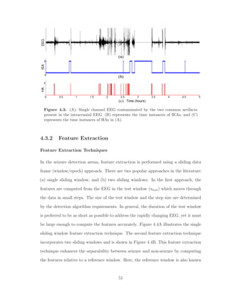
![as the background window (xbkg) that ideally represents the non-seizure EEG. The
background window can be fixed or slide synchronously with the test window. The
latter is more commonly used to ensure that the most current background EEG state is
used for the reference [51, 54]. The gap or separation between the test and background
windows reduces the chances of the background window to include seizure EEG. The
duration of the background window and gap is generally large compared to the test
window.
(A)
test window
xtest
(B)
step size test windowbackground window
xbkg xtest
gap
time
Figure 4.4: Feature extraction techniques: (A) single sliding window, and (B) two
sliding window feature extraction.
We experimented with different test window lengths (0.5-30 seconds) and selected
2 seconds to be suitable for the RFWE system. Detection delay and subtle changes
in the ongoing epileptic seizure are captured with a sliding test window that moves
in small steps. Empirically determined overlap of 75% is considered suitable for this
method. The test window is separated from the background window by a 60 s gap,
where the background window duration is chosen to be 30 s. The size of the gap and
the background window is taken from the previous studies of Gotman et al. [21, 32,
51, 54, 101, 156, 166].
52](https://image.slidesharecdn.com/039fdf0d-408b-485a-969c-4c8bab29d255-160116041507/85/RY_PhD_Thesis_2012-81-320.jpg)
![Relative Frequency-Weighted Energy
In general, seizure EEG patterns are distinguished from the background EEG by
a change in the amplitude in one or more dominant rhythms for a short duration.
However, some seizures show a fast transition in frequency with minimal or no change
in the amplitude. It is possible to quantify such seizures using frequency-weighted-
energy (FWE). Frequency-weighted-energy is sensitive to variations in both amplitude
and frequency resulting in higher energy during the seizure than non-seizure activity
[37, 39, 169]. Teager proposed a simple non-linear energy operator (NLEO) to quantify
the energy proportional to change in the amplitude or frequency. This operator can
be presented in its discrete form as [168]
ψ [x(n)] = x2
(n) − x(n − 1)x(n − 2), (4.1)
where x(n − k), k = 0, 1, 2 are delayed samples of the EEG signal. One of the key
properties of this operator for a pure sinusoid can be summarized by the rule
Ψ = ψ[A cos(ωin + φ)] = A2
sin2
(ωi), (4.2)
where A is the amplitude and ωi is the frequency. For ωi much less than the sampling
frequency, Ψ ≈ A2
ω2
i . In cases where the frequencies of interest are much lower than the
sampling frequency, as with EEGs, the output of NLEO can be considered a measure
of the spectral content of the signal [39, 167, 169-172]. A more generalized form of
the Teager operator had been given earlier by Plotkin and Swamy [170, 171, 172],
ψg[x(n)] = x(n − l)x(n − p) − x(n − q)x(n − s), l + p = q + s (4.3)
where ψg denotes generalized NLEO. Agarwal et al. [167] showed that for l = p and
q = s, ψg is more robust to noise. That is, if the input signal x contains additive
53](https://image.slidesharecdn.com/039fdf0d-408b-485a-969c-4c8bab29d255-160116041507/85/RY_PhD_Thesis_2012-82-320.jpg)
![white noise, then the output in Eq. (4.3) will not contain a component reflecting the
input noise [39, 167, 169]. This is due to the removal of the square term in Eq. (4.3).
For this reason, we choose l = 1, p = 2, q = 0 and s = 3. The expected value of the
output of the generalized NLEO (ψg) is referred to as the frequency-weighted-energy
(FWE) [39, 167].
Some seizures do not reflect any amplitude evolution, but show a rapid transition
from one frequency to another. FWE is useful in the identification of such seizures,
since it has been shown to be highly sensitive to amplitude and frequency changes
in the EEG [39, 167]. For this method, the feature is extracted using two sliding
windows. The ratio of the FWE in the two windows (test and background) is referred
to as the relative frequency-weighted energy, Q (n),
Q (n) =
1
N
N
1 ψg[xtest(n)]
1
M
M
1 ψg[xbkg(n)]
. (4.4)
An example of the time-evolution of a seizure in the RFWE is shown in Fig. 4.5.
Figure 4.5: The example represents 160 s of EEG activity that includes normal
(background) and seizure activity. The RFWE describes the changes seen in the EEG as
it progresses from inter-ictal (background) to ictal (seizure) state, and back to inter-ictal
state.
4.3.3 Classification
The RFWE feature shows a continual increase from the baseline at the onset of seizure,
as seen from Fig. 4.5. It was realized that this can be used to track the RFWE
54](https://image.slidesharecdn.com/039fdf0d-408b-485a-969c-4c8bab29d255-160116041507/85/RY_PhD_Thesis_2012-83-320.jpg)
![trajectory for a reliable seizure detection. However, sharp transients and artifacts
cause abrupt fluctuations in the time-evolution trends of the RFWE (Q [n]), and
must be addressed prior to classification. The spurious fluctuations in Q [n] can be
suppressed by a moving average (MA) filter to generate a smooth time-evolution trend.
Therefore, we incorporate a recursive moving average filter to attenuate the effects of
spurious fluctuations in Q [n], given by
Q[n] = Q[n − 1] +
Q [n] − Q [n − M]
M
, (4.5)
where Q[ ] is the M-point average output signal and Q [ ] represents the unfiltered
RFWE input signal.
We experimented with different lengths of the MA filter to determine the filter
length that best suits the RFWE system. Figure 4.7 illustrates the effect of the MA
filter length on the RFWE feature. It can be seen that with increasing filter length,
M, the spurious fluctuations in the Q [n] are suppressed, resulting in a smooth trend.
The amount of spurious noise reduced by the MA filter is equal to the square root of
the filter length. That is, a 120 points MA filter reduces the noise by a factor of 10.95
while a 360 point MA filter reduces the noise by a factor of 18.95 [173]. It is also noted
that a higher-order MA filter tends to blur the seizure onset and end. In the example
of Fig. 4.7, it can be seen that for M = 360 the envelop shifts the seizure onset and
terminates the seizure far beyond the actual seizure onset and end. Interestingly, the
output accurately maps the seizure onset and end for M = 120 points. After studying
the training data, a 120 points MA filter, which corresponds to 30 seconds of the EEG,
was considered suitable.
55](https://image.slidesharecdn.com/039fdf0d-408b-485a-969c-4c8bab29d255-160116041507/85/RY_PhD_Thesis_2012-84-320.jpg)
![Figure 4.6: Tracking the continual increase of the RFWE trajectory at the seizure
onset.
In the RFWE system, we aim to quantify the time evolution of the seizure to make
a detection that does not require a priori knowledge of the seizure type. In other
words, the method aims to track the continual increase in the feature value, which
does not require a default detection threshold with respect to the feature. However,
the definition of minimum duration of seizure can be used to control the trade-off
between sensitivity and specificity. This is achieved by examining the gradient of Q[n]
for continual increase as illustrated in Fig. 4.6. The gradient, ∆φ[n], is computed by
taking the difference of two successive Q[n] values.
∆φ[n] = Q[n] − Q[n − 1], (4.6)
Continual increase in the amplitude, frequency or both can be tracked using ∆φ[n]
by looking for a continual positive gradient. Furthermore, in order to classify the
continual increase in the RFWE trend to be due to seizure, it must satisfy a minimum
duration. This is achieved by extracting the sign of ∆φ[n] given by
56](https://image.slidesharecdn.com/039fdf0d-408b-485a-969c-4c8bab29d255-160116041507/85/RY_PhD_Thesis_2012-85-320.jpg)
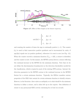
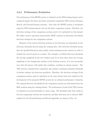
![Figure 4.8: ROC analysis for Grewal-Gotman system and Reveal algorithm. The
detection threshold of the Grewal-Gotman system and Reveal algorithm is varied from
1 to 10. The selected thresholds for Grewal-Gotman system (detection threshold = 3)
and Reveal algorithm (perception value = 5) are selected.
Note that the seizure varies from the patient-to-patient. Therefore, it is very
difficult to set a single threshold value at which the detector gives the best result
for all patients. One of our aims is to overcome this limitation, which we achieve by
tracking the time evolution of the seizure as it progresses.
Prior to any performance evaluation, all automatic detections that are within 30 s
of each other are clustered as a single seizure event. An event detected by the proposed
algorithm is considered a good detection, if there is any overlap with a manually
scored event; otherwise, it is considered a false detection. The performance is assessed
with the three most commonly used performance measures in the seizure detection
literature: sensitivity, specificity and false detection rate as described in Chapter 3
[32, 160].
59](https://image.slidesharecdn.com/039fdf0d-408b-485a-969c-4c8bab29d255-160116041507/85/RY_PhD_Thesis_2012-88-320.jpg)


![Figure 4.9: Seizure classification-based on duration.
Therefore, any spurious fluctuation in the RFWE feature is suppressed by a moving
average filter. Then, the gradient of the filtered RFWE is examined for a continual
increase to make a detection. An advantage of the RFWE system is that it does not
require a priori knowledge of seizures to set the detection threshold. Training-data
results demonstrate a significantly improved detection sensitivity over the NPS systems
in , [51], and [52] with a nearly similar detection specificity.
To better assess the limitations of the new NPS, we categorized the seizures based
on their duration and according to their characteristics upon visual review of the
training data. Seizure activity sustaining for more than 30 s were defined as long
seizures, otherwise they were considered short seizures. The distribution of short and
long seizures based on this classification is shown in Fig. 4.9. Patients 1, 2 and 5 had
both long- and short- length seizures, while Patients 3, 4, and 7 had only long-length
seizures and Patient 6 had only short-length seizures.
62](https://image.slidesharecdn.com/039fdf0d-408b-485a-969c-4c8bab29d255-160116041507/85/RY_PhD_Thesis_2012-91-320.jpg)
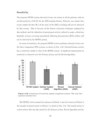


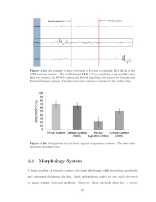
![short duration seizures or those with non-rhythmic mixed frequency characteristics
[32, 51, 100, 114, 88]. As noted in the previous section, a large number of false events
are detected in the presence of sharp transients and high-amplitude artifacts by the
proposed RFWE system as well as the three NPS systems selected for comparison.
This needs to be addressed in order to improve the overall detection performance for
widespread applicability of the NPS methods in the EMU.
In general, one common property of all epileptic seizures is the increase in the
number of sharp-wave complexes (SWCs) as the seizure progresses. Sharp wave com-
plexes include sharp transients, sharp waves and polymorphic epileptogenic waveforms
that are distinct from the background EEG [51, 174, 175]. Figure 4.17 illustrates the
evolution of epileptic seizure in the context of sharp-wave complexes (SWCs) as the
seizure progresses. By quantifying this unique morphological property of the EEG,
it may be possible to make more accurate seizure detections with improved system
performance. In our initial investigation of various EEG properties, we discovered that
sharpness of the half-waves (SHWs) can grossly characterize the EEG morphology.
It was noted that the number of SHWs profoundly increase as the seizure progresses.
This characteristic morphological property of the seizure is utilized to design a new
NPS system that we refer to as the morphology system [34, 120]. We note that this is
the first reported use of the sharpness feature to track temporal evolution of seizure
for detection.
The Morphology system is composed of the following six blocks.
1. Pre-processing and artifact rejection
2. Half-wave (HW) decomposition
3. Estimation of sharpness of the half-waves
4. Identification of sharp epileptiform activity
5. Median filtering
68](https://image.slidesharecdn.com/039fdf0d-408b-485a-969c-4c8bab29d255-160116041507/85/RY_PhD_Thesis_2012-97-320.jpg)

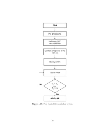
![4.4.2 Feature Extraction
Seizures occurring at the start of data recording are missed due to the unavailability of
the background EEG in the two sliding-window feature extraction scheme as observed
in the proposed RFWE system. Therefore, in this proposed system, the feature is
computed using a single window technique, i.e., no background EEG is utilized. A
small test epoch (0.5 s) is employed to capture subtle changes in the EEG to detect
seizure as close as possible to the onset.
Half-wave Decomposition
Majority of the false detections in the RFWE system and the three comparison NPS
systems were due to the discharge of sharp transients. These systems failed to make
a clear distinction between the seizure and sharp transients. As described earlier in
this section, one of the key properties of seizure is the persistent increase in the sharp
wave complexes (SWC) as the seizure evolves. By devising a method to quantify this
property, it is possible to improve the detection specificity. To do so, the EEG is
first decomposed into a series of half-waves, where a half-wave (HW) is defined as the
segment of EEG waveform located between two adjacent extrema (i.e., a minimum
and a maximum, or vice versa), as shown in Fig. 4.19. The extremas are detected
by the change in the sign of slope, which we measure as the difference between two
adjacent samples [22, 176]. To reduce the effect of small fluctuations due to noise and
artifacts, HWs less than 15 ms (3 samples) in duration are ignored.
Sharpness of a Half-wave
Each half-wave is characterized by its sharpness feature, sharpness being defined as the
slope (m) of the best-fit straight line of each half-wave. Since the slope is a function of
both amplitude and duration (frequency) of the HW, the sharpness feature is highly
sensitive to both of these. Some approaches in the literature have utilized the HW
71](https://image.slidesharecdn.com/039fdf0d-408b-485a-969c-4c8bab29d255-160116041507/85/RY_PhD_Thesis_2012-100-320.jpg)
![Figure 4.19: A section of EEG is zoomed in to illustrate half-wave decomposition and
estimation of sharpness of the half-wave. The slope of the best-fit line between the local
extrema (thick-black line) is the sharpness feature.
peak-to-peak amplitude and their duration as features for detection of epileptiform
EEG [22, 97, 110, 176]. In the same spirit, we quantify the amplitude and frequency
changes in the EEG by a single feature, the sharpness of the half-wave (SHW), defined
as the absolute value of m. It may be noted that this has not been previously reported
for the detection of epileptic seizures. The evolution of EEG sharpness as a function of
time is illustrated by the example in Fig. 4.20. Clearly, the SHW is profoundly greater
and increases during the seizure compared to that during the non-seizure activity. We
utilize this observation in the proposed morphology system to differentiate between
normal and epileptic activity.
72](https://image.slidesharecdn.com/039fdf0d-408b-485a-969c-4c8bab29d255-160116041507/85/RY_PhD_Thesis_2012-101-320.jpg)
![(a)
(b)
Figure 4.20: Evolution of SHW as the seizure progresses. (A) Seizure with background.
(B) SHW corresponding to the EEG in (A).
4.4.3 Classification
Identification of Sharp Epileptiform Activities
As noted in the example shown in Fig. 4.20, it is possible to discriminate between the
seizure and the normal EEG by applying a threshold that highlights abnormally sharp
activities linked with the seizure. This can be achieved by applying a scaled-heaviside
step function (activation function) [177] that limits the SHWs to a minimum sharpness,
and is given by
g(n) =
m for m ≥ mth
0 otherwise
, (4.8)
where mth is the threshold to identify candidate HWs that may correspond to the
seizures. Receiver operator characteristic (ROC) analysis on the training data is
73](https://image.slidesharecdn.com/039fdf0d-408b-485a-969c-4c8bab29d255-160116041507/85/RY_PhD_Thesis_2012-102-320.jpg)
![utilized to determine the default value of mth that provides a suitable separation
between seizure and non-seizure EEG. Using the MNI training data, the sensitivity
and the FDR are computed for each mth in the range of 5 − 50. We use the knee of
the ROC curve to select mth and is shown in Fig. 4.21.
Median Filter
The output of the activation filter is shown in Fig. 4.22C, which indicates that not all
sporadically occurring SWCs in the EEG (see Fig. 4.22C prior to seizure onset) are
removed. Such occasionally occurring SWCs may lead to an increase in the detection
of false events. Therefore, such sporadic SWCs must be removed prior to classification.
The impact of spurious SWCs can be suppressed or smoothed by a moving average
or a median filter. A median filter is preferred to eliminate the effect of a few SWCs
over the moving average filter, since it is insensitive to outliers and the extreme values
[100, 129, 178, 179].
The median filter is defined as follows: To compute the output of a median filter,
an odd number of sample values are ranked (sorted numerically) and the middle value
is used as the filter output. For a filter of window length (L = 2k + 1), the filtering
procedure for the input SHW sequence is given by
G(n) = med[g(n − k), . . . , g(n), . . . , g(n + k)] (4.9)
where g(n), and G(n) are the input values and the output of the window centered at
the nth value, respectively. In Eq. (4.9), ’med’ denotes the median value. Equation
(4.9) represents a non-recursive median filter [178, 180]. Computational cost can be
reduced by employing a recursive median filter that replaces the center point g(n) of
the window by the median value of all the points inside it, and uses these values to
calculate the median in the subsequent window positions. The output of recursive
median filter is given by
74](https://image.slidesharecdn.com/039fdf0d-408b-485a-969c-4c8bab29d255-160116041507/85/RY_PhD_Thesis_2012-103-320.jpg)
![G(n) = med[G(n − k), . . . , G(n), g(n), . . . , g(n + k)], (4.10)
which replaces at every step, the leftmost k-points in the moving window with the
previously k output points [181, 180]. The filter length (L) is empirically determined
considering the low-frequency seizure activity. We hypothesize that each 0.5-second
epoch will have at least one abnormally sharp activity, therefore, a total of 12 in the
six seconds, we round this number to 15 for robustness due to potential influence by
noise.
An added advantage of this layer is that it preserves continual increase of the
SHWs as the seizure evolves. Figure 4.22 illustrates the process of quantifying SWCs
using half-waves. In this example, a 10 s section of epileptic seizure is shown in Fig.
4.22A, and best-fit straight lines for each HW are shown in Fig.4.22B. The sharpness
measure (m) of the HWs that satisfy the requirement for SHWs are shown by the bar
plot in Fig. 4.22C. G(n) clearly reveals absence of SHWs prior to seizure onset while
during the post onset there is sudden increase in the number of SHWs (Fig. 4.22D).
Figure 4.21: Threshold estimation using the receiver operating characteristics (ROC)
analysis. The threshold mth is varied from 5 to 50 and for each mth, the average
sensitivity and false detection rate is computed to generate the ROC curve. The default
threshold (mth = 25) which we use for morphology system is shown encircled.
75](https://image.slidesharecdn.com/039fdf0d-408b-485a-969c-4c8bab29d255-160116041507/85/RY_PhD_Thesis_2012-104-320.jpg)
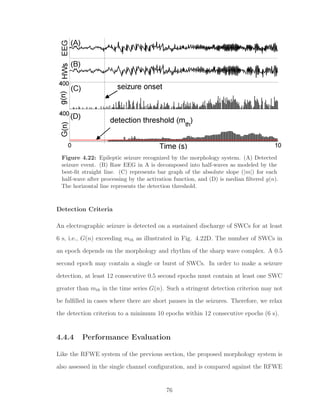
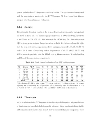

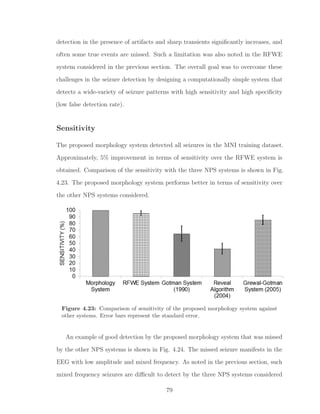
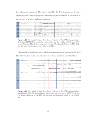
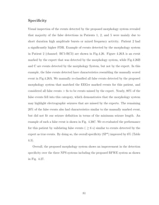
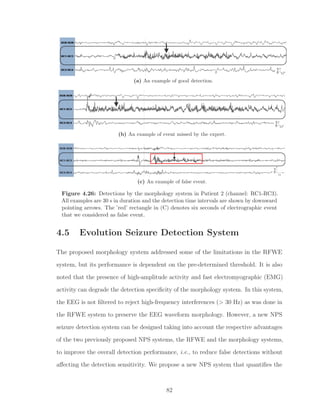
![Figure 4.27: Comparison of specificity of the morphology system with the other
systems on the MNI training dataset. Error bars represent standard error.
evolving changes in the EEG characteristics as the seizure progresses, and will be
called the evolution seizure detection (eSD) system [33, 136].
The seizure identification in the proposed eSD system is done in two steps. The
concept utilized in the eSD system is to first identify candidate seizure (CSZ) events
based on the evolving changes in the amplitude, frequency and the rhythmicity, and
then verify the CSZ event sharpness characteristics to make the final detection. The
proposed eSD system scheme gains its strength from (a) a novel computationally
simple scheme, which continuously examines the evolving characteristics of the EEG
features to set unique detection threshold to identify the candidate seizure event, and
(b) then use a computationally simple approach to validate and classify the candidate
seizure event. The proposed eSD system is composed of the following four blocks.
1. Pre-processing and artifact rejection
2. Feature extraction
3. Identification of candidate seizure event
4. Validation of candidate seizure event
83](https://image.slidesharecdn.com/039fdf0d-408b-485a-969c-4c8bab29d255-160116041507/85/RY_PhD_Thesis_2012-112-320.jpg)


![Sharp-Wave Complex Density
One of the key properties of seizure evolution is the continual increase in the number
of sharp components, as previously discussed in Section 4.3 [34]. Patterns due to
artifacts can be isolated by examining this characteristic property of seizure evolution.
We compute the SWC density feature to establish the increase in the number of
sharp components as the seizure evolves. This is achieved by decomposing the EEG
into half-waves and quantifying the sharpness of the half-waves by the slope of the
best-fit line, as was done in the morphology system in Section 4.4. As was done in
that system, the sharpness of the half-waves is restricted to highlight the potential
epileptiform sharp activity. The SWC density (SWCD) is then defined as the number
of SHWs in the test epoch. Computational load can be significantly reduced by
computing the density of SWCs in a non-overlapping test window instead of a sliding
window that moves in small steps. Therefore, the density of SWCs is computed from
a two-second non-overlapping test window. This feature is computed along with the
other three features, but used only to validate a candidate seizure event (CSZ). The
validation of CSZ involves establishing evolving changes in terms of sharp-components
to differentiate between seizure and artifact.
Coefficient of Variation of the Amplitude
The coefficient of variation of the amplitude (CVA) quantifies in a simple way the
increased regularity in the amplitude during a seizure. It is defined as the ratio of
variance of the absolute amplitude to the square of the mean absolute amplitude.
CVA=
σ2
|xtest|
µ2
|xtest|
, (4.11)
where σ2
|xtest| is the variance and µ|xtest| is the mean of the absolute of the xtest. The
CVA is computed from the 2 s test epoch that slides in small steps. Signals exhibiting
87](https://image.slidesharecdn.com/039fdf0d-408b-485a-969c-4c8bab29d255-160116041507/85/RY_PhD_Thesis_2012-116-320.jpg)
![strong rhythmic characteristics are likely to have regularity both in the frequency
and the amplitude as typically observed in the seizures [32]. An example of CVA
feature before and after a seizure onset is shown in Fig. 4.29. The CVA decreases
with the increased rhythmic EEG activity and vice versa. It is seen in Fig.4.29 that
CVA decreases and remains below some arbitrary baseline value during the seizure.
-20 -10 0 10 20 30 40
Time (s)
Onset
Figure 4.29: Time evolution of coefficient of variation of amplitude superimposed on
the EEG.
Relative Amplitude
The widely accepted definition of epileptic seizure states that during an epileptic
seizure, a new type of EEG rhythm appears, hesitantly, and then more distinctly, and
soon it boldly dominates the EEG tracing. It tends to become slower with increasing
amplitude and the more distinct spiky phases of the rhythmical waves appear [5].
Our observation is consistent with this definition with respect to the increase in the
amplitude relative to the background during a seizure evolution, and is therefore,
considered as one of the hallmark features suitable for the identification of seizures.
The relative amplitude (RA) is computed using the two sliding window technique. It
is defined as the ratio of the mean absolute amplitude in the test window (xtest) and
the background window (xbkg) and is given by
RA =
E(|xtest|)
E(|xbkg|)
, (4.12)
88](https://image.slidesharecdn.com/039fdf0d-408b-485a-969c-4c8bab29d255-160116041507/85/RY_PhD_Thesis_2012-117-320.jpg)
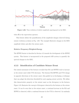
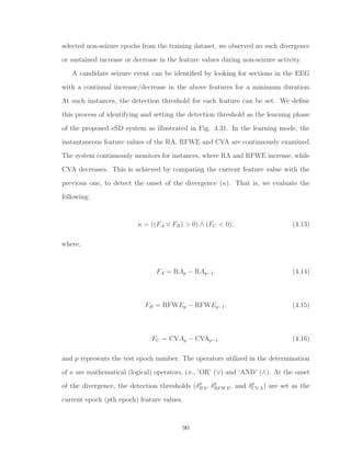
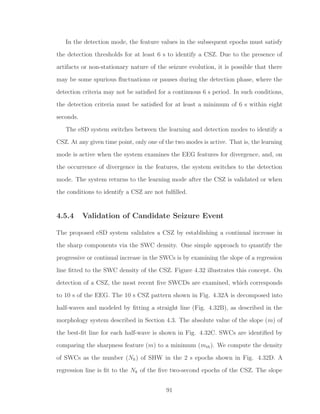
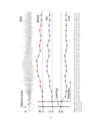
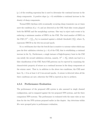
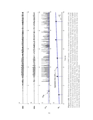
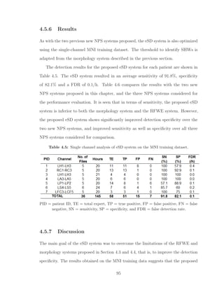
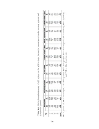
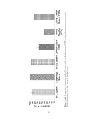
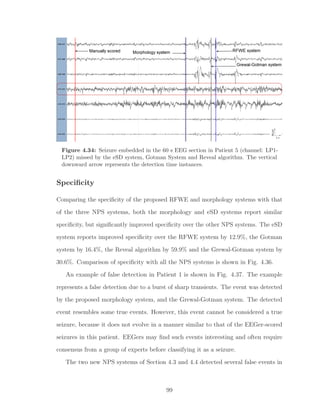
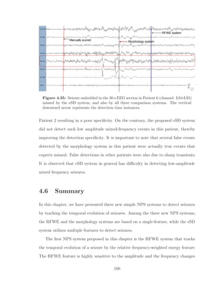
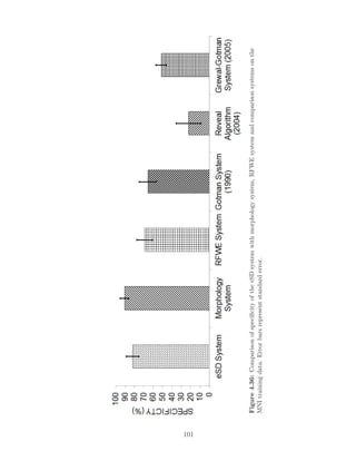
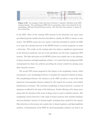
![Chapter 5
Performance Evaluation and Rapid
EEG Review Tool
5.1 Introduction
Three new NPS seizure detection systems were proposed and optimized using the MNI
training dataset in Chapter 4. In this Chapter, we evaluate the performance of these
new systems on a previously unseen MNI test dataset. Among the three proposed
NPS systems, the one with the best performance is selected for final performance
assessment on a completely blind test data (FSP database). We conclude this chapter
by demonstrating a novel tool to aid in a rapid review of voluminous multichannel
EEG recordings for application in EMU [119, 182].
5.2 MNI Database Results
In Chapter 4, we proposed three new NPS systems and presented results on the
seven patients (Patients 1-7) belonging to the training dataset of the MNI database.
We compared the performance of the new NPS system against three popular NPS
systems from the literature. Training data results of the new systems revealed an
104](https://image.slidesharecdn.com/039fdf0d-408b-485a-969c-4c8bab29d255-160116041507/85/RY_PhD_Thesis_2012-133-320.jpg)

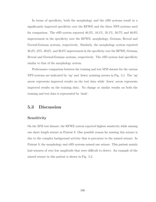
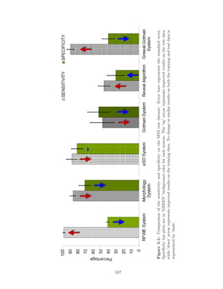
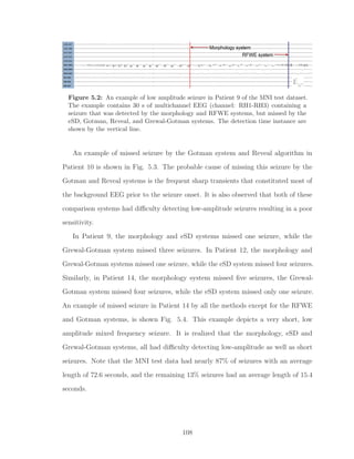
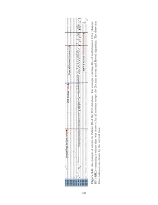
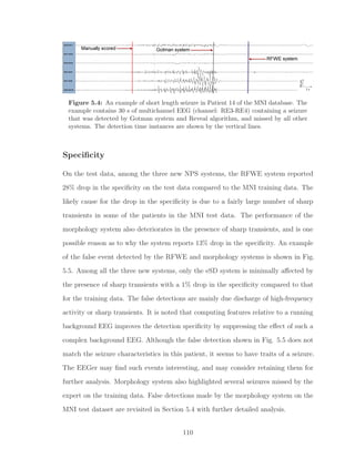
![Figure 5.5: An example of false detection in Patient 9 of the MNI test data. The
example contains 30 s of multichannel EEG (channel: RH1-RH3) detected by RFWE
system and morphology system, but not by other NPS systems. The detection time
instances are shown by the vertical lines.
5.4 FSP Database Results
The performance assessment on the MNI test data can still be viewed as biased for
several reasons. Since the proposed methods were developed in sequence, after the
assessment of first method, that test data is no longer blind to subsequent methods
even though the test data was not used in the development of the other methods.
Our channel selection criterion and single channel vs. multichannel performance
evaluation are among several possible reasons. Depth recordings are made using the
grid, strip or depth electrodes. The strip and grid electrodes are disk electrodes of
4 mm in diameters that are placed on brain surface (cortex). On the other hand,
depth electrodes penetrate the brain and have multiple electrodes along their length
with smaller surface area compared to the grid and strip electrodes. They may be
closer to the generators of the epileptic discharges and hence, the EEG may be of
higher amplitude. Thus, electrode configuration can cause variations in the overall
system performance [47, 183]. In addition, the digital EEG acquisition systems within
the same center and across different EMUs, have different front-end settings such as
amplifier gains, filter settings and sampling rates. These settings can also lead to
variation in the performance. Therefore, we evaluate the performance of one of the
new NPS systems proposed in Chapter 4, and compare it with one of the popular
comparison NPS systems, on a totally new EEG dataset recorded using a different
111](https://image.slidesharecdn.com/039fdf0d-408b-485a-969c-4c8bab29d255-160116041507/85/RY_PhD_Thesis_2012-140-320.jpg)
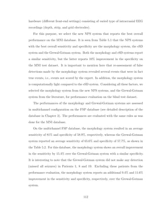
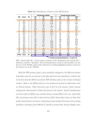
![properties of the seizures. False detections are clearly non-seizure like activity. Two
neurophysiologists (EEGer A & B) independently re-assessed all the false detections,
and classified them in the above three categories for the proposed morphology system
and the Grewal-Gotman system. We define the three category classification of the
FDs by the experts as Assessment I. The performance is re-assessed using Assessment
I approach and the results are shown in Table 5.3. Re-assessment of the FDs for the
two methods showed improvement in the specificity for all data.
It is not uncommon to note variability in the EEG scoring by the experts. We too
note a variation in the EEGer scoring. Therefore, we estimated the Cohen’s κ score,
a popular measure employed to measure inter-rate variability. We used κ statistics
to adjust the observed inter-observer agreement (po) for the proportion of random
agreement (pe): κ = (po − pe)/(1 − pe). If both the EEGers are in complete agreement,
then κ = 1. If there is no agreement other than what would be expected by chance,
then κ ≤0 [116, 184]. A moderate agreement between the two EEGers is achieved
(κ = 0.43) on re-assigning these false detections into the three categories (SL, IE, and
FD).
Some EEGers consider classifying the EEG into two categories: seizure-like and
false detection [52, 185]. This motivated us to evaluate the performance using the
two category classification, which we define as Assessment II. In this assessment of
false detections, we combine the seizure-like and interesting as seizure-like events.
The specificity for the Assessment II validation approach is also shown in Table
5.3. Re-assessment using Assessment II showed an improvement in the detection
specificity for the two systems. This classification mode resulted in a substantial
agreement (κ = 0.81) between the EEGers, establishing expert’s agreement on a
clear demarcation between the two categories: SL and FD. Re-assessment of the false
detection is discussed in the next section.
114](https://image.slidesharecdn.com/039fdf0d-408b-485a-969c-4c8bab29d255-160116041507/85/RY_PhD_Thesis_2012-143-320.jpg)
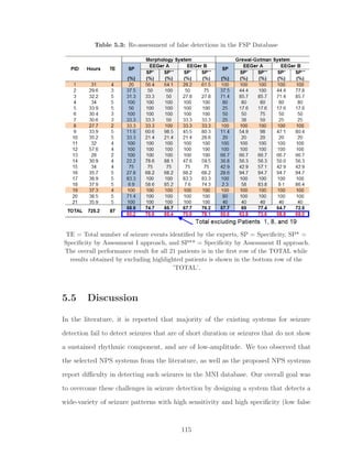
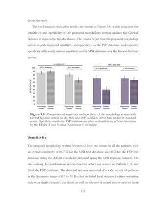
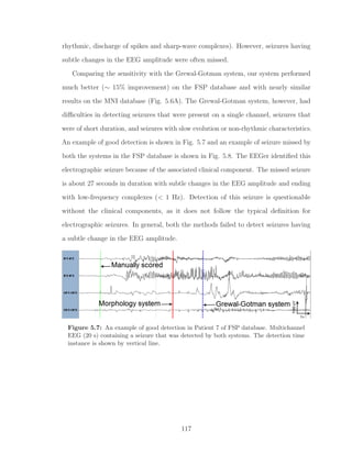
![Figure 5.8: An example of missed event in Patient 5 of FSP database. Multichannel
EEG (20 s) containing a seizure that was missed by both systems. The detection time
instance by EEGer is shown by the dotted vertical line.
Specificity
As previously mentioned, specificity indicates the quality of detections made by the
seizure detection method. On the MNI database, using the default threshold, the
morphology system had an average specificity of 91.2 % on the training data [34]
and 71.3% on the test data. A specificity of 58.9% is obtained on the FSP test
database. The specificity on the FSP test database is poor compared to that on the
MNI database, thus indicating a higher false detection rate. It is possible that some
of these false detections may in fact be sub-clinical seizures that were not identified by
the EEGer in the original review of this data. Re-evaluating these false detections
may provide more insight into the detection specificity.
The average number of false detections in the MNI database as well as in the
FSP database were quite uniform in majority of the patients. In the MNI database,
two patients (Patient 9 and 11) had a significantly large number of false detections.
In both cases, majority of the false detections occurred prior to the seizures. The
false detections included a discharge of sharp-wave complexes (∼5 s), low amplitude
fast activity, or were due to bursts of sharp transients in addition to high amplitude
artifacts (see Fig. 5.9). A large proportion of the false detections occurred several
seconds to several minutes before the seizure onset. A recent study by Marsh et al.
118](https://image.slidesharecdn.com/039fdf0d-408b-485a-969c-4c8bab29d255-160116041507/85/RY_PhD_Thesis_2012-147-320.jpg)
![[45] has demonstrated the role of interictal epileptic discharge (IED) for improved
localization of seizure focus in children with intractable epilepsy. The authors report
that electrodes with highest frequency of IEDs over long periods of intracranial EEG
correlate with the electrodes involved in the seizure onset in about two-thirds of
patients [45]. Furthermore, IEDs are used clinically in a variety of ways to help
identify the regions of surgical resection [186]. Several other studies, using long-term
depth EEG, report that in addition to resection of the seizure onset zone, resection
of regions generating ’significant’ interictal spikes and sharp waves improves seizure
freedom postoperatively [187, 188]. It may be possible that in some patients increased
false detections by our system, due to increased sharp activity, are precursors to
seizures or markers for seizure onset zones. Therefore, such events can be potentially
used as a clinical tool to identify regions of interest that warrant further review.
Similarly, a large proportion of false detections in the FSP database were due
to discharges of sharp-wave complexes and fast rhythmic activities. Two patients
(Patient 9 and 18) had a significantly higher number of false detections. An example of
false detection for Patient 9 is shown in Fig. 5.10 and for Patient 18 in Fig. 5.11. The
examples in Fig. 5.10 and 5.11 in fact resemble sub-clinical electrographic seizures that
were not marked by the EEGer. As noted above, this is because the FSP database is
annotated by experts based on the knowledge of clinical seizures. That is, the data was
reviewed for the presence of electrographic discharges only at the instances of clinical
seizures. It is possible that some of the false detections (EEG sections without clinical
events) are indeed electrographic seizures. To further evaluate these false detections,
two neurophysiologists (EEGer A and B) re-classified these events into three categories
(Assessment I), seizure-like (SL) activity, interesting events (IE) and false detections
(FD). Seizure-like activity included detections that matched characteristics of seizures
(as in, Fig. 5.10 and 5.11). Interesting events included detections such as discharge
of sharp transients that may be considered interesting events to the EEGer. False
119](https://image.slidesharecdn.com/039fdf0d-408b-485a-969c-4c8bab29d255-160116041507/85/RY_PhD_Thesis_2012-148-320.jpg)

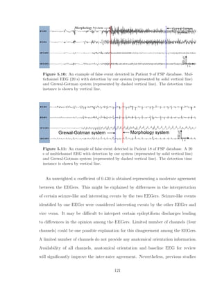
![have shown that EEGers (based on their experience) report perfect to near perfect
agreement when the EEG is categorized into seizure and false detections [116, 184, 189].
In our data, near perfect agreement (κ = 0.81) between the EEGers is achieved when
all events that were scored seizure-like by one EEGer and interesting by the other
are treated as true positives, i.e., the two categories (seizure-like + interesting =
seizure-like) are combined. Therefore, we computed specificity for two category re-
classification (Assessment II). As expected, an overall improvement in the specificity
is observed (see Table 5.3 and Fig. 5.12), which suggests that several FDs are in fact
seizures that were not originally scored in the FSP database.
It can be seen that the specificity is poor in some patients in both the MNI and
FSP databases. That is, there are a large number of false detections in these patients
due to short paroxysmal activities. For clinical application of the method, a tunable
threshold must be considered, which can be used to address the trade-off between the
detection sensitivity and specificity. In our NPS systems, we have aimed to remove
the dependence on the preset detection thresholds. However, the use of a minimum
duration as part of the definition of seizures can be considered as a threshold that
can be tunable. The EEGer can increase the duration threshold on observing a large
number of short false events to reduce these false detections.
It is important to mention here that MNI database are all depth recordings while
FSP database is a mix of depth, strip and grid recordings. Seizure manifestations
in the depth EEG are likely to be similar for both the databases, while strip and
grid electrodes are likely to have a different manifestation. This is because seizure
manifestation is different for different brain regions. Depth electrodes can be placed
into deeper brain regions such as hippocampus, hypothalamus, and deep frontal lobes,
where there is inadequate coverage provided by subdural strip and grid electrodes.
Furthermore, the two database were acquired using two different hardware (Stellate
Harmonie and Neurofile NT systems) and at two different sampling rates. The
122](https://image.slidesharecdn.com/039fdf0d-408b-485a-969c-4c8bab29d255-160116041507/85/RY_PhD_Thesis_2012-151-320.jpg)
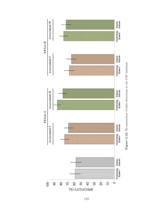
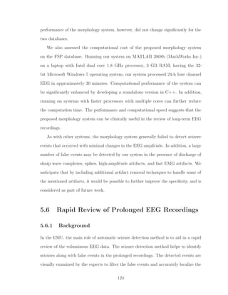
![epileptogenic sites, which is a tiresome task. Mapping channel-by-channel timeline of
seizures and the epileptiform activities can provide visualization of seizure onset and
spread (both temporally and spatially), and can be a powerful tool for planning of
surgical resection. This type of 2D visualization is generally unavailable for the review
of intracranial EEG. Therefore, it becomes very important to develop adjunctive
tools that allow quick identification of seizures, provide a view of seizure activity over
prolonged durations, seizure recurrence frequency, and the sites involved in the seizure
generation for therapeutic interventions and management [5, 38-41].
Rapid identification of epileptogenic sites and evaluation of spatio-temporal dynam-
ics is possible by digital trending tools [38-40]. Tools such as amplitude integrated
EEG (aEEG ), envelope trend (ET), compressed spectral array (CSA), color density
spectral array (CDSA), and compressed EEG pattern analysis (CEPA) allow graphical
display of the EEG trends [38-40]. The process typically involves splitting EEG data
into small epochs, and extracting features for graphical display. For example, CSA
displays time, frequency, and power in a three-dimensional graphical view. However,
CSA display has a practical limitation of a few channels [38, 40, 42, 190]. CDSA is a
modified CSA that allows the display to accommodate a few more channels. Typically,
intracranial EEG recording consist of 32 to 256 channels. The large number of channels
increases the computational complexity. EEGer experience in the interpretation of
such graphical display is yet another limiting factor [38-40]. These factors limit the
utility of the compressed EEG display in the EMU. Computationally simple and
easy-to-interpret compressed EEG display, specially designed to review multichannel
intracranial EEG for paroxysmal or seizure activity is much needed.
5.6.2 Method
Note that the seizure onset zone is the single most definitive localizing feature of the
epileptogenic region. For this reason, it is important to identify all channels (electrodes)
125](https://image.slidesharecdn.com/039fdf0d-408b-485a-969c-4c8bab29d255-160116041507/85/RY_PhD_Thesis_2012-154-320.jpg)
![in the seizure onset and their recurrence frequency for anatomical localization [38-40].
As previously mentioned in Chapter 4, an electrographic seizure is a discharge of
sharp wave complexes evolving in frequency and amplitude, including repetitive spikes.
Furthermore, discharge of sharp waves (sharp transients, spikes, and epileptiform
discharges) occur more frequently than seizure, and can be linked to the brain regions
involved in the epileptogenesis [5]. It is realized that the sharpness of the EEG
waveform can be a robust marker to highlight epileptogenic areas (both temporally
and spatially). The sharpness measure to parametrize the EEG waveform morphology
proposed in Chapter 4 is utilized to generate the new compressed display.
Easy, reliable and intuitive interpretation is important to maintain patient safety
in the EMU, where experienced EEGer may not be available round-the-clock. Color-
intensity plots are intuitive, easy-to-interpret and require minimal training. Therefore,
we quantify the level of sharp activity in the EEG, and graphically display it as a color-
intensity plot. To do so, we split the EEG into short segments (epochs) and extract
a feature for the graphical display. For compressed display, the EEG is processed in
10 s non-overlapping epochs. The feature for graphical display is the level of sharp
activity in an epoch referred to as relative sharpness index (RSI), and is given by
RSI =
# of m > mth
Total # of m
, (5.1)
where m is a measure of the sharpness of the half-waves in the epoch (see Chapter
4, Section 4.4). The resulting RSI is displayed as a color-intensity plot that allows
the compression of several hours of multichannel EEG on a single page display. We
randomly selected two patients from the MNI database to illustrate the RSI display
to aid in a rapid review of prolonged intracranial EEG recordings.
126](https://image.slidesharecdn.com/039fdf0d-408b-485a-969c-4c8bab29d255-160116041507/85/RY_PhD_Thesis_2012-155-320.jpg)
![5.6.3 Results and Discussion
The performance evaluation of the compressed displays is done by examining the
display size, interpretation, and computational complexity. To do a comparative
assessment of these complexities, we selected CDSA and aEEG displays. Compressed
EEG displays using all three techniques (RSI, CDSA and aEEG) were generated for
the two patient EEG recordings from the MNI database. Seizure, epileptiform activity,
and areas of potential seizure development were visually identified and correlated with
the EEG. This evaluation allowed us to decide on the best method among the three
techniques.
13:39 13:49
F
0
0.2
0.4
0.6
0.8
1
30
0
TIME [HH:MM]
COLOR DENSITY SPECTRAL ARRAY (CDSA)
COLORMAPRELATIVE SHARPNESS INDEX (RSI)
Figure 5.13: Identification of seizure in the compressed EEG display. The example
represents 10 min single channel RSI and CDSA displays. Seizure detected by the EEGer
is annotated with ’horizontal bar’ on both the displays.
First, it is important to describe how compressed displays are interpreted for
seizures. Note that compressed display represents EEG activity in a transformed
domain as a function of time. The features utilized are the level of sharpness in the RSI
display, power at the different frequencies in the CDSA, and the amplitude activity
in the aEEG. These features are represented as color-intensity (RSI and CDSA) or
trend (aEEG) graphs. An electrographic seizure evolves in both the amplitude and
frequency; therefore, the intensity or the magnitude of the feature will be lower during
non-seizure and maximum during a seizure. A seizure can be identified by looking
for high-intensity segments in the compressed display. An example to illustrate the
127](https://image.slidesharecdn.com/039fdf0d-408b-485a-969c-4c8bab29d255-160116041507/85/RY_PhD_Thesis_2012-156-320.jpg)
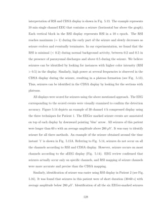
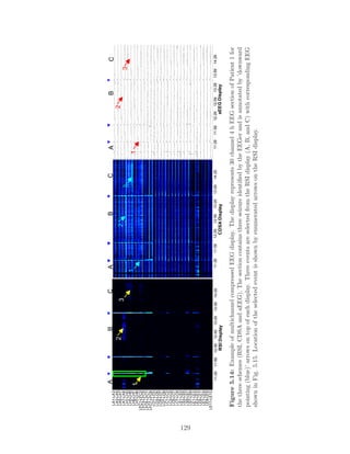
![13:15:1413:15:1913:15:2413:15:2913:15:3413:15:39
LFC3-LFC5
LFC1-LFC3
LH7-LH8
LH5-LH7
LH3-LH5
LH1-LH3
LA7-LA8
LA5-LA7
LA3-LA5
LA1-LA3
11:33:4411:33:4911:33:5411:33:5911:34:0411:34:09
LFC3-LFC5
LFC1-LFC3
LH7-LH8
LH5-LH7
LH3-LH5
LH1-LH3
LA7-LA8
LA5-LA7
LA3-LA5
LA1-LA3
14:31:5414:31:5914:32:0414:32:0914:32:1414:32:19
LFC3-LFC5
LFC1-LFC3
LH7-LH8
LH5-LH7
LH3-LH5
LH1-LH3
LA7-LA8
LA5-LA7
LA3-LA5
LA1-LA3
A
TIME[HH:MM:SS]
C
B
EEGREVIEWPANEL
Figure5.15:EEGcorrespondingtotheeventsselectedfromtheRSIdisplayinFig.5.14.(A)representsaseizurearoundthetime
point’1’,(B)representsthepre-ictalrhythmicdischargeofsharpwavesaroundthetimepoint’2’,and(C)representsdischargesof
sharpwavecomplexesaroundthetimepoint’3’inFig.5.13,respectively.Eachsegmentrepresents30sof10channelEEG.
130](https://image.slidesharecdn.com/039fdf0d-408b-485a-969c-4c8bab29d255-160116041507/85/RY_PhD_Thesis_2012-159-320.jpg)
![using CDSA and aEEG was difficult. This is probably due to the fact that seizures in
this patient were focal and low amplitude (channel: RH1-RH2 and RC1-RC2). This is
consistent with the observations in [5, 191]. As with the CDSA and aEEG, detection of
seizures with no or minimal change in the EEG amplitude (< 20 µV) is also challenging
for the RSI display. However, RSI is still able to clearly and accurately highlight the
epileptogenic sites, i.e., channels with profoundly increased sharp activity (confirmed
by the EEG review) than the comparison displays. Increased sharp activities are
often associated with regions involved in the seizure generation [190]. Therefore, this
information may be clinically vital in the identification of neuronal areas involved
in the seizure generation. In Patient 1, we observed such activity to be present,
predominantly and consistently in all seizure EEG sections on the channels LA7-LA8,
LFC1-LFC3 and LE2-LE3 (see Fig. 5.14) that disappears at the seizure onset. The
corresponding raw EEG of such an activity is shown in Fig. 5.15B (obtained around
the time instant shown by arrow ’2’ in Fig. 5.14). In this patient, RSI display also
reveals increased sharp activity on other sites as well (channel: LH1-LH3, LH3-LH5
and LH7-LH8). Figure 5.15C depicts an example of such activity (around the time
instant shown by arrow ’3’ in Fig. 5.14). Similarly, in Patient 2, such sharp activity
predominantly occurs only on two specific channels (RH1-RH2 and RC1-RC2) as seen
in Fig. 5.16 (RSI display). CDSA display also confirmed presence of such activity but
not the aEEG display (not shown).
A compressed display is advantageous in the EMUs when timely intervention
becomes important on seizure detection to prevent secondary brain damages [5, 38, 39,
192]. The main limiting factor of the compressed display is the display-size complexity
[38, 193]. In CDSA and aEEG, the spatio-temporal resolution of the display decreases
with an increase in the number of channels and the duration of monitoring, making
the interpretation very difficult. On the contrary, an increase in the number of
channels minimally affects the RSI display. This effect can be seen on the multichannel
131](https://image.slidesharecdn.com/039fdf0d-408b-485a-969c-4c8bab29d255-160116041507/85/RY_PhD_Thesis_2012-160-320.jpg)
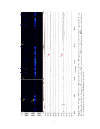
![that removing the latter two dependencies would lead to a more practical solution in
the design of PS systems.
In Chapter 1, we introduced the framework of a fully automatic PS system that
aims to address the existing challenges in the seizure detection by combining the NPS
and PS systems. New computationally light NPS systems were developed in Chapter
4 and 5 for this framework. In this chapter, we develop a new PS seizure detection
system that eliminates the need for supervised selection of non-seizure data and for
the supervised training of the classifier. Such a PS system is able to detect recurring
seizure patterns of non-equal duration. The new PS system builds a seizure model
for a previously identified seizure that can be used with the statistically optimal null
filter (SONF) for subsequent detection of similar seizures [37, 134, 135, 194]. The
performance of the new PS system is evaluated on the 304 h of single channel EEG
obtained from 14 patients of MNI database and is compared with the clinically used
PS system proposed by Qu and Gotman [21].
6.2 Problem Formulation
We assume seizure to be a narrow-band signal in comparison to the disproportionately
large background EEG and define the problem as the detection of rhythmic narrowband
seizure activity, s(n), from the observed EEG consisting of signal and noise, x(n) =
s(n) + n(n). It is important to note that the rhythmic narrowband seizure activity
evolves as the seizure progresses over time. In other words, a seizure is composed
of short piecewise stationary rhythmic discharges that change from one rhythm to
another as the seizure progresses. Figure 6.1 illustrates the temporal progression of a
seizure in short piecewise stationary rhythms. The problem can be re-defined as the
detection of these narrowband piecewise stationary rhythms, i.e., the template seizure,
s(n), consisting of a set of components, s1(n), s2(n) , ... sN (n), with a specific order of
136](https://image.slidesharecdn.com/039fdf0d-408b-485a-969c-4c8bab29d255-160116041507/85/RY_PhD_Thesis_2012-165-320.jpg)

![seizure and non-seizure. We select statistically optimal null filters (SONF) for the
proposed model-based PS system. The use of SONF is a novel approach for the prob-
lem of enhancement/suppression of narrowband signals of short-record length based
on combining maximum signal-to-noise ratio (SNR) and least-square optimization
criteria [170, 172]. Its intrinsic property is the ability to track signals rapidly leading
to a more practical processing of short-duration signals and has been shown to be
equivalent to the well-known Kalman filter, but with a much simpler implementation
[195-199]. SONF is a linear time-varying filter, and can be implemented as a number
of parallel filters. Thus, SONF becomes an obvious choice for processing time-varying,
narrowband seizure components that may lead to a practical PS system. However,
SONF requires a priori knowledge of the signal components or the basis functions
constituting the signals to be estimated.
In the proposed PS system, the first step involves partitioning the seizure signal
s(n) into a set of piecewise stationary seizure components, s(n), s2(n), ..., sN (n). Here,
an a priori known seizure is considered as the template seizure pattern TPAT , the
piecewise stationary segments as seizure components or epochs, and the unknown
seizures for a given patient as the candidate seizure pattern (CPAT ). The second step
involves extracting ’k’ non-redundant rhythmic components of TPAT that constitute
the set of ’template epochs’. The third step involves identifying the composing basis
functions for each template epoch that are required to implement the SONF. The
seizure model is a set of basis functions for each of the k-template epochs. Finally,
the PS classifier is trained using TPAT and the derived seizure model. The trained
PS system is employed to detect narrowband template epochs in all subsequent data.
The tracking of the time-ordered occurrence of k-template epochs is possible by a
parallel implementation of the SONFs, where each of the SONFs corresponds to a
different template epoch of TPAT . That is, at any given time only one SONF will track
a template epoch. By tracking the time-ordered estimation of the components by the
138](https://image.slidesharecdn.com/039fdf0d-408b-485a-969c-4c8bab29d255-160116041507/85/RY_PhD_Thesis_2012-167-320.jpg)
![SONF, it is possible to identify the subsequent seizures with similar characteristics.
An added advantage of this detection strategy is the ability to minimize the detection
of non-epileptic rhythms that have similar rhythmic characteristics as TPAT , but not
the time-ordered component occurrence. This is due to the fact that the dominant
rhythm of an epileptic seizure evolves in short bursts as shown in Fig. 6.1, while
normal EEG rhythms do not typically evolve. The non-epileptic rhythms include the
non-ictal rhythmic discharges such as the alpha rhythms, mu rhythms, lambda waves,
sleep spindles, and sub-clinical rhythmic discharges (SREDA) [5, 134].
6.3 Model-Based Seizure Detection
The block diagram of the proposed PS system is shown in Fig. 6.2, and consists of
the blocks: (a) pre-processing and artifact rejection, (b) seizure model, (c) SONF,
(d) detection criterion (energy ratio), and (e) evolution-based classification. SONF is
used to estimate the seizure waveform (rhythmic components) from the observed EEG.
If the observed EEG contains the same type of seizure as described by the a priori
known model, the output of the SONF will represent an estimate of the seizure ˆs(n).
In this case, the energy ratio γ between the seizure estimate ˆs(n) and the observed
EEG x(n) should be large; conversely, if the EEG contains no seizure (x(n) = n(n)),
then the SONF output should be near zero with little energy. The energy ratio in
this case will be small. Thus, the energy ratio γ of the seizure estimate ˆs(n) and the
observed EEG x(n) can be used as a metric to decide whether the input EEG contains
a seizure or not [132]. In terms of k-parallel SONFs, one for each of the k-template
epochs, the energy ratio γk of the estimate of the kth template epoch, ˆsk(n), and the
observed EEG x(n) is used as a metric to decide whether the input EEG contains the
kth template epoch or not. The time-ordered sequence in which the template epochs
occur in the TPAT and CPAT are matched to determine whether the TPAT and CPAT
139](https://image.slidesharecdn.com/039fdf0d-408b-485a-969c-4c8bab29d255-160116041507/85/RY_PhD_Thesis_2012-168-320.jpg)
![are similar or not.
As previously mentioned, the first step in building the seizure model involves
segmenting the template seizure pattern (TPAT ) into stationary epochs (piece-wise
stationary rhythms as seen in Fig. 6.1). The first 60 s of a priori known seizure or the
complete seizure, if it lasts less than 60 s, is considered as the TPAT . Short-time Fourier
transform (STFT)-based segmentation algorithm is developed to partition the TPAT
into quasi-stationary segments or epochs [37, 167, 169]. Redundant epochs (epochs
with similar characteristics) reduce the robustness of the classifier while increasing the
computational load. Therefore, we incorporate an unsupervised clustering scheme to
identify and reject similar epochs as well as epochs that may be due to noise. This
results in disjoint, noise-free, non-redundant epochs that are utilized for building the
seizure model, and are referred to as ’template epochs’. Seizure model is a set of
orthogonal basis functions (required in the SONF) that represent the dominant rhythm
of each template epoch, e.g., each rhythmic epoch of the seizure in Fig. 6.1. The data
is processed in short segments (test epochs) that slide in small steps (step-size = 0.25
s). A small step-size allows tracking subtle changes in the EEG. The epoch length
ranges from 2 to 6 s, determined by the segmentation algorithm [37]. The following
sections describe each block of Fig. 6.2 in detail.
Φ
( )x n
PATT
ˆ( )s n γ
2
2
ˆ ( )
( )
s n
x n
γ =
∑
∑
Figure 6.2: Model-based PS seizure detection scheme. x(n) = observed EEG, TPAT
= template seizure pattern, Φ= seizure model (basis functions) derived from template
seizure pattern, ˆs(n) =estimated seizure waveform, γ = detection metric
140](https://image.slidesharecdn.com/039fdf0d-408b-485a-969c-4c8bab29d255-160116041507/85/RY_PhD_Thesis_2012-169-320.jpg)
![6.4 Pre-processing and Artifact Rejection
As discussed previously in Chapter 4, intracranial EEG is relatively free from artifacts
as compared to the scalp EEG, but spans a wider frequency spectrum, has a highly
variable seizure morphology and a variety of sharp wave complexes, ranging from
needle-like fast activity to much slower discharges [5]. Generally, most of the seizure
activity is reported to be dominant in 3-30 Hz band [31, 102]. Therefore, we employ a
5th order Butterworth low-pass digital filter (cut-off frequency fc = 30 Hz) to remove
unwanted high frequency interferences as was done in Chapter 4 for NPS systems.
High-amplitude and iso-electric artifacts are also addressed in a manner similar to
what was done in the NPS systems.
Since the SONF has properties similar to the recursive least-square (RLS) es-
timation technique, it is expected that it may not work well for data that contains
randomly occurring data points with extreme values. That is, the tracking capability
of the SONF may be impaired or reduced in the presence of sporadically occurring
high-amplitude transients. Such high-amplitude transients need to be suppressed
before estimating the desired signal by the SONF. We employ the idea of instantaneous
matched filter (IMF) proposed by Agarwal et al. [195-199] as a key building block
in the SONF to identify and suppress instantaneous time-points of high-amplitude
transients within each processing epoch. If a matched filter (MF) is used to detect
the signal at any given time, then at the output we obtain a signal that provides the
maximum output signal-to-noise ratio (SNRo), for the considered time interval - 0 to
n. Because the time interval or frame of observation is continually increasing, at each
considered time instant, the MF provides a new output signal and a new SNRo, and
hence it is termed the instantaneous matched filter [197, 199]. Figure 6.3 depicts the
IMF.
141](https://image.slidesharecdn.com/039fdf0d-408b-485a-969c-4c8bab29d255-160116041507/85/RY_PhD_Thesis_2012-170-320.jpg)
![Figure 6.3: Instantaneous matched filter
The IMF provides at each instant of time the maximum SNRo at the output, v(n),
and the effect of sporadically occurring high-amplitude transients on v(n) is seen as
sudden jumps or shifts. An example illustrating an input signal x(n) contaminated
with such artifacts (encircled areas) and estimated output ˆs(n) without any artifact
rejection from the SONF is shown in Fig. 6.4A. The corresponding IMF output is
shown in Fig. 6.4B, which reflects (encircled areas) sudden jump due to the presence
of transients. Examining v(n) can assist in identifying the time-instances in the input
signal, where these artifacts occur. As IMF provides maximum SNRo at the output,
it is expected that a continual increase (linear) in the IMF output is observed. We
first remove such trends in the v(n) by taking the first order difference of the v(n)
time series.
w(n) = v(n) − v(n − 1), (6.1)
where v(n) is the output of the IMF and w(n) is the first-difference series. The new
time series w(n) is examined to identify the considerably dissimilar points with respect
to the remaining data. Chebyshev’s inequality is employed to determine a lower bound
of the percentage of data that is within b number of standard deviations from the
mean [134, 200]. In the case of data with normal distribution, it is known that about
95% of the data will fall within two standard deviations from the mean.
When data distribution is unknown, Chebyshev’s inequality, given by
142](https://image.slidesharecdn.com/039fdf0d-408b-485a-969c-4c8bab29d255-160116041507/85/RY_PhD_Thesis_2012-171-320.jpg)
![P(|W − µ| ≤ bσ) ≥ (1 −
1
b2
) (6.2)
can be used, where W represents a random variable of the detrended w(n) of unknown
distribution with the expected mean, µ, and variance σ2
. The number of standard
deviations from the mean is represented by b that gives a lower bound for the percentage
of data that is within a certain number of standard deviations from the mean. Equation
(6.2) can be re-arranged to focus on the amount of data away from the mean, and is
given by
P(|W − µ| ≥ bσ) ≤ (
1
b2
). (6.3)
Assuming that a relatively small percentage of outliers (high-amplitude transients)
exists in the input x(n), then outliers are the sample points outside the boundary, bσ,
due to the high amplitude transients [134, 200]. The amplitude of the corresponding
sample points in the input signal are attenuated by empirically determined factor of
75 % [134, 135]. The resulting non-linearly modified signal is used as the input to the
SONF. Figure 6.4 represents the non-linearly modified input signal x(n) along with
its estimate ˆs(n) by the SONF. The corresponding IMF output is shown in Fig. 6.4D
which clearly reflects the suppression of the transients present in x(n).
6.5 Seizure Model
The fully automated process of modeling TPAT involves
• Segmentation of TPAT into piecewise stationary segments.
• Identification and rejection of redundant epochs resulting from the segmentation
of TPAT .
• Modeling of each remaining template epoch.
143](https://image.slidesharecdn.com/039fdf0d-408b-485a-969c-4c8bab29d255-160116041507/85/RY_PhD_Thesis_2012-172-320.jpg)
![Figure 6.4: An illustration of impact of high-amplitude transients on the tracking
ability of the SONF. (A) depicts the input signal x(n) containing two sharp transients
labeled as 1 and 2 (enclosed by the ellipse) along with its estimate ˆs(n) using SONF,
and (B) represents the corresponding IMF output (vi(n)). (C) represents the sharp
transients attenuated input signal x(n) along with the its estimate ˆs(n) using SONF,
and (D) represents the corresponding IMF output (vi(n)).
6.5.1 STFT-based Segmentation
The first step in modeling the template pattern (TPAT ) involves partitioning TPAT
into disjoint stationary epochs corresponding to the piece-wise stationary rhythms.
In the original work of Shi et al. [132], the template seizure pattern was visually
segmented into 6 s non-overlapping epochs. Since a fixed length of the epochs may not
be ideal for all types of seizures, we determine the length of the epochs using adaptive
segmentation. The segmentation process is automated by introducing a short-time
Fourier Transform (STFT)-based segmentation technique to identify the stationary
sections [36, 135]. The Fourier transform of the template pattern is computed for
sliding data frames of 2 s with a step size (τ) of 0.25 s. The dominant rhythm
frequency Fm in each data frame is defined as the frequency with maximum power in
the discrete Fourier transform (DFT), X(f), and m denotes the frequency index with
the maximum power. The resulting set is a new discrete time series of the dominant
frequency with a sampling interval of τ as shown in Fig. 6.5B. The changes in the
144](https://image.slidesharecdn.com/039fdf0d-408b-485a-969c-4c8bab29d255-160116041507/85/RY_PhD_Thesis_2012-173-320.jpg)
![dominant rhythm of TPAT are observed as a change in Fm(τ). The points of change
in the dominant frequencies are identified as segmentation boundaries given by
gτ = |Fm(τ) − Fm(τ − 1)| < ∆, (6.4)
where ∆ = 0.25 is the tolerance threshold defined as the maximal allowable change in
two consecutive Fm samples [36, 135].
Segmented epochs shorter than 2 s are rejected. By doing so, we retain only the
epochs with sustained dominant rhythm. The length of the final basis functions is set
as the average duration of all identified epochs. The length of the sliding test window
required in the SONF is set to the length of the basis functions.
In the example of Fig. 6.5, TPAT is segmented into a set of seven stationary epochs
(p = 7), E = {E1, E2, . . . , E7}. Some epochs in this set represent the same dominant
rhythms, that is, epochs E1 and E2, E3 and E4, and E5, E6 and E7 shown in Fig.
6.5B have the same dominant rhythm. Computational cost in the PS system can
be reduced by rejecting redundant epochs prior to constructing the basis functions.
Additionally, in some complex template seizures, it is possible that some of the epochs
resulting from the segmentation algorithm are due to background noise. Such epochs
must also be eliminated prior to the construction of the seizure model.
6.5.2 Rejection of Artifacts and Redundant Epochs in TPAT
A simple approach to keep only one of the several epochs with the same dominant
rhythm is possible by examining the dominant frequency. Alternatively, cross-validation
techniques can be explored to identify and reject redundant epochs. We use the latter
method to identify and reject redundant epochs. The idea is to use the pth template
epoch to derive a model for use in the SONF to process the remaining (p−1) template
epochs. The classifier of the pth template epoch is trained using the pth epoch and
145](https://image.slidesharecdn.com/039fdf0d-408b-485a-969c-4c8bab29d255-160116041507/85/RY_PhD_Thesis_2012-174-320.jpg)
![model derived for the SONF and tested on the remaining (p − 1) epochs. All of the
epochs detected by the pth model are observed to be similar. The epoch with the
highest energy ratio is retained as one of the template epochs to model the seizure.
The process is repeated until all the epochs are unique. An epoch due to noise consists
of a mixture of frequencies without any sustained rhythm; the model derived using
such epochs will fail to detect the epoch itself. These epochs are therefore rejected
from further considerations [134, 135].
The resulting k epochs are disjoint, noise-free and non-redundant, and are utilized
to build the final seizure model. As seen in the example of Fig. 6.5, segmentation
of TPAT resulted in seven stationary epochs (E = {E1, E2, . . . , E7}) of which only
three epochs are unique (k = 3). These three disjoint template epochs are utilized to
build the final seizure model that uses 3-SONF branches, one SONF for each template
epoch.
Figure 6.5: STFT-based segmentation of TPAT . The 60 s long template seizure
pattern (TPAT ) is shown in (A) along with evolution of dominant (peak) frequency
Fm obtained from Fourier transform in (B). The dashed-boxes represent the stationary
epochs identified by the adaptive segmentation algorithm in the TPAT , and are labeled
E1, E2, . . . E7.
146](https://image.slidesharecdn.com/039fdf0d-408b-485a-969c-4c8bab29d255-160116041507/85/RY_PhD_Thesis_2012-175-320.jpg)
![6.5.3 Modeling of TPAT Epochs
In using the SONF, an orthogonal linear expansion of the signal to be estimated is
required. The basis functions in this expansion constitute the model for the signal.
We, therefore, consider representing an EEG rhythm (template epoch) in terms of
a linear combination of sinusoids, which is the one of the more popular approaches
employed in signal analysis. One approach of constructing basis functions to model
the template epochs in the wavelet domain is proposed in [132]. In this method, each
template epoch is decomposed into wavelet scales in 3-25 Hz band. At the sampling
rate of 200 Hz, scales 3, 4, 5 corresponds to the 3-25 Hz band. The scale contributing
maximum energy is selected and peak frequency in the spectrum of the selected scale
signal is used to construct the sinusoid. Since the phase information is unknown, the
Hilbert transform is also required. This approach of constructing the basis functions
is limited by the sampling rate at which the EEG is digitized. We propose three
additional techniques of modeling the template epochs [36, 134, 135].
• Sinusoidal Basis Function (SBF) [36, 134, 135]: The first and second dominant
frequencies corresponding to the two largest peaks in the power spectrum of
the template epochs are selected and modeled by sinusoids. Hilbert transforms
(quadrature component) of the sinusoids of the selected frequencies are also
considered since the phase of the input is unknown.
• Harmonic Basis Function (HBF) [135]: It is observed that power spectral density
of some template epochs consists of dominant peaks as well as their harmonic
components. As with the SBF method, the first and second dominant frequencies
corresponding to the largest peaks in the spectrum are selected to formulate the
basis functions. Additionally, the harmonics of the two dominant rhythms are
also identified. Sinusoids corresponding to the frequencies of the two dominant
rhythms and their relevant harmonic components (and their Hilbert transform)
147](https://image.slidesharecdn.com/039fdf0d-408b-485a-969c-4c8bab29d255-160116041507/85/RY_PhD_Thesis_2012-176-320.jpg)
![are used as the basis functions to model each template epoch.
• Ratio-spectrum Basis Function (RBF) [128, 135]: In this approach, the ratios
of the power spectral densities of the template epochs and the background
EEG are taken to highlight the dominant seizure frequencies. The dominant
frequencies resulting from the ratio-spectrum are selected and modeled using
the SBF approach. The reference EEG is the 30 s of background EEG preceding
the template seizure pattern.
Of the three, the model that best represents TPAT is selected to identify similar seizures
in the remaining data. Selection of the best model representing TPAT is described in
the classifier training section. The main building block of the model-based PS seizure
detection is the SONF, which is described in the next section.
6.6 Statistically Optimal Null Filter
The use of statistically optimal null filter (SONF) was proposed by Agarwal et al.
[195-199] for the enhancement/suppression of narrowband signals, and is based on
combining the maximum output signal-to-noise ratio (SNRo) and the least-square
(LS) optimization criteria. SONFs are obtained by scaling the output (optimal in the
maximum output SNR ratio sense) of the instantaneous matched filter (IMF). Its
intrinsic property is the ability to track signals rapidly leading to a more practical
processing of short-duration signals. It has been shown that SONF is equivalent to
the well-known Kalman filter, but with a much simpler implementation [195-199].
In the SONF-based estimation of a signal with unknown shape, we assume that
the desired signal s(n) can be represented as a linear combination of a priori known
set of orthogonal basis function, {φi(n), i = 1, 2, ..., N}, i.e.,
s(n) =
N
i=1
aiφi(n) (6.5)
148](https://image.slidesharecdn.com/039fdf0d-408b-485a-969c-4c8bab29d255-160116041507/85/RY_PhD_Thesis_2012-177-320.jpg)

![and
ˆsk(n) =
N
i=1
ˆyik(n) (6.12)
The above can be summarized in general vector notation (without any subscript)
as,
λ(n) = [ λ1(n) λ2(n) λ3(n) ... λN (n) ]T
ν(n) = [ ν1(n) ν2(n) ν3(n) ... νN (n) ]T
Φ(n) = [ φ1(n) φ2(n) φ3(n) ... φN (n) ]T
where λ(n), ν(n) and φ(n) are the post-IMF scaling functions, output of the IMF and
the set of known basis functions, respectively. The complete recursive algorithm for
implementing the SONF for the kth branch of Fig. 6.6 can be written as
νk(n) = νk(n − 1) + x(n)Φk(n)
Pk(n) = Pk(n − 1) −
Pk(n − 1)Φk(n)ΦT
k (n)Pk(n − 1)
1 + ΦT
k (n)Pk(n − 1)Φk(n)
λk(n) = Pk(n)Φk(n)
ˆsk(n) = νT
k (n)λk(n)
The gain matrix P(n) is initially chosen to be positive-definite. As a general rule,
one may choose P(0) = SNR • I, where I is the identity matrix of order N and
ν(0) = x(0)Φ(0). A detailed description of the statistically optimal null filter can be
found in [195-199].
150](https://image.slidesharecdn.com/039fdf0d-408b-485a-969c-4c8bab29d255-160116041507/85/RY_PhD_Thesis_2012-179-320.jpg)

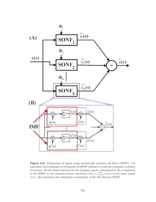
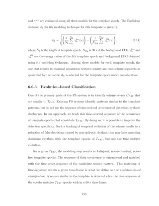
![Figure 6.7 illustrates this novel evolution-based classification approach employed in
the proposed model-based PS system. The modeling process resulted in two disjoint
non-redundant epochs for the given TPAT . The two template epochs of TPAT are
labeled E1and E2 and shown in Fig. 6.7A. Enumerated subscripts denote the time-
order in which they occur in TPAT . The power spectral density plot confirms the
non-overlapping dominant rhythm of the template epochs (Fig. 6.7B). The model-
based PS system for this TPAT consists of two parallel branches of SONF, one for each
template epoch. The detection thresholds are set using the model and the training
data, as described in the classifier training section (Section 6.6.1). The trained PS
system is utilized to detect candidate seizure patterns similar to TPAT . An example of
detected CPAT similar to TPAT is shown in Fig. 6.7C. Raw EEG is shown to map the
detection by the evolution-based classifier. The energy ratios (γ1, γ2) are shown in Fig.
6.7D. The time-sequence of the detected epochs in CPAT is matched to the template
epochs of TPAT to make final detection. In this example, the sequential detection of
template epoch 1 followed by template epoch 2 matches the sequence of the template
epochs in TPAT . The final detection decision is represented by vertical ’dashed’ line in
Fig. 6.7. In this example, there are two instances where the time-ordered template
epochs match. Therefore, there are two detections as indicated by the two dashed
vertical lines.
6.7 Performance Evaluation
The performance of the proposed model-based seizure detection system is assessed on
the MNI database. The MNI database consists of intracranial EEG recordings from
14 patients that was originally scored based on all channels for another study [32]. We
selected the most prominent seizure channel from the multichannel EEG of individual
patients for evaluating the performance of the proposed system, as was done for the
154](https://image.slidesharecdn.com/039fdf0d-408b-485a-969c-4c8bab29d255-160116041507/85/RY_PhD_Thesis_2012-183-320.jpg)
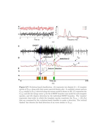
![NPS systems in Chapter 4. For each patient, the first occurring seizure is used as
the template seizure pattern (TPAT ) for the training of the proposed PS system. The
training data includes 30 s of EEG preceding the seizure template. The trained PS
system is used to detect all other seizures that are similar to the template seizure for
the given patient. Same template seizure pattern is used to train the Qu-Gotman
system which, in addition, requires a minimum of 30 minutes of non-seizure EEG.
We selected 30 min section of non-seizure EEG preceding the template pattern. The
background EEG in some patients included one or two patient-disconnection artifacts.
The background EEG is visually inspected for such artifacts. When the background
EEG contains these artifacts, additional seizure-free EEG data is added to compensate
the disconnection artifacts. In all 14 patients, we did not find any manually scored
seizures within the 30 min seizure-free section preceding TPAT for the Qu-Gotman
system. For both the methods, the training data consisted of the first seizure in each
patient (14 template seizures) and the test data included the remaining 4 sections
of data for each patient consisting of a total of 68 seizures in the 304 hours of single
channel EEG for the 14 patients. We used hold-out validation technique in evaluating
the performance of the proposed and Qu-Gotman systems. The test data for each
patient included all EEG sections except the training sections. That is, the test and
training data are mutually exclusive or do not overlap.
A good detection in the proposed system is an event that is detected within 60 s of
the manually scored seizure onset. Prior to performance evaluation, detections within
30 s of one another were grouped as a single detection. We evaluate the Qu-Gotman
system [21] using the same dataset and the same criterion. The performance is assessed
by the three popular measures in the seizure detection literature: sensitivity, specificity,
and false detection rate (FDR), described in Chapter 3.
156](https://image.slidesharecdn.com/039fdf0d-408b-485a-969c-4c8bab29d255-160116041507/85/RY_PhD_Thesis_2012-185-320.jpg)
![6.8 Results
Results of the proposed PS system and the Qu-Gotman system for the individual
patients on the test data are shown in Table 6.1. The model-based PS system resulted
in an overall 100% specificity (FDR = 0/h) and 92.2% sensitivity. Qu-Gotman system
resulted in an overall specificity of 66.6%, sensitivity of 93.7% and a FDR of 0.2/h.
The new PS system reflects a significant improvement (approximately by 33%) in the
specificity when compared to the Qu-Gotman system, but at the cost of a 2% drop in
the sensitivity.
6.9 Discussion
The main goal of the patient-specific seizure detection system in the EMU is to identify
reproducible phenomena that characterize epileptic seizures. The advantage of a PS
system is that it improves the detection sensitivity and reduces the false detection rate.
The proposed model-based PS system significantly improves the detection specificity
resulting in no false detection, while the Qu-Gotman system resulted in a FDR of
0.2/h on the same dataset. Clearly, our method outperforms the popular Qu-Gotman
system.
Although the existing patient-specific seizure detectors show improved sensitivity
and FDR over the generic methods, they are not practical. The main limiting factors
are (a) selection of the template seizure pattern, (b) selection of the background EEG,
and (c) supervised training of the classifier. We have overcome these challenges by
using a novel model-based scheme with SONFs as the building blocks, which can
rapidly track narrowband signals buried in noise [195, 197]. Adaptive modeling and
unsupervised classifier training are some of the key attributes of this new system.
Unlike the multiresolution-based detectors, our PS system is not limited by the
sampling rate. Additionally, seizures with minimal change in the EEG amplitude are
157](https://image.slidesharecdn.com/039fdf0d-408b-485a-969c-4c8bab29d255-160116041507/85/RY_PhD_Thesis_2012-186-320.jpg)
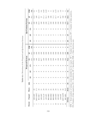
![reported to be generally very difficult to detect by experts as well automatic seizure
detectors. The proposed PS system is capable of detecting low-amplitude seizures,
since it estimates the seizure signals while suppressing the non-seizure EEG, thereby
enhancing the discrimination boundary between the two categories. We have studied
the ability of the proposed system to detect low amplitude seizures using simulated
data1
in [134].
The new PS system resulted in no false detections while missing five out of nine
seizures in Patient 3, one out of three seizures in Patient 4 and one out of five seizures
in Patient 10. An example of the missed seizure and the corresponding template
pattern for Patient 3 (channel: RC1-RC3) is shown in Fig. 6.8. The initial few seconds
of the template pattern contain the mixed frequency characteristics (4 to 34 s) that
later evolve into rhythmic activity. The missed seizure is similar to the mixed seizure
part of the template seizure in the initial seconds (6 to 20 s), but did not continue to
evolve into the rhythmic part. On careful examination of the four derived template
epochs for this patient data, it is observed that the first template epoch corresponded
to the mixed frequency part, while the other three template epochs came from the
rhythmic part of the template pattern (TPAT ). The proposed system is designed to
detect seizures when the candidate seizures match the time-ordered occurrence of the
template epochs in the TPAT . All of the missed seizures in this patient did not meet
this criterion. Clearly, the missed seizure do not match the template seizure.
1
Simulated EEG under varying SNR conditions and durations were used in the development of
the model-based PS system. These are not presented in this thesis.
159](https://image.slidesharecdn.com/039fdf0d-408b-485a-969c-4c8bab29d255-160116041507/85/RY_PhD_Thesis_2012-188-320.jpg)
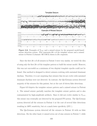
![our system detected all of them with no FDs. The likely cause for the Qu-Gotman
system to miss some of them is the very low EEG amplitude. Additionally, the seizures
missed by the Qu-Gotman system did not evolve in a way similar to the multichannel
template seizure within first 20 s. Seizures can go undetected in the Qu-Gotman
system due to spatial constraints, which require the seizure onsets to occur in the
same channel as those of the template seizure [21]. An example of a training seizure
and a missed seizure in the Qu-Gotman system is shown in Fig. 6.10. Clearly, in this
example, the test seizure in channels other than RH1-RH3 were of low amplitude and
did not evolve in the same manner as the template seizure. No such spatial constraints
exists in our PS system.
Majority of the false detections made by the Qu-Gotman system were brief rhythmic
bursts (< 4-6 s). These short rhythmic discharges did not evolve like the template
seizure pattern, and hence were not detected by our system, resulting in a significantly
improved detection specificity2
.
As with other systems, our system too has limitations. It cannot detect mixed
frequency seizures. The system requires a minimum of two template epochs in order
to make a detection.
Isolating precisely reproducible phenomena in EEG signals remains a difficult task
and is vitally important to answer several fundamental questions and can highlight
possible pathways of the propagation of epileptic discharges. The proposed evolution-
based classification in the PS system allows the identification of recurring seizure
patterns that can accurately map the propagation of epileptic discharges by incorpor-
ating multichannel information; this warrants further research and is considered as
part of future work.
2
It must be noted that Qu-Gotman system is designed as a seizure warning system which requires
the method to have a short detection delay. Our system, while improving the detection specificity,
cannot be used as a seizure warning system because of the constraints imposed in the evolution-based
classification which increases the detection delay.
161](https://image.slidesharecdn.com/039fdf0d-408b-485a-969c-4c8bab29d255-160116041507/85/RY_PhD_Thesis_2012-190-320.jpg)
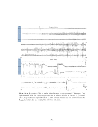


![Chapter 7
Unsupervised Spike Sorting
7.1 Introduction
In epilepsy, little is known as to how normal brain regions become and remain epileptic.
Regardless of the original brain insult, the neocortical epileptic foci show remarkably
similar electrophysiological patterns of localized abnormal electrical discharges. These
discharges become rhythmic and spread to widespread brain regions to produce clinical
seizures. A lot more frequently than seizures, the focal brain regions generate localized
’interictal’ discharges that can be used to identify regions of seizure onset [49, 50, 201].
Interictal discharges commonly known as interictal spikes (ISs) are expressed by high-
amplitude (> 50µV), fast transients often followed by a slow wave for several hundreds
of milliseconds. The hallmark property of interictal spikes are the increased tendency
to recur periodically and often cluster in brief paroxysms [49, 202]. Because normal
neuronal activity is a critical force that shapes nervous system development and
plasticity, it appears that ongoing ictal and interictal epileptic activities influence the
functional and structural changes that lead to hyper-excitability and hyper-connectivity.
Consistent with this idea, gene encodings, neurotransmitter receptors, ion channels,
transcription and neurotrophic factors have been found to be differentially expressed in
165](https://image.slidesharecdn.com/039fdf0d-408b-485a-969c-4c8bab29d255-160116041507/85/RY_PhD_Thesis_2012-194-320.jpg)
![various animal models of epilepsy and in the human epileptic brain tissues [49, 50, 201].
Therefore, it is possible to elucidate activity-dependent molecular pathways linked
with epilepsy. This can be achieved by comparing “electrically-active neocortex” to
“control neocortex” within the same patient to search for common gene expression
changes across many patients [49, 50, 201]. Furthermore, even though as to how
exactly interictal spikes develop, propagate and contribute to the generation of seizures
is not well understood, several studies report a better surgical outcome when regions
of frequent interictal spikes are also removed [45, 203]. Qualitative and quantitative
analysis of interictal spikes thus become vitally important for epilepsy management.
However, no such tool exists for use with intracranial EEG recordings.
In this chapter, we propose a new unsupervised spike sorting method to facilitate
rapid qualitative and quantitative analysis of interictal spikes for intracranial EEG
[204, 205]. The performance of the proposed sorting method is compared against a
popular unsupervised spike sorting technique (WAVE CLUS1
) [151] that is designed
for extracellular potentials.
Keeping in mind the heavy workload of the clinical staff in the EMUs, we unify the
proposed spike sorting algorithm with a simple, easy-to-use graphical user interface
(GUI). Hereafter, we will refer to complete spike classification software package as the
automatic spike classification (ASC) package.
7.2 Challenges in Spike Sorting
Spike sorting is the first step in the qualitative and quantitative analysis of neural spikes.
The process involves detecting spikes and clustering or mapping each spike to its source.
It is generally considered a high dimensional clustering problem that still remains
incompletely-solved due to issues of signal-to-noise ratio (SNR), non-stationarity, and
1
Wave Clus spike sorting system is designed for sorting action potentials and not for the interictal
spikes.
166](https://image.slidesharecdn.com/039fdf0d-408b-485a-969c-4c8bab29d255-160116041507/85/RY_PhD_Thesis_2012-195-320.jpg)
![non-Gaussianity. Artifacts resembling spikes lead to erroneous classification [147, 153,
154, 206-210]. The two major challenges to be faced in the analysis of interictal spikes,
are the wide variety of spike morphologies and the lack of a priori knowledge of spike
information for each patient. Manual correction of the sorting errors and the sorting
results thus become mandatory; this is time-intensive and subjective [211].
A large number of electrodes introduces computational complexity that can vary
from patient to patient. Furthermore, EEG is digitized at different sampling rates (200
to 5000 Hz) across various laboratories. Sorting methods based on multi-resolution
analysis, such as the wavelet transform, are dependent on the sampling rate, which
ultimately limits their widespread application [155, 209]. Majority of the spike sorting
algorithms in the literature parametrize spikes into a high dimensional feature space to
overcome the data sparsity and low SNR. However, representation of spikes in terms
of features loses the morphology of the spikes, which can be important in the invasive
studies [155, 209].
Validation of the spike sorting results is another challenge, since spike classes
are not known a priori. Typically, the sorting results are evaluated using one or
more cluster validity metrics on simulated data for varying SNR and with a limited
number of spike classes. The popular performance evaluation measures are intra- and
inter- cluster distance, Folkes and Mallows index, Huberts Γ statistics, cophenetic
correlation coefficient, Dunn index, Davies-Bouldin index, and Xie-Beni index [212].
These measures give an indication of the cluster quality, which requires experts to
visually screen the spikes and validate the automatic sorting results.
In this chapter, we propose a new spike sorting method, designed for prolonged
depth EEG recordings, that address some of the above practical issues. This chapter
also proposes an easy-to-interpret cluster validation method.
167](https://image.slidesharecdn.com/039fdf0d-408b-485a-969c-4c8bab29d255-160116041507/85/RY_PhD_Thesis_2012-196-320.jpg)
![7.3 Automatic Spike Classification
In the literature, it has been reported that template matching sorting methods
outperform other sorting techniques. These methods, however, require complete
knowledge of the data, and often employ principal component analysis (PCA) and
wavelet transformations to generate the templates [209, 213]. Taking into account
the superior performance of the template matching sorting techniques, we propose
a sorting algorithm that uses template matching at its core, but does not require a
priori knowledge of all the data to generate the templates. That is, the templates
are created on-the-fly as the data becomes available. Thus, one of the primary goals
in the proposed method is to generate the best representation of the template, as
the clustering outcomes are heavily dependent on the templates. Since spike wave
complexes are crucial in epilepsy research, we propose a full waveform-based sorting
algorithm. Challenges in waveform-based sorting techniques mainly arise due to
noise, data dimensionality and sparsity. In multichannel recordings, adjacent channels
sometimes contain the same type of spike activity. In these cases, correlations between
channels can be exploited to generate templates for which we consider a morphological
correlator and the PCA. Waveform-based sorting methods suffer from transient and
unavoidable gradual changes in the spike waveform (waveform nonstationarities),
resulting in the creation of a large number of overlapping clusters. To eliminate
this type of sorting errors, we employ an offline method (hierarchical clustering and
validation) that uses a priori knowledge of the templates and the spike waveforms
to improve the quality of the sorting results. The proposed sorting algorithm is
shown in the block diagram enclosed by thick ’blue’ rectangular box in Fig. 7.1 and
is composed of five blocks: (a) spike alignment, (b) morphological correlator, (c)
principal component analysis, (d) template matching, and (e) hierarchical clustering
and validation.
It is important to define the various terms used in the proposed method before
168](https://image.slidesharecdn.com/039fdf0d-408b-485a-969c-4c8bab29d255-160116041507/85/RY_PhD_Thesis_2012-197-320.jpg)
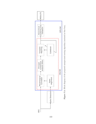
![describing each of the building blocks. We define a single channel detected spike
as the reference spike irrespective of whether the spike was detected automatically
or manually. Multichannel EEG centered around the vertex of the reference spike
is defined as the multichannel spike event. Let X = [x1, x2, ..., xN ] represent the
multichannel spike event, where N is the number of channels and the column xi
represents the ith channel spike data of length n. A variety of clinical studies examine
not only the spike, but also the waveform following the spike which we define as the
spike-wave-complex (SWC). Therefore, 150 ms of the EEG following the spike event
is added to create the SWC. Let Y = [yi, y2, ...yN ] represent the N-channel SWCs,
where each column is a vector of length m. In our analysis, m = 250 ms (± 50 ms
of spike data around the spike vertex and 150 ms of data following the spike event)
was empirically found to be optimal in this development. Since the proposed method
generates templates on-the-fly by exploiting the spatial correlation between adjacent
channels, aligning spikes to a common reference point (which is the vertex of reference
spike) becomes inevitable and is the first step in the proposed method. Both X and Y
represent aligned multichannel spike data. Figure 7.2 illustrates the multichannel EEG
extracted around the reference spike, aligned multichannel spike and the resulting
SWC event. A template is defined as the optimal or best single-channel representation
for a group (class) of similar SWC events and a codebook is defined as a collection of
SWC templates for a patient.
7.3.1 Spike Data (Spike Detection)
The state-dependent spike detection algorithm of [159] available in the Stellate Har-
monie v6.2e software (Stellate Inc, Montreal, Canada) is employed to identify spikes,
which we refer to as the AutoSpike events. Same patient data is also scored for spike
events by an experienced EEGer. Manually identified spikes will be referred to as
the ManuSpike events. Even though previously detected spikes are utilized for spike
170](https://image.slidesharecdn.com/039fdf0d-408b-485a-969c-4c8bab29d255-160116041507/85/RY_PhD_Thesis_2012-199-320.jpg)

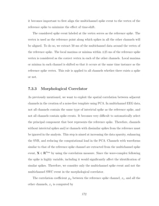
![ρij =
nΣxixj − (Σxi)(Σxj)
n(Σx2
i ) − (Σxi)2 n(Σx2
j ) − (Σxj)2
, (7.1)
where n is the length of the spikes. The correlation coefficient ρij between the ith
reference spike and jth channel is compared to a threshold, ρMC. If ρij exceeds ρMC,
then channels with spikes similar to the reference spike are identified. In this manner,
only those channels similar to the reference spike channel are retained for further
analysis, as shown in Fig. 7.3. This step reduces the data dimension and is similar
to subtractive clustering technique in [213]. In subtractive clustering, similar spikes
around the defined cluster center point (reference spike) are searched and extracted,
and the process iterates until all of the data belongs to unique classes.
Figure 7.3: Identification of channels with spikes similar to the reference spike using
morphological correlator.
7.3.4 Principal Component Analysis
The output of the morphological correlator along with the wave-complexes following
the spike represents the multichannel SWC event, Y. We apply PCA to the resulting
multichannel SWC event to generate a noise-free estimate of the template spike. PCA
173](https://image.slidesharecdn.com/039fdf0d-408b-485a-969c-4c8bab29d255-160116041507/85/RY_PhD_Thesis_2012-202-320.jpg)
![is a linear mathematical transform that seeks a projection of the correlated data to a
new uncorrelated coordinate system called principal components. These coordinates
are an ordered set of orthogonal basis vectors that capture the directions of the largest
variation in the data. It has been shown that incorrectly aligned spike waveforms
affect the projection bases in the PCA and thus, the clustering outcome [214, 215]. It
is for this reason that we align the spike vertex across channels.
For the implementation of PCA, the mean-centered signals, Yc are whitened using
the following equation:
Z = V · Yc, (7.2)
where V = Λ−1/2
UT
is the whitening matrix, Λ = diag[λ1, ..., λk] and U are the
eigenvalue and eigenvector matrices, respectively, of the covariance matrix of YC.
Mean centering is necessary for performing PCA to ensure that the first principal
component describes the direction of maximum variance. In Eq. (7.2), each column zi
corresponds to the projection of y on the ith
principal component ui, and the variance
of the component zi is λi such that λ1 > λ2 >, ..., > λk.
In high SNR conditions, the first principal component (highest variance) corres-
ponds to the signal (reference SWC) while low variance components correspond to
noise. In low SNR conditions, the selection of principal components corresponding
to the SWC event becomes more complex. In the framework of unsupervised spike
sorting, we want to automatically select the component that best represents the SWC.
By employing the morphological correlator as a preprocessing step, we eliminate
channels that do not contain information related to the reference spike. This results
in a high SNR condition, where the best representation of the reference SWC is the
first principal component. Therefore, the first principal component is considered as
the candidate SWC, wi, as shown in Fig. 7.4.
174](https://image.slidesharecdn.com/039fdf0d-408b-485a-969c-4c8bab29d255-160116041507/85/RY_PhD_Thesis_2012-203-320.jpg)
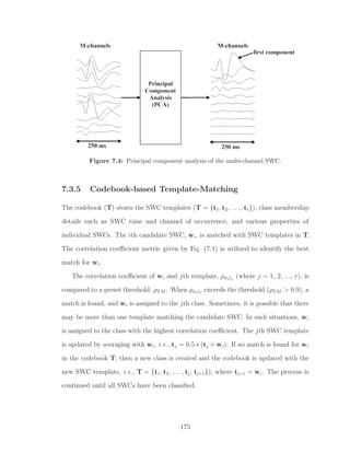
![7.3.6 Hierarchical Clustering and Post-classification
Since the SWC templates evolve over time, they are highly susceptible to noise and
EEG non-stationarity, resulting in the creation of redundant classes. Furthermore,
since interictal spike-wave-complexes tend to recur periodically, a large number of
these events will be concentrated in clusters with large number of members. Therefore,
sorting results can be further improved by identifying and rejecting overlapping and
insignificant clusters.
Kaneko et al. [153] utilized the bottom-up approach (agglomerative) hierarchical
clustering to identify and merge similar classes. We too employ agglomerative clustering
using single linkage rule, where the similarity parameter is the Mahalanobis distance
to identify and merge similar classes. In this approach, the process iterates until all
objects are aggregated into a single class using the distance measure. The distance,
di,j, between ith and jth class is evaluated using the Mahalanobis distance given by
di,j = µi − µj
T
Σ−1 µi − µj (7.3)
where µ and are the SWC classes and the covariance matrix, respectively. The
threshold to merge clusters based on the Mahalanobis distance between cluster centers
is set to 0.1 and is adapted from [216]. This results in well-separated clusters.
In our application, we are only interested in clusters with a significantly large
number of members. Since rarely occurring SWC events and events due to noise and
artifacts are expected to have a relatively low number of members in the clusters. By
applying a threshold relative to the highest-ranking cluster (cluster with the highest
number of members), we can reject clusters that contain rarely occurring events and
events due to noise and artifacts, thus improving the codebook quality. Therefore, we
examined the number of spikes lost with this relative threshold on the five patients
training data. Figure 7.5 illustrates the effect of the relative threshold on the number
176](https://image.slidesharecdn.com/039fdf0d-408b-485a-969c-4c8bab29d255-160116041507/85/RY_PhD_Thesis_2012-205-320.jpg)
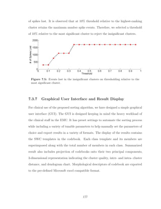
![7.4 Performance Evaluation
A popular unsupervised spike sorting technique ’WAVE CLUS’ [151] for extracellular
recordings is considered for comparison. The inputs to the WAVE CLUS are AutoSpike
and ManuSpike events. The sorting results are visually assessed for the number of
overlapping clusters in the codebook.
One of the main challenges in the spike sorting is the lack of a priori knowledge
of the total number of classes or clusters in the data. Researchers, therefore, often
validate their spike sorting methods using simulated data with a fixed number of
spike classes [155, 207]. On real data, algorithm performance may vary and requires
mandatory visual inspection of the sorting results. Evaluating the clustering results
by traditional approaches is time-consuming and highly subjective.
We propose a new indirect approach to validate our sorting method, which estab-
lishes a definite role for automatic spike detection and sorting methods for clinical
application. In this approach, we compare the sorting results of spike events detected
by two different approaches - automatic spike detector (AutoSpike) and the gold
standard manual spike scoring by the EEGer (ManuSpike). Codebooks generated
using the two sets of spike data for the same patient are expected to have the same
number and type of classes. Therefore, the spike sorting method can be indirectly
validated by visually comparing the codebooks for the two sets of spikes. We refer to
these two codebooks as the AutoSpike- and Manuspike-codebooks for each patient. To
facilitate easy visual assessment of the sorting result, we employ visual cluster analysis
techniques.
Visualization mitigates the challenges in traditional approaches of cluster validation.
It maps the high-dimensional data to a 2D or 3D space and aids users having an intuitive
and easily understood graph/image to reveal the grouping relationship between the
data [217, 218]. Several techniques have been proposed for visual cluster analysis
such as icon-based, pixel-oriented, and geometric techniques, and multidimensional
178](https://image.slidesharecdn.com/039fdf0d-408b-485a-969c-4c8bab29d255-160116041507/85/RY_PhD_Thesis_2012-207-320.jpg)
![scaling maps such as hierarchical blob, self-organizing maps, and PCA [217, 218].
However, visual assessment of quality of clustering result still heavily relies on the
user’s visual perception and understanding on cluster distribution. We include two
different easy-to-interpret cluster visualizations: (a) geometric technique, and (b)
dendogram.
7.4.1 Geometric Technique
The basic idea of geometric technique is to visualize transformations and projections
of the data to produce useful and insightful visualizations. We propose a new easy-
to-interpret visual cluster analysis technique, which is a combination of visualization
and cluster analysis. We represent the cluster quality metrics in 3D space as spheres.
The center of the sphere is the centroid of the cluster and radius of the sphere is
the variation within the cluster (intra-cluster distance). The centroid of a cluster
is the average of all SWC points for the given cluster. Since waveform variations
in a cluster can lead to shift in the actual cluster center, we compute the cluster
centroid using the first principal component from PCA instead of directly deriving
it from the cluster. The ith cluster is represented as sphere Si at center Pi of radius
ri = σ2
i , where Pi = {ci, ci, ci} and ci is the centroid of the first principal component
of the ith cluster in the codebook. The inter-cluster distance is the Mahalanobis
distance between the ith and jth cluster. The resulting 3D visualization allows an easy
identification of overlapping clusters, where disjoint spheres symbolize non-overlapping
clusters. The example in Fig. 7.6 shows the 3D representation of the inter- and intra-
cluster distances obtained using the AutoSpike events of a patient before applying
the hierarchical clustering. At this stage, the codebook contains six clusters of which
two are well separated and compact (A and B), while two pairs of clusters overlap (C,
D) and (E, F). It is noted that in the pair (E, F), one of the overlapping clusters (F)
appears to be much less compact than the other (E), i.e., larger intra-cluster distance.
179](https://image.slidesharecdn.com/039fdf0d-408b-485a-969c-4c8bab29d255-160116041507/85/RY_PhD_Thesis_2012-208-320.jpg)


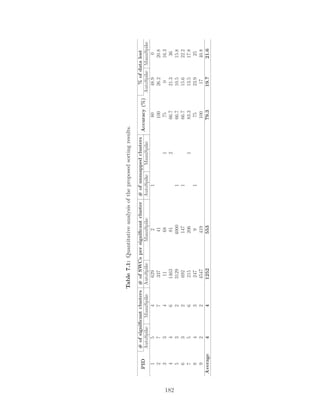
![accuracy is not reported for the WAVE CLUS algorithm.
7.6 Discussion
The purpose of this study was to develop an unsupervised sorting technique to aid in
the rapid quantitative analysis of interictal spikes and establish definite role of spike
detection and sorting techniques for clinical application in the EMU.
Template matching-based sorting methods are the most preferred technique in the
literature because of their superior performance. These methods, however, require a
knowledge of the complete data to derive the templates. Therefore, template-matching
sorting methods are generally not well suited for online analysis. We have proposed a
novel online spike sorting technique that employs template-matching at its core and
dynamically derives the templates as the data becomes available.
Majority of the spike sorting methods in the literature extract various features
of spikes such as spike height, width, peak-to-peak amplitude, half-wave duration,
slopes, and wavelet coefficients. These features are utilized to measure similarity
between spikes to perform sorting. Classifying spikes directly using waveforms in
high dimensional space is considered very challenging because data points are sparse
and noisy, resulting in imprecise clusters [147, 211, 219]. Waveform morphology is
vitally important in invasive EEG studies. Therefore, representation of the spike wave
complex into features is not generally suitable. To address this clinical need, we have
proposed a multistage complete waveform-based sorting technique.
We have incorporated PCA to generate the noise-free estimate of the templates.
However, PCA requires a set of synchronized spikes to perform PCA. We have used
the reference spike (defined earlier) to align data on other channels prior to processing
the multichannel SWC by PCA to generate the best estimate for the SWC candidate.
When multichannel SWC events are not available for PCA, the SWC event is considered
183](https://image.slidesharecdn.com/039fdf0d-408b-485a-969c-4c8bab29d255-160116041507/85/RY_PhD_Thesis_2012-212-320.jpg)
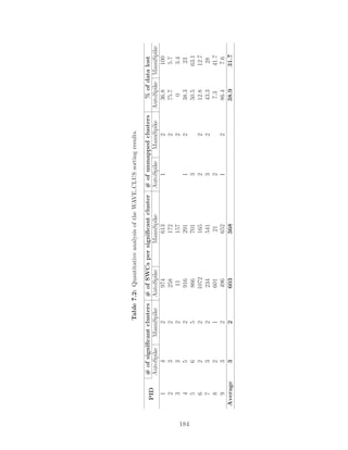
![as the SWC candidate.
In the literature, there exist a few template-matching sorting techniques that dy-
namically derive templates, but such methods have been shown to result in overlapping
clusters [206, 220-222]. Visual assessment of sorting results, therefore, becomes very
difficult. The challenges arise due to (1) overlapping clusters, and (2) unknown number
of clusters. The latter is application dependent and does not have a general solution.
However, the issue of overlapping clusters that arises due to noise and artifacts can be
resolved. It has been shown in [153] that tracking spike-amplitude changes improves
the quality of the spike templates and reduces the number of overlapping clusters. We
have also followed a similar approach to minimize the influence of noise and artifacts.
The templates are continually updated over time whenever a matching event is found.
This is advantageous as it improves the SNR of the SWC template and results in a
reduction of number of overlapping clusters.
Kaneko et al. [153] showed that tracking spike clusters by repeatedly applying
bottom-up hierarchical clustering to spike data recorded during temporally overlapping
frames helps in improving the quality of the sorting results. However, repeatedly
applying hierarchical clustering is computationally expensive. Instead of repeatedly
performing hierarchical clustering on each subsequent frame, the same can be applied
on the codebook once the online analysis has been completed. Our method identifies
and merges overlapping clusters in the codebook using hierarchical clustering once the
online analysis has been completed. This improves the quality of the sorting results.
The codebook contains clusters that are due to interictal spikes as well as rarely
occurring events and artifacts. The EEGer is mainly interested in the significant
clusters. This is because significant clusters are likely to contain the highly stereotypical
recurring interictal spikes. Therefore, clusters with lower membership can be deleted
from the codebook. We reject clusters with number of SWC members below some
percentage of the most significant cluster membership. This improves the quality of
185](https://image.slidesharecdn.com/039fdf0d-408b-485a-969c-4c8bab29d255-160116041507/85/RY_PhD_Thesis_2012-214-320.jpg)
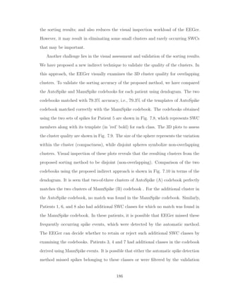
![Figure 7.8: Codebook generated using AutoSpike and ManuSpike events for Patient 5
using the proposed spike sorting algorithm.
block (due to lower cluster membership). The cut-off threshold in the validation block
is a function of the class with the highest membership. Therefore, some of the SWC
classes with lower membership may have been rejected. It is important to mention
that the EEGer may not have access to both the AutoSpike and Manuspike codebooks.
The two codebooks were employed to validate the sorting results in the absence of
true class labels. Validation of the sorting results with this indirect approach reported
good matching between the two codebooks. This establishes a definite role for spike
detection and the proposed sorting method for clinical use. The EEGer can rapidly
examine the codebook, thereby significantly reducing the cost of identifying and
classifying events by the experts.
We have also compared our sorting method with a popular spike sorting tech-
nique WAVE CLUS [151]. The AutoSpike and ManuSpike events were input to the
WAVE CLUS sorting algorithm to generate the two codebooks. Sorting was performed
at the default settings of the algorithm and summary of the sorting results are shown
in Table 7.2. The sorting results for Patients 4 and 9 obtained using the AutoSpike
events by the proposed and WAVE CLUS techniques, respectively, are shown in Fig.
187](https://image.slidesharecdn.com/039fdf0d-408b-485a-969c-4c8bab29d255-160116041507/85/RY_PhD_Thesis_2012-216-320.jpg)
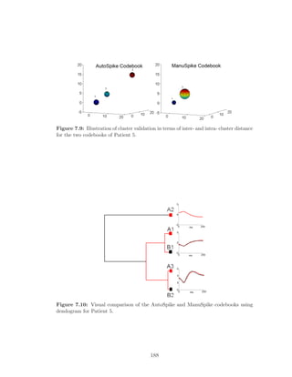
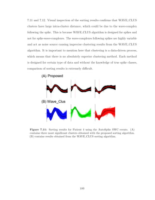
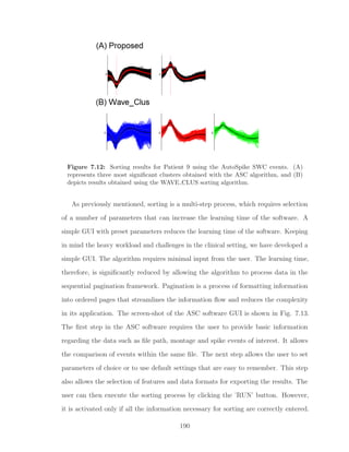
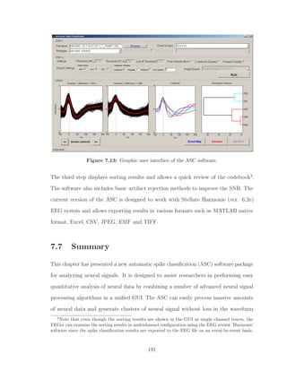
![(HFOs). HFOs are low-amplitude transient events that are thought to play a
role in the physiological and pathological neural process [223-227]. We have
demonstrated that the new sharpness of EEG waveform feature is highly sensitive
to changes in the amplitude and frequency. We believe that this feature can be
utilized to make computationally light and robust HFO detector.
• The ideal spike detector does not exist as the specificity and sensitivity remain
difficult to assess when there exists a large variability in the visual classification
by the experts [228]. Nonetheless, the waveform sharpness is one of the most
important characteristics of an interictal spike, which can be explored with
respect to the new feature proposed in this thesis to develop a reliable spike
detector.
• It has been noted that the detection specificity of the new NPS system proposed
in this thesis may deteriorate in the presence of sharp transients, high-frequency
electromyographic activity and high-amplitude artifacts. New artifact rejection
strategies need to be explored to handle such artifacts. Since scalp EEG is prone
to additional artifacts, extending the new NPS systems to scalp EEG would
require additional considerations.
• The RSI display allows rapid identification of epileptogenic sites. However, the
new compressed EEG display does not provide any quantitative information of
the epileptiform activity. Information such as seizure recurrence, onset zone, and
spreads, are manually identified by the expert. Manual identification of these
crucial informations is extremely tiresome and subjective. These informations
can be made available by combining the RSI display, NPS and the PS systems
developed in this thesis, which could improve the care and management of
epilepsy patients, and therefore, must be investigated.
200](https://image.slidesharecdn.com/039fdf0d-408b-485a-969c-4c8bab29d255-160116041507/85/RY_PhD_Thesis_2012-229-320.jpg)

![artifacts must be removed to ensure that components representing EEG activity
are preserved [229]. Therefore, extending the new PS system to scalp EEG
would require additional considerations to handle these artifacts.
8.3.3 Spike Sorting System
The proposed spike sorting system provides the basic tool necessary for the analysis
of interictal spikes. The method can be improved on several fronts, and some of the
possible avenues are listed below.
• Alignment of the spikes to its maximum amplitude plays a pivotal role in the
success of the proposed method. However, local maximum of the spike may
get corrupted by the noise causing misalignment. Smoothing techniques such
as cubic spline interpolation can be explored to minimize the effect of noise.
Aligning spikes to the point of its maximum slope or frequency-weighted energy
can also be explored; these should further improve the classification results.
• Aligning spikes in the multichannel EEG distorts the spike propagation pathways,
which are vitally important in some clinical studies such as epilepsy. Instead of
aligning multichannel EEG with the reference spike, the multichannel spike event
can be used directly as a template. This will result in multichannel templates
instead of a single-channel template and will preserve the spike propagation
pathways. However, this will lead to templates with poor SNR that can result
in an increased number of misclassification and overlapping clusters. Effect of
noise in the multichannel template can be minimized by exploring techniques
such as independent component analysis (ICA). The benefits of ICA are many,
including the ability to automatically detect artifacts and overlapping spikes
and to handle waveform non-stationarities [230]. However, it must be noted that
the ICA, an iterative algorithm, is computationally expensive.
202](https://image.slidesharecdn.com/039fdf0d-408b-485a-969c-4c8bab29d255-160116041507/85/RY_PhD_Thesis_2012-231-320.jpg)
![An obvious extension of the proposed sorting method would be in the statistical
characterization of the spatio-temporal distribution of interictal spikes in a large
dataset and identifying the subsets of brain structures frequently and conjointly
involved in the generation of interictal spikes [228].
203](https://image.slidesharecdn.com/039fdf0d-408b-485a-969c-4c8bab29d255-160116041507/85/RY_PhD_Thesis_2012-232-320.jpg)
![References
[1] World Health Organization, ATLAS : Epilepsy care in the world. World Health
Organization, 2005.
[2] R. S. Fisher, G. Harding, G. Erba, G. L. Barkley, and A. Wilkins, “Photic-
and pattern-induced seizures: a review for the epilepsy foundation of america
working group,” Epilepsia, vol. 46, no. 9, pp. 1426–41, 2005.
[3] F. Mormann, R. G. Andrzejak, T. Kreuz, C. Rieke, P. David, C. E. Elger, and
K. Lehnertz, “Automated detection of a preseizure state based on a decrease in
synchronization in intracranial electroencephalogram recordings from epilepsy
patients,” Physical Review E, vol. 67, no. 2 Pt 1, p. 021912, 2003.
[4] I. Kotsopoulos, T. Van Merode, F. Kessels, M. De Krom, and J. Knottnerus,“Sys-
tematic review and meta-analysis of incidence studies of epilepsy and unprovoked
seizures,” Epilepsia, vol. 43, no. 11, pp. 1402–1409, 2002.
[5] E. Niedermeyer and F. L. D. Silva, Electroencephalography: Basic Principles,
Clinical Applications, and Related Fields. Lippincott Williams & Wilkins, 2004.
[6] “ILAE classification of epilepsies: its applicability and practical value of different
diagnostic categories,” Epilepsia, vol. 37, no. 11, pp. 1051–9, 1996.
204](https://image.slidesharecdn.com/039fdf0d-408b-485a-969c-4c8bab29d255-160116041507/85/RY_PhD_Thesis_2012-233-320.jpg)
![[7] D. Schmidt and S. C. Schachter, Puzzling cases of epilepsy. Academic Press,
2008.
[8] C. G. Wasterlain and D. M. Treiman, Status Epilepticus : mechanisms and
management. MIT Press, 2006.
[9] G. Adelman and B. H. Smith, Encyclopedia of Neuroscience. Elsevier, 1999.
[10] X. F. Yang and S. M. Rothman, “Focal cooling rapidly terminates experimental
neocortical seizures,” Annals of Neurology, vol. 49, no. 6, pp. 721–6, 2001.
[11] X. F. Yang, D. W. Duffy, R. E. Morley, and S. M. Rothman, “Neocortical seizure
termination by focal cooling: temperature dependence and automated seizure
detection,” Epilepsia, vol. 43, no. 3, pp. 240–5, 2002.
[12] B. Litt and J. Echauz, “Prediction of epileptic seizures,” Lancet Neurology, vol. 1,
no. 1, pp. 22–30, 2002.
[13] W. S. Anderson, E. H. Kossoff, G. K. Bergey, and G. I. Jallo, “Implantation
of a responsive neurostimulator device in patients with refractory epilepsy,”
Neurosurgical Focus, vol. 25, no. 3, p. E12, 2008.
[14] T. L. Skarpaas and M. J. Morrell, “Intracranial stimulation therapy for epilepsy,”
Neurotherapeutics, vol. 6, no. 2, pp. 238–43, 2009.
[15] S. Wong, G. H. Baltuch, J. L. Jaggi, and S. F. Danish, “Functional localization
and visualization of the subthalamic nucleus from microelectrode recordings
acquired during DBS surgery with unsupervised machine learning,” Journal of
Neural Engineering, vol. 6, no. 2, p. 026006, 2009.
[16] K. B. Baker, B. H. Kopell, D. Malone, C. Horenstein, M. Lowe, M. D. Phillips,
and A. R. Rezai, “Deep brain stimulation for obsessive-compulsive disorder:
using functional magnetic resonance imaging and electrophysiological techniques:
205](https://image.slidesharecdn.com/039fdf0d-408b-485a-969c-4c8bab29d255-160116041507/85/RY_PhD_Thesis_2012-234-320.jpg)
![technical case report,”Neurosurgery, vol. 61, no. 5 Suppl 2, pp. E367–8; discussion
E368, 2007.
[17] S. M. Rothman, “The therapeutic potential of focal cooling for neocortical
epilepsy,” Neurotherapeutics, vol. 6, no. 2, pp. 251–7, 2009.
[18] S. Raghunathan, S. K. Gupta, M. P. Ward, R. M. Worth, K. Roy, and P. P.
Irazoqui, “The design and hardware implementation of a low-power real-time
seizure detection algorithm,” Journal of Neural Engineering, vol. 6, no. 5,
p. 56005, 2009.
[19] H. Qu and J. Gotman, “Improvement in seizure detection performance by
automatic adaptation to the EEG of each patient,” Electroencephalography and
Clinical Neurophysiology, vol. 86, no. 2, pp. 79–87, 1993.
[20] H. Qu, Self-adapting algorithms for seizure detection during EEG monitoring.
PhD thesis, Department of Biomedical Engineering, McGill University, 1994.
[21] H. Qu and J. Gotman, “A patient-specific algorithm for the detection of seizure
onset in long-term EEG monitoring: possible use as a warning device,” IEEE
Transactions on Biomedical Engineering, vol. 44, no. 2, pp. 115–22, 1997.
[22] J. Gotman, “Automatic recognition of interictal spikes,” Electroencephalography
and Clinical Neurophysiology, vol. 37, pp. 93–114, 1985.
[23] D. Zumsteg, D. M. Andrade, and R. A. Wennberg, “Source localization of small
sharp spikes: low resolution electromagnetic tomography (LORETA) reveals two
distinct cortical sources,” Clinical Neurophysiology, vol. 117, no. 6, pp. 1380–7,
2006.
[24] E. Niedermeyer, “The clinical relevance of EEG interpretation,” Clinical Electro-
encephalography, vol. 34, no. 3, pp. 93–8, 2003.
206](https://image.slidesharecdn.com/039fdf0d-408b-485a-969c-4c8bab29d255-160116041507/85/RY_PhD_Thesis_2012-235-320.jpg)
![[25] E. Niedermeyer, “Ultrafast EEG activities and their significance,” Journal of
Clinical EEG and Neuroscience, vol. 36, no. 4, pp. 257–62, 2005.
[26] T. Yu, Y. Wang, G. Zhang, L. Cai, W. Du, and Y. Li, “Posterior cortex epilepsy:
Diagnostic considerations and surgical outcome,” Seizure, 2009.
[27] M. Zijlmans, J. Jacobs, Y. U. Kahn, R. Zelmann, F. Dubeau, and J. Gotman,
“Ictal and interictal high frequency oscillations in patients with focal epilepsy,”
Clinical Neurophysiology, vol. 122, no. 4, pp. 664–71, 2011.
[28] F. Wendling, J. J. Bellanger, J. M. Badier, and J. L. Coatrieux, “Extraction of
spatio-temporal signatures from depth EEG seizure signals based on objective
matching in warped vectorial observations,” IEEE Transactions on Biomedical
Engineering, vol. 43, no. 10, pp. 990–1000, 1996.
[29] F. Wendling, M. B. Shamsollahi, J. M. Badier, and J. J. Bellanger, “Time-
frequency matching of warped depth-EEG seizure observations,” IEEE Transac-
tions on Biomedical Engineering, vol. 46, no. 5, pp. 601–5, 1999.
[30] R. Meier, H. Dittrich, A. Schulze-Bonhage, and A. Aertsen, “Detecting epileptic
seizures in long-term human EEG: a new approach to automatic online and
real-time detection and classification of polymorphic seizure patterns,” Journal
of Clinical Neurophysiology, vol. 25, no. 3, pp. 119–31, 2008.
[31] J. Gotman, “Automatic detection of seizures and spikes,” Journal of Clinical
Neurophysiology, vol. 16, no. 2, pp. 130–40, 1999.
[32] S. Grewal and J. Gotman, “An automatic warning system for epileptic seizures
recorded on intracerebral EEGs,” Clinical Neurophysiology, vol. 116, no. 10,
pp. 2460–72, 2005.
207](https://image.slidesharecdn.com/039fdf0d-408b-485a-969c-4c8bab29d255-160116041507/85/RY_PhD_Thesis_2012-236-320.jpg)
![[33] R. Yadav, R. Agarwal, and M. N. S. Swamy, “A novel dual-stage classifier for
automatic detection of epileptic seizures,” Proceedings of IEEE Engineering in
Medicine and Biology Society Conference, pp. 911–914, 2008.
[34] R. Yadav, R. Agarwal, and M. N. S. Swamy,“A novel morphology-based classifier
for automatic detection of epileptic seizures,” Proceedings of IEEE Engineering
in Medicine and Biology Society Conference, pp. 5545–5548, 2010.
[35] A. S. Zandi, M. Javidan, G. A. Dumont, and R. Tafreshi, “Automated real-time
epileptic seizure detection in scalp EEG recordings using an algorithm based
on wavelet packet transform,” IEEE Transactions on Biomedical Engineering,
vol. 57, no. 7, pp. 1639–51, 2010.
[36] R. Yadav, R. Agarwal, and M. N. S. Swamy, “Detection of epileptic seizures
in stereo-EEG using frequency-weighted energy,” Proceedings of IEEE Midwest
Symposium on Circuits and Systems, pp. 77–80, 2007.
[37] R. Yadav, R. Agarwal, and M. N. S. Swamy, “STFT-based segmentation in
model-based seizure detection,” Proceedings of IEEE Canadian Conference on
Electrical and Computer Engineering, pp. 729–732, 2007.
[38] C. I. Akman, V. Micic, A. Thompson, and J. J. Riviello, “Seizure detection
using digital trend analysis: Factors affecting utility,” Epilepsy Research, vol. 93,
pp. 66–72, Jan 2011.
[39] R. Agarwal, J. Gotman, D. Flanagan, and B. Rosenblatt, “Automatic EEG
analysis during long-term monitoring in the ICU,” Electroencephalography and
Clinical Neurophysiology, vol. 107, pp. 44–58, Jul 1998.
[40] A. K. Shah, R. Agarwal, J. R. Carhuapoma, and J. A. Loeb, “Compressed EEG
pattern analysis for critically ill neurological-neurosurgical patients,” Neurocrit-
ical Care, vol. 5, no. 2, pp. 124–33, 2006.
208](https://image.slidesharecdn.com/039fdf0d-408b-485a-969c-4c8bab29d255-160116041507/85/RY_PhD_Thesis_2012-237-320.jpg)
![[41] C. P. Stewart, H. Otsubo, A. Ochi, R. Sharma, J. S. Hutchison, and C. D. Hahn,
“Seizure identification in the ICU using quantitative EEG displays,” Neurology,
vol. 75, no. 17, pp. 1501–8, 2010.
[42] V. Gnatkovsky, S. Francione, F. Cardinale, R. Mai, L. Tassi, G. L. Russo, and
M. de Curtis, “Identification of reproducible ictal patterns based on quantified
frequency analysis of intracranial EEG signals.,” Epilepsia, vol. 52, pp. 477–488,
Mar 2011.
[43] R. Wagner, D. M. Feeney, F. P. Gullotta, and I. L. Cote, “Suppression of cortical
epileptiform activity by generalized and localized ECoG desynchronization,”
Electroencephalography and Clinical Neurophysiology, vol. 39, no. 5, pp. 499–506,
1975.
[44] T. E. Peters, N. C. Bhavaraju, M. G. Frei, and I. Osorio, “Network system for
automated seizure detection and contingent delivery of therapy,” Journal of
Clinical Neurophysiology, vol. 18, no. 6, pp. 545–9, 2001.
[45] E. D. Marsh, B. Peltzer, r. Brown, M. W., C. Wusthoff, J. Storm, P. B., B. Litt,
and B. E. Porter, “Interictal EEG spikes identify the region of electrographic
seizure onset in some, but not all, pediatric epilepsy patients,” Epilepsia, vol. 51,
no. 4, pp. 592–601, 2010.
[46] R. G. Emerson, C. A. Turner, T. A. Pedley, T. S. Walczak, and M. Forgione,
“Propagation patterns of temporal spikes,” Electroencephalography and Clinical
Neurophysiology, vol. 94, no. 5, pp. 338–48, 1995.
[47] E. Asano, O. Muzik, A. Shah, C. Juhasz, D. C. Chugani, S. Sood, J. Janisse, E. L.
Ergun, J. Ahn-Ewing, C. Shen, J. Gotman, and H. T. Chugani, “Quantitative
interictal subdural EEG analyses in children with neocortical epilepsy,” Epilepsia,
vol. 44, no. 3, pp. 425–34, 2003.
209](https://image.slidesharecdn.com/039fdf0d-408b-485a-969c-4c8bab29d255-160116041507/85/RY_PhD_Thesis_2012-238-320.jpg)
![[48] J. Bourien, F. Bartolomei, J. J. Bellanger, M. Gavaret, P. Chauvel, and F. Wend-
ling, “A method to identify reproducible subsets of co-activated structures during
interictal spikes. application to intracerebral EEG in temporal lobe epilepsy,”
Clinical Neurophysiology, vol. 116, no. 2, pp. 443–55, 2005.
[49] S. N. Rakhade, B. Yao, S. Ahmed, E. Asano, T. L. Beaumont, A. K. Shah,
S. Draghici, R. Krauss, H. T. Chugani, S. Sood, and J. A. Loeb, “A common
pattern of persistent gene activation in human neocortical epileptic foci,” Annals
of Neurology, vol. 58, no. 5, pp. 736–47, 2005.
[50] S. N. Rakhade, A. K. Shah, R. Agarwal, B. Yao, E. Asano, and J. A. Loeb,
“Activity-dependent gene expression correlates with interictal spiking in human
neocortical epilepsy,” Epilepsia, vol. 48 Suppl 5, pp. 86–95, 2007.
[51] J. Gotman, “Automatic seizure detection: improvements and evaluation,” Elec-
troencephalography and Clinical Neurophysiology, vol. 76, no. 4, pp. 317–24,
1990.
[52] S. B. Wilson, M. L. Scheuer, R. G. Emerson, and A. J. Gabor, “Seizure detection:
evaluation of the Reveal algorithm,” Clinical Neurophysiology, vol. 115, no. 10,
pp. 2280–91, 2004.
[53] J. R. Ives, “Video recording during long-term EEG monitoring of epileptic
patients,” Advances in Neurology, vol. 46, pp. 1–11, 1987.
[54] J. Gotman, “Automatic recognition of epileptic seizures in the EEG,” Elec-
troencephalography and Clinical Neurophysiology, vol. 54, no. 5, pp. 530–40,
1982.
[55] J. Kay, “Continuous EEG monitoring in the intensive care unit,” Canadian
Journal Neurological Sciences, vol. 25, no. 1, pp. S12–5, 1998.
210](https://image.slidesharecdn.com/039fdf0d-408b-485a-969c-4c8bab29d255-160116041507/85/RY_PhD_Thesis_2012-239-320.jpg)
![[56] K. G. Jordan, “Continuous EEG monitoring in the neuroscience intensive care
unit and emergency department,” Journal of Clinical Neurophysiology, vol. 16,
no. 1, pp. 14–39, 1999.
[57] J. Claassen and S. A. Mayer, “Continuous electroencephalographic monitoring
in neurocritical care,” Current Neurology and Neuroscience Reports, vol. 2, no. 6,
pp. 534–40, 2002.
[58] M. Casazza, G. Avanzini, P. Ferroli, F. Villani, and G. Broggi, “Vagal nerve
stimulation: relationship between outcome and electroclinical seizure pattern,”
Seizure, vol. 15, no. 3, pp. 198–207, 2006.
[59] A. M. Chan, F. T. Sun, E. H. Boto, and B. M. Wingeier, “Automated seizure
onset detection for accurate onset time determination in intracranial EEG,”
Clinical Neurophysiology, vol. 119, no. 12, pp. 2687–96, 2008.
[60] M. D’Alessandro, R. Esteller, G. Vachtsevanos, A. Hinson, J. Echauz, and B. Litt,
“Epileptic seizure prediction using hybrid feature selection over multiple intra-
cranial EEG electrode contacts: a report of four patients,” IEEE Transactions
on Biomedical Engineering, vol. 50, no. 5, pp. 603–15, 2003.
[61] G. R. Minasyan, J. B. Chatten, M. J. Chatten, and R. N. Harner, “Patient-
specific early seizure detection from scalp electroencephalogram,” Journal of
Clinical Neurophysiology, vol. 27, no. 3, pp. 163–78, 2010.
[62] A. M. Murro, D. W. King, J. R. Smith, B. B. Gallagher, H. F. Flanigin,
and K. Meador, “Computerized seizure detection of complex partial seizures,”
Electroencephalography and Clinical Neurophysiology, vol. 79, no. 4, pp. 330–3,
1991.
211](https://image.slidesharecdn.com/039fdf0d-408b-485a-969c-4c8bab29d255-160116041507/85/RY_PhD_Thesis_2012-240-320.jpg)
![[63] P. Hilfiker and M. Egli, “Detection and evolution of rhythmic components in
ictal EEG using short segment spectra and discriminant analysis,” Electroen-
cephalography and Clinical Neurophysiology, vol. 82, no. 4, pp. 255–65, 1992.
[64] S. J. Schiff, A. Aldroubi, M. Unser, and S. Sato, “Fast wavelet transformation
of EEG,” Electroencephalography and Clinical Neurophysiology, vol. 91, no. 6,
pp. 442–55, 1994.
[65] N. Pradhan, P. K. Sadasivan, and G. R. Arunodaya,“Detection of seizure activity
in EEG by an artificial neural network: a preliminary study,” Computers and
Biomedical Research, vol. 29, no. 4, pp. 303–13, 1996.
[66] W. G. Hofmann and M. P. Spreng, “Unsupervised classification of EEG from
subdural seizure recordings,” Brain Topography, vol. 10, no. 2, pp. 121–32, 1997.
[67] A. Klatchko, G. Raviv, W. R. Webber, and R. P. Lesser, “Enhancing the
detection of seizures with a clustering algorithm,” Electroencephalography and
Clinical Neurophysiology, vol. 106, no. 1, pp. 52–63, 1998.
[68] H. S. Park, Y. H. Lee, N. G. Kim, D. S. Lee, and S. I. Kim, “Detection of
epileptiform activities in the EEG using neural network and expert system.,”
Studies in Health Technology and Informatics, vol. 52 Pt 2, pp. 1255–1259, 1998.
[69] K. Lehnertz, “Non-linear time series analysis of intracranial EEG recordings in
patients with epilepsy–an overview.,” International Journal of Psychophysiology,
vol. 34, pp. 45–52, Oct 1999.
[70] F. Sartoretto and M. Ermani, “Automatic detection of epileptiform activity by
single-level wavelet analysis,” Clinical Neurophysiology, vol. 110, no. 2, pp. 239–
249, 1999.
212](https://image.slidesharecdn.com/039fdf0d-408b-485a-969c-4c8bab29d255-160116041507/85/RY_PhD_Thesis_2012-241-320.jpg)
![[71] B. Boarshash and M. Mesbah, “A time-frequency approach for newborn seizure
detection,” IEEE Engineering in Medicine and Biology Magazine, vol. 20, no. 5,
pp. 54–64, 2001.
[72] H. S. Liu, T. Zhang, and F. S. Yang, “A multistage, multimethod approach for
automatic detection and classification of epileptiform EEG,” IEEE Transactions
on Biomedical Engineering, vol. 49, no. 12, pp. 1557–1566, 2002.
[73] P. E. McSharry, T. He, L. A. Smith, and L. Tarassenko, “Linear and non-
linear methods for automatic seizure detection in scalp electro-encephalogram
recordings,” Medical and Biological Engineering and Computing, vol. 40, no. 4,
pp. 447–61, 2002.
[74] J. Altenburg, R. J. Vermeulen, R. L. Strijers, W. P. Fetter, and C. J. Stam,
“Seizure detection in the neonatal EEG with synchronization likelihood,” Clinical
Neurophysiology, vol. 114, no. 1, pp. 50–5, 2003.
[75] M. K. Kiymik, A. Subasi, and H. R. Ozcalik, “Neural networks with periodogram
and autoregressive spectral analysis methods in detection of epileptic seizure,”
Journal of Medical Systems, vol. 28, no. 6, pp. 511–22, 2004.
[76] V. P. Nigam and D. Graupe, “A neural-network-based detection of epilepsy.,”
Journal of Neurology Research, vol. 26, pp. 55–60, Jan 2004.
[77] N. Acir, I. Oztura, M. Kuntalp, B. Baklan, and C. Guzelis, “Automatic detection
of epileptiform events in EEG by a three-stage procedure based on artificial
neural networks,” IEEE Transactions on Biomedical Engineering, vol. 52, no. 1,
pp. 30–40, 2005.
[78] A. Alkan, E. Koklukaya, and A. Subasi, “Automatic seizure detection in EEG
using logistic regression and artificial neural network,” Journal of Neuroscience
Methods, vol. 148, no. 2, pp. 167–76, 2005.
213](https://image.slidesharecdn.com/039fdf0d-408b-485a-969c-4c8bab29d255-160116041507/85/RY_PhD_Thesis_2012-242-320.jpg)
![[79] A. Subasi, “Epileptic seizure detection using dynamic wavelet network,” Expert
Systems with Applications, vol. 29, no. 2, pp. 343–355, 2005.
[80] C. M. L. Lommen, P. J. M. Cluitmans, J. J. M. Kierkels, J. W. Pasman,
P. Andriessen, L. G. Van Rooij, K. D. Liem, and S. B. Oetomo, “Sensitivity
of 98% in automatic seizure detection of neonatal amplitude-integrated EEG,”
Pediatric Research, p. 225, 2005.
[81] A. Aarabi, F. Wallois, and R. Grebe, “Automated neonatal seizure detection:
a multistage classification system through feature selection based on relevance
and redundancy analysis,” Clinical Neurophysiology, vol. 117, no. 2, pp. 328–40,
2006.
[82] A. B. Gardner, A. M. Krieger, G. Vachtsevanos, and B. Litt, “One-class nov-
elty detection for seizure analysis from intracranial EEG,” Journal of Machine
Learning Research, vol. 7, pp. 1025–1044, 2006.
[83] H. Adeli, S. Ghosh-Dastidar, and N. Dadmehr, “A wavelet-chaos methodology
for analysis of EEGs and EEG subbands to detect seizure and epilepsy,” IEEE
Transactions on Biomedical Engineering, vol. 54, no. 2, pp. 205–11, 2007.
[84] S. Ghosh-Dastidar, H. Adeli, and N. Dadmehr, “Mixed-band wavelet-chaos-
neural network methodology for epilepsy and epileptic seizure detection,” IEEE
Transactions on Biomedical Engineering, vol. 54, no. 9, pp. 1545–51, 2007.
[85] A. Subasi, “Application of adaptive neuro-fuzzy inference system for epileptic
seizure detection using wavelet feature extraction,” Computers in Biology and
Medicine, vol. 37, no. 2, pp. 227–44, 2007.
[86] A. T. Tzallas, M. G. Tsipouras, and D. I. Fotiadis, “The use of time-frequency
distributions for epileptic seizure detection in EEG recordings,” Proceedings
214](https://image.slidesharecdn.com/039fdf0d-408b-485a-969c-4c8bab29d255-160116041507/85/RY_PhD_Thesis_2012-243-320.jpg)
![of IEEE Engineering in Medicine and Biology Society Conference, vol. 2007,
pp. 3–6, 2007.
[87] B. R. Greene, P. de Chazal, G. B. Boylan, S. Connolly, and R. B. Reilly,
“Electrocardiogram based neonatal seizure detection,” IEEE Transactions on
Biomedical Engineering, vol. 54, no. 4, pp. 673–82, 2007.
[88] M. A. Harrison, M. G. Frei, and I. Osorio, “Detection of seizure rhythmicity by
recurrences,” Chaos, vol. 18, no. 3, p. 033124, 2008.
[89] L. Kuhlmann, A. N. Burkitt, M. J. Cook, K. Fuller, D. B. Grayden, L. Seiderer,
and I. M. Y. Mareels, “Seizure detection using seizure probability estimation:
Comparison of features used to detect seizures,” Annals of Biomedical Engineer-
ing, vol. 37, no. 10, pp. 2129–2145, 2009.
[90] B. Abibullaev, M. S. Kim, and H. D. Seo, “Seizure detection in temporal lobe
epileptic EEGs using the best basis wavelet functions,” Journal of Medical
Systems, vol. 34, no. 4, pp. 755–65, 2010.
[91] L. Guo, D. Rivero, J. Dorado, J. R. Rabunal, and A. Pazos, “Automatic epileptic
seizure detection in EEGs based on line length feature and artificial neural
networks,” Journal of Neuroscience Methods, 2010.
[92] E. M. Thomas, A. Temko, G. Lightbody, W. P. Marnane, and G. B. Boylan,
“Gaussian mixture models for classification of neonatal seizures using EEG,”
Physiological Measurement, vol. 31, no. 7, pp. 1047–64, 2010.
[93] G. E. Polychronaki, P. Y. Ktonas, S. Gatzonis, A. Siatouni, P. A. Asvestas,
H. Tsekou, D. Sakas, and K. S. Nikita, “Comparison of fractal dimension
estimation algorithms for epileptic seizure onset detection,” Journal of Neural
Engineering, vol. 7, no. 4, p. 046007, 2010.
215](https://image.slidesharecdn.com/039fdf0d-408b-485a-969c-4c8bab29d255-160116041507/85/RY_PhD_Thesis_2012-244-320.jpg)
![[94] A. Temko, E. Thomas, W. Marnane, G. Lightbody, and G. Boylan, “EEG-
based neonatal seizure detection with support vector machines,” Clinical Neuro-
physiology, vol. 122, no. 3, pp. 464–73, 2011.
[95] A. W. Chiu, M. Derchansky, M. Cotic, P. L. Carlen, S. O. Turner, and B. L.
Bardakjian, “Wavelet-based Gaussian-mixture hidden markov model for the
detection of multistage seizure dynamics: a proof-of-concept study.,” BioMedical
Engineering OnLine, vol. 10, p. 29, 2011.
[96] F. Pauri, F. Pierelli, G. E. Chatrian, and W. W. Erdly, “Long-term EEG-
video-audio monitoring: computer detection of focal EEG seizure patterns,”
Electroencephalography and Clinical Neurophysiology, vol. 82, no. 1, pp. 1–9,
1992.
[97] G. W. Harding, “An automated seizure monitoring system for patients with
indwelling recording electrodes,” Electroencephalography and Clinical Neuro-
physiology, vol. 86, no. 6, pp. 428–37, 1993.
[98] A. J. Gabor, R. R. Leach, and F. U. Dowla, “Automated seizure detection
using a self-organizing neural network,” Electroencephalography and Clinical
Neurophysiology, vol. 99, no. 3, pp. 257–66, 1996.
[99] A. J. Gabor, “Seizure detection using a self-organizing neural network: validation
and comparison with other detection strategies,” Electroencephalography and
Clinical Neurophysiology, vol. 107, no. 1, pp. 27–32, 1998.
[100] I. Osorio, M. G. Frei, and S. B. Wilkinson, “Real-time automated detection
and quantitative analysis of seizures and short-term prediction of clinical onset,”
Epilepsia, vol. 39, no. 6, pp. 615–27, 1998.
216](https://image.slidesharecdn.com/039fdf0d-408b-485a-969c-4c8bab29d255-160116041507/85/RY_PhD_Thesis_2012-245-320.jpg)
![[101] Y. U. Khan and J. Gotman, “Wavelet based automatic seizure detection in
intracerebral electroencephalogram,” Clinical Neurophysiology, vol. 114, no. 5,
pp. 898–908, 2003.
[102] M. E. Saab and J. Gotman, “A system to detect the onset of epileptic seizures
in scalp EEG,” Clinical Neurophysiology, vol. 116, no. 2, pp. 427–42, 2005.
[103] L. D. Iasemidis, “Epileptic seizure prediction and control,” IEEE Transactions
on Biomedical Engineering, vol. 50, no. 5, pp. 549–58, 2003.
[104] L. D. Iasemidis, J. C. Sackellares, H. P. Zaveri, and W. J. Williams, “Phase
space topography and the Lyapunov exponent of electrocorticograms in partial
seizures,” Brain Topography, vol. 2, no. 3, pp. 187–201, 1990.
[105] M. C. Casdagli, L. D. Iasemidis, R. S. Savit, R. L. Gilmore, S. N. Roper, and
J. C. Sackellares, “Non-linearity in invasive EEG recordings from patients with
temporal lobe epilepsy,” Electroencephalography and Clinical Neurophysiology,
vol. 102, no. 2, pp. 98–105, 1997.
[106] L. D. Iasemidis, D.-S. Shiau, W. Chaovalitwongse, J. C. Sackellares, P. M.
Pardalos, J. C. Principe, P. R. Carney, A. Prasad, B. Veeramani, and K. Tsakalis,
“Adaptive epileptic seizure prediction system,” IEEE Transactions on Biomedical
Engineering, vol. 50, no. 5, pp. 616–627, 2003.
[107] L. D. Iasemidis, D. S. Shiau, J. C. Sackellares, P. M. Pardalos, and A. Prasad,
“Dynamical resetting of the human brain at epileptic seizures: application of
nonlinear dynamics and global optimization techniques,” IEEE Transactions on
Biomedical Engineering, vol. 51, no. 3, pp. 493–506, 2004.
[108] L. D. Iasemidis, D. S. Shiau, P. M. Pardalos, W. Chaovalitwongse, K. Narayanan,
A. Prasad, K. Tsakalis, P. R. Carney, and J. C. Sackellares, “Long-term pro-
217](https://image.slidesharecdn.com/039fdf0d-408b-485a-969c-4c8bab29d255-160116041507/85/RY_PhD_Thesis_2012-246-320.jpg)
![spective on-line real-time seizure prediction,” Clinical Neurophysiology, vol. 116,
no. 3, pp. 532–44, 2005.
[109] S. Sabesan, L. B. Good, K. S. Tsakalis, A. Spanias, D. M. Treiman, and L. D.
Iasemidis, “Information flow and application to epileptogenic focus localization
from intracranial EEG,” IEEE Transactions on Neural Systems and Rehabilita-
tion Engineering, vol. 17, pp. 244–53, Jun 2009.
[110] M. A. Navakatikyan, P. B. Colditz, C. J. Burke, T. E. Inder, J. Richmond, and
C. E. Williams,“Seizure detection algorithm for neonates based on wave-sequence
analysis,” Clinical Neurophysiology, vol. 117, no. 6, pp. 1190–203, 2006.
[111] J. Gotman, D. Flanagan, B. Rosenblatt, A. Bye, and E. M. Mizrahi, “Evaluation
of an automatic seizure detection method for the newborn EEG,” Electroenceph-
alography and Clinical Neurophysiology, vol. 103, no. 3, pp. 363–9, 1997.
[112] A. Liu, J. S. Hahn, G. P. Heldt, and R. W. Coen, “Detection of neonatal
seizures through computerized EEG analysis,” Electroencephalography and Clin-
ical Neurophysiology, vol. 82, no. 1, pp. 30–7, 1992.
[113] W. R. S. Webber, R. P. Lesser, R. T. Richardson, and K. Wilson, “An approach
to seizure detection using an artificial neural network (ANN),” Electroencephalo-
graphy and Clinical Neurophysiology, vol. 98, no. 4, pp. 250–272, 1996.
[114] A. Aarabi, R. Fazel-Rezai, and Y. Aghakhani, “Seizure detection in intracranial
EEG using a fuzzy inference system,” Proceedings of IEEE Engineering in
Medicine and Biology Society Conference, vol. 1, pp. 1860–3, 2009.
[115] V. Srinivasan, C. Eswaran, and N. Sriraam, “Artificial neural network based
epileptic detection using time-domain and frequency-domain features,” Journal
of Medical Systems, vol. 29, no. 6, pp. 647–60, 2005.
218](https://image.slidesharecdn.com/039fdf0d-408b-485a-969c-4c8bab29d255-160116041507/85/RY_PhD_Thesis_2012-247-320.jpg)
![[116] K. M. Kelly, D. S. Shiau, R. T. Kern, J. H. Chien, M. C. Yang, K. A. Yandora,
J. P. Valeriano, J. J. Halford, and J. C. Sackellares, “Assessment of a scalp
EEG-based automated seizure detection system,” Clinical Neurophysiology, 2010.
[117] J. Duun-Henriksen, T. W. Kjaer, R. E. Madsen, L. S. Remvig, C. E. Thomsen,
and H. B. D. Sorensen, “Channel selection for automatic seizure detection.,”
Clinical Neurophysiology, Jul 2011.
[118] K. Majumdar and P. Vardhan, “Automatic seizure detection in ECoG by differ-
ential operator and windowed variance.,” IEEE Transactions on Neural Systems
and Rehabilitation Engineering, May 2011.
[119] R. Yadav, M. N. S. Swamy, and R. Agarwal,“Rapid identification of epileptogenic
sites in the intracranial EEG recordings,” Proceedings of IEEE Engineering in
Medicine and Biology Society Conference, pp. 7553–7556, 2011.
[120] R. Yadav, A. K. Shah, J. A. Loeb, M. N. S. Swamy, and R. Agarwal,“Morphology-
based automatic detection of epiletpic seizures,” IEEE Transactions on Biomed-
ical Engineering, vol. 59, p. 11 pages, 2012 (accepted).
[121] R. A. Wagner and M. J. Fisher,“The string-to-string correction problem,”Journal
of the Association for Computing Machinery, vol. 21, no. 1, pp. 168–173, 1974.
[122] F. Wendling and F. Bartolomei, “Modeling EEG signals and interpreting meas-
ures of relationship during temporal-lobe seizures: an approach to the study of
epileptogenic networks,” Epileptic Disorders, vol. Special Issue, pp. 67–78, 2001.
[123] F. Wendling, F. Bartolomei, J. J. Bellanger, J. Bourien, and P. Chauvel, “Epi-
leptic fast intracerebral EEG activity: evidence for spatial decorrelation at
seizure onset,” Brain, vol. 126, no. Pt 6, pp. 1449–59, 2003.
219](https://image.slidesharecdn.com/039fdf0d-408b-485a-969c-4c8bab29d255-160116041507/85/RY_PhD_Thesis_2012-248-320.jpg)
![[124] A. Shoeb, H. Edwards, J. Connolly, B. Bourgeois, S. T. Treves, and J. Guttag,
“Patient-specific seizure onset detection,” Epilepsy and Behavior, vol. 5, no. 4,
pp. 483–98, 2004.
[125] N. Verma, A. Shoeb, J. Bohorquez, J. Dawson, J. Guttag, and A. P. m.
Chandrakasan, “A micro-power EEG acquisition SoC with integrated feature
extraction processor for a chronic seizure detection system,” IEEE Journal of
Solid-State Circuits, vol. 45, no. 4, pp. 804–816, 2010.
[126] L. Meng, M. G. Frei, I. Osorio, G. Strang, and T. Q. Nguyen, “Gaussian mixture
models of ECoG signal features for improved detection of epileptic seizures,”
Medical Engineering and Physics, vol. 26, no. 5, pp. 379–93, 2004.
[127] I. Osorio, M. G. Frei, S. Sunderam, J. Giftakis, N. C. Bhavaraju, S. F. Schaffner,
and S. B. Wilkinson, “Automated seizure abatement in humans using electrical
stimulation,” Annals of Neurology, vol. 57, no. 2, pp. 258–68, 2005.
[128] S. M. Haas, M. G. Frei, and I. Osorio, “Strategies for adapting automated
seizure detection algorithms,” Medical Engineering and Physics, vol. 29, no. 8,
pp. 895–909, 2007.
[129] I. Osorio and M. G. Frei, “Real-time detection, quantification, warning, and
control of epileptic seizures: the foundations for a scientific epileptology,”Epilepsy
and Behavior, vol. 16, no. 3, pp. 391–6, 2009.
[130] S. B. Wilson, “A neural network method for automatic and incremental learn-
ing applied to patient-dependent seizure detection,” Clinical Neurophysiology,
vol. 116, no. 8, pp. 1785–95, 2005.
[131] S. B. Wilson, “Algorithm architectures for patient dependent seizure detection,”
Clinical Neurophysiology, vol. 117, no. 6, pp. 1204–16, 2006.
220](https://image.slidesharecdn.com/039fdf0d-408b-485a-969c-4c8bab29d255-160116041507/85/RY_PhD_Thesis_2012-249-320.jpg)
![[132] L. Shi, R. Agarwal, and M. N. S. Swamy, “Model-based seizure detection method
using statistically optimal filters,” Proceedings of IEEE Engineering in Medicine
and Biology Society Conference, vol. 1, pp. 45–8, 2004.
[133] M. T. Salam, M. Sawan, and D. K. Nguyen, “A novel low-power-implantable
epileptic seizure-onset detector,” IEEE Transactions on Biomedical Circuits and
Systems, no. 99, 2011. Early Access.
[134] R. Yadav, R. Agarwal, and M. N. S. Swamy, “A new improved model-based
seizure detection using statistically optimal null filter,” Proceedings of IEEE
Engineering in Medicine and Biology Society Conference, pp. 1318–1322, 2009.
[135] R. Yadav, R. Agarwal, and M. N. S. Swamy, “Model-based seizure detection for
intracranial EEG recordings,” IEEE Transactions on Biomedical Engineering,
vol. 59, p. 10 pages, 2012 (accepted).
[136] R. Yadav, M. N. S. Swamy, and R. Agarwal, “Evolution-based automatic seizure
detection for intracranial EEG recordings,” IEEE Transactions on Biomedical
Engineering, 2011 (to be submitted).
[137] R. L. Kutsy, D. F. Farrell, and G. A. Ojemann, “Ictal patterns of neocor-
tical seizures monitored with intracranial electrodes: correlation with surgical
outcome,” Epilepsia, vol. 40, no. 3, pp. 257–66, 1999.
[138] C. Amo, C. Saldana, M. G. Hidalgo, F. Maestu, A. Fernandez, J. Arrazola,
and T. Ortiz, “Magnetoencephalographic localization of peritumoral temporal
epileptic focus previous surgical resection,” Seizure, vol. 12, no. 1, pp. 19–22,
2003.
[139] G. Di Gennaro, P. P. Quarato, F. Sebastiano, V. Esposito, P. Onorati, A. Mascia,
P. Romanelli, L. G. Grammaldo, C. Falco, C. Scoppetta, F. Eusebi, M. Manfredi,
221](https://image.slidesharecdn.com/039fdf0d-408b-485a-969c-4c8bab29d255-160116041507/85/RY_PhD_Thesis_2012-250-320.jpg)
![and G. Cantore, “Postoperative EEG and seizure outcome in temporal lobe
epilepsy surgery,” Clinical Neurophysiology, vol. 115, no. 5, pp. 1212–9, 2004.
[140] C. Barba, F. Doglietto, L. De Luca, G. Faraca, C. Marra, M. Meglio, G. F.
Rossi, and G. Colicchio, “Retrospective analysis of variables favouring good
surgical outcome in posterior epilepsies,” Journal of Neurology, vol. 252, no. 4,
pp. 465–72, 2005.
[141] E. Ben-Jacob, S. Boccaletti, A. Pomyalov, I. Procaccia, and V. L. Towle,
“Detecting and localizing the foci in human epileptic seizures,” Chaos, vol. 17,
no. 4, p. 043113, 2007.
[142] L. Ding, C. Wilke, B. Xu, X. Xu, W. van Drongelen, M. Kohrman, and B. He,
“EEG source imaging: correlating source locations and extents with electro-
corticography and surgical resections in epilepsy patients,” Journal of Clinical
Neurophysiology, vol. 24, no. 2, pp. 130–6, 2007.
[143] C. E. Stafstrom, “Sites of interictal spike generation in neocortex,” Epilepsy
Currents / American Epilepsy Society, vol. 4, no. 3, pp. 96–7, 2004.
[144] I. Ulbert, G. Heit, J. Madsen, G. Karmos, and E. Halgren, “Laminar analysis of
human neocortical interictal spike generation and propagation: current source
density and multiunit analysis in vivo,” Epilepsia, vol. 45 Suppl 4, pp. 48–56,
2004.
[145] D. Fabo, Z. Magloczky, L. Wittner, A. Pek, L. Eross, S. Czirjak, J. Vajda,
A. Solyom, G. Rasonyi, A. Szucs, A. Kelemen, V. Juhos, L. Grand, B. Dombovari,
P. Halasz, T. F. Freund, E. Halgren, G. Karmos, and I. Ulbert, “Properties of in
vivo interictal spike generation in the human subiculum,” Brain, vol. 131, no. Pt
2, pp. 485–99, 2008.
222](https://image.slidesharecdn.com/039fdf0d-408b-485a-969c-4c8bab29d255-160116041507/85/RY_PhD_Thesis_2012-251-320.jpg)
![[146] K. G. Oweiss, Statistical Signal Processing for Neuroscience and Neurotechnology.
Academic Press, 2010.
[147] E. N. Brown, R. E. Kass, and P. P. Mitra, “Multiple neural spike train data
analysis: state-of-the-art and future challenges,” Nature Neuroscience, vol. 7,
no. 5, pp. 456–61, 2004.
[148] M. Aghagolzadeh and K. Oweiss, “Compressed and distributed sensing of neur-
onal activity for real time spike train decoding,” IEEE Transactions on Neural
Systems and Rehabilitation Engineering, vol. 17, pp. 116–127, Apr 2009.
[149] D. A. Willming and B. C. Wheeler, “Real-time multichannel neural spike recog-
nition with DSPs,” IEEE Engineering in Medicine and Biology Magazine, vol. 9,
no. 1, pp. 37–9, 1990.
[150] R. Chandra and L. M. Optican, “Detection, classification, and superposition
resolution of action potentials in multiunit single-channel recordings by an on-
line real-time neural network,” IEEE Transactions on Biomedical Engineering,
vol. 44, pp. 403–412, May 1997.
[151] R. Q. Quiroga, Z. Nadasdy, and Y. Ben-Shaul,“Unsupervised spike detection and
sorting with wavelets and superparamagnetic clustering,” Neural Computation,
vol. 16, pp. 1661–87, Aug 2004.
[152] F. Wood, M. J. Black, C. Vargas-Irwin, M. Fellows, and J. P. Donoghue, “On
the variability of manual spike sorting,” IEEE Transactions on Biomedical
Engineering, vol. 51, pp. 912–918, Jun 2004.
[153] H. Kaneko, H. Tamura, and S. S. Suzuki, “Tracking spike-amplitude changes
to improve the quality of multineuronal data analysis,” IEEE Transactions on
Biomedical Engineering, vol. 54, no. 2, pp. 262–272, 2007.
223](https://image.slidesharecdn.com/039fdf0d-408b-485a-969c-4c8bab29d255-160116041507/85/RY_PhD_Thesis_2012-252-320.jpg)
![[154] M. T. Wolf and J. W. Burdick,“A Bayesian clustering method for tracking neural
signals over successive intervals,” IEEE Transactions on Biomedical Engineering,
vol. 56, no. 11, pp. 2649–2659, 2009.
[155] H.-L. Chan, T. Wu, S.-T. Lee, M.-A. Lin, S.-M. He, P.-K. Chao, and Y.-T. Tsai,
“Unsupervised wavelet-based spike sorting with dynamic codebook searching and
replenishment,” Neurocomputing, vol. 73, no. 7-9, pp. 1513–1527, 2010.
[156] D. Velis, P. Plouin, J. Gotman, F. L. da Silva, and I. L. A. E. D. S. on Neuro-
physiology, “Recommendations regarding the requirements and applications for
long-term recordings in epilepsy.,” Epilepsia, vol. 48, pp. 379–384, Feb 2007.
[157] A. Schad, K. Schindler, B. Schelter, T. Maiwald, A. Brandt, J. Timmer, and
A. Schulze-Bonhage, “Application of a multivariate seizure detection and pre-
diction method to non-invasive and intracranial long-term EEG recordings,”
Clinical Neurophysiology, vol. 119, no. 1, pp. 197–211, 2008.
[158] A. Schlogl and C. Brunner, “BioSig: A free and open source software library for
BCI research,” IEEE Computers, 2008.
[159] J. Gotman and L. Y. Wang, “State-dependent spike detection: concepts and pre-
liminary results.,” Electroencephalography and Clinical Neurophysiology, vol. 79,
pp. 11–19, Jul 1991.
[160] T. Pietila, S. Vapaakoski, U. Nousiainen, A. Varri, H. Frey, V. Hakkinen, and
Y. Neuvo, “Evaluation of a computerized system for recognition of epileptic
activity during long-term EEG recording,” Electroencephalography and Clinical
Neurophysiology, vol. 90, no. 6, pp. 438–43, 1994.
[161] A. Temko, E. Thomas, W. Marnane, G. Lightbody, and G. B. Boylan, “Per-
formance assessment for EEG-based neonatal seizure detectors,” Clinical Neuro-
physiology, vol. 122, no. 3, pp. 474–82, 2011.
224](https://image.slidesharecdn.com/039fdf0d-408b-485a-969c-4c8bab29d255-160116041507/85/RY_PhD_Thesis_2012-253-320.jpg)
![[162] J. K. Peat and B. Barton, Medical Statistics : a guide to data analysis and
critical appraisal. Blackwell Pub., 2005.
[163] B. W. McMenamin, A. J. Shackman, L. L. Greischar, and R. J. Davidson,
“Electromyogenic artifacts and electroencephalographic inferences revisited.,”
Neuroimage, vol. 54, pp. 4–9, Aug 2010.
[164] A. Antoniou, Digital Signal Processing : signals systems and filters. McGraw-Hill,
2006.
[165] M. Akay, Handbook of Neural Engineering. Wiley, 2007.
[166] M. Zijlmans, J. Jacobs, R. Zelmann, F. Dubeau, and J. Gotman,“High frequency
oscillations and seizure frequency in patients with focal epilepsy,” Epilepsy
Research, vol. 85, no. 2-3, pp. 287–92, 2009.
[167] R. Agarwal and J. Gotman, “Adaptive segmentation of electroencephalographic
data using a nonlinear energy operator,” Proceedings of IEEE International
Symposium on Circuits and Systems, vol. 4, pp. 199–202, 1999.
[168] J. F. Kaiser, “Some useful properties of Teager’s energy operators,” Proceedings
of IEEE International Conference on Acoustics, Speech, and Signal Processing,
vol. 3, pp. 149–152, 1993.
[169] R. Agarwal and J. Gotman, “Long-term EEG compression for intensive-care
settings,”IEEE Engineering in Medicine and Biology Magazine, vol. 20, pp. 23–9,
Sep-Oct 2001.
[170] E. I. Plotkin and M. N. S. Swamy, “Multistage implementation of parameter-
invariant null filter and its application to discrimination of closely spaced sinus-
oids,” Proceedings of IEEE International Symposium on Circuits and Systems,
pp. 767–770 vol.1, 1988.
225](https://image.slidesharecdn.com/039fdf0d-408b-485a-969c-4c8bab29d255-160116041507/85/RY_PhD_Thesis_2012-254-320.jpg)
![[171] E. I. Plotkin and M. N. S. Swamy, “Parameter-free structural modeling: A
contribution to the solution of the separation of highly correlated AR-signals,”
Proceedings of IEEE International Symposium on Circuits and Systems, pp. D1–
D4 3596, 1998.
[172] E. I. Plotkin and M. N. S. Swamy, “Signal processing based on parameter struc-
tural modeling and separation of highly correlated signals of known structure,”
Circuits Systems and Signal Processing, vol. 17, pp. 51–68, 1998.
[173] W. S. Steven, The Scientist and Engineer’s Guide to Digital Signal Processing.
California Technical Publishing, 2002.
[174] P. Y. Ktonas, W. M. Luoh, M. L. Kejariwal, E. L. Reilly, and M. A. Seward,
“Computer-aided quantification of EEG spike and sharp wave characteristics,”
Electroencephalography and Clinical Neurophysiology, vol. 51, no. 3, pp. 237–43,
1981.
[175] N. B. Karayiannis, A. Mukherjee, J. R. Glover, P. Y. Ktonas, J. D. Frost,
R. A. Hrachovy, and E. A. Mizrahi, “Detection of pseudo sinusoidal epileptic
seizure segments in the neonatal EEG by cascading a rule-based algorithm with
a neural network,” IEEE Transactions on Biomedical Engineering, vol. 53, no. 4,
pp. 633–641, 2006.
[176] B. L. Davey, W. R. Fright, G. J. Carroll, and R. D. Jones, “Expert system
approach to detection of epileptiform activity in the EEG,”Medical and Biological
Engineering and Computing, vol. 27, no. 4, pp. 365–70, 1989.
[177] R. Bracewell, The Fourier Transform and Its Applications. McGraw-Hill, June
1999.
226](https://image.slidesharecdn.com/039fdf0d-408b-485a-969c-4c8bab29d255-160116041507/85/RY_PhD_Thesis_2012-255-320.jpg)
![[178] A. Burian and P. Kuosmanen, “Tuning the smoothness of the recursive median
filter,” IEEE Transactions on Signal Processing, vol. 50, no. 7, pp. 1631–1639,
2002.
[179] J. J. Niederhauser, R. Esteller, J. Echauz, G. Vachtsevanos, and B. Litt, “Detec-
tion of seizure precursors from depth-EEG using a sign periodogram transform,”
IEEE Transactions on Biomedical Engineering, vol. 50, no. 4, pp. 449–58, 2003.
[180] Y. Lee and S. Kassam, “Generalized median filtering and related nonlinear filter-
ing techniques,” IEEE Transactions on Acoustics, Speech and Signal Processing,
vol. 33, no. 3, pp. 672–683, 1985.
[181] T. Nodes and J. Gallagher, N., “Median filters: Some modifications and their
properties,” IEEE Transactions on Acoustics, Speech and Signal Processing,
vol. 30, no. 5, pp. 739–746, 1982.
[182] R. Yadav, R. Agarwal, and M. N. S. Swamy, “Computer-aided rapid review of
depth EEG in epilepsy,” Proceedings of Insititute of Mental Health Research
(IMHR) Annual Young Researchers’ Conference, p. 20, 2011.
[183] E. Asano, K. Benedek, A. Shah, C. Juhasz, J. Shah, D. C. Chugani, O. Muzik,
S. Sood, and H. T. Chugani, “Is intraoperative electrocorticography reliable
in children with intractable neocortical epilepsy?,” Epilepsia, vol. 45, no. 9,
pp. 1091–9, 2004.
[184] H. Stroink, R.-J. Schimsheimer, A. W. de Weerd, A. T. Geerts, W. F. Arts, E. A.
Peeters, O. F. Brouwer, A. B. Peters, and C. A. van Donselaar, “Interobserver
reliability of visual interpretation of electroencephalograms in children with
newly diagnosed seizures.,” Developmental Medicine and Child Neurology, vol. 48,
pp. 374–377, May 2006.
227](https://image.slidesharecdn.com/039fdf0d-408b-485a-969c-4c8bab29d255-160116041507/85/RY_PhD_Thesis_2012-256-320.jpg)
![[185] S. B. Wilson, M. L. Scheuer, C. Plummer, B. Young, and S. Pacia, “Seizure
detection: correlation of human experts,” Clinical Neurophysiology, vol. 114,
no. 11, pp. 2156–64, 2003.
[186] A. Hufnagel, M. Dumpelmann, J. Zentner, O. Schijns, and C. E. Elger, “Clin-
ical relevance of quantified intracranial interictal spike activity in presurgical
evaluation of epilepsy,” Epilepsia, vol. 41, no. 4, pp. 467–78, 2000.
[187] J. M. Paolicchi, P. Jayakar, P. Dean, I. Yaylali, G. Morrison, A. Prats, T. Resnik,
L. Alvarez, and M. Duchowny, “Predictors of outcome in pediatric epilepsy
surgery.,” Neurology, vol. 54, pp. 642–647, Feb 2000.
[188] P. Krsek, B. Maton, P. Jayakar, P. Dean, B. Korman, G. Rey, C. Dunoyer,
E. Pacheco-Jacome, G. Morrison, J. Ragheb, H. V. Vinters, T. Resnick, and
M. Duchowny, “Incomplete resection of focal cortical dysplasia is the main
predictor of poor postsurgical outcome.,” Neurology, vol. 72, pp. 217–223, Jan
2009.
[189] D. L. Gilbert, “Interobserver reliability of visual interpretation of electroenceph-
alograms in children with newly diagnosed seizures.,” Developmental Medicine
and Child Neurology, vol. 48, pp. 1009–10, Dec 2006.
[190] P. W. Kaplan and F. W. Drislane, Nonconvulsive Status Epilepticus. Demos
Medical Publishing, New York, USA, 2008.
[191] J. Mitra, J. R. Glover, P. Y. Ktonas, A. Thitai Kumar, A. Mukherjee, N. B.
Karayiannis, J. Frost, J. D., R. A. Hrachovy, and E. M. Mizrahi, “A multistage
system for the automated detection of epileptic seizures in neonatal electroen-
cephalography,” Journal of Clinical Neurophysiology, vol. 26, no. 4, pp. 218–26,
2009.
228](https://image.slidesharecdn.com/039fdf0d-408b-485a-969c-4c8bab29d255-160116041507/85/RY_PhD_Thesis_2012-257-320.jpg)
![[192] C. Borel and D. Hanley, “Neurologic intensive care unit monitoring,” Critical
Care Clinics, vol. 1, pp. 223–39, Jul 1985.
[193] T. Madan, “Compression of long-term EEG using power spectral density,” Mas-
ter’s thesis, Dept. of Electrical and Computer Engineering, Concordia University,
2005.
[194] R. Yadav, R. Agarwal, and M. N. S. Swamy, “Smart monitoring and therapeutic
application of the self-adapting seizure detection system,” IEEE Workshop on
Adverse Response Monitoring (WARM), 2010.
[195] R. Agarwal, E. I. Plotkin, and M. N. S. Swamy, “Statistically optimal null
filters: Kalman equivalence,” Proceedings of IEEE International Conference on
Acoustics, Speech, and Signal Processing, vol. 1, pp. 173–176 vol.1, 2000.
[196] R. Agarwal, E. I. Plotkin, and M. N. S. Swamy, “Statistically optimal null filters
for processing short record length signals,” Proceedings of IEEE International
Symposium on Circuits and Systems, vol. 3, pp. 2277–2280 vol.3, 1995.
[197] R. Agarwal, Enhancement techniques of short-duration narrowband signals with
application to ABR audiometry. PhD thesis, Dept. of Electrical and Computer
Engineering, Concordia University, 1995.
[198] R. Agarwal, E. I. Plotkin, and M. N. S. Swamy, “Recursive implementation of
statistically-optimal null filters,” Proceedings of IEEE International Symposium
on Circuits and Systems, vol. 2, pp. 245–248 vol.2, 1996.
[199] R. Agarwal, E. I. Plotkin, and M. N. S. Swamy, “Statistically optimal null
filter based on instantaneous matched processing,” Circuits Systems and Signal
Processing, vol. 20, pp. 37–61, 2001.
229](https://image.slidesharecdn.com/039fdf0d-408b-485a-969c-4c8bab29d255-160116041507/85/RY_PhD_Thesis_2012-258-320.jpg)
![[200] B. G. Amidan, T. A. Ferryman, and S. K. Cooley, “Data outlier detection using
the Chebyshev theorem,” IEEE Aerospace Conference, pp. 3814–3819 4555, 2005.
[201] S. N. Rakhade and J. A. Loeb, “Focal reduction of neuronal glutamate trans-
porters in human neocortical epilepsy,” Epilepsia, vol. 49, no. 2, pp. 226–236,
2008.
[202] M. Curtis and G. Avanzini, “Interictal spikes in focal epileptogenesis,” Progress
in Neurobiology, vol. 63, no. 5, pp. 541–67, 2001.
[203] S. Demont-Guignard, P. Benquet, U. Gerber, and F. Wendling, “Analysis of
intracerebral EEG recordings of epileptic spikes: Insights from a neural network
model,” IEEE Transactions on Biomedical Engineering, vol. 56, no. 12, pp. 2782–
2795, 2009.
[204] R. Yadav, A. K. Shah, J. A. Loeb, M. N. S. Swamy, and R. Agarwal, “A
novel unsupervised spike sorting algorithm for intracranial EEG recordings,”
Proceedings of IEEE Engineering in Medicine and Biology Society Conference,
pp. 7545–7548, 2011.
[205] R. Yadav, A. K. Shah, J. A. Loeb, M. N. S. Swamy, and R. Agarwal, “Automatic
spike sorting with dynamic codebook for intracranial EEG,” IEEE Transactions
on Biomedical Engineering, 2011 (to be submitted).
[206] H. Kaneko, S. S. Suzuki, J. Okada, and M. Akamatsu, “Multineuronal spike
classification based on multisite electrode recording, whole-waveform analysis,
and hierarchical clustering,” IEEE Transactions on Biomedical Engineering,
vol. 46, no. 3, pp. 280–90, 1999.
[207] P. Zhang, “Spike sorting based on automatic template reconstruction with a
partial solution to the overlapping problem,” Journal of Neuroscience Methods,
vol. 135, no. 1-2, pp. 55–65, 2004.
230](https://image.slidesharecdn.com/039fdf0d-408b-485a-969c-4c8bab29d255-160116041507/85/RY_PhD_Thesis_2012-259-320.jpg)
![[208] R. Vollgraf and K. Obermayer, “Improved optimal linear filters for the discrimin-
ation of multichannel waveform templates for spike-sorting applications,” IEEE
Signal Processing Letters, vol. 13, no. 3, pp. 121–124, 2006.
[209] Y. Ghanbari, P. Papamichalis, and L. Spence, “Graph-Laplacian features for
neural waveform classification,” IEEE Transactions on Biomedical Engineering,
Nov 1 2010.
[210] D. Ge, E. Le Carpentier, J. Idier, and D. Farina, “Spike sorting by stochastic sim-
ulation,” IEEE Transactions on Neural Systems and Rehabilitation Engineering,
vol. 19, no. 3, pp. 249–259, 2011.
[211] T. Takekawa, Y. Isomura, and T. Fukai, “Accurate spike sorting for multi-unit
recordings.,” European Journal of Neuroscience, vol. 31, pp. 263–272, Jan 2010.
[212] M. Halkidi, Y. Batistakis, and M. Vazirgiannis, “On clustering validation tech-
niques,” Journal of Intelligent Information Systems, vol. 17, no. 2, pp. 107–145,
2001.
[213] G. Zhang, Y. H. Raol, F. C. Hsu, D. A. Coulter, and A. R. Brooks-Kayal,“Effects
of status epilepticus on hippocampal GABAA receptors are age-dependent,”
Neuroscience, vol. 125, no. 2, pp. 299–303, 2004.
[214] H. K. Jung, J. H. Choi, and T. Kim, “Solving alignment problems in neural spike
sorting using frequency domain PCA,” Neurocomputing, vol. 69, pp. 975–978,
Mar 2006.
[215] K. Balasubramanian and I. Obeid, “Fuzzy logic-based spike sorting system,”
Journal of Neuroscience Methods, vol. 198, pp. 125–34, May 15 2011.
[216] K. Younis, M. Karim, R. Hardie, J. Loomis, S. Rogers, and M. DeSimio,
“Cluster merging based on weighted Mahalanobis distance with application in
231](https://image.slidesharecdn.com/039fdf0d-408b-485a-969c-4c8bab29d255-160116041507/85/RY_PhD_Thesis_2012-260-320.jpg)
![digital mammograph,” Proceedings of IEEE National Aerospace and Electronics
Conference, pp. 525–530, 1998.
[217] T. Schreck, J. Bernard, T. von Landesberger, and J. Kohlhammer, “Visual
cluster analysis of trajectory data with interactive Kohonen maps,” Information
Visualization, vol. 8, pp. 14–29–, 2009.
[218] K. B. Zhang, M. A. Orgun, and K. Zhang, “HOV3: An approach to visual cluster
analysis,” Proceedings of Advanced Data Mining and Applications Conference,
vol. 4093, pp. 316–327–, 2006.
[219] H.-P. Kriegel, P. Kroger, and A. Zimek, “Clustering high-dimensional data: A
survey on subspace clustering, pattern-based clustering, and correlation cluster-
ing,” ACM Transactions on Knowledge Discovery from Data, vol. 3, pp. 1:1–1:58,
March 2009.
[220] H. Bergman and M. R. Delong, “A personal computer-based spike detector
and sorter - implementation and evaluation,” Journal of Neuroscience Methods,
vol. 41, pp. 187–197, Mar 1992.
[221] H. S. Cho, D. Corina, J. F. Brinkley, G. A. Ojemann, and L. G. Shapiro, “A
new template matching method using variance estimation for spike sorting,”
IEEE Engineering in Medicine and Biology Conference on Neural Engineering,
pp. 225–228 693, 2005.
[222] T. Sato, T. Suzuki, and K. Mabuchi, “Fast template matching for spike sorting,”
Electronics and Communications in Japan, vol. 92, pp. 57–63, Nov 2009.
[223] A. Bragin, C. L. Wilson, J. Almajano, I. Mody, and J. Engel, “High-frequency os-
cillations after status epilepticus: epileptogenesis and seizure genesis,” Epilepsia,
vol. 45, pp. 1017–23, Sep 2004.
232](https://image.slidesharecdn.com/039fdf0d-408b-485a-969c-4c8bab29d255-160116041507/85/RY_PhD_Thesis_2012-261-320.jpg)
![[224] A. B. Gardner, G. A. Worrell, E. Marsh, D. Dlugos, and B. Litt, “Human and
automated detection of high-frequency oscillations in clinical intracranial EEG
recordings,” Clinical Neurophysiology, vol. 118, no. 5, pp. 1134–1143, 2007.
[225] M. Brazdil, J. Halamek, P. Jurak, P. Daniel, R. Kuba, J. Chrastina, Z. Novak,
and I. Rektor, “Interictal high-frequency oscillations indicate seizure onset zone
in patients with focal cortical dysplasia,” Epilepsy Research, vol. 90, no. 1-2,
pp. 28–32, 2010.
[226] J. Jacobs, P. Levan, C. E. Chatillon, A. Olivier, F. Dubeau, and J. Gotman,
“High frequency oscillations in intracranial EEGs mark epileptogenicity rather
than lesion type,” Brain, vol. 132, no. Pt 4, pp. 1022–37, 2009.
[227] T. Akiyama, D. W. Chan, C. Y. Go, A. Ochi, I. M. Elliott, E. J. Donner, S. K.
Weiss, O. C. Snead, J. T. Rutka, J. M. Drake, and H. Otsubo, “Topographic
movie of intracranial ictal high-frequency oscillations with seizure semiology:
epileptic network in Jacksonian seizures,” Epilepsia, vol. 52, no. 1, pp. 75–83,
2011.
[228] F. Wendling, K. Ansari-Asl, F. Bartolomei, and L. Senhadji, “From EEG signals
to brain connectivity: a model-based evaluation of interdependence measures.,”
Journal of Neuroscience Methods, vol. 183, pp. 9–18, Sep 2009.
[229] P. LeVan, E. Urrestarazu, and J. Gotman, “A system for automatic artifact
removal in ictal scalp EEG based on independent component analysis and
bayesian classification,” Clinical Neurophysiology, vol. 117, no. 4, pp. 912–27,
2006.
[230] S. Gibson, J. W. Judy, and M. D., “Spike sorting: The first step in decoding the
brain,” IEEE Signal Processing Magazine, vol. 29, no. 1, pp. 124–145, 2012.
233](https://image.slidesharecdn.com/039fdf0d-408b-485a-969c-4c8bab29d255-160116041507/85/RY_PhD_Thesis_2012-262-320.jpg)

This thesis presents research on developing techniques to automatically detect and classify seizures and interictal spikes from electroencephalogram (EEG) recordings. The thesis focuses on both non-patient-specific and patient-specific seizure detection systems. It also presents an unsupervised spike sorting system. The document describes three new non-patient-specific seizure detection systems proposed in the thesis. The first system is based on quantifying the temporal evolution of seizure waveforms using frequency-weighted energy. The second system quantifies the sharpness of EEG waveforms. The third system mimics how EEG experts detect seizures. Performance is evaluated and compared to existing systems using intracranial EEG databases. The thesis also proposes a new patient