The curve of indifference

1. Indifference Curve Analysis
HARSHITH

2. Introduction
geometrical
•Indifference curve analysis is a new
way to analyse consumer’s
behaviour.
•This approach was propounded by Hicks & Allen.
• It measures utility ordinally.
•It explains consumer behaviour in terms of his
preferences or rankings for different combinations
of two goods, say X and Y.
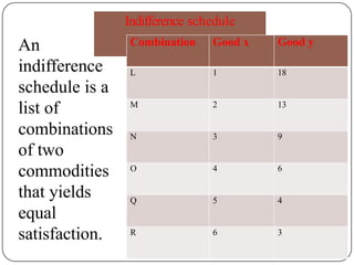
•An indifference Curve is drawn on the from the
indifferent schedule of the consumer.

3. Indifference schedule
An
indifference
schedule is a
list of
combinations
of two
commodities
that yields
equal
satisfaction.
Combination Good x Good y
L 1 18
M 2 13
N 3 9
O 4 6
Q 5 4
R 6 3

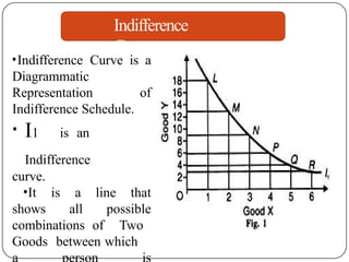
4. Indifference
Curve
•Indifference Curve is a
Diagrammatic
Representation of
Indifference Schedule.
• I1 is an
Indifference
curve.
•It is a line that
shows all possible
combinations of Two
Goods between which

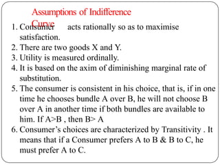
5. Assumptions of Indifference
Curve
1. Consumer acts rationally so as to maximise
satisfaction.
2. There are two goods X and Y.
3. Utility is measured ordinally.
4. It is based on the axim of diminishing marginal rate of
substitution.
5. The consumer is consistent in his choice, that is, if in one
time he chooses bundle A over B, he will not choose B
over A in another time if both bundles are available to
him. If A>B , then B> A
6. Consumer’s choices are characterized by Transitivity . It
means that if a Consumer prefers A to B & B to C, he
must prefer A to C.

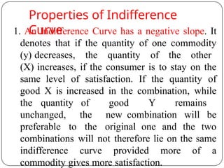
6. Properties of Indifference
Curve
1. An Indifference Curve has a negative slope. It
denotes that if the quantity of one commodity
(y) decreases, the quantity of the other
(X) increases, if the consumer is to stay on the
same level of satisfaction. If the quantity of
good X is increased in the combination, while
the quantity of good Y remains
unchanged, the new combination will be
preferable to the original one and the two
combinations will not therefore lie on the same
indifference curve provided more of a
commodity gives more satisfaction.

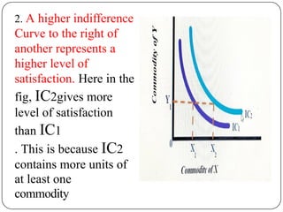
7. 2. A higher indifference
Curve to the right of
another represents a
higher level of
satisfaction. Here in the
fig, IC2gives more
level of satisfaction
than IC1
. This is because IC2
contains more units of
at least one
commodity

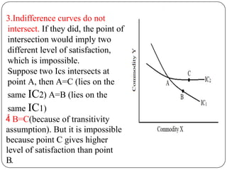
8. 3.Indifference curves do not
intersect. If they did, the point of
intersection would imply two
different level of satisfaction,
which is impossible.
Suppose two Ics intersects at
point A, then A=C (lies on the
same IC2) A=B (lies on the
same IC1)
 B=C(because of transitivity
assumption). But it is impossible
because point C gives higher
level of satisfaction than point
B.

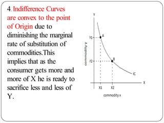
9. 4. Indifference Curves
are convex to the point
of Origin due to
diminishing the marginal
rate of substitution of
commodities.This
implies that as the
consumer gets more and
more of X he is ready to
sacrifice less and less of
Y.

10. 5.
Indifference
curves are not
necessarily
parallel to each
other. This is
because MRS may
differ for
different indifference
curves. If MRS differs
the slope of
indifference curves
also differs.