Improved techniques for grid mapping with rao blackwellized particle filters 번역
1.
Improved Techniques forGrid Mapping
With Rao-Blackwellized Particle Filters
도정찬
Girogio Grisestti, University of Freiburg, Dept of Computer Science
IEEE Transactions on Robotics, vol. 23, issue. 1, pp. 34-46, Feb. 2007
2.
요약
▪ Rao-blackwellized ParticleFilter(RBPF)기반의 SLAM 개발
▪ 아래 두가지 측면에서 장점을 가짐
- 정밀한 센서 측정 분포를 구하여 로봇 위치의 불확실성 줄임
- resampling 단계에서 파티클을 적절히 제거
▪ 실내외 환경에서 RBPF로 정밀한 grid map 작성
Abstraction
3.
Rao-Blackwellized Particle Filter이란?
▪Rao-Blackwellized Particle Filter(RBPF)
▪ A. Doucet이 2000년에 제안[1]
▪ SLAM를 위한 효율적인 방법
▪ Particle을 적절히 선별하여 SLAM 성능 향상
▪ 센서의 정밀도를 고려하여 자세 추정에 적합한 분포의 파티클 생성
▪ adaptive resampling을 통해 파티클을 잘못 제거하는 경우를 줄임
[1] A. Doucet, “Rao-Blackwellized particle filtering for dynamic Bayesian networks,” In proc. Of the Conf. on Uncertainty in Artificial Intelligencee (UAI), pp. 176-183,
Stanford, CA, USA, 2000.
Section 1. Introduction
4.
RBPF 방법
▪ pose에의존하는 파티클의 likelihood를 추정하여 생성
(이 때, pose는 odometry와 scan-matching procedure에서 구한다.)
▪ 현재 센서 측정으로 파티클 생성
(odometry에만 의존하는 경우보다 정밀)
▪ 이를 통해 두 장점이 있음
- 현재 관측에 대응하는 로봇의 위치를 구하여 정확한 지도를 작성하며 추정 오차를 줄임.
- adaptive resampling으로 필요한 파티클만 유지
▪ 본 논문은 이전[2]보다 개선된 RBPF 제안
▪ 실험 결과 큰 실내외 환경에서 정밀한 지도를 만들고, 계산할 파티클의 수를 줄임
[2] G. Grisetti, “Improving grid-based slam with Rao-Blackwellized particle filters by adaptive proposals and selective resampling,” In Proc. of the IEEE Int. Conf. on
Robotics & Automation(ICRA), pp 2443-2448, Barcelona, spain, 2005.
Section 1. Introduction
5.
논문 구조
▪ Section2. RBPF를 SLAM에 적용하는 방법
▪ Section 3. 본 논문에서 제안하는 방법
▪ Section 4. 구현 상세
▪ Section 6. 실험 내용
▪ Section 7. 결론
Section 1. Introduction
6.
Key idea ofslam using RBPF
▪ Murphy[3]에 따르면, RBPF를 SLAM에 적용시 key idea
=> 지도 m과 궤적 에 대한 결합확률 분포 를 추정
(이때, 관측 , 오도메트리 )
▪ RBPF는 아래와 같이 분해하여 사용함(로봇의 궤적을 추정 후, 이 궤적에 대한 지도 계산)
▪ 로봇의 궤적을 추정 후, 궤적에 대한 지도를 구함.
▪ 지도는 로봇의 위치에 의존하며 효율적으로 구하는 방법으로 Rao-Blackwellization(RB)이 사용됨
[3] k. Murphy. “Vayesian map learning in dynamic environments,” In Proc. Of the Conf. on Neural Information Processing Systems(NIPS), pp 1015-1021, Denvor, CO,
USA, 1999.
Section 2. Mapping with Rao-Blackwellized Particle Filters
7.
Mapping with RBPF
▪식 (1)의 map에 대한 사후확률 는 현재 자세에서 맵핑하여 구함
(이 때 , 를 알고 있어야 한다.)
▪ 잠재 궤적의 사후확률 을 구하기 위해 파티클 필터 사용
(파티클로 로봇의 궤적을 표현)
▪ 즉, 파티클로 로봇의 궤적 계산 -> 궤적에 대한 관측으로 지도 작성
Section 2. Mapping with Rao-Blackwellized Particle Filters
8.
Rao-Blackwellized Sampling ImportanceResampling Filter
▪ 대표적인 파티클 필터 알고리즘으로 Sampling Importance Resampling(SIR) filter
▪ Rao-Blackwellized SIR 필터는 아래의 4 단계로 처리 됨
1) Sampling : 분포 에 따라 파티클 를 샘플링하여 다음 파티클 을 구함
(이 때, 는 확률적 오도메트리 모션 모델의 분포를 사용함)
2) Importance Weighting : 각 파티클에는 importance sampling principle[아래의 식 (2)]에 따라 가중치 가 적용됨
(가중치의 합은 이 되지만 다음 상태의 목표 분포와 같지 않다.)
3) Resampling : 가중치에 따라 새 파티클들을 구함.(이 단계 후 모든 파티클의 가중치는 같게 됨)
4) Map estimation : 샘플로 구한 궤적 와 관측 로 추정 지도 를 계산
▪ 위를 구현하기 위해 새 관측 정보 얻을 때마다 처음부터 궤적의 가중치를 구해야 함.
즉, 주행 시간이 길어질수록 비효율적이게 됨.
SIR Filter의 initial sampling과 weight update
Section 2. Mapping with Rao-Blackwellized Particle Filters
9.
Compute the importanceweights
▪ Importance weights를 구하기 위해 아래의 식을 따르는 proposal 를 재귀 공식을 사용한다.(Doucet [7])
▪ 각 파티클들의 가중치는 식 (2)와 (3)을 이용하여 계산. (이때, 는 베이즈 룰을 따르는 정규화 factor)
▪ 대부분의 파티클 필터를 사용하는 어플리케이션은 식 (6)과 같이 재귀 구조를 사용함
▪ generic algorithm은 러닝 맵 사용, 파티클 필터는 리샘플링이 수행 될 때 proposal distribution이 어떻게 구하는가를 다룬다.
▪ 본 논문에서는 accurate proposal distribution과 adaptive resampling 방법에 대해 설명한다.
Section 2. Mapping with Rao-Blackwellized Particle Filters
10.
RBPF with ImprovedProposals and Adaptive Resampling
Section 3. RBPF with Improved Proposals and Adaptive Resampling
▪ 기존에 particle deptletion(low weighted particle)으로 인한 문제를 해결하고, improved proposal distribution을 구하는 다
양한 방법들이 제안됨[7,30,35]
▪ efficented particle filter implementation’s key idea
1) Computation of an improved proposal distribution 2) adaptive resampling technique
A. On the Improved Proposal Distribution
▪ Section 2의 prediction step에서 다음 파티클을 구하기 위해 proposal distribution π를 사용.
▪ proposal distribution이 target distribution을 잘 추정할수록 필터 성능도 좋아짐.
▪ 예시로 target distribution을 따르는 particle들을 만들 경우, 모든 particle의 importance weights가 똑같아짐.
-> resampling step이 필요 없음
11.
Proposal distribution usingodometry motion model
Section 3. RBPF with Improved Proposals and Adaptive Resampling
▪ 일반적인 PF 어플리케이션 [3,29]은 odometry motion model을 proposal distribution으로 사용.
-> 이 motion model은 대부분의 로봇에서 사용하기 쉬운 장점이 있음.
▪ importance weights는 observation model 을 사용하여 구할 수 있음
-> 식 (6)에서 motion model 로 π를 제거하면 아래의 식 (7), (8)처럼 정리되기 때문.
▪ 하지만 라이다처럼 odometry 보다 정밀한 센서를 사용하는 경우에는 odometry motion model 사용은 차선책이 된다.
(1) Computation of an imporved proposal distribution
12.
Meaningful area ofobservation/motion model likelihood
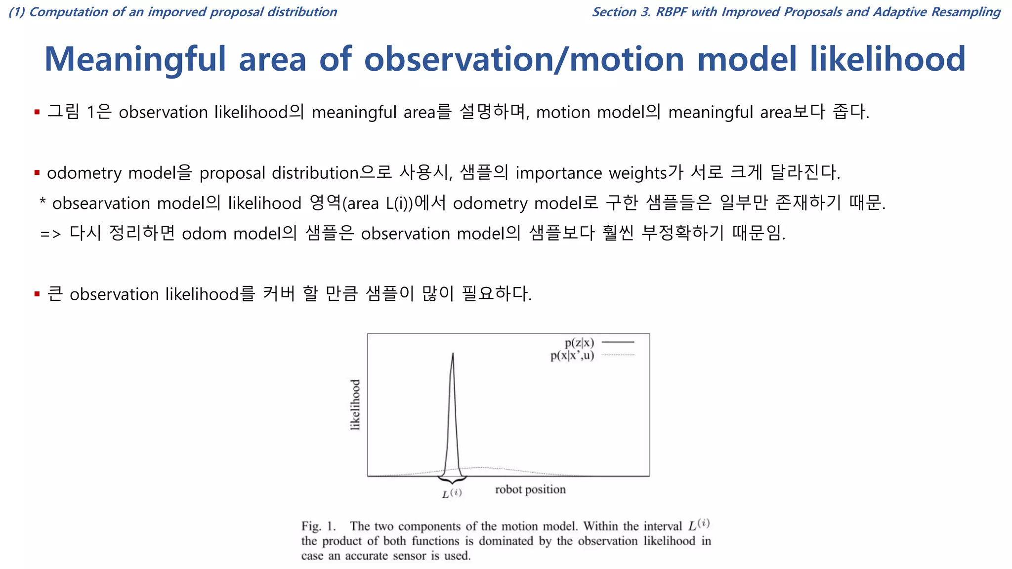
Section 3. RBPF with Improved Proposals and Adaptive Resampling
▪ 그림 1은 observation likelihood의 meaningful area를 설명하며, motion model의 meaningful area보다 좁다.
▪ odometry model을 proposal distribution으로 사용시, 샘플의 importance weights가 서로 크게 달라진다.
* obsearvation model의 likelihood 영역(area L(i))에서 odometry model로 구한 샘플들은 일부만 존재하기 때문.
=> 다시 정리하면 odom model의 샘플은 observation model의 샘플보다 훨씬 부정확하기 때문임.
▪ 큰 observation likelihood를 커버 할 만큼 샘플이 많이 필요하다.
(1) Computation of an imporved proposal distribution
13.
Smoothed likelihood function
Section3. RBPF with Improved Proposals and Adaptive Resampling
▪ 위치 추정에서 사용하는 일반적인 방법은 smoothed likelihood function이다.
▪ 이 방법은 meaningful area에 가까운 particle들이 너무 적은 low importance weight 값을 갖는 걸 방지한다.
* observation model의 likelihood가 smooth 해지면 관측 데이터로 위치를 잘 찾기 힘들어진다.
▪ 하지만 이 방법은 센서로 얻은 유용한 정보를 훼손시켜, 지도의 정확도를 떨어트린다.
▪ 개선 방법으로, 최근의 observation 를 proposal distribution과 통합하여 observation likelihood의 meaningful region에
서 sampling한다.
▪ 이 분포가 최적의 proposal distribution이 된다(by Doucet[5])
(1) Computation of an imporved proposal distribution
14.
Importance weights integratedwith recent observation
Section 3. RBPF with Improved Proposals and Adaptive Resampling
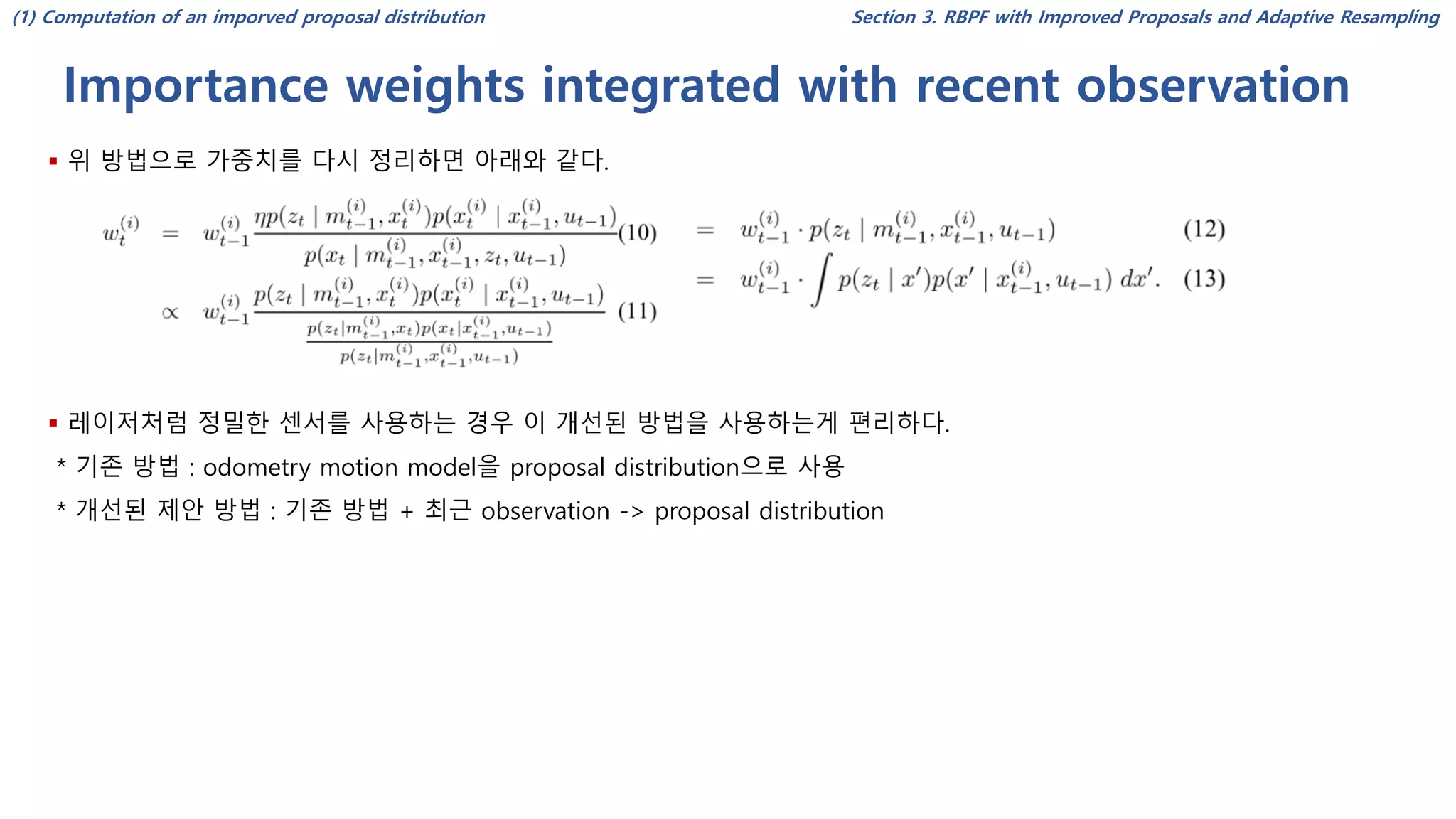
▪ 위 방법으로 가중치를 다시 정리하면 아래와 같다.
▪ 레이저처럼 정밀한 센서를 사용하는 경우 이 개선된 방법을 사용하는게 편리하다.
* 기존 방법 : odometry motion model을 proposal distribution으로 사용
* 개선된 제안 방법 : 기존 방법 + 최근 observation -> proposal distribution
(1) Computation of an imporved proposal distribution
15.
What is Rao-BlackwellizedParticle Filter?
Section 3. RBPF with Improved Proposals and Adaptive Resampling
▪ Landmark 기반 SLAM 문제에서 Montemerlo가 Rao-Blackwellized particle filter(RBPF)를 제안[26].
▪ RBPF는 가우시안 추정을 사용하여 개선된 분포를 만듬(improved proposal)
▪ 가우시안은 각 파티클들을 칼만 필터로 계산한다.
(이 방법은 지도를 특징으로 만들거나 특징 검출 에러가 가우시안의 형태가 따르는 경우 사용됨)
▪ 본 논문에서는 이 방법(RBPF)을 dense grid map에 사용한다. (landmark-based 대신)
(1) Computation of an imporved proposal distribution
16.
Efficient Computation ofthe Improved Proposal
Section 3. RBPF with Improved Proposals and Adaptive Resampling
▪ Grid Map 작성 시, observation likelihood function을 예측할 수 없기 때문에 추정 위치(informed proposal의 추정치)를 바
로 사용할 수 없다.
▪ 구한 분포의 추정형태(approximated form of the informed proposal)은 adaptive particle filter(APF)로 구할 수 있다 [35]
▪ 식 (9)를 따르는 샘플들의 추정치를 계산하여 APF가 적용된 proposal을 구한다.
* 이 때, 식 (9)는 motion model을 따르는 distribution보다 개선된 proposal distribution으로 recent sensor와 motion model
을 통합하여 구한다.
▪ APF를 SLAM에 적용하면, 우선 potential poses 의 집합을 샘플링해야한다.
(potential poses 는 i번째 particle의 motion model 로 구한다.
▪ 다음으로 optimal proposal의 approximation을 구하기 위해서는 observation likelihood로 샘플링된 potential poses에 가중
치를 주어야 한다.
(1) Computation of an imporved proposal distribution
17.
Adaptive Particle Filteras Approximation of the optimal proposal
Section 3. RBPF with Improved Proposals and Adaptive Resampling
▪ Observation likelihood가 pose samples 갯수 만큼 정점이 된다면, small area에서 high likelihood를 구하기 위해 많은 샘
플이 필요하다. (여기서 는 높은 motion model에서 샘플링 됨)
▪ 본 논문에서 target distribution의 주요한 특징은 최대치가 제한되고, 이 최대치는 하나만 존재한다.
- 이를 통해 초대치 안의 만 샘플링하며, 덜 중요한 meaningful region을 무시하여 계산량을 줄인다.
▪ 이전의 실험 [14]에서는 를 interval 과 constant k로 추정하였으며 아래의 식 (14)와 같다.
(2) Adaptive resampling technique
18.
Considering observation likelihoodand motion model
Section 3. RBPF with Improved Proposals and Adaptive Resampling
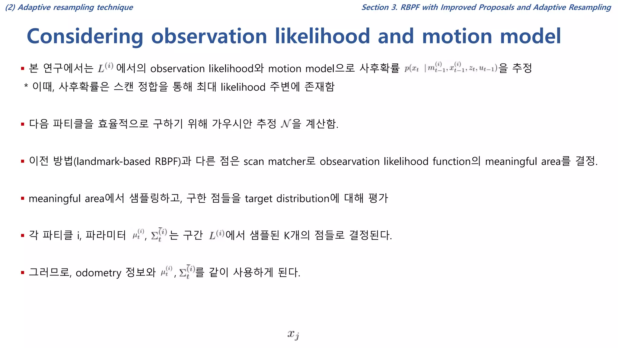
▪ 본 연구에서는 에서의 observation likelihood와 motion model으로 사후확률 을 추정
* 이때, 사후확률은 스캔 정합을 통해 최대 likelihood 주변에 존재함
▪ 다음 파티클을 효율적으로 구하기 위해 가우시안 추정 을 계산함.
▪ 이전 방법(landmark-based RBPF)과 다른 점은 scan matcher로 obsearvation likelihood function의 meaningful area를 결정.
▪ meaningful area에서 샘플링하고, 구한 점들을 target distribution에 대해 평가
▪ 각 파티클 i, 파라미터 , 는 구간 에서 샘플된 K개의 점들로 결정된다.
▪ 그러므로, odometry 정보와 , 를 같이 사용하게 된다.
(2) Adaptive resampling technique
19.
Gaussian parameters andweights
Section 3. RBPF with Improved Proposals and Adaptive Resampling
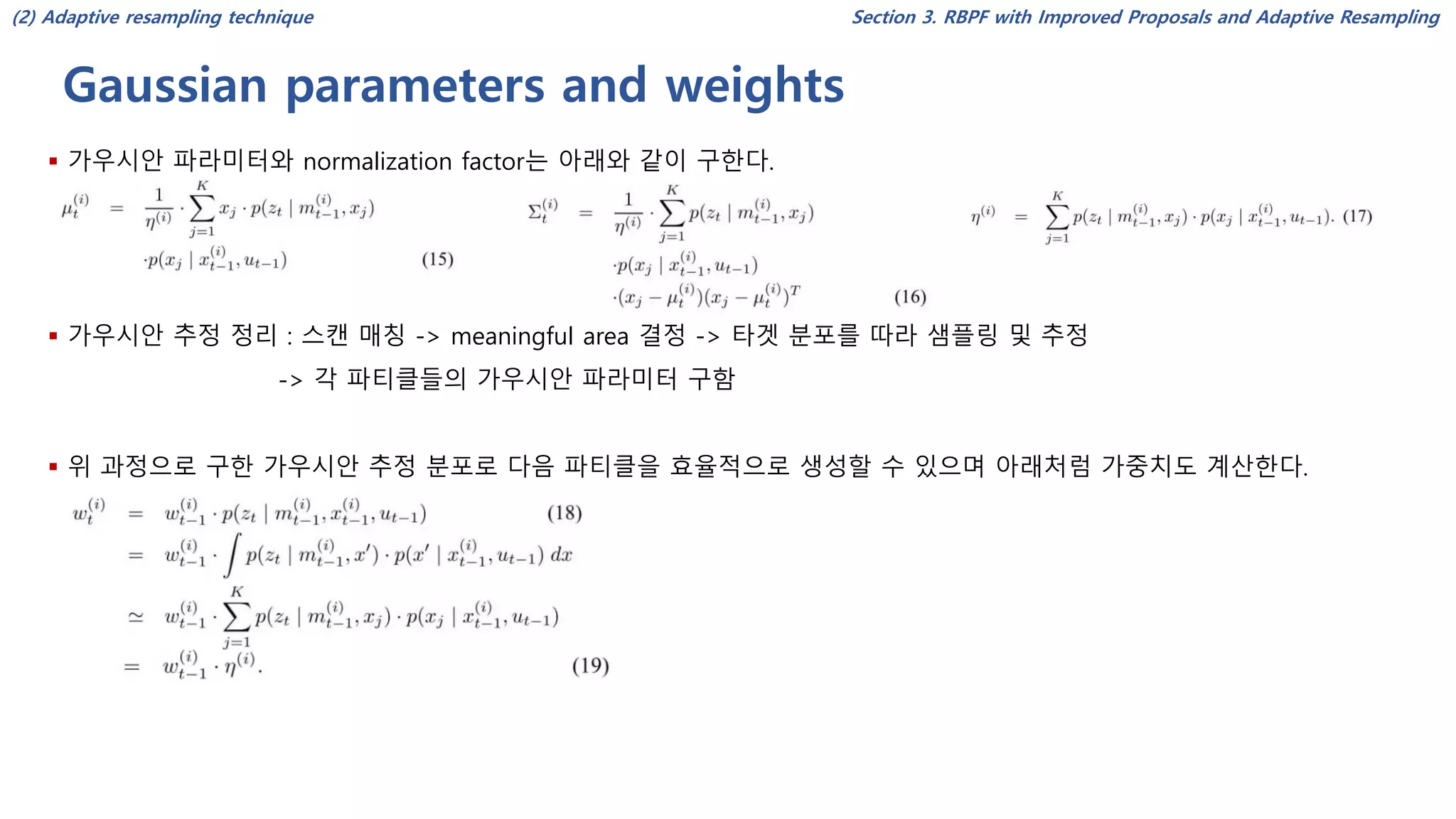
▪ 가우시안 파라미터와 normalization factor는 아래와 같이 구한다.
▪ 가우시안 추정 정리 : 스캔 매칭 -> meaningful area 결정 -> 타겟 분포를 따라 샘플링 및 추정
-> 각 파티클들의 가우시안 파라미터 구함
▪ 위 과정으로 구한 가우시안 추정 분포로 다음 파티클을 효율적으로 생성할 수 있으며 아래처럼 가중치도 계산한다.
(2) Adaptive resampling technique
20.
Discussion about theImproved Proposal
Section 3. RBPF with Improved Proposals and Adaptive Resampling
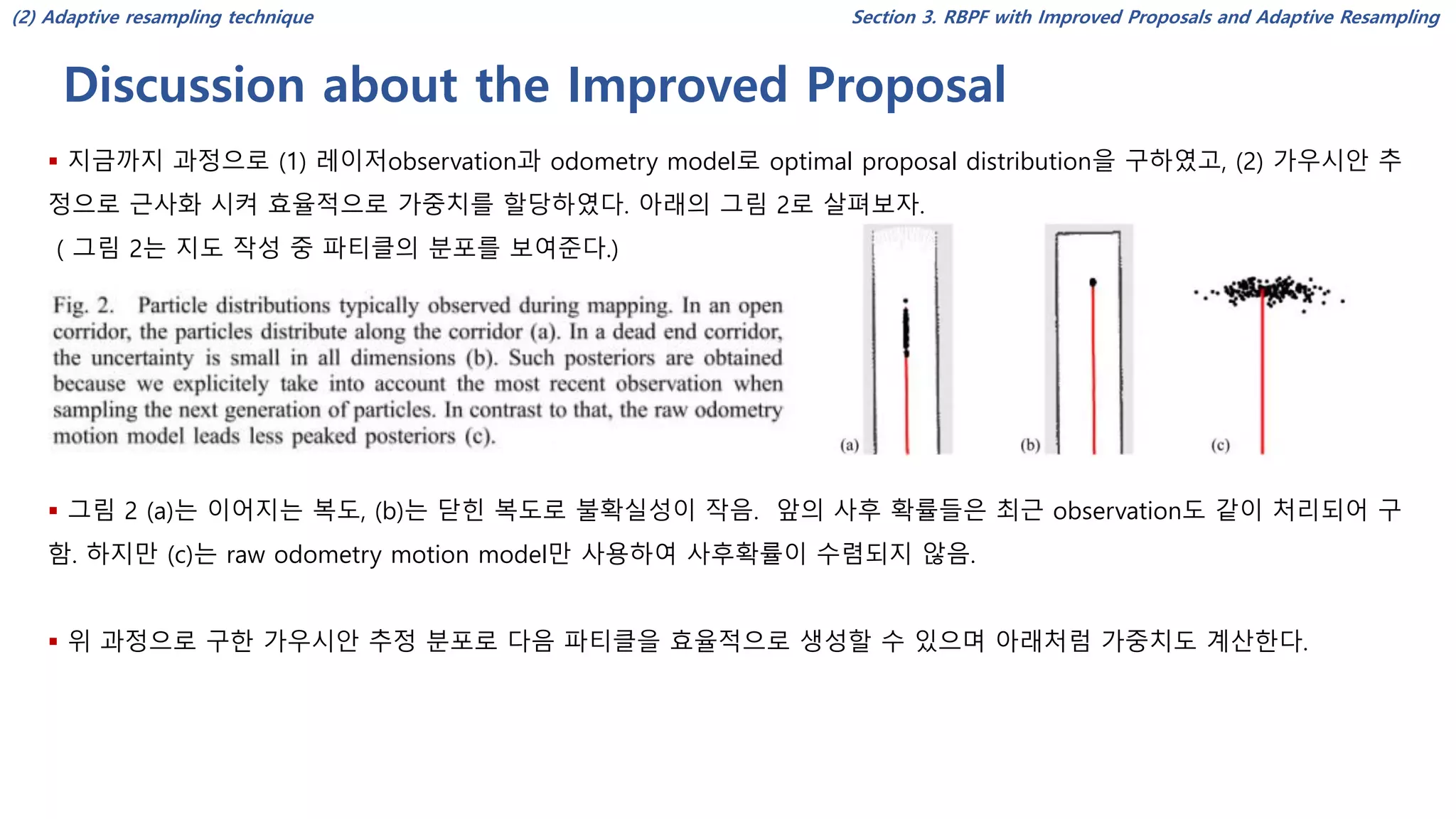
▪ 지금까지 과정으로 (1) 레이저observation과 odometry model로 optimal proposal distribution을 구하였고, (2) 가우시안 추
정으로 근사화 시켜 효율적으로 가중치를 할당하였다. 아래의 그림 2로 살펴보자.
( 그림 2는 지도 작성 중 파티클의 분포를 보여준다.)
▪ 그림 2 (a)는 이어지는 복도, (b)는 닫힌 복도로 불확실성이 작음. 앞의 사후 확률들은 최근 observation도 같이 처리되어 구
함. 하지만 (c)는 raw odometry motion model만 사용하여 사후확률이 수렴되지 않음.
▪ 위 과정으로 구한 가우시안 추정 분포로 다음 파티클을 효율적으로 생성할 수 있으며 아래처럼 가중치도 계산한다.
(2) Adaptive resampling technique
21.
Discussion about theImproved Proposal
Section 3. RBPF with Improved Proposals and Adaptive Resampling
▪ 위에서 설명하다 시피, scan-matcher를 observation likelihood의 meamingful area mode를 판단하는데 사용한다.
(여기서 말하는 mode란 single 혹은 multi-modal인지 말하는 것 같음)
▪ 이 방법에서는 important regions에서 샘플링 과정을 중심으로 본다.
▪ 대부분의 스캔 매칭 알고리즘은 map과 로봇 위치의 최초 추정(inital guess)가 주어질 때, observation likelihood가 최대가
된다.
▪ likelihood function이 multi-modal 이며 loop closing이 발생가능할때, scan macther는 파티클이 initial guess에 가까운 최대
치가 되도록 반환한다.
▪ 보통, single mode로 판단되면 likelihood function에서 additional maxima가 사라진다.
▪ 하지만 0.5m 씩 이동하거나 25도 씩 회전하도록 갱신하고 스캔 매처의 검색 범위를 제한하면, 이 분포는 가우시안 제안 분포
를 검출하기위해 data points를 샘플링할때 single mode만 존재한다.
(2) Adaptive resampling technique
22.
Discussion about theImproved Proposal
Section 3. RBPF with Improved Proposals and Adaptive Resampling
▪ 루프 폐쇄와 같은 상황에서, 스캔 매처의 시작점에 대한 initial guess는 loop에 다시 들어갈 때 각 파티클들이 다르므로
필터는 계속 다변으로 가정할수 있다.
▪ 그렇지만 역시 필터는 이론적으로 매우 과신할 수 있어, odometry가 노이즈에 크게 영향받으면 지도가 흩어질 수도 있다.
▪ 이 문제를 해결하기 위해 스캔 매처의 다변수 모드로 추적해야 하며 각 노드마다 샘플링 처리를 반복해야 한다.
▪ 그러나 본 실험에서 사용한 실제 로봇에서 이러한 문제는 발생하지 않았다.
▪ 필터링 동안 스캔 매칭 과정이 poosr observatio이나 이전과 현재 지도사이의 너무 작은 overlapping area로 실패 할 수 있
다. -> 이 때 그림 2 (c)에서 제안한 것과 같이 raw motion model을 사용한다.
(2) Adaptive resampling technique
23.
Adaptive Resampling
Section 3.RBPF with Improved Proposals and Adaptive Resampling
▪ resampling 단계는 파티클 필터 성능에 영향을 주며, 저 가중치 파티클들 대신 고 가중치 샘플로 대신한다.
▪ target distribution 추정에 몇개의 파티클로 리샘플링이 필요하며 줄여도 좋은 파티클들만 제거하도록 수행된다.
▪ 제거해야할 파티클을 찾기위한 기준으로 Liu[23]는 현재 파티클들이 목표 사후확률을 얼마나 잘 따르는지 추정하기 위해
effective sample size를 소개하였다.
▪ SLAM을 위해 Doucet[7]은 아래와 같이 공식화 하였으며, 파티클 i의 정규화 가중치를 의미한다.
▪ 를 살펴보면 만약 샘플이 target distribution을 이용해 만들어지면, importance weights가 서로 같아진다. 하지만 target
distribution을 잘못 추정할수록, importance weights의 분산은 커지게 된다.
▪ 는 importance weights의 분산치로 사용할수 있으며, 파티클들이 target posterior를 얼마나 잘 따르는지 평가하는데
좋다.
24.
Adaptive Resampling
Section 3.RBPF with Improved Proposals and Adaptive Resampling
▪ 본 연구의 알고리즘은 Doucet [7]의 제안한 방법으로 resampling step이 잘 수행되었는지 판단하게 된다.
▪ 매 시간 마다 가 임계치 N/2 보다 아래로 떨어지면 resampling을 수행하며, 이때 N는 전체 파티클의 갯수를 나타낸다.
▪ 실험에서 본 방법을 통해 좋은 파티클들이 사라지는 문제를 많이 줄이게 되었다.
(resampling을 필요할 때마다 수행되도록 하여 resampling 횟수가 줄었기 때문)
▪ 잘못된 target distribution으로 샘플을 생성하면, importance weights의 분산이 커지게 된다. 이 때 를 분산치로 사용
-> N_eff가 커지면 잘못된 target distribution, 줄어들면 좋은 target_distribution
▪ 로 resampling 수행 여부 판단. N_eff < N/2 => resampling(N is number of particle)
N_eff를 이용한 adaptive resampling 요약
25.
알고리즘 정리
Section 3.RBPF with Improved Proposals and Adaptive Resampling
- 전체적인 흐름은 알고리즘 1에 요약하였다. 새 측정 튜플 (u_t-1, z_t)가 매 시간마다 사용가능하고, 개별적인 파티클로 분포가 계산되어 파티
클 업데이트에 사용된다. 이 결과는 다음과 같다.
1) 파티클 i에 대한 로봇 위치 추정을 위해 최초의 추정 는 파티클에 대한 이전 자세 와 이전 필터 업데이트로 수집한 오도
메트리 측정 으로 구한다.(이 때, 연산자 는 표준 자세 연산 연산자가 된다 [24])
2) 최초의 추정 에서 시작한 지도 기반으로 스캔 매칭 알고리즘이 수행된다. 스캔 매처로 구한 결과는 의 주변에 있어야 한다. 만약 스
캔 매처가 실패시, 자세와 가중치가 모션 모델(3,4 단계가 무시되고)로 계산한다.
3) 샘플링 점들의 집합은 스캔 매처로 구한 자세 의 주위 구간 안에서 선별된다. 이 점들의 기반으로 제안된 분포의 평균과 공분산 행렬이
점들을 이용해서 샘플된 점 에서 타겟 분포 를 추정하여 구한다. 이 단계에서 가중치 요소 도 계산된다.
4)파티클 i의 새로운 자세 는 개선된 제안 분포의 가우시안 추정 으로 구한다.
5) 중요도 가중치를 갱신한다.
6) 파티클 i의 지도 이 그려진 자세 와 관측 에 따라 갱신된다.
- 다음 샘플들이 계산된 후 리샘플링 단계가 Neff의 값에 따라 수행된다.
![Rao-Blackwellized Particle Filter이란?
▪ Rao-Blackwellized Particle Filter(RBPF)
▪ A. Doucet이 2000년에 제안[1]
▪ SLAM를 위한 효율적인 방법
▪ Particle을 적절히 선별하여 SLAM 성능 향상
▪ 센서의 정밀도를 고려하여 자세 추정에 적합한 분포의 파티클 생성
▪ adaptive resampling을 통해 파티클을 잘못 제거하는 경우를 줄임
[1] A. Doucet, “Rao-Blackwellized particle filtering for dynamic Bayesian networks,” In proc. Of the Conf. on Uncertainty in Artificial Intelligencee (UAI), pp. 176-183,
Stanford, CA, USA, 2000.
Section 1. Introduction](https://image.slidesharecdn.com/improvedtechniquesforgridmappingwithrao-blackwellizedparticlefilters-190712003318/75/Improved-techniques-for-grid-mapping-with-rao-blackwellized-particle-filters-3-2048.jpg)
![RBPF 방법
▪ pose에 의존하는 파티클의 likelihood를 추정하여 생성
(이 때, pose는 odometry와 scan-matching procedure에서 구한다.)
▪ 현재 센서 측정으로 파티클 생성
(odometry에만 의존하는 경우보다 정밀)
▪ 이를 통해 두 장점이 있음
- 현재 관측에 대응하는 로봇의 위치를 구하여 정확한 지도를 작성하며 추정 오차를 줄임.
- adaptive resampling으로 필요한 파티클만 유지
▪ 본 논문은 이전[2]보다 개선된 RBPF 제안
▪ 실험 결과 큰 실내외 환경에서 정밀한 지도를 만들고, 계산할 파티클의 수를 줄임
[2] G. Grisetti, “Improving grid-based slam with Rao-Blackwellized particle filters by adaptive proposals and selective resampling,” In Proc. of the IEEE Int. Conf. on
Robotics & Automation(ICRA), pp 2443-2448, Barcelona, spain, 2005.
Section 1. Introduction](https://image.slidesharecdn.com/improvedtechniquesforgridmappingwithrao-blackwellizedparticlefilters-190712003318/75/Improved-techniques-for-grid-mapping-with-rao-blackwellized-particle-filters-4-2048.jpg)
![Key idea of slam using RBPF
▪ Murphy[3]에 따르면, RBPF를 SLAM에 적용시 key idea
=> 지도 m과 궤적 에 대한 결합확률 분포 를 추정
(이때, 관측 , 오도메트리 )
▪ RBPF는 아래와 같이 분해하여 사용함(로봇의 궤적을 추정 후, 이 궤적에 대한 지도 계산)
▪ 로봇의 궤적을 추정 후, 궤적에 대한 지도를 구함.
▪ 지도는 로봇의 위치에 의존하며 효율적으로 구하는 방법으로 Rao-Blackwellization(RB)이 사용됨
[3] k. Murphy. “Vayesian map learning in dynamic environments,” In Proc. Of the Conf. on Neural Information Processing Systems(NIPS), pp 1015-1021, Denvor, CO,
USA, 1999.
Section 2. Mapping with Rao-Blackwellized Particle Filters](https://image.slidesharecdn.com/improvedtechniquesforgridmappingwithrao-blackwellizedparticlefilters-190712003318/75/Improved-techniques-for-grid-mapping-with-rao-blackwellized-particle-filters-6-2048.jpg)
![Rao-Blackwellized Sampling Importance Resampling Filter
▪ 대표적인 파티클 필터 알고리즘으로 Sampling Importance Resampling(SIR) filter
▪ Rao-Blackwellized SIR 필터는 아래의 4 단계로 처리 됨
1) Sampling : 분포 에 따라 파티클 를 샘플링하여 다음 파티클 을 구함
(이 때, 는 확률적 오도메트리 모션 모델의 분포를 사용함)
2) Importance Weighting : 각 파티클에는 importance sampling principle[아래의 식 (2)]에 따라 가중치 가 적용됨
(가중치의 합은 이 되지만 다음 상태의 목표 분포와 같지 않다.)
3) Resampling : 가중치에 따라 새 파티클들을 구함.(이 단계 후 모든 파티클의 가중치는 같게 됨)
4) Map estimation : 샘플로 구한 궤적 와 관측 로 추정 지도 를 계산
▪ 위를 구현하기 위해 새 관측 정보 얻을 때마다 처음부터 궤적의 가중치를 구해야 함.
즉, 주행 시간이 길어질수록 비효율적이게 됨.
SIR Filter의 initial sampling과 weight update
Section 2. Mapping with Rao-Blackwellized Particle Filters](https://image.slidesharecdn.com/improvedtechniquesforgridmappingwithrao-blackwellizedparticlefilters-190712003318/75/Improved-techniques-for-grid-mapping-with-rao-blackwellized-particle-filters-8-2048.jpg)
![Compute the importance weights
▪ Importance weights를 구하기 위해 아래의 식을 따르는 proposal 를 재귀 공식을 사용한다.(Doucet [7])
▪ 각 파티클들의 가중치는 식 (2)와 (3)을 이용하여 계산. (이때, 는 베이즈 룰을 따르는 정규화 factor)
▪ 대부분의 파티클 필터를 사용하는 어플리케이션은 식 (6)과 같이 재귀 구조를 사용함
▪ generic algorithm은 러닝 맵 사용, 파티클 필터는 리샘플링이 수행 될 때 proposal distribution이 어떻게 구하는가를 다룬다.
▪ 본 논문에서는 accurate proposal distribution과 adaptive resampling 방법에 대해 설명한다.
Section 2. Mapping with Rao-Blackwellized Particle Filters](https://image.slidesharecdn.com/improvedtechniquesforgridmappingwithrao-blackwellizedparticlefilters-190712003318/75/Improved-techniques-for-grid-mapping-with-rao-blackwellized-particle-filters-9-2048.jpg)
![RBPF with Improved Proposals and Adaptive Resampling
Section 3. RBPF with Improved Proposals and Adaptive Resampling
▪ 기존에 particle deptletion(low weighted particle)으로 인한 문제를 해결하고, improved proposal distribution을 구하는 다
양한 방법들이 제안됨[7,30,35]
▪ efficented particle filter implementation’s key idea
1) Computation of an improved proposal distribution 2) adaptive resampling technique
A. On the Improved Proposal Distribution
▪ Section 2의 prediction step에서 다음 파티클을 구하기 위해 proposal distribution π를 사용.
▪ proposal distribution이 target distribution을 잘 추정할수록 필터 성능도 좋아짐.
▪ 예시로 target distribution을 따르는 particle들을 만들 경우, 모든 particle의 importance weights가 똑같아짐.
-> resampling step이 필요 없음](https://image.slidesharecdn.com/improvedtechniquesforgridmappingwithrao-blackwellizedparticlefilters-190712003318/75/Improved-techniques-for-grid-mapping-with-rao-blackwellized-particle-filters-10-2048.jpg)
![Proposal distribution using odometry motion model
Section 3. RBPF with Improved Proposals and Adaptive Resampling
▪ 일반적인 PF 어플리케이션 [3,29]은 odometry motion model을 proposal distribution으로 사용.
-> 이 motion model은 대부분의 로봇에서 사용하기 쉬운 장점이 있음.
▪ importance weights는 observation model 을 사용하여 구할 수 있음
-> 식 (6)에서 motion model 로 π를 제거하면 아래의 식 (7), (8)처럼 정리되기 때문.
▪ 하지만 라이다처럼 odometry 보다 정밀한 센서를 사용하는 경우에는 odometry motion model 사용은 차선책이 된다.
(1) Computation of an imporved proposal distribution](https://image.slidesharecdn.com/improvedtechniquesforgridmappingwithrao-blackwellizedparticlefilters-190712003318/75/Improved-techniques-for-grid-mapping-with-rao-blackwellized-particle-filters-11-2048.jpg)
![Smoothed likelihood function
Section 3. RBPF with Improved Proposals and Adaptive Resampling
▪ 위치 추정에서 사용하는 일반적인 방법은 smoothed likelihood function이다.
▪ 이 방법은 meaningful area에 가까운 particle들이 너무 적은 low importance weight 값을 갖는 걸 방지한다.
* observation model의 likelihood가 smooth 해지면 관측 데이터로 위치를 잘 찾기 힘들어진다.
▪ 하지만 이 방법은 센서로 얻은 유용한 정보를 훼손시켜, 지도의 정확도를 떨어트린다.
▪ 개선 방법으로, 최근의 observation 를 proposal distribution과 통합하여 observation likelihood의 meaningful region에
서 sampling한다.
▪ 이 분포가 최적의 proposal distribution이 된다(by Doucet[5])
(1) Computation of an imporved proposal distribution](https://image.slidesharecdn.com/improvedtechniquesforgridmappingwithrao-blackwellizedparticlefilters-190712003318/75/Improved-techniques-for-grid-mapping-with-rao-blackwellized-particle-filters-13-2048.jpg)
![What is Rao-Blackwellized Particle Filter?
Section 3. RBPF with Improved Proposals and Adaptive Resampling
▪ Landmark 기반 SLAM 문제에서 Montemerlo가 Rao-Blackwellized particle filter(RBPF)를 제안[26].
▪ RBPF는 가우시안 추정을 사용하여 개선된 분포를 만듬(improved proposal)
▪ 가우시안은 각 파티클들을 칼만 필터로 계산한다.
(이 방법은 지도를 특징으로 만들거나 특징 검출 에러가 가우시안의 형태가 따르는 경우 사용됨)
▪ 본 논문에서는 이 방법(RBPF)을 dense grid map에 사용한다. (landmark-based 대신)
(1) Computation of an imporved proposal distribution](https://image.slidesharecdn.com/improvedtechniquesforgridmappingwithrao-blackwellizedparticlefilters-190712003318/75/Improved-techniques-for-grid-mapping-with-rao-blackwellized-particle-filters-15-2048.jpg)
![Efficient Computation of the Improved Proposal
Section 3. RBPF with Improved Proposals and Adaptive Resampling
▪ Grid Map 작성 시, observation likelihood function을 예측할 수 없기 때문에 추정 위치(informed proposal의 추정치)를 바
로 사용할 수 없다.
▪ 구한 분포의 추정형태(approximated form of the informed proposal)은 adaptive particle filter(APF)로 구할 수 있다 [35]
▪ 식 (9)를 따르는 샘플들의 추정치를 계산하여 APF가 적용된 proposal을 구한다.
* 이 때, 식 (9)는 motion model을 따르는 distribution보다 개선된 proposal distribution으로 recent sensor와 motion model
을 통합하여 구한다.
▪ APF를 SLAM에 적용하면, 우선 potential poses 의 집합을 샘플링해야한다.
(potential poses 는 i번째 particle의 motion model 로 구한다.
▪ 다음으로 optimal proposal의 approximation을 구하기 위해서는 observation likelihood로 샘플링된 potential poses에 가중
치를 주어야 한다.
(1) Computation of an imporved proposal distribution](https://image.slidesharecdn.com/improvedtechniquesforgridmappingwithrao-blackwellizedparticlefilters-190712003318/75/Improved-techniques-for-grid-mapping-with-rao-blackwellized-particle-filters-16-2048.jpg)
![Adaptive Particle Filter as Approximation of the optimal proposal
Section 3. RBPF with Improved Proposals and Adaptive Resampling
▪ Observation likelihood가 pose samples 갯수 만큼 정점이 된다면, small area에서 high likelihood를 구하기 위해 많은 샘
플이 필요하다. (여기서 는 높은 motion model에서 샘플링 됨)
▪ 본 논문에서 target distribution의 주요한 특징은 최대치가 제한되고, 이 최대치는 하나만 존재한다.
- 이를 통해 초대치 안의 만 샘플링하며, 덜 중요한 meaningful region을 무시하여 계산량을 줄인다.
▪ 이전의 실험 [14]에서는 를 interval 과 constant k로 추정하였으며 아래의 식 (14)와 같다.
(2) Adaptive resampling technique](https://image.slidesharecdn.com/improvedtechniquesforgridmappingwithrao-blackwellizedparticlefilters-190712003318/75/Improved-techniques-for-grid-mapping-with-rao-blackwellized-particle-filters-17-2048.jpg)
![Adaptive Resampling
Section 3. RBPF with Improved Proposals and Adaptive Resampling
▪ resampling 단계는 파티클 필터 성능에 영향을 주며, 저 가중치 파티클들 대신 고 가중치 샘플로 대신한다.
▪ target distribution 추정에 몇개의 파티클로 리샘플링이 필요하며 줄여도 좋은 파티클들만 제거하도록 수행된다.
▪ 제거해야할 파티클을 찾기위한 기준으로 Liu[23]는 현재 파티클들이 목표 사후확률을 얼마나 잘 따르는지 추정하기 위해
effective sample size를 소개하였다.
▪ SLAM을 위해 Doucet[7]은 아래와 같이 공식화 하였으며, 파티클 i의 정규화 가중치를 의미한다.
▪ 를 살펴보면 만약 샘플이 target distribution을 이용해 만들어지면, importance weights가 서로 같아진다. 하지만 target
distribution을 잘못 추정할수록, importance weights의 분산은 커지게 된다.
▪ 는 importance weights의 분산치로 사용할수 있으며, 파티클들이 target posterior를 얼마나 잘 따르는지 평가하는데
좋다.](https://image.slidesharecdn.com/improvedtechniquesforgridmappingwithrao-blackwellizedparticlefilters-190712003318/75/Improved-techniques-for-grid-mapping-with-rao-blackwellized-particle-filters-23-2048.jpg)
![Adaptive Resampling
Section 3. RBPF with Improved Proposals and Adaptive Resampling
▪ 본 연구의 알고리즘은 Doucet [7]의 제안한 방법으로 resampling step이 잘 수행되었는지 판단하게 된다.
▪ 매 시간 마다 가 임계치 N/2 보다 아래로 떨어지면 resampling을 수행하며, 이때 N는 전체 파티클의 갯수를 나타낸다.
▪ 실험에서 본 방법을 통해 좋은 파티클들이 사라지는 문제를 많이 줄이게 되었다.
(resampling을 필요할 때마다 수행되도록 하여 resampling 횟수가 줄었기 때문)
▪ 잘못된 target distribution으로 샘플을 생성하면, importance weights의 분산이 커지게 된다. 이 때 를 분산치로 사용
-> N_eff가 커지면 잘못된 target distribution, 줄어들면 좋은 target_distribution
▪ 로 resampling 수행 여부 판단. N_eff < N/2 => resampling(N is number of particle)
N_eff를 이용한 adaptive resampling 요약](https://image.slidesharecdn.com/improvedtechniquesforgridmappingwithrao-blackwellizedparticlefilters-190712003318/75/Improved-techniques-for-grid-mapping-with-rao-blackwellized-particle-filters-24-2048.jpg)
![알고리즘 정리
Section 3. RBPF with Improved Proposals and Adaptive Resampling
- 전체적인 흐름은 알고리즘 1에 요약하였다. 새 측정 튜플 (u_t-1, z_t)가 매 시간마다 사용가능하고, 개별적인 파티클로 분포가 계산되어 파티
클 업데이트에 사용된다. 이 결과는 다음과 같다.
1) 파티클 i에 대한 로봇 위치 추정을 위해 최초의 추정 는 파티클에 대한 이전 자세 와 이전 필터 업데이트로 수집한 오도
메트리 측정 으로 구한다.(이 때, 연산자 는 표준 자세 연산 연산자가 된다 [24])
2) 최초의 추정 에서 시작한 지도 기반으로 스캔 매칭 알고리즘이 수행된다. 스캔 매처로 구한 결과는 의 주변에 있어야 한다. 만약 스
캔 매처가 실패시, 자세와 가중치가 모션 모델(3,4 단계가 무시되고)로 계산한다.
3) 샘플링 점들의 집합은 스캔 매처로 구한 자세 의 주위 구간 안에서 선별된다. 이 점들의 기반으로 제안된 분포의 평균과 공분산 행렬이
점들을 이용해서 샘플된 점 에서 타겟 분포 를 추정하여 구한다. 이 단계에서 가중치 요소 도 계산된다.
4)파티클 i의 새로운 자세 는 개선된 제안 분포의 가우시안 추정 으로 구한다.
5) 중요도 가중치를 갱신한다.
6) 파티클 i의 지도 이 그려진 자세 와 관측 에 따라 갱신된다.
- 다음 샘플들이 계산된 후 리샘플링 단계가 Neff의 값에 따라 수행된다.](https://image.slidesharecdn.com/improvedtechniquesforgridmappingwithrao-blackwellizedparticlefilters-190712003318/75/Improved-techniques-for-grid-mapping-with-rao-blackwellized-particle-filters-25-2048.jpg)


![[0806 박민근] 림 라이팅(rim lighting)](https://cdn.slidesharecdn.com/ss_thumbnails/0806rimlighting-110808045739-phpapp01-thumbnail.jpg?width=640&height=640&fit=bounds)


![[1023 박민수] 깊이_버퍼_그림자](https://cdn.slidesharecdn.com/ss_thumbnails/1023-101109093507-phpapp01-thumbnail.jpg?width=640&height=640&fit=bounds)


![[IGC 2016] 넷게임즈 김영희 - Unreal4를 사용해 모바일 프로젝트 제작하기](https://cdn.slidesharecdn.com/ss_thumbnails/igcppt-161008143730-thumbnail.jpg?width=640&height=640&fit=bounds)


![2017 12 09_데브루키_리얼타임 렌더링_입문편(3차원 그래픽스[저자 : 한정현] 참조)](https://cdn.slidesharecdn.com/ss_thumbnails/20171209-171227014347-thumbnail.jpg?width=640&height=640&fit=bounds)


![[밑러닝] Chap06 학습관련기술들](https://cdn.slidesharecdn.com/ss_thumbnails/chap06-171119110341-thumbnail.jpg?width=640&height=640&fit=bounds)


![[KCC 2019] CNN 기반 물체 파지를 위한 위치 탐색 (CNN-based Grasping Box Detection)](https://cdn.slidesharecdn.com/ss_thumbnails/kcc2019-190701011353-thumbnail.jpg?width=640&height=640&fit=bounds)
![[컴퓨터비전과 인공지능] 10. 신경망 학습하기 파트 1 - 2. 데이터 전처리](https://cdn.slidesharecdn.com/ss_thumbnails/lec10trainingneuralnetworkspart12datapreprocessing-210223065837-thumbnail.jpg?width=640&height=640&fit=bounds)
![[컴퓨터비전과 인공지능] 10. 신경망 학습하기 파트 1 - 1. 활성화 함수](https://cdn.slidesharecdn.com/ss_thumbnails/lec10trainingneuralnetworks1activationfunction-210221112518-thumbnail.jpg?width=640&height=640&fit=bounds)
![[컴퓨터비전과 인공지능] 8. 합성곱 신경망 아키텍처 5 - Others](https://cdn.slidesharecdn.com/ss_thumbnails/lec8convolutionnetworksarcitecture5others-210215060452-thumbnail.jpg?width=640&height=640&fit=bounds)
![[컴퓨터비전과 인공지능] 8. 합성곱 신경망 아키텍처 4 - ResNet](https://cdn.slidesharecdn.com/ss_thumbnails/lec8convolutionnetworksarcitecture4resnet-210214112234-thumbnail.jpg?width=640&height=640&fit=bounds)
![[컴퓨터비전과 인공지능] 8. 합성곱 신경망 아키텍처 3 - GoogLeNet](https://cdn.slidesharecdn.com/ss_thumbnails/lec8convolutionnetworksarcitecture3googlenet-210214112100-thumbnail.jpg?width=640&height=640&fit=bounds)
![[컴퓨터비전과 인공지능] 8. 합성곱 신경망 아키텍처 2 - ZFNet, VGG-16](https://cdn.slidesharecdn.com/ss_thumbnails/lec8convolutionnetworksarcitecture2zfnetvgg16-210213163140-thumbnail.jpg?width=640&height=640&fit=bounds)
![[컴퓨터비전과 인공지능] 8. 합성곱 신경망 아키텍처 1 - 알렉스넷](https://cdn.slidesharecdn.com/ss_thumbnails/lec8convolutionnetworksarcitecture1alexnet-210213163008-thumbnail.jpg?width=640&height=640&fit=bounds)
![[컴퓨터비전과 인공지능] 7. 합성곱 신경망 2](https://cdn.slidesharecdn.com/ss_thumbnails/lec7convolutionnetworks2-210213150820-thumbnail.jpg?width=640&height=640&fit=bounds)
![[컴퓨터비전과 인공지능] 7. 합성곱 신경망 1](https://cdn.slidesharecdn.com/ss_thumbnails/lec7convolutionnetwork-210207104334-thumbnail.jpg?width=640&height=640&fit=bounds)
![[컴퓨터비전과 인공지능] 6. 역전파 2](https://cdn.slidesharecdn.com/ss_thumbnails/lec6backpropagation2-210203225156-thumbnail.jpg?width=640&height=640&fit=bounds)
![[컴퓨터비전과 인공지능] 6. 역전파 1](https://cdn.slidesharecdn.com/ss_thumbnails/lec6backpropagation-210201173541-thumbnail.jpg?width=640&height=640&fit=bounds)
![[컴퓨터비전과 인공지능] 5. 신경망 2 - 신경망 근사화와 컨벡스 함수](https://cdn.slidesharecdn.com/ss_thumbnails/neuralnetwork2-210128174417-thumbnail.jpg?width=640&height=640&fit=bounds)
![[리트코드 문제 풀기] 연결 리스트](https://cdn.slidesharecdn.com/ss_thumbnails/127coma-210127082946-thumbnail.jpg?width=640&height=640&fit=bounds)
![[컴퓨터비전과 인공지능] 5. 신경망](https://cdn.slidesharecdn.com/ss_thumbnails/lec5neuralnetwork-210125014802-thumbnail.jpg?width=640&height=640&fit=bounds)
![[리트코드 문제 풀기] 배열](https://cdn.slidesharecdn.com/ss_thumbnails/leetcode-210119155410-thumbnail.jpg?width=640&height=640&fit=bounds)
![[컴퓨터비전과 인공지능] 4. 최적화](https://cdn.slidesharecdn.com/ss_thumbnails/lec4202101181335optimization-210119155221-thumbnail.jpg?width=640&height=640&fit=bounds)
![[컴퓨터비전과 인공지능] 3. 선형 분류기 : 손실 함수와 규제](https://cdn.slidesharecdn.com/ss_thumbnails/202101112200linearclassifier2-210111130805-thumbnail.jpg?width=640&height=640&fit=bounds)
![[컴퓨터비전과 인공지능] 3. 선형 분류 : 선형 분류기 일부](https://cdn.slidesharecdn.com/ss_thumbnails/202101111400linearclassifier-210111060058-thumbnail.jpg?width=640&height=640&fit=bounds)

