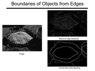
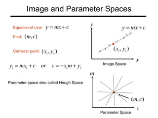
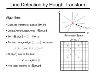
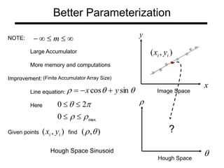
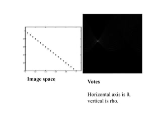
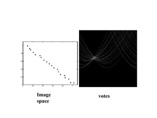
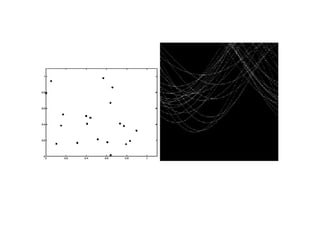
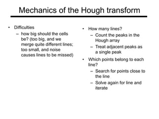
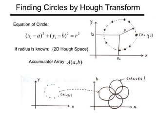
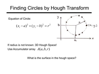
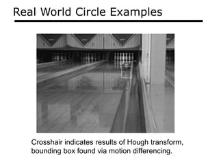
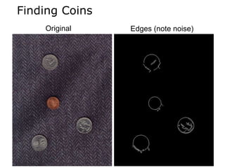
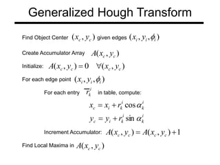
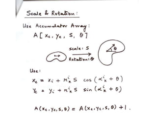
The document discusses boundary detection and the Hough transform. It covers topics like edge tracking methods, fitting lines and curves to edges, and the mechanics of the Hough transform. The Hough transform is an algorithm that can be used to detect simple shapes like lines and circles. It works by having each edge point in an image "vote" for possible shape parameters, and finding peaks in a parameter space accumulator to detect shapes. The document provides examples of using the Hough transform to detect lines and circles in images.

1. Boundary Detection:
Hough Transform

2. Boundaries of Objects
Marked by many users
http://www.eecs.berkeley.edu/Research/Projects/CS/vision/grouping/segbench/bench/html/images.html

3. Boundaries of Objects from Edges
Brightness Gradient (Edge detection)
• Missing edge continuity, many edges

4. Boundaries of Objects from Edges
Multi-scale Brightness Gradient
• But, low strength edges may be very important

5. Boundaries of Objects from Edges
Image
Machine Edge Detection
Human Boundary Marking

6. Boundaries in Medical Imaging
Detection of cancerous regions.

7. Boundaries in Ultrasound Images
Hard to detect in the presence of large amount of speckle noise

8. Boundaries of Objects
Sometimes hard even for humans!

9. Topics
• Preprocessing Edge Images
• Edge Tracking Methods
• Fitting Lines and Curves to Edges
• The Hough Transform

10. Preprocessing Edge Images
Image
Edge detection
and Thresholding
Noisy edge image
Incomplete boundaries
Shrink and Expand
Thinning

11. Edge Tracking Methods
Adjusting a priori Boundaries:
Given: Approximate Location of Boundary
Task: Find Accurate Location of Boundary
• Search for STRONG EDGES along normals to approximate boundary.
• Fit curve (eg., polynomials) to strong edges.

12. Edge Tracking Methods
Divide and Conquer:
Given: Boundary lies between points A and B
Task: Find Boundary
• Connect A and B with Line
• Find strongest edge along line bisector
• Use edge point as break point
• Repeat

13. Fitting Lines to Edges (Least Squares)
c
mx
y 

)
,
( i
i y
x
y
x
Given: Many pairs
Find: Parameters
Minimize: Average square distance:
Using:
)
,
( i
i y
x
)
,
( c
m




i
i
i
N
c
mx
y
E
2
)
(
N
y
y i
i


N
x
x i
i



14. Problem with Parameterization
y
x
Line that minimizes E!!
Solution: Use a different parameterization
(same as the one we used in computing Minimum Moment of Inertia)
Note: Error E must be formulated carefully!
 


i
i
i y
x
N
E 2
)
sin
cos
(
1




15. Line fitting can be max.
likelihood - but choice of
model is important

16. Curve Fitting
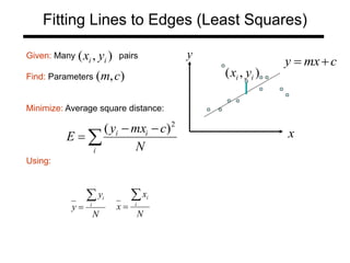
y
x
Find Polynomial:
that best fits the given points
Minimize:
Using:
Note: is LINEAR in the parameters (a, b, c, d)
)
,
( i
i y
x
d
cx
bx
ax
x
f
y 



 2
3
)
(
 



i
i
i
i
i d
cx
bx
ax
y
N
2
2
3
)]
(
[
1
0
,
0
,
0
,
0 











d
E
c
E
b
E
a
E
)
(x
f

17. Line Grouping Problem
Slide credit: David Jacobs

18. This is difficult because of:
• Extraneous data: clutter or multiple models
– We do not know what is part of the model?
– Can we pull out models with a few parts from much
larger amounts of background clutter?
• Missing data: only some parts of model are present
• Noise
• Cost:
– It is not feasible to check all combinations of features
by fitting a model to each possible subset

19. Hough Transform
• Elegant method for direct object recognition
• Edges need not be connected
• Complete object need not be visible
• Key Idea: Edges VOTE for the possible model

20. Image and Parameter Spaces
c
mx
y 

)
,
( i
i y
x
y
x
Equation of Line:
Find:
Consider point:
c
mx
y 

)
,
( c
m
)
,
( i
i y
x
i
i
i
i y
m
x
c
or
c
mx
y 




m
c
)
,
( c
m
Image Space
Parameter Space
Parameter space also called Hough Space

21. Line Detection by Hough Transform
y
x
)
,
( c
m
Parameter Space
1 1
1 1
1 1
2
1 1
1 1
1 1
)
,
( c
m
A
Algorithm:
• Quantize Parameter Space
• Create Accumulator Array
• Set
• For each image edge increment:
• If lies on the line:
• Find local maxima in
)
,
( c
m
)
,
( c
m
A
c
m
c
m
A ,
0
)
,
( 

)
,
( i
i y
x
1
)
,
(
)
,
( 
 c
m
A
c
m
A
)
,
( c
m
)
,
( c
m
A
i
i y
m
x
c 



22. Better Parameterization
NOTE:
Large Accumulator
More memory and computations
Improvement:
Line equation:
Here
Given points find




 m


 sin
cos y
x 


max
0
2
0








(Finite Accumulator Array Size)
)
,
( i
i y
x )
,
( 

)
,
( i
i y
x
y
x
Image Space


Hough Space
?
Hough Space Sinusoid

23. Image space
Votes
Horizontal axis is θ,
vertical is rho.

24. Image
space
votes

26. Mechanics of the Hough transform
• Difficulties
– how big should the cells
be? (too big, and we
merge quite different lines;
too small, and noise
causes lines to be missed)
• How many lines?
– Count the peaks in the
Hough array
– Treat adjacent peaks as
a single peak
• Which points belong to each
line?
– Search for points close to
the line
– Solve again for line and
iterate

27. Fewer votes land in a single bin when noise increases.

28. Adding more clutter increases number of bins with false peaks.

29. Real World Example
Original Edge
Detection
Found Lines
Parameter Space

30. Finding Circles by Hough Transform
Equation of Circle:
2
2
2
)
(
)
( r
b
y
a
x i
i 



If radius is known:
)
,
( b
a
A
Accumulator Array
(2D Hough Space)

31. Finding Circles by Hough Transform
Equation of Circle:
2
2
2
)
(
)
( r
b
y
a
x i
i 



If radius is not known: 3D Hough Space!
Use Accumulator array )
,
,
( r
b
a
A
What is the surface in the hough space?

32. Using Gradient Information
• Gradient information can save lot of computation:
Edge Location
Edge Direction
Need to increment only one point in Accumulator!!
i

)
,
( i
i y
x
Assume radius is known:


sin
cos
r
y
b
r
x
a





33. Real World Circle Examples
Crosshair indicates results of Hough transform,
bounding box found via motion differencing.

34. Finding Coins
Original Edges (note noise)

35. Finding Coins (Continued)
Penn
y
Quarters

36. Finding Coins (Continued)
Coin finding sample images
Note that because
the quarters and
penny are different
sizes, a different
Hough transform
(with separate
accumulators) was
used for each circle
size.

37. Generalized Hough Transform
• Model Shape NOT described by equation

38. Generalized Hough Transform
• Model Shape NOT described by equation

39. Generalized Hough Transform
Find Object Center given edges
Create Accumulator Array
Initialize:
For each edge point
For each entry in table, compute:
Increment Accumulator:
Find Local Maxima in
)
,
( c
c y
x
A
)
,
(
0
)
,
( c
c
c
c y
x
y
x
A 

)
,
,
( i
i
i y
x 
1
)
,
(
)
,
( 
 c
c
c
c y
x
A
y
x
A
)
,
( c
c y
x
A
i
k
i
k
i
c
i
k
i
k
i
c
r
y
y
r
x
x


sin
cos




i
k
r
)
,
( c
c y
x )
,
,
( i
i
i y
x 

41. Hough Transform: Comments
• Works on Disconnected Edges
• Relatively insensitive to occlusion
• Effective for simple shapes (lines, circles, etc)
• Trade-off between work in Image Space and Parameter Space
• Handling inaccurate edge locations:
• Increment Patch in Accumulator rather than a single point