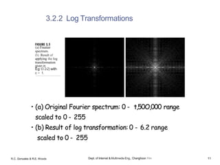
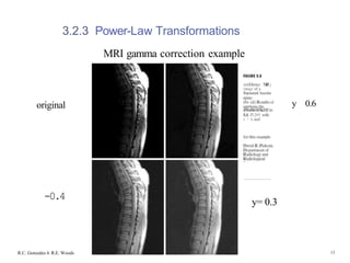
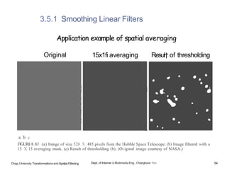
Chapter 3 discusses image enhancement techniques, focusing on spatial domain processing and intensity transformation functions. Key topics include histogram processing, point processing, log transformations, power-law transformations, and piecewise-linear transformation functions. The chapter emphasizes the direct manipulation of pixel values to improve image quality and highlight desired features.
![3.2.1 Image Negatives
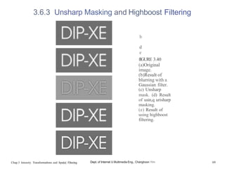
FMUB£3.9
(a)Original
digital
mammogram.
(b) Negative
iro•8e obtained
using the negative
transformation in
Eg. (ñ.2-I).
(CTourtesy of G.E.
Medical Systems.)
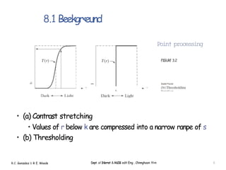
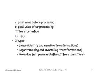
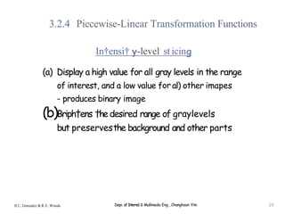
• Negative of an image with gray level [0, L-1]
s - L- 1 - r
• Enhancing whi†e or gray de†oil embedded in dark regions
of an image
R.C. Gonzales & R.E. Woods Dept. of Internet &Multimedia Eng., Changhoon Yim 9](https://image.slidesharecdn.com/dipunit3-240415144606-66a3cc29/85/Image-Enhancement-in-Spatial-Frequency-Domain-9-320.jpg)
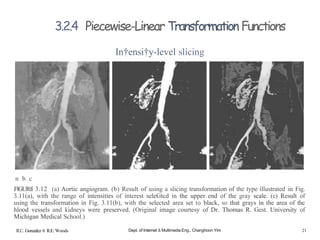
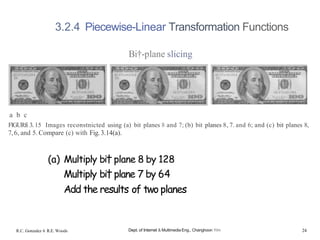
![3.2.4 Piecewise-Linear Transformation Functions
R.C. Gonzales & R.E. Woods
In†ensi†y-level slicing
1 —1 0
Dept. of Internet &Multimedia Eng., Changhoon Yim
FMURG B.I1
(a)this
highlights rangc
{A, B}of eray
levels and reduces
constant level.
transformation
highlights range
[ A, 8] t›tlt
preserres all
othor lovelx
(c) An image.
(d) Result of
u•ng‹he
19](https://image.slidesharecdn.com/dipunit3-240415144606-66a3cc29/85/Image-Enhancement-in-Spatial-Frequency-Domain-19-320.jpg)
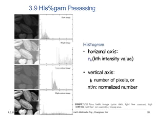
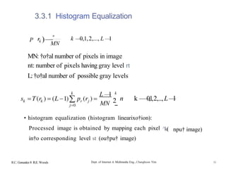
![• The histogram of digital image with gray levels in the
range [0, L-1] is a discrete function
• h(rk) k
rk: k†h 9••y level
nk:number of pixels in image having gray levels rt
• Normalized histogram
p(rk) °k °
n: †o†al number of pixels in image
n MN (M: row dimension, N: column dimension)
R.C. Gonzalez & R E. Woods Depi. of Interne1 & Mullimedia Eng , Changhoon Yim 25](https://image.slidesharecdn.com/dipunit3-240415144606-66a3cc29/85/Image-Enhancement-in-Spatial-Frequency-Domain-25-320.jpg)
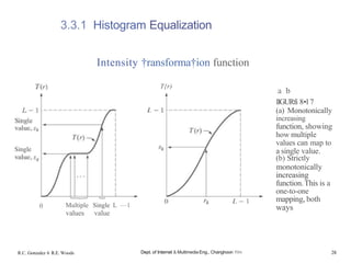
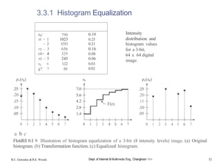
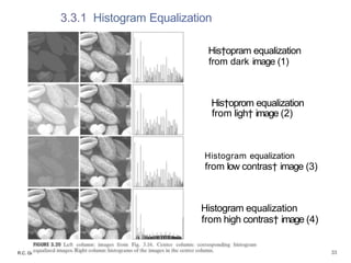
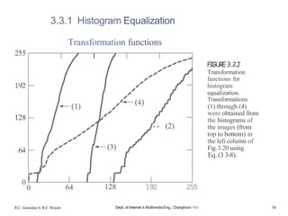
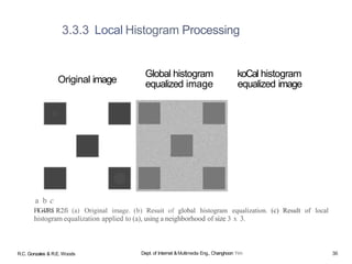
![3.3.1 Histogram Equalization
r: in†ensi†ies of †he image †o be enhanced
r is in †he range [0, L-1]
r 0: black, r L-1: whi†e
s: processed gray levels for every pixel value r
s= T(r), 0 ‹ r ‹ L
—
/
Requirements of †ransforma†ion function T
(a) T(r) is a (s†ric†Iy) mOnO†OniCaIly increasing in †he in†ervaI
0 :! r ‹ L
—
I
(b) 0 ‹ T(r) ‹ L-t for 0 ‹ r ‹ L-1
• Inverse transformation
r - T '(s), 0 ‹s ‹L-1
R.C. Gonzalez 8 R.E. Woods Depi. of Interne1 & Mullimedia Eng , Changhoon Yim 27](https://image.slidesharecdn.com/dipunit3-240415144606-66a3cc29/85/Image-Enhancement-in-Spatial-Frequency-Domain-27-320.jpg)
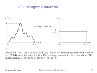
![3.3.1 Histogram Equalization
In†ensi†y leveis: random variable in in†ervai [0, L.-1]
dr
de
probabiii†y densi†y function (PDF)
.r = T r) = (L —1))(t pr(«)d+ cumula†ive dis†ribu†ion function (CDF)
d’ 'T $')
r d
{L ' ) d
' d r " ' ’ ” ( J
1
] = (L )Ür(r)
1
(L —1)p,.(r) L —
1 0 <s < L—
l
Uniforrn probabili†y densi†y function
R.C. Gonzalez & R E. Woods Depl. of Interne1 & Mullimedia Eng , Changhoon Yim 29](https://image.slidesharecdn.com/dipunit3-240415144606-66a3cc29/85/Image-Enhancement-in-Spatial-Frequency-Domain-29-320.jpg)
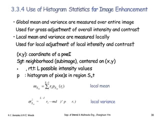
![3.3.4 Use ofHistogram Statistics for Image Enhancement
r: discre†e random variable represen†ing in†ensi†y values in †he range [0, L
—
1]
p(rá): normolized his†ogram componen† corresponding †o value rá
—rt/)" p(r,) nth momen† of r
c
—
i
r,per,)
i=0
›
Z •. —••2
p(ri)
i=0
m
/'2(r)
1
MN
R.C. Gonzalez 8 R.E. Woods
if —
I N—I
mean (average) value of r
Variance of r, 62(r)
M —
1 N —
l
MN Z L If •
sample mean
) —
m]2
sample variance
Dept. of Internet & Multimedia Eng., Changhoon Yim 37](https://image.slidesharecdn.com/dipunit3-240415144606-66a3cc29/85/Image-Enhancement-in-Spatial-Frequency-Domain-37-320.jpg)
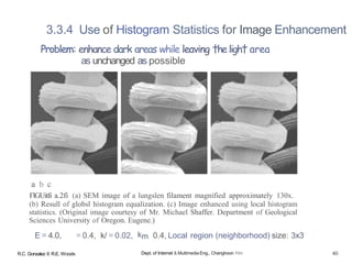
![3.3.4 Use of Histogram Statistics for Image Enhancement
• A measure whether an area is relatively liph† or dark a† (x,y)
Compare †he local average gray level ^*s †o the global mean md
(x,y) is a candidate for enhancement i* s ‹ ko s
• Enhance areas that have low contrast
Compare †he local standard deviation *s ,†o †he global standard
deviation 6G
(x,y) is a candidate for enhancemen† if bSt ‹ k
, 6G
• Res†ric† lowest values of contras†
(x,y) is a candidate for enhancemen† if k] 6c‹ 6s
• Enhancemen† is processed simply multiplying †he gray )evel
by acons†an† E
R.C. Gonzalez 8 R.E. Woods
s„
E J’{x, y) il
f{x, y)
c
ko AND i c —
< s„ —
<
otherwise
Depi. of Interne1 & Mullimedia Eng , Changhoon Yim 39](https://image.slidesharecdn.com/dipunit3-240415144606-66a3cc29/85/Image-Enhancement-in-Spatial-Frequency-Domain-39-320.jpg)
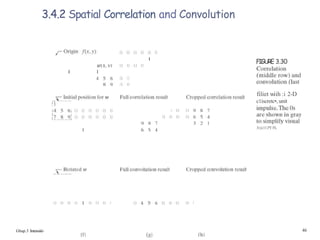
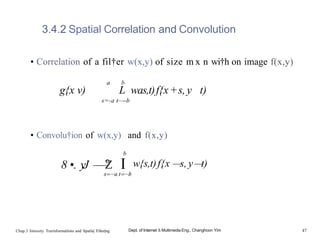
![3.4.2 Spatial Correlation and Convolution
(a) 0 0 0 1 0 0 0 0 1 2 3 2 8
1 2 3 2 8
Staztfng p«cIkm abgnmrnl
I 2 3 2 8
0 b 0 1 0 b 0 0 8 2 3 2 1 (i)
8 2 3 2 1
8 2 3 2 1
ta) 0 0 0 0 0 0 0 i 0 0 0 0 0 0 0 0 0 0 0 0 0 0 0 1 0 0 0 0 0 0 0 0 t1)
1 2 3 2 8 8 2 3 2 I
(¢) 0 0 0 0 0 0 0 I D 0 0 0 0 0 0 0 0 II II 0 ¢I II 0 ! 0 0 II 0 0 II ¢J 0 (ITI)
1 2 3 2 8 8 2 3 2 1
{I) 0 0 0 0 0 0 0 1 0 0 0 0 0 0 0 0 0 0 0 0 0 0 0 1 0 0 0 0 0 0 0 0 {n)
Fñ0 e l a t i o n rr•ili Full coovofuiio0 result
(g) 0 0 0 8 2 3 2 1 0 0 0 0 0 0 0 1 2 3 2 8 0 0 0 0 {o)
{h)
uAlM
0 6 ] J 2 1 U 0 0 1 2 3 2 b If 0
Fi I £ Illustmtioa of 1-Dcorrelation and tonvoluiion of a filter with a discrete unit impulse. hfote that
qp$ correlation rindconvolution are functions of &ip&cement.
qpyj](https://image.slidesharecdn.com/dipunit3-240415144606-66a3cc29/85/Image-Enhancement-in-Spatial-Frequency-Domain-45-320.jpg)
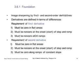
![3.6.1 Foundation
!f (x) = /(x +l) —/(x)
*f (x —
1) = f x) —]’ —
!)
firs†-order derivative
/(x +1)+ (A 1) —
2 (A) second-order derivo†ive
Ghap.3 Ir lensity Transformalions and Spatial Filtering Depl. of It41erne1 & Multimedia Eng., Changhoon Yiin 59](https://image.slidesharecdn.com/dipunit3-240415144606-66a3cc29/85/Image-Enhancement-in-Spatial-Frequency-Domain-59-320.jpg)
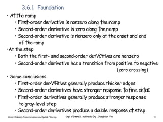
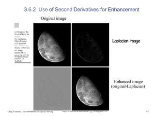
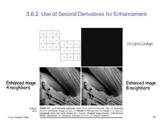
![3.6.2 Use of Second Derivatives for Enhancement
• Isotropic filters: ro†a†ion invorian†
• Simplex† isotropic second—order derivative opera†or‹ Laplacian
2-D Laplacian operation
—
—
f(x +1,y) f(x —
1,y) —
2f(•, ) x-direction
—
—f[x, y+ I) + J’(x, y —
1) —
2/’(x, y) y-direction
P2
f x, y)= [f x+1,y) f{x —
1,y) f{x, y+1)+ f{x, y —
1)]—
4 f{x, y)
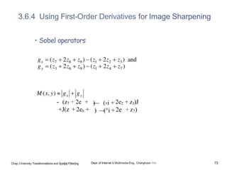
Chap.3 intensity Transformations and Spatial Filt6rin0 Dept. of Internet & Multimedia Eng., Changhoon Yim 62](https://image.slidesharecdn.com/dipunit3-240415144606-66a3cc29/85/Image-Enhancement-in-Spatial-Frequency-Domain-62-320.jpg)
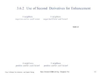
![3.6.2 Use ofSecond Derivatives for Enhancement
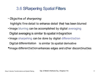
• Image enhancemen† (sharpening) by Laplacian operation
g(x, y) —
—
f{x, y) —92
f(x, y) if the center coefficient of the
Laplacian mask is negative
f{x, y)+ 02
f x, y) if the center coefficient of the
Laplacian mask is positive
SimpIÏfiCa†iOn
g(•. )= f(•. y)—[f(•+i,›)+ f •—i,v)+ f •. y+ )
+ f{x, y —
l)] + 4f(x, y)
—
—
5 f lx, y) —[f lx +1, y)+ f ‹x —
!, y1
+ f{x, y+ l)+ f{x, y —l))
Chap.3 intensité Transformations and Spatial Filt6ri€0 Dep. of Internet & Mullmedia Enq., Changhoon Yim 64](https://image.slidesharecdn.com/dipunit3-240415144606-66a3cc29/85/Image-Enhancement-in-Spatial-Frequency-Domain-64-320.jpg)