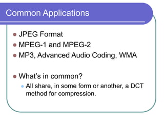
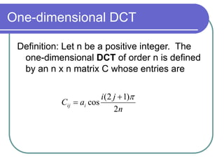
The document discusses the discrete cosine transform (DCT) and its applications in image compression. DCT transforms a signal or image into a combination of cosine functions arranged by frequency. This property allows for efficient compression by discarding high-frequency components with little visual impact. Specifically: - DCT provides a basis to represent an image as a sum of cosine functions, with low frequencies more important visually. 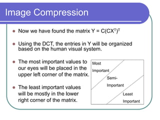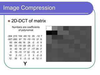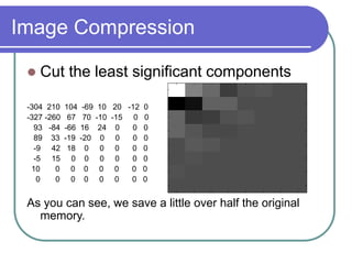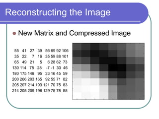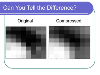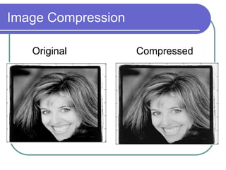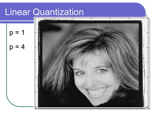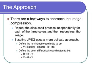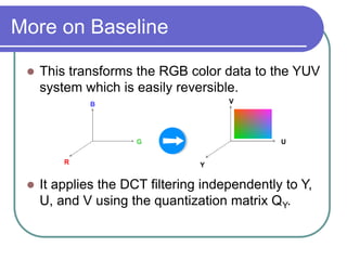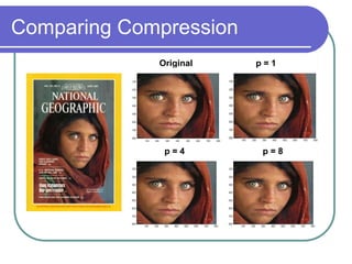- Applying DCT to blocks of an image separates information by importance, allowing lossy compression by discarding high frequencies. 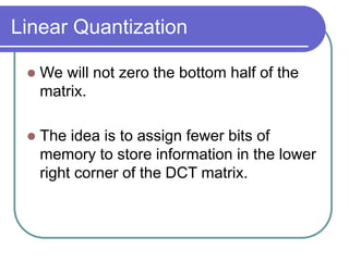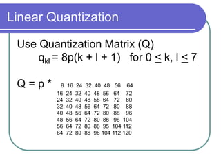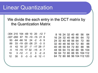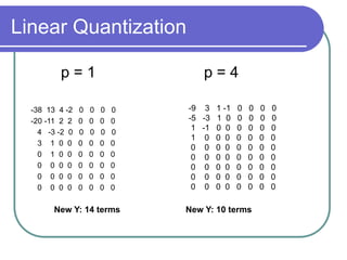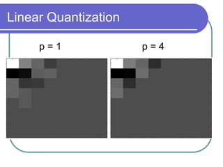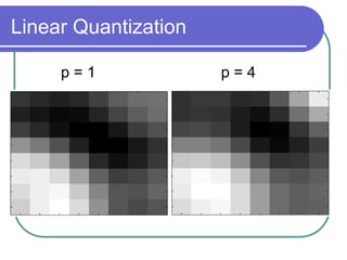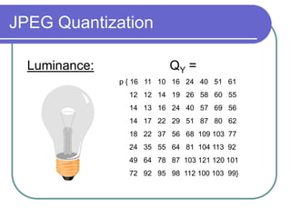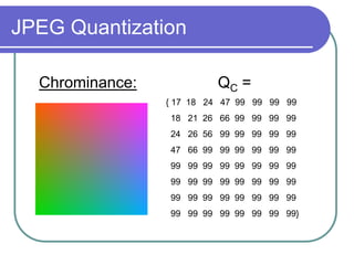- Quantization further compresses data by allocating fewer bits to store high-frequency DCT coefficients. - Together DCT and quantization provide significant data compression with minimal visual

1. Discrete Cosine Transform
and Image Compression
MTH/CSC 421
Thomas Buck Jimmie Maggard
Regal Ferrulli Zachary Hilty

2. Common Applications
 JPEG Format
 MPEG-1 and MPEG-2
 MP3, Advanced Audio Coding, WMA
 What’s in common?
 All share, in some form or another, a DCT
method for compression.

3. Overview
 One-dimensional DCT
 Least Squares Approximation
 Two-dimensional DCT
 Image Compression (grayscale, color)

4. One-dimensional DCT
Definition: Let n be a positive integer. The
one-dimensional DCT of order n is defined
by an n x n matrix C whose entries are
n
j
i
a
C i
ij
2
)
1
2
(
cos




5. The Advantage of Orthogonality
 C orthogonal: CTC = I
 Implies C-1 = CT
 Makes solving matrix equations easy
 Solve Y = CXCT for X:
 CTY = CTCXCY = XCT
 CTYC = XCTC = X

6. One-dimensional DCT
The discrete cosine transform, C, has one basic
characteristic: it is a real orthogonal matrix.
























n
n
n
n
n
n
n
n
n
n
n
n
C
2
)
1
2
)(
1
(
cos
2
3
)
1
(
cos
2
)
1
(
cos
2
)
1
2
(
cos
2
3
cos
2
cos
2
1
2
1
2
1
2







































n
n
n
n
n
n
n
n
n
n
n
n
C
C T
2
)
1
2
)(
1
(
cos
2
)
1
2
(
cos
2
1
2
3
)
1
(
cos
2
3
cos
2
1
2
)
1
(
cos
2
cos
2
1
2
1














7. One-dimensional DCT
 DCT Interpolation Theorem






1
1
0
2
)
1
2
(
cos
2
1
)
(
n
k
k
n
n
t
k
y
n
y
n
t
P

satisfies Pn(j)=xj for j=0,…, n-1
C transforms the n data points into n interpolation
coefficients. The DCT provides coefficients for
the trigonometric interpolation function using
only cosine terms.

8. One-dimensional DCT
Suppose we are given a vector
 T
n
y
y
y 1
0 ,
, 
 
 T
n
x
x
x 1
0 ,
, 
 
The Discrete Cosine Transform of x is the n-
dimensional vector
Where C is defined as
Cx
y 

9. Interpolation with DCT
 Why interpolate with DCT?
 What about Lagrange or Splines?
 DCT interpolation gives terms already
arranged in terms of importance to the human
visual system !!
 First terms are most important, last terms are
least important

10. One-dimensional DCT
 Least Squares Approximation Theorem
n
t
k
y
n
y
n
t
P
m
k
k
m
2
)
1
2
(
cos
2
1
)
(
1
1
0



 


 T
n
x
x
x 1
0 ,
, 
 
  Cx
y
y
y
T
n 
 1
0 ,
,

11. DCT Interpolation & Approximation
0 1 2 3 4 5 6 7 8
-7
-6
-5
-4
-3
-2
-1
0
1
2
0 1 2 3 4 5 6 7 8
-7
-6
-5
-4
-3
-2
-1
0
1
2

12. 2-D DCT Interpolation
1 1 1 1
1 0 0 1
1 0 0 1
1 1 1 1
Given a matrix of 16
data points we can plot
the surface in 3-D
space.

13. 2-D Least Squares
 Done in the same way as with 1-D
 Implement a low pass filter (drop terms)
 Delete the “high-frequency” components

14. 2-D Least Squares
1.25 0.75 0.75 1.25
0.75 0.25 0.25 0.75
0.75 0.25 0.25 0.75
1.25 0.75 0.75 1.25
Least Squares
Approximation
Sizeable Error due to small
number of points

15. Two-Dimensional DCT
 Idea 2D-DCT: Interpolate the data with a set
of basis functions
 Organize information by order of importance to
the human visual system
 Used to compress small blocks of an image
(8 x 8 pixels in our case)

16. Two-Dimensional DCT
Use One-Dimensional DCT in both
horizontal and vertical directions.
First direction F = C*XT
Second direction G = C*FT
We can say 2D-DCT is the matrix:
Y = C(CXT)T

17. Image Compression
 Image compression is a method that reduces the
amount of memory it takes to store in image.
 We will exploit the fact that the DCT matrix is based on
our visual system for the purpose of image
compression.
 This means we can delete the least significant values
without our eyes noticing the difference.

18. Image Compression
 Now we have found the matrix Y = C(CXT)T
 Using the DCT, the entries in Y will be organized
based on the human visual system.
 The most important values to
our eyes will be placed in the
upper left corner of the matrix.
 The least important values
will be mostly in the lower
right corner of the matrix.
Semi-
Important
Most
Important
Least
Important

19. Image Compression
8 x 8 Pixels Image

20. Image Compression
 Gray-Scale Example:
 Value Range 0 (black) --- 255 (white)
63 33 36 28 63 81 86 98
27 18 17 11 22 48 104 108
72 52 28 15 17 16 47 77
132 100 56 19 10 9 21 55
187 186 166 88 13 34 43 51
184 203 199 177 82 44 97 73
211 214 208 198 134 52 78 83
211 210 203 191 133 79 74 86
X

21. Image Compression
 2D-DCT of matrix
-304 210 104 -69 10 20 -12 7
-327 -260 67 70 -10 -15 21 8
93 -84 -66 16 24 -2 -5 9
89 33 -19 -20 -26 21 -3 0
-9 42 18 27 -7 -17 29 -7
-5 15 -10 17 32 -15 -4 7
10 3 -12 -1 2 3 -2 -3
12 30 0 -3 -3 -6 12 -1
Numbers are coefficients
of polynomial
Y

22. Image Compression
 Cut the least significant components
-304 210 104 -69 10 20 -12 0
-327 -260 67 70 -10 -15 0 0
93 -84 -66 16 24 0 0 0
89 33 -19 -20 0 0 0 0
-9 42 18 0 0 0 0 0
-5 15 0 0 0 0 0 0
10 0 0 0 0 0 0 0
0 0 0 0 0 0 0 0
As you can see, we save a little over half the original
memory.

23. Inverse 2D-DCT
2D-DCT gives us Y = C(CXT)T which can be
rewritten
Y = CXCT
Since C is an orthogonal we can solve for X
using the fact C-1 = CT
Therefore, X = CTYC

24. Reconstructing the Image
 In Mathematical terms:
 Let X = (xij) be a matrix of n2 real numbers
 Y = (ykl) be the 2D-DCT of X
 a0 = 1/sqrt(2) and ak = 1 for k > 0
 Then:

 Satisfies Pn(I,j) = xij for I, j=0,…,n-1
n
j
l
n
s
k
a
a
y
n
t
s
P
n
k
n
l
l
k
kl
n
2
)
1
2
(
cos
2
)
1
2
(
cos
2
)
,
(
1
0
1
0

 

 





25. Reconstructing the Image
 New Matrix and Compressed Image
55 41 27 39 56 69 92 106
35 22 7 16 35 59 88 101
65 49 21 5 6 28 62 73
130 114 75 28 -7 -1 33 46
180 175 148 95 33 16 45 59
200 206 203 165 92 55 71 82
205 207 214 193 121 70 75 83
214 205 209 196 129 75 78 85

26. Can You Tell the Difference?
Original Compressed

27. Image Compression
Original Compressed

28. Tan without Danger

29. Linear Quantization
 We will not zero the bottom half of the
matrix.
 The idea is to assign fewer bits of
memory to store information in the lower
right corner of the DCT matrix.

30. Linear Quantization
Use Quantization Matrix (Q)
qkl = 8p(k + l + 1) for 0 < k, l < 7
Q = p * 8 16 24 32 40 48 56 64
16 24 32 40 48 56 64 72
24 32 40 48 56 64 72 80
32 40 48 56 64 72 80 88
40 48 56 64 72 80 88 96
48 56 64 72 80 88 96 104
56 64 72 80 88 95 104 112
64 72 80 88 96 104 112 120

31. Linear Quantization
 p is called the loss parameter
 It acts like a “knob” to control compression
 The greater p is the more you compress
the image

32. Linear Quantization
We divide the each entry in the DCT matrix by
the Quantization Matrix
-304 210 104 -69 10 20 -12 7
-327 -260 67 70 -10 -15 21 8
93 -84 -66 16 24 -2 -5 9
89 33 -19 -20 -26 21 -3 0
-9 42 18 27 -7 -17 29 -7
-5 15 -10 17 32 -15 -4 7
10 3 -12 -1 2 3 -2 -3
12 30 0 -3 -3 -6 12 -1
8 16 24 32 40 48 56 64
16 24 32 40 48 56 64 72
24 32 40 48 56 64 72 80
32 40 48 56 64 72 80 88
40 48 56 64 72 80 88 96
48 56 64 72 80 88 96 104
56 64 72 80 88 95 104 112
64 72 80 88 96 104 112 120

33. Linear Quantization
p = 1 p = 4
-38 13 4 -2 0 0 0 0
-20 -11 2 2 0 0 0 0
4 -3 -2 0 0 0 0 0
3 1 0 0 0 0 0 0
0 1 0 0 0 0 0 0
0 0 0 0 0 0 0 0
0 0 0 0 0 0 0 0
0 0 0 0 0 0 0 0
-9 3 1 -1 0 0 0 0
-5 -3 1 0 0 0 0 0
1 -1 0 0 0 0 0 0
1 0 0 0 0 0 0 0
0 0 0 0 0 0 0 0
0 0 0 0 0 0 0 0
0 0 0 0 0 0 0 0
0 0 0 0 0 0 0 0
0 0 0 0 0 0 0 0
New Y: 14 terms New Y: 10 terms

34. Linear Quantization
p = 1 p = 4

35. Linear Quantization
p = 1 p = 4

36. Linear Quantization
p = 4
p = 1

37. Memory Storage
 The original image uses one byte (8 bits)
for each pixel. Therefore, the amount of
memory needed for each 8 x 8 block is:
 8 x (82) = 512 bits

38. Is This Worth the Work?
 The question that arises is “How much
memory does this save?”
p Total bits Bits/pixel
X 512 8
1 249 3.89
2 191 2.98
3 147 2.30
Linear Quantization

39. JPEG Imaging
 It is fairly easy to extend this application
to color images.
 These are expressed in the RGB color
system.
 Each pixel is assigned three integers for
each color intensity.

40. RGB Coordinates

41. The Approach
 There are a few ways to approach the image
compression.
 Repeat the discussed process independently for
each of the three colors and then reconstruct the
image.
 Baseline JPEG uses a more delicate approach.
 Define the luminance coordinate to be:
 Y = 0.299R + 0.587G + 0.114B
 Define the color differences coordinates to be:
 U = B – Y
 V = R – Y

42. More on Baseline
 This transforms the RGB color data to the YUV
system which is easily reversible.
 It applies the DCT filtering independently to Y,
U, and V using the quantization matrix QY.
B
G
R
V
U
Y

43. JPEG Quantization
QY =
p { 16 11 10 16 24 40 51 61
12 12 14 19 26 58 60 55
14 13 16 24 40 57 69 56
14 17 22 29 51 87 80 62
18 22 37 56 68 109 103 77
24 35 55 64 81 104 113 92
49 64 78 87 103 121 120 101
72 92 95 98 112 100 103 99}
Luminance:

44. JPEG Quantization
QC =
{ 17 18 24 47 99 99 99 99
18 21 26 66 99 99 99 99
24 26 56 99 99 99 99 99
47 66 99 99 99 99 99 99
99 99 99 99 99 99 99 99
99 99 99 99 99 99 99 99
99 99 99 99 99 99 99 99
99 99 99 99 99 99 99 99}
Chrominance:

45. Luminance and Chrominance
 Human eye is more sensible to luminance
(Y coordinate).
 It is less sensible to color changes
(UV coordinates).
 Then: compress more on UV !
 Consequence: color images are more compressible
than grayscale ones

46. Reconstitution
 After compression, Y, U, and V, are recombined and
converted back to RGB to form the compressed color
image:
B= U+Y
R= V+Y
G= (Y- 0.299R - 0.114B) / 0.587

47. Comparing Compression
Original p = 1
p = 4 p = 8

48. Up Close

49. The
End
Thanks for Coming!