Ifrs9 ntu mfe2000-ews-credit-deterioration

Implications for the new IFRS9 standards where the stage 2 or 3 designation is a
result of severe credit deterioration:
This study by my MSc students in 2000 suggests an empirical approach to identify
some KRIs or early warning signs of this type of credit deterioration, which can be
used as regime change indicators based on the IFRS9 reporting.
AN EMPIRICAL INVESTIGATION OF
A STRUCTURAL CREDIT RISK MODEL
Submitted by:
KOO WAI MING
LEE TECK KIANG
CAROLYN SIM BOON KHENG
Supervisor:
ASSOC PROF KHOO GUAN SENG

M.SC.(FINANCIAL ENGINEERING) DISSERTATION
Submitted in partial fulfilment of the requirements for
The degree of Master of Science (Financial Engineering)
in
Nanyang Technological University
(2000)

ACKNOWLEDGEMENTS
We would like to express our heartfelt thanks to our supervisor, Assoc Prof Khoo
Guan Seng, for his guidance, support and ideas throughout the preparation of this
dissertation. We are also deeply thankful to Mr Seow Kok Leong of the Monetary
Authority of Singapore for his considerable assistance during the data gathering
process of our research. Special thanks also goes to Mr Richard Teng of the
Monetary Authority of Singapore, and Ms Darrell Lam of the Singapore Exchange,
for being excellent information sources. We are also grateful to Dr Lawrence Ma of
Man-Drapeau Research for his invaluable insights, and Assoc Prof Ho Kim Wai for
his continuous support and encouragement. In addition, we thank the Monetary
Authority of Singapore and Man-Drapeau Research for providing financial support to
Carolyn and Teck Kiang respectively. Finally, we are appreciative of our families
who bore patiently the pressures caused by our commitment to complete this
dissertation. We are thankful for their understanding.

1
TABLE OF CONTENTS
Declaration
Acknowledgements
Table of Contents 1
Abstract 2
Chapter 1 Introduction 3
1.1 Overview 3
1.2 Motivation 5
1.3 Organization 6
Chapter 2 Background 7
2.1 Equity as call option 7
2.2 Calculation of EDF 9
2.3 Calculation of volatility 13
Chapter 3 Data 15
3.1 Selection of companies 15
3.2 Data collection 15
3.3 Data treatment 18
Chapter 4 Results and Discussion 20
4.1 Sensitivity Analysis 20
4.2 Financial Distress Prediction 26
4.3 Comparison of EDF with the Altman’s Z-score 31
Chapter 5 Conclusions 36
References 39

2
ABSTRACT
Default probabilities are important to the credit markets. Changes in default
probabilities of a borrowing firm may predict the occurrence of financial distress or
default in the firm. Knowing a firm’s default likelihood is important to financial
lenders as it allows them to estimate their resulting credit exposure to the firm. In this
dissertation, we examine the likelihood of default of a group of local companies listed
on the Singapore Exchange using the default prediction framework of the KMV
Corporation of San Francisco. Although a variety of default risk models are available
in the market, we have chosen the KMV approach for several reasons. First, it is
relatively simple to implement. Second, by being based on stock market data rather
than “historic” book value accounting data, it is forward-looking. Third, it has strong
theoretical underpinnings, having its basis on the modern theory of corporate finance
and options. Based on our study, there appears to be significant leading information
about credit events in the expected default frequencies (EDFs) generated using the
KMV framework. Typically, the EDFs are able to predict the occurrence of financial
distress about six months in advance. In some cases, the distress prediction horizon
can be as long as 18 months. To assess the performance of the KMV approach in
forecasting default likelihood, we compared its results with those produced by the
Altman’s Z-score model, a credit rating method based on accounting information.
Generally, both approaches yielded consistent results in the prediction of financial
distress. This suggests that a company’s equity price and volatility do contain up-to-
date information of its financial status and business risk.

3
Chapter 1
INTRODUCTION
1.1 Overview
Credit risk is the uncertainty faced by a lender or creditor due to the possibility that
the debtor may fail to honor its financial obligation. This failure results from the
occurrence of some “credit event”. There is no strict definition of what a credit event
is. It can include bankruptcy, downgrade, failure to pay, repudiation or restructuring.
Credit risk is dynamic and is related to market risk because credit risk changes with
variations in the value of the debtor’s assets. There are two basic components in
credit risk: default risk and recovery risk. Default risk is the possibility that the debtor
will fail to meet its obligations, and recovery risk is the possibility that the recovery
value of the defaulted contract may be less than its promised value.
This dissertation is primarily concerned with corporate default risk. From a
theoretical perspective, default risk has been modeled in a variety of ways. A first
approach, often referred to as the accounting approach undertaken by Edward Altman
(1968), uses financial ratios and discriminant analysis to assess a firm’s credit quality.
This approach yields ordinal groups which label firms by their financial health (e.g.
healthy, uncertain (grey), bankrupt). More information on this model will be
presented in Chapter 4.

4
A second approach has been to model default as a rare event, or Poisson process.
Mason and Bhattachayra (1981) allowed the firm’s default to follow a discontinuous
Poisson process with more complex boundary conditions. Jarrow and Turnbull
(1995) model default as a Poisson event when pricing derivatives with credit risk.
Duffie and Singleton (1996), when considering the term structure of defaultable bonds
or swaps, model the default event as an inaccessible stopping time, such as a Poisson
arrival. They argue that this is appropriate because when defaults do occur, they are
rarely anticipated even a short time before the event.
A third approach to default risk modeling is the option pricing theory analysis, first
applied to defaultable bonds by Merton (1974). Here, the payoff from a default risky
bond at maturity is seen as isomorphic to the payoff from an option, where the
underlying asset is the value of the firm. Specifically, the payoff to the bondholder at
maturity is the face value of the bond minus a put option on the firm’s value with an
exercise price equal to the face value of the bond. Using insights from option pricing
theory, Merton derived an explicit valuation formula for default-risky bonds that
default at maturity. The valuation formula requires knowing the following inputs : the
value of the firm, the face amount of the debt, the volatility of the firm’s value, the
yield on a default-free bond that matures at the same time, and the time to maturity of
the bond.
The classical Merton model has undergone many extensions over the past decade.
One example is the Credit Monitor Model of the KMV Corporation of San Francisco.
Under its approach, KMV views an equity holding as holding a call option whose

5
underlying is the firm’s assets with strike price equal to the firm’s liabilities. Using
the Black-Scholes option pricing formula and the theoretical relationship between the
volatilities of an option and its underlying asset, KMV then infers the market value
and volatility of the firm’s assets from market observable value and volatility of the
firm’s equity. These quantities are then employed, along with assumptions about the
firm’s debt level and time horizon of the debt, to derive the firm’s expected default
frequency (EDF), which is the likelihood of the firm defaulting on its loan within a
given time frame. A more detailed explanation of the KMV model will be presented
in Chapter 2.
1.2 Motivation
In this dissertation, we will apply the KMV default prediction framework to examine
the likelihood of default of local companies listed on the Singapore Exchange. We
have selected the KMV approach for research on local companies because of its
interesting features. First, it can be applied to any public company and relies on
publicly available information. Second, the model has strong theoretical
underpinnings as it is based on the modern theory of corporate finance and options,
where equity is viewed as a call option on the assets of a firm. Third, a basic tenet of
the model is that a borrowing firm’s stock price and volatility of its stock price
contain all information about the firm, including its financial health. Consequently, it
might be argued that the model might not work well in emerging markets, which are
less transparent than developed markets such as the US. It would thus be useful to
explore the applicability of the KMV framework to Singapore-listed companies.

6
However, unlike the KMV model which generates empirical EDFs based on historical
data of actual firm defaults, we shall construct theoretical EDFs based on the
assumption of normality of asset returns. In addition, because of data limitations and
the lack of proprietary information on the KMV model, we shall select the input
parameters for the model (such as the debt level and maturity of the debt) using
sensitivity analysis. We then compare how the model performs relative to an
accounting-based credit rating method, namely, the Altman’s Z-score model. To
facilitate our study, we have written numerical procedures using the MATLAB
software to invert the Black-Scholes equation and compute the EDF based on the
KMV approach.
1.3 Organization
The remainder of this thesis is organized as follows: Chapter 2 gives a background of
the KMV Credit Monitor Model, including an explanation of the mathematics behind
the model as well as the assumptions underlying the model. Chapter 3 describes our
data sources and a discussion of the data used in our analysis. Issues such as the
selection criteria and the treatment of data are discussed. Chapter 4 presents our
findings, paying particular attention to the sensitivity of the KMV methodology to
parameters related to the value of the borrowing firm, as well as the default prediction
capability of the approach in respect of local companies. Finally, Chapter 5 offers
some conclusions.

7
Chapter 2
BACKGROUND
In this chapter, the basic concepts behind the KMV Credit Monitor Model are
introduced. The mathematics involved in the calculation of the default probability
and volatility is also given. In addition, major differences between the actual KMV
model (Vasicek, 1984; Crosbie, 1999) and the adaptation used in this dissertation are
highlighted.
2.1 Equity as call option
The Credit Monitor Model developed by the KMV Corporation of San Francisco is
based on the model of a firm’s capital structure first proposed by Merton (1974).
Under this class of models, a firm is considered to be in default when the value of its
assets fall below that of it liabilities. The magnitude of the difference between the
assets and liabilities and the volatility of the assets, together with some suitable
assumptions about the distribution of the asset value, can then be used to determine
the borrower’s default probability.
To derive the market value of the firm’s assets and its volatility, which are not directly
observable, the KMV model makes use of the option nature of equity holding in a
leveraged firm. Suppose the market value of a firm’s assets is greater than the value
of its liabilities at the end of the loan period. The firm will repay its loans and the
equity holders will keep the residual value of the firm’s assets. The greater the value

8
of the assets, the greater the payoff to the equity holders. On the other hand, if the
value of the firm’s assets falls below the value of its liabilities, the equity holders will
prefer to turn the firm’s assets over to the lenders. The downside risk of the equity
holders is truncated no matter how low the asset value is, compared to the amount
borrowed. The payoff function, with limited downside and long-tailed upside, is
therefore similar to that of a call option. An equity holding can thus be viewed as
holding a call option whose underlying is the firm’s assets with a strike price equal to
the firm’s liabilities.
Default
point
Equity
payoff
Asset value
Figure 2.1 Payoff function of equity holding.
The stock can therefore be priced as an option on the assets of the firm using the
Black-Scholes option pricing formula. Together with the theoretical relationship
between the volatilities of an option and its underlying asset, the value of a firm’s
assets and its volatility can be calculated using market observable value and volatility
of the firm’s equity. With these, the KMV model calculates the distance-to-default,

9
which is the number of standard deviations that the firm is away from its default point
at the end of the loan period. From this, the expected default frequency (EDF) can be
derived by assuming a suitable asset value distribution at the end of the period.
Default
point
Asset
value
Possible asset
value path
EDF
DD
Figure 2.2 Expected default frequency and distance-to-default
2.2 Calculation of EDF
This section describes the method used to calculate the EDF based on KMV’s
methodology. Some simplifying assumptions over the KMV methodology have to be
made due to the lack of proprietary data and information.
Based on the Black-Scholes option pricing model, the market value of equity and the
market value of assets are related by
( ) ( )21 dXNedNVV rT
AE
−
−= (2.1)

10
where
T
Tr
X
V
d
A
AA
σ
σ






++





=
2
ln
1
Tdd Aσ−= 12
N(•) is the normal cumulative distribution function,
VA is the market value of the firm’s assets,
VE is the market value of the firm’s equity,
X is the default point at time T,
σA is the volatility of the firm’s asset, and
r is the risk free rate.
The default point X is the critical market value of assets below which the firm will
default. In general, firms do not default when their asset value reaches the book value
of their total liabilities. Many continue to service their debts given the long-term
nature of some of their liabilities. The default point generally lies somewhere
between the book value of current liabilities and total liabilities.
The equity and asset volatility are related by
A
E
A
A
E
A
E
A
E
V
V
V
V
V
V
σ
σσ
∆=






∂
∂
=
(2.2)
where

11
σE is the volatility of the firm’s equity, and
∆ is the hedge ratio N(d1).
The relationship linking equity and asset volatility given in eq. (2.2) holds only
instantaneously. Solving eqs. (2.1) and (2.2) simultaneously for VA and σA would at
best yield an approximate solution. A more complex iterative procedure (Ronn and
Verma, 1986) to solve for the asset volatility is as follows. The equity volatility is
computed from a time series of stock prices of appropriate length. Using eq. (2.2), an
initial guess of the asset volatility is obtained. Applying this value to eq. (2.1), we
generate a time series of asset values. Since eq. (2.1) is non-linear, the asset values
are also computed iteratively. The volatility of the resulting asset returns is used as
the input to the next iteration of the procedure that in turn determines a new series of
asset values and hence a new series of asset returns. The procedure continues in this
manner until it converges.
The asset value and volatility thus obtained are used to parameterize the stochastic
process assumed to be followed by the market value of the firm’s assets given by
dzVdtVdV AAAA σµ += (2.3)
where
µ is the drift rate of the firm’s asset value, and
z is a Wiener process.
At time T, the market value of the firm’s asset, T
AV , is given by

12
TTVV A
A
A
T
A εσ
σ
µ +







−+=
2
lnln
2
(2.4)
where
ε is a standard normal random variable.
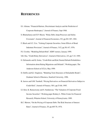
Eq. (2.4) involves estimation of the drift rate of the firm’s asset value which usually
involves significant error. KMV uses a constant drift rate for all firms in the same
market, which is the expected growth rate of the market as a whole. Based on the
same rational, the drift rate can be replaced by the risk free rate, which can be
estimated more accurately. We can then go on to calculate the upper bound of the
default probability assuming that the drift rate is always greater than the risk free rate.
The probability of default is the probability that the market value of the firm’s assets
will be less than the default point by the time the debt mature at time T. That is
[ ]
[ ]






















−+





−=














≥








−+





−=








≤+








−+=
≤=
≤=
T
Tr
X
V
N
T
Tr
X
V
P
XTTrVP
XVP
XVPEDF
A
AA
A
AA
A
A
A
T
A
T
A
σ
σ
ε
σ
σ
εσ
σ
2
ln
2
ln
ln
2
ln
lnln
2
2
2
(2.5)

13
where the distance-to-default
T
Tr
X
V
DD
A
AA
σ
σ








−+





=
2
ln
2
(2.6)
In the actual KMV model, instead of using the assumption of a normal distribution,
the distance-to-default is mapped to the EDF from a database with over 100,000
company-years of data with 2000 incidents of default or bankruptcy.
2.3 Calculation of volatility
The asset and equity volatilities are calculated from a time series of asset values and
closing stock prices. The continuously compounded asset and equity returns are first
calculated.






=
−1
ln
i
i
i
S
S
u (2.7)
where
ui is the asset or equity returns, and
Si is the asset value or closing stock price at period i.
The daily volatilities can then be estimated by the standard deviation of the return
series calculated using

14
( )∑=
−
−
=
n
i
i uu
n
s
1
2
1
1
(2.8)
where
u is the mean of ui’s.
This is then normalized to the annual volatilities by multiplying by the square root of
the approximate number of trading days per year.
252s=σ (2.9)
Since the KMV model is a forward looking model, a method that can forecast
volatility such as GARCH would in fact be more appropriate. However, in order not
to distract from the main objective of this study, the method that produces the
historical volatility is used.

15
Chapter 3
DATA
This chapter describes the criteria employed in the selection of companies used in this
study. Details of the collection and treatment of data are given provided.
3.1 Selection of companies
Companies selected in this study are, or were once, listed on the Singapore Exchange
or its predecessor, the Stock Exchange of Singapore. Since outright default cases are
rare, the study included companies that were in significant financial distress at some
point in time. By going through announcements filed with the stock exchange
between 1996 and 1999, 13 such companies were identified. There is no clear-cut
definition of what constitutes financial distress. Consequently, the severity of
financial distress varied among the companies selected. For example, Cam
International Holdings Limited, IPCO International Limited and Thakral Corporation
Limited were never in real default of their obligations. This, however, provided an
opportunity to study the efficacy of the model in identifying default or near-default
cases. The companies together with the announcement or event signifying financial
distress and the approximate date of financial distress are listed in Table 3.1.
3.2 Data collection
The default probabilities of the companies are followed for periods of 2 to 5 years up
to the approximate date of financial distress, depending on the availability of data.

16
Table 3.1 Companies selected for the study
Company Symbol Date Announcement / Event
Amcol Holdings Limited AMCO Jul 96 Went into default and was eventually
bought over.
Broadway Industrial Group
Limited
BRWY Jun 98 Announced that it was in negotiation with
its bankers to refinance existing borrowings
as well as potential investors to provide
additional funding.
Cam International Holdings
Limited (formerly Cam
Mechatronic Limited)
CAMT Jun 98 Company's auditors commented in its yearly
report that there were significant
uncertainties that might affect company's
ability to maintain or pay its debts as they
mature.
Form Holdings Limited FOHD Dec 98 Appointed Price Waterhouse as its financial
advisors to develop and implement a
restructuring plan.
GRP Limited GRPS Oct 98 Appointed KPMG as independent financial
advisors for purpose of loan restructuring.
IPC Corporation Limited IPCC Sep 98 Announced in its half-yearly financial
statement that its tight liquidity had resulted
in it being unable to meet certain of its
financial obligations.
IPCO International Limited IPCO Aug 97 HSBC Capital, the company's financier,
terminated a lease agreement and demanded
US$3.9m from company.
L & M Group Investments
Limited
LMGS Jun 99 Announced that it was negotiating to
refinance its outstanding loans from its
creditor banks.
Lim Kah Ngam Limited LKNS Jul 99 Started restructuring negotiations with its
creditor banks.
Pacific Can Investment
Holdings Limited
PCIS Apr 99 Announced its inability to repay its loan
stocks of $20m due.
Showpla Asia Limited SHOW Jun 98 Announced that it had been in discussion
with its bankers regarding the continuing
availability of its bank facilities.
Van der Horst Limited VDHS Jun 98 Announced that it was negotiating a
standstill agreement with its financial
lenders.
Thakral Corporation Limited THAK Jun 99 Announced that it was in technical breach
of certain financial convenants under its
facility agreement of US$250m.

17
The book value of liabilities is one of the inputs in the calculation of EDF. Yearly
data on the book value of liabilities are obtained directly from the annual reports of
the companies. Both the current and long term liabilities are collected to allow for the
study of the appropriate proportion of long-term liabilities to be included in
determining the default point.
The total market capitalization is another input in the calculation of EDF. Market
capitalization data are needed on a daily basis in order to calculate the volatility of
equity returns. Since these are not available directly from any source, they have to be
calculated by multiplying the daily stock price by the number of outstanding shares.
Stock price data are obtained from two separate sources due to the limitation of data
from both sources. For periods before 1997, the closing stock prices are obtained
from the Pacific-Basin Capital Markets (PACAP) database. For periods from 1997 to
1999, the closing stock prices are downloaded from Reuters 3000. Data from the two
sources are combined to produce a single time series of closing stock prices.
The number of outstanding ordinary shares is obtained from the companies’ annual
report. Where applicable, increase in the outstanding number of shares from year to
year and the reasons for the increase are noted in order to correctly interpolate the
numbers to a daily series to calculate the daily total market capitalization.

18
The final input in the calculation of EDF is the risk free interest rate. In this case, the
Singapore overnight lending rate is used. Weekly averages of the overnight rate are
downloaded from the Monetary Authority of Singapore web site.
Additional financial data are needed to calculate Altman’s Z-score which will be used
to compare with the EDF calculated. These include the working capital, total assets,
retained earnings, EBIT and sales. These data are similarly obtained from the balance
sheets and income statements in the companies’ annual reports.
With the exception of the number of outstanding shares, information in the annual
reports become available to the public only after their release, which is typically 3
months after the reporting date or end of financial year. Accordingly, data obtained
from the financial statements are dated by the release date of the reports and not the
reporting date.
3.3 Data treatment
Interpolation of data is necessary because it is desirable to study the default
probabilities from month to month while data from financial statements are only
available annually. Except for the number of outstanding ordinary shares, all other
data obtained from financial statements are assumed to be constant between the
release of annual reports.
Changes in the number of outstanding shares are commonly due to the issuance of
new shares, the issuance of bonus shares and the conversion of warrants. When the

19
main reason for the increase is due to the issuance of new or bonus shares, the number
of outstanding shares is taken to have changed instantaneously at the date of issuance.
When the main reason for the increase is due to the conversion of warrants, then the
increase is assumed to have taken place gradually over the period between the
reporting dates. In this case, the number of outstanding shares in between the
reporting dates are obtained by linear interpolation.
For the companies IPCO International Limited, Showpla Asia Limited and Thakral
Corporation Limited, the shares are quoted in US dollars but the financial statements
are in Singapore dollars. To reconcile the two, the share prices are converted to
Singapore dollars. The exchange rates are downloaded from Reuters 3000.

20
Chapter 4
RESULTS AND DISCUSSION
In this chapter, we present and analyze the EDFs estimated for the group of local
companies in our sample based on the KMV methodology. As a first step, we carried
out a systematic sensitivity analysis of the KMV approach to determine the effect of
the values of the input parameters, such as the debt level and maturity, on the EDF.
For companies that have encountered difficulties in honoring their financial
obligations, our analysis will focus on the assets values, asset volatility and EDF for
the year immediately preceding the date they went into financial distress. In addition,
the performance of the EDF in forecasting default likelihood will be compared with
the Altman’s Z-score, a credit rating index based on accounting information.
4.1 Sensitivity Analysis
As pointed out earlier, the chief obstacle to empirical application of the KMV
methodology in estimating default risk lies in the fact that neither the market value of
the firm, VA, nor its instantaneous volatility, σA, are directly observable. They have to
be deduced from the Black-Scholes equation using the firm’s market capitalization,
equity volatility, debt level and maturity, together with the assumption that the firm
has a single debt and that no financial restructuring occurs before the asset level falls
below the debt level. Obviously, these assumptions hardly hold in actual applications;
generalization of the KMV approach to handle more complex liability debt structure
and the possibility of financial restructuring has to be considered (Black and Cox,

21
1976; Das, 1995; Kim, Ramaswamy and Sundaresan, 1989; Nielson, Saa-Requejo and
Santa Clara, 1993; Shimko, Tejima and van Deventer, 1993). For this study, we
approximate the firm’s complex debt structure using a single effective debt level, B,
which is equal to the short-term debt plus a fraction, f, of the long-term debt, maturing
at a time, T, which could range from one to two years depending on the distribution of
the firm’s long and short-term debts. In effect, the single maturity, T, of the effective
liability plays a role similar to the duration in approximating the effective maturity of
a coupon bond. In addition, financial lenders of firms do not, as a first resort, step in
to liquidate a firm when the net worth of the firm has fully eroded. Rather, depending
on the bankruptcy codes and business environment, they may have the incentive to try
to revive the firm concerned through debt restructuring. Indeed, with the exception of
Amcol Holdings Limited (AMCO), the companies that we have selected in this study
have undergone some form of restructuring to resolve their financial difficulties. It is
therefore reasonable to assume that there is a hypothetical limit for the effective debt
level above which erosions in value, should they occur, would make the revival
efforts excessively costly, and below which financial lenders have the incentive to
restructure the debt. Expressing this hypothetical limit as a fraction, ρ (≤ 1), of the
effective debt, the value ρB will be the relevant debt level for the determination of the
firm’s asset level and volatility. With these assumptions, we continue to employ the
KMV approach to deduce the firm’s asset value and volatility, although the actual
values of the following three parameters, namely the fraction of long-term debt, f, its
effective maturity, T, and the fraction, ρ, will have to be estimated from past histories
of failure, or near-failure. It is conceivable that they will not be universal and will
vary from industry to industry. However, sensitivity analysis of the EDF can be

22
carried out to determine to what extent these parameters would affect the outcome of
the model.
Using the MATLAB program that has been written to invert the Black-Scholes
equation and compute the EDF, we generated monthly time-series of the EDF for
different values of f, T and ρ. The instantaneous equity volatilities required for this
purpose were computed using the preceding 90-day equity values. It is noted that the
EDFs computed do not differ significantly from those based on volatilities calculated
with longer time horizon. For illustrative purpose, we only display results for
Broadway Industrial Group Limited (BRWY), which went into financial distress in
June 1998. In figure 4.1, we plotted the EDF time series computed with T = 1 (i.e.
one year maturity for the effective debt), ρ = 1, and fraction of the long-term debt, f,
that ranges from 0 to 1 in steps of 0.2. These series of EDF plots illustrate what is
expected from the KMV methodology, namely an increase in the debt level increases
the likelihood of default. However, the magnitude of the variation in the EDF for
different f values is not uniform along the time horizon. In particular, for the case of
BRWY, for certain period of time, the EDF varies from 0.01 to 0.1 depending on the
fraction of long-term debt used. To put things in perspective, an EDF of 0.014 is
approximately equal to the annual default frequency of a BB rated bond in Moody’s
rating while an EDF of 0.1 is equivalent to a CCC bond in terms of annual default
frequency. For other periods of time, the variation is, however, not significant. We
also observed similar property for other companies in our sample. Nevertheless, we
notice that the choice of f, in all the cases that we have considered, does not affect the
performance of our approach in predicting the occurrence of financial distress in a

23
firm. Thus for subsequent analysis, we take f to be 0.2 uniformly across different
companies. It should be emphasized that for bond rating and valuation, which we do
not consider in this study, the choice of f will be important.
0.00001
0.0001
0.001
0.01
0.1
1
M
ar-95
Jun-95
Sep-95
Dec-95
M
ar-96
Jun-96
Sep-96
D
ec-96
M
ar-97
Jun-97
Sep-97
Dec-97
M
ar-98
Jun-98
f = 1.0
f = 0.8
f = 0.6
f = 0.4
f = 0.2
f = 0.0
Figure 4.1 EDFs for f ranging from 0.0 to 1.0.
Next we consider the effect of varying the parameter ρ on the EDF with the debt
maturity fixed at T = 1 and f = 0.2. Using BRWY as an example, we plotted in figure
4.2 the series of the EDF for ρ that takes values equal to 90%, 95% and 100%. As in
the previous case, the default likelihood increases with the fraction ρ since higher
fraction implies higher effective debt level. For all the companies that we have
considered, the EDF, as in the case of Broadway, does not vary significantly for
different ρ values. This is especially the case for the one-year period prior to the date
in financial distress. This finding shows that the possibility of financial restructuring

24
occurring before default has no significant impact on the prediction outcome.
Therefore, for subsequent analysis, we shall take ρ to be 100%.
0.00001
0.0001
0.001
0.01
0.1
1
M
ar-95
Jun-95
Sep-95
D
ec-95
M
ar-96
Jun-96
Sep-96
D
ec-96
M
ar-97
Jun-97
Sep-97
Dec-97
M
ar-98
Jun-98
ρ = 1.00
ρ = 0.95
ρ = 0.90
Figure 4.2 EDFs for ρ equal to 90%, 95%, and 100%.
To evaluate the effect of the effective debt’s maturity, T, on the default risk
prediction, we took ρ = 100% and f = 0.2 and generated series of EDF for T equal to
1, 1.5 and 2 years. The result for BRWY is plotted in figure 4.3 as an illustration. As
can be seen from the figure, EDF computed with longer maturity is higher than that
with shorter maturity. Nonetheless, for the few months immediately preceding the
financial distress, the three series of EDF exhibit increasing trends with little
difference in values. As we are mainly interested in the year immediately preceding
the financial distress date, and since our analysis shows that the choice of T does not
affect the EDF significantly, we select one year as the maturity of the effective debt
level for all the companies in our sample for subsequent computation. The choice of

25
T = 1 is reasonable since the effective debt is made up of all the short-term debts,
which have maturities shorter than one year, and 20% of the long-term debts, which
mature after one year.
0.00001
0.0001
0.001
0.01
0.1
1
M
ar-95
Jun-95
Sep-95
D
ec-95
M
ar-96
Jun-96
Sep-96
Dec-96
M
ar-97
Jun-97
Sep-97
D
ec-97
M
ar-98
Jun-98
T = 1.0
T = 1.5
T = 2.0
Figure 4.3 EDFs for T equal to 1.0, 1.5 and 2.0.
In summary, our sensitivity analysis shows that the EDFs computed with the different
values of T, f and ρ that we have considered, exhibit the same general feature across
the time horizon especially for the one-year period prior to the financial distress date.
This observation is consistent with the fact that close to the date of financial distress,
where the effective debt level of most of these companies are well below the market
values of their assets, Black-Scholes equation is not sensitive to minute change in the
input parameters. As we are essentially interested in investigating the ability of the
KMV approach in predicting financial distress, it is reasonable to fix these variables at
the appropriate values that we have chosen, namely f = 0.2, ρ = 1 and T = 1.

26
4.2 Financial Distress Prediction
With the selected T, f, ρ parameters’ values, we computed the EDF of the ten
companies that have encountered financial distress in our sample. Their EDFs are
plotted in figures 4.4 to 4.7, where the horizontal axis denotes the time horizon in
months before the date they went into financial distress. Except for AMCO, the levels
of their EDFs are sloping upward, toward progressively higher default likelihood, as
their distress dates drew closer, showing that EDFs computed based on the KMV
approach are consistent with the financial status of the companies. Using an EDF of
0.2, which is well above the annual default rate of a CCC bond in S&P and Moody’s
rating, as an indication of default, we observed that typically the EDF is able to
predict the occurrence of financial difficulty six months in advance. In fact in most
cases, such as Lim Kah Ngam Limited (LKNS) and Pacific Can Investment Holdings
Limited (PCIS), the distress prediction horizon is even longer. We also computed the
EDFs of three companies, namely Cam International Holdings Limited (CAMT),
IPCO International Limited (IPCO) and Thakral Corporation Limited (THAK), whose
financial problems are much less severe compared to the rest of companies in our
sample, as a consistency check of the KMV methodology. Their EDFs, which are
plotted in figure 4.8, are indeed below 0.2, the EDF level that we have selected to
indicate default.
For the case of AMCO, the EDFs computed are below 0.001 and there is no clear sign
of an increasing trend that indicate deterioration in the financial health of the
company. It is noted that the company’s share price in the period 1993 to 1995 (i.e.
the period prior to default) did not reflect the financial deterioration of the company.

27
At the beginning of 1993, the company’s share price started increasing rapidly,
reaching a peak of $4.90 on 10 Jan 94. The price continued to increase throughout
1994 and 1995. A possible reason for this could be the lack of information disclosure
on the part of the company. Consequently, the KMV approach that we have adopted
failed to capture the occurrence of financial distress in the company.
0.00001
0.0001
0.001
0.01
0.1
1
0123456789101112131415161718192021222324
Months before financial distress
BRWY
GRPS
FOHD
Figure 4.4 EDFs of BRWY, FOHD and GRPS.

28
0.00001
0.0001
0.001
0.01
0.1
1
0123456789101112131415161718192021222324
IPCC
LMGS
LKNS
Figure 4.5 EDFs of IPCC, LMGS and LKNS.
0.00001
0.0001
0.001
0.01
0.1
1
0123456789101112131415161718192021222324
PCIS
SHOW
VDHS
Figure 4.6 EDFs of PCIS, SHOW and VDHS.

29
1E-10
1E-09
1E-08
1E-07
1E-06
1E-05
0.0001
0.001
0.01
0.1
1
0123456789101112131415161718192021222324
AMCO
Figure 4.7 EDF of AMCO.
1E-10
1E-09
1E-08
1E-07
1E-06
1E-05
0.0001
0.001
0.01
0.1
1
0123456789101112131415161718192021222324
CAMT
IPCO
THAK
Figure 4.8 EDFs of companies with less severe financial problems.

30
It is also instructive and interesting to present the relationship between the firm’s
leverage and EDF in the context of the KMV methodology. In figure 4.9 and 4.10,
we display the effective debt, asset, and market capitalization of AMCO and BRWY
respectively. It is apparent from these two figures that asset value varies in tandem
with the market capitalization of the firms, in response to investors anticipation of the
firms’ future cash flows. This contrasts markedly with the debt level estimated from
the financial statement, which is inherently backward looking. For the case of
Broadway, as the financial difficulty drew nearer, the firm’s financial status is
reflected, through the company’s equity, in the market capitalization, that showed a
downward trend that eventually dipped below the firm’s liability. While for the case
of AMCO, it is intriguing that the market seems to be unaware of the imminent
financial crisis faced by the company given that the Altman’s Z-score, which we will
discuss in the next section, is able indicate the weak financial status of the company in
advance.
0
40,000
80,000
120,000
M
ar-95
Jun-95
Sep-95
D
ec-95
M
ar-96
Jun-96
Sep-96
Dec-96
M
ar-97
Jun-97
Sep-97
D
ec-97
M
ar-98
Jun-98
$'000
Debt
Asset
Market cap
Figure 4.9 Market capitalization, asset and debt of AMCO.

31
0
400,000
800,000
1,200,000
1,600,000
2,000,000
M
ar-91Jun-91Sep-91D
ec-91M
ar-92Jun-92Sep-92D
ec-92M
ar-93Jun-93Sep-93D
ec-93M
ar-94Jun-94Sep-94D
ec-94M
ar-95Jun-95Sep-95Dec-95M
ar-96Jun-96
$'000
Asset
Market Cap
Debt
Figure 4.10 Market capitalization, asset and debt BRWY.
4.3 Comparison of EDF with the Altman’s Z-score
Developed by E. I. Altman in 1968, the Altman’s Z-score is one of the best-known
bankruptcy prediction models. The model measures the financial health of a company
using several key accounting ratios that may indicate the potential for bankruptcy as
much as six months in advance. The Z-score has the form:
54321 999.06.03.34.12.1 XXXXXZ ++++= (4.1)
where
assetsTotal
capitalWorking
1 =X
assetsTotal
earningsRetained
2 =X

32
assetsTotal
EBIT
3 =X
sliabilitieofBook value
equityofueMarket val
4 =X
assetsTotal
Sales
5 =X
Using this methodology, a company would be categorized as “healthy” if it received a
score of 2.99 or above, “bankrupt” if the score was below 1.81 and “grey (or
uncertain)” if the score fell between these two points.
The Altman’s model differs in many ways from the KMV model; the former is
founded on accounting information that are deemed relevant to the financial health of
a company while the latter is rooted in modern asset pricing theory and relies largely
on market information of the firm. It would therefore be interesting to compare the
default prediction performance of these two different approaches. However, as the Z-
score does not translate directly into a probability of default, care must be taken in
comparing it with the EDF. Since a Z-score of 1.81 is considered default, we map it
to an EDF equal to 0.2, which is well above the annual default rate of the lowest CCC
grade bond rated by both S&P and Moody. Using these benchmarks, we then
determine the default prediction horizon (in months) of the two models. The results,
which are presented in the table below, shows that, except for the case of AMCO, the
Altman’s Z-score and EDF are able to consistently predict the upcoming distress at
least six months in advance. Unlike the EDF, the Z-score of AMCO, which is plotted
in figure 4.14, nonetheless indicates gradual decline in the financial well being of the
company for the years preceding default. Similarly for the rest of the companies in

33
our sample that have encountered distress, their Z-scores, as shown in figures 4.11 to
4.13, showed a decreasing trend that dropped below 1.81 prior to the default dates.
Table 4.1 Default prediction horizon (in months) of Z-score and EDF.
Company Z-score EDF
BRWY 11 7
FOHD > 10 > 10
GRPS 12 12
IPCC 6 6
LKNS 37 10
LMGS 14 19
PCIS 29 17
SHOW 9 11
VDHS 7 7
0
1
2
3
4
5
6
7
8
051015202530354045
BRWY
GRPS
FOHD
Figure 4.11 Z-scores of BRWY, FOHD and GRPS.

34
0
1
2
3
4
5
6
7
8
051015202530354045505560
LKNS
LMGS
IPCC
Figure 4.12 Z-scores of IPCC, LMGS and LKNS.
0
1
2
3
4
5
6
7
8
051015202530354045505560
VDHS
PCIS
SHOW
Figure 4.13 Z-scores of PCIS, SHOW and VDHS.

35
0
1
2
3
4
5
6
7
8
051015202530354045505560
AMCO
Figure 4.14 Z-score of AMCO.
Despite the simplification of the debt structure, the use of prior year’s financial
liabilities and the lognormal distribution assumed in the computation of the EDF, the
distress prediction capability of the EDF is almost on par with the Altman’s Z-score,
which relies on more inputs from the companies’ financial reports. This suggests that
a company’s equity price and volatility do contain up-to-date information of its
financial status and business risk. We expect, with more frequent updates on the
liabilities of the firm and a more careful treatment to incorporate the different
maturities and seniorities of the liabilities, the KMV’s approach in default risk
modeling will produce significantly better results.

36
Chapter 5
CONCLUSIONS
We have applied the KMV default prediction framework to examine the likelihood of
default of a group of local companies listed on the Singapore Exchange. These
companies were selected based on information that they were in significant financial
distress at some point in time.
In the absence of historical default statistics on local companies, we have assumed
that asset returns follow a normal distribution. In addition, due to the lack of
proprietary information on the KMV model, we have made some modifications to the
input parameters of the model. Our approach uses the following four-step process to
calculate the EDF:
1. Estimate the appropriate input parameters for the model using sensitivity
analysis;
2. Deduce the market value and volatility of the firm’s assets using observed
value and volatility of the firm’s equity and the input parameters estimated in
step 1;
3. Calculate the distance-to-default, the number of standard deviations the firm is
away from default; and
4. Derive the EDF by assuming that asset returns follow a normal distribution.

37
Our findings suggest that we can use a single effective debt level equivalent to the
short-term debt (i.e. those liabilities due within one year) plus a fraction of the long-
term debt as a reasonable approximation of a firm’s debt structure. For the purpose of
our study, we have fixed the proportion of long-term debt to be included in the
effective liability as 20%, and the maturity of the effective debt as one year. Our
results also indicate that the possibility of financial restructuring occurring prior to
default has no significant impact on the outcome of the model in the prediction of
financial distress.
We have also examined the EDFs before the event of a financial distress or default.
There appears to be significant leading information about the occurrence of financial
distress and about defaults in these forward looking EDFs generated using our
modified KMV approach. Except for one company, namely, Amcol Holdings
Limited, the level of EDF for the companies in our sample increased as the date on
which the companies went into financial distress drew near. We also observe that
typically, the EDF is able to predict the occurrence of financial difficulty about six
months in advance. In fact, in some cases, the distress prediction horizon can be as
long as 18 months. For the case of Amcol, our modified KMV approach failed to
capture the occurrence of financial distress chiefly because the company’s share price
for the period prior to default did not reflect its financial deterioration. One possible
reason for this could be the lack of information disclosure on the part of the company.
We have also compared the performance of our modified KMV model with an
accounting-based credit rating method, namely, the Altman’s Z-score model. It is

38
found that except for the case of Amcol, both models produce consistent results in the
prediction of financial distress in the companies we selected. In the case of Amcol,
Altman’s Z-score model outperformed our approach as it had predicted a deterioration
in the financial health of the company for the year prior to default.
While our modified KMV approach is generally able to predict the occurrence of
financial distress in local companies about one year ahead, it may not work well for
longer-term prediction horizons. Our approach also suffers from several drawbacks.
First, it assumes that asset returns are normally distributed. However, in practice, the
distribution of asset values is difficult to measure. Therefore, a question arises as to
whether it is reasonable to use the usual assumption of normal or lognormal
distributions. Second, our study has shown that the magnitude of variation in the
EDFs is sensitive to the parameters selected. Since our model uses one-size-fit-all
parameters, it cannot be used to price defaultable bonds. Moreover, the recovery rate,
an important factor in pricing defaultable bonds, is not determinable from the model.
One way in which our present approach can be refined to better capture a firm’s debt
level is to use Macaulay duration to reposition the face value of a firm’s multiple
liabilities to a single duration for all the liabilities (Delianedis and Geske, 1999).
However, we are not certain if this would actually improve the performance of the
model. Further empirical studies would need to be conducted to verify this.

39
REFERENCES
E.I. Altman, “Financial Rations, Discriminant Analysis and the Prediction of
Corporate Bankruptcy”, Journal of Finance, Sept 1968.
S. Bhattacharya and S.P. Mason, “Risky Debt, Jump Processes and Safety
Covenants”, Journal of Financial Economics, 9/3, pp.281-307, 1981.
F. Black and J.C. Cox, “Valuing Corporate Securities: Some Effects of Bond
Indenture Provisions”, Journal of Finance, 31/2, pp.361-67, 1976.
P.J. Crosbie, “Modeling Default Risk”, KMV memeo, January 1999.
S.R. Das, “Credit Risky Derivatives”, Journal of Derivatives, 2/3, pp.7-23, 1995.
G. Delianedis and R. Geske, “Credit Risk and Risk Neutral Default Probabilities:
Information about Rating Migrations and Defaults”, Working paper, The
Anderson School at UCLA, May 1999.
D. Duffie and K.J. Singleton, “Modeling Term Structures of Defaultable Bonds”,
Graduate School of Business, Stanford University, 1996.
R. Jarrow and S.M. Turnbull, “Pricing Derivatives on Financial Derivatives Subject to
Credit Risk”, Journal of Finance, 50/1, pp.53-86, 1995.
I.J. Kim, K. Ramaswamy and S. Sundaresan, “The Valuation of Corporate Fixed
Income Securities”, Working paper Rodney L. White Center for Financial
Research, Wharton School, University of Pennsylvania, 1989.
R.C. Merton, “On the Pricing of Corporate Debt: The Risk Structure of Interest
Rates”, Journal of Finance, 29, pp.449-70, 1974.

40
L.T. Nielson, J. Saa-Requejo and P. Santa Clara, “Default Risk and Interest Rate
Risk: The Term Structure of Default Spreads”, Working paper, INSEAD
Fontainebleau, France, 1993.
E.I. Ronn and K. Verma, “Pricing Risk-adjusted Deposit Insurance: An Option-Based
Model”, Journal of Finance, 41, pp.871-895, 1986.
D.N. Shimko, N. Tejima and D. van Deventer, “The Pricing of Risky Debt when
Interest Rates are Stochastic”, Journal of Fixed Income, 3, pp.58-65, 1993.
O.A. Vasicek, “Credit Valuation”, KMV memeo, March 1984.

Ifrs9 ntu mfe2000-ews-credit-deterioration

More Related Content

What's hot

Similar to Ifrs9 ntu mfe2000-ews-credit-deterioration

More from Guan Khoo

Recently uploaded

Ifrs9 ntu mfe2000-ews-credit-deterioration