Download to read offline
![M. Malik, L.C. Thomas / International Journal of Forecasting 28 (2012) 261–272 263
the loan (Section 7). Section 8 describes the full model
used, while Section 9 reports the results of out-of-sample
forecasts, and out-of-time and out-of-sample forecasts,
using the model. The final section draws some conclusions,
including how the model could be used. It also identifies
one issue — which economic variables drive consumer
credit risk — where further investigation would benefit all
models of consumer credit risk.
2. Behaviour score dynamics and Markov chain models
Consumer lenders use behavioural scores updated
every month to assess the credit risk of individual
borrowers. The score is considered to be a sufficient
indication of the probability that a borrower will be ‘‘Bad’’,
and so default within a certain time horizon (normally
taken to be the next twelve months). Borrowers who are
not Bad are classified as ‘‘Good’’. Thus, at time t, a typical
borrower with characteristics x(t) (which may describe
the recent repayment and usage performance, the current
information available on the borrower at a credit bureau,
and socio-demographic details) has a score s(x(t), t), so
p(B|x(t), t) = p(B|s(x(t), t)). (1)
Some lenders obtain a Probability of Default (PD), as
required under the Basel Accord, by taking a combination
of behavioural and application scores. New borrowers are
scored using only the application score to estimate PD, then
once there is sufficient history for a behavioural score to
be calculated, a weighted combination of the two scores
is used to calculate PD; eventually, the loan is sufficiently
mature that only the behavioural score is used to calculate
PD. The models described hereafter can also be applied to
such a combined scoring system.
Most scores are log odds score (Thomas, 2009a), and
thus the direct relationship between the score and the
probability of being Bad is given by
s(x(t), t) = log
P(G|s(x(t), t))
P(B|s(x(t), t))
⇔ P(B|s(x(t), t))
=
1
1 + es(x(t),t)
, (2)
though in reality this may not hold exactly. Applying the
Bayes theorem to Eq. (2) gives the expansion where if pG(t)
is the proportion of the population who are Good at time t
(pB(t) is the proportion who are Bad), one has
s(x(t), t) = log
P(G|s(x(t), t))
P(B|s(x(t), t))
= log
pG(t)
pB(t)
+ log
P(s(x(t), t)|G, t)
P(s(x(t), t)|B, t)
= spop(t) + woet (s(x(t), t)). (3)
The first term is the log of the population odds at time t
and the second term is the weight of evidence for that score
(Thomas, 2009a). This decomposition may not hold exactly
in practice, and is likely to change as a scorecard ages.
However, it shows that the term spop(t), which is common
to the scores of all borrowers, can be thought to play the
role of a systemic factor which affects the default risk of all
of the borrowers in a portfolio. Normally, though, the time
dependence of a behavioural score is ignored by lenders.
Lenders are usually only interested in ranking borrowers
in terms of risk, and they believe that the second term (the
weight of evidence) in Eq. (3), which is the only one which
affects the ranking, is more stable over time than spop(t),
particularly over horizons of two or three years. In reality,
the time dependence is important because it describes the
dynamics of the credit risk of the borrower. Given the
strong analogies between behavioural scores in consumer
credit and the credit ratings used for corporate credit risk,
one obvious way of describing the dynamics of behavioural
scores is to use a Markov chain approach similar to the
reduced form mark to market models of corporate credit
risk (Jarrow et al., 1997). To use a Markov chain approach
with behavioural scores, we divide the score range into a
number of intervals, each of which represents a state of the
Markov chain; hereafter, when we mention behavioural
scores we are thinking of this Markov chain version of the
score, where the states are intervals of the original score
range.
Markov chains have proved ubiquitous models of
stochastic processes because their simplicity belies their
power to model a variety of situations. Formally, we define
a discrete time {t0, t1, . . . , tn, . . . : n ∈ N} and a finite
state space S = {1, 2, . . . , s} first order Markov chain as
a stochastic process {X(tn)}n∈N , with the property that for
any s0, s1, . . . , sn−1, i, j ∈ S:
P [X (tn+1) = j | X (t0) = s0, X (t1) = s1, . . . , X (tn−1)
= sn−1, X (tn) = i] = P [X (tn+1) = j | X (tn) = i]
= pij (tn, tn+1) , (4)
where pij (tn, tn+1) denotes the transition probability of
going from state i at time tn to state j at time tn+1. The S ×S
matrix of elements pij (., .), denoted P(tn, tn+1), is called
the first order transition probability matrix associated with
the stochastic process {X(tn)}n∈N . If π (tn) = (π1(tn),
. . . , πs(tn)) describes the probability distribution of the
states of the process at time tn, the Markov property
implies that the distribution at time tn+1 can be obtained
from that at time tu by π (tn+1) = π (tn) P (tn, tn+1).
This extends to a m-stage transition matrix, so that the
distribution at time tn+m for m ≥ 2 is given by
π (tn+m) = π (tn) P (tn, tn+1) . . . P (tn+m−1, tn+m) .
The Markov chain is called time homogeneous or station-
ary, provided that
pij (tn, tn+1) = pij ∀n ∈ N. (5)
Assume that the process {X(tn)}n∈N is a nonstationary
Markov chain, which is the case with the data we examine
later. If one has a sample of the histories of previous
customers, let ni(tn), i ∈ S, be the number who are in
state i at time tn, whereas let nij(tn, tn+1) be the number
who move from state i at time tn to state j at time tn+1. The
maximum likelihood estimator of pij (tn, tn+1) is then
ˆpij (tn, tn+1) =
nij (tn, tn+1)
ni (tn)
. (6)](https://image.slidesharecdn.com/203577bb-0796-4209-b48b-d4a16df98390-151020211249-lva1-app6891/75/Transition-matrix-models-of-consumer-credit-ratings-3-2048.jpg)
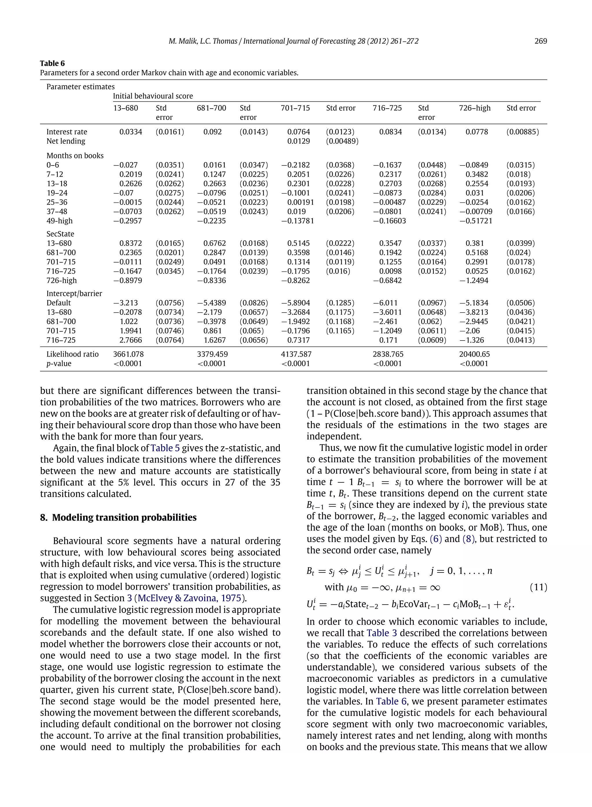

This document proposes a Markov chain model to assess the credit risk of consumer loan portfolios based on consumer behavioral scores. The key aspects of the model are: 1) It uses behavioral scores, which are calculated monthly for consumers, as an analogue to credit ratings for corporations. 2) Transition probabilities between behavioral score states are estimated using logistic regression models. 3) The model accounts for non-stationarity by including economic variables and the age of the loan as factors.