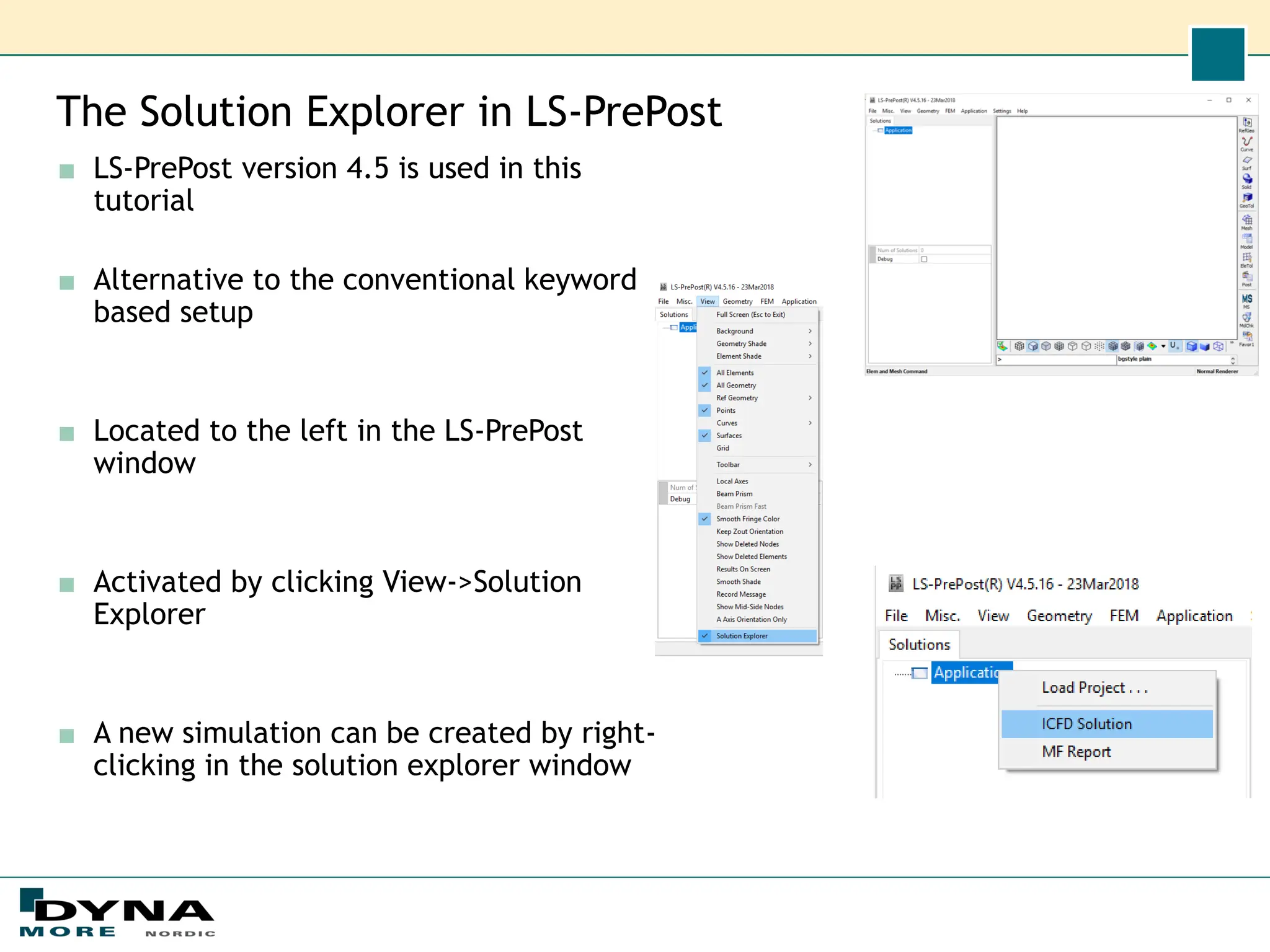
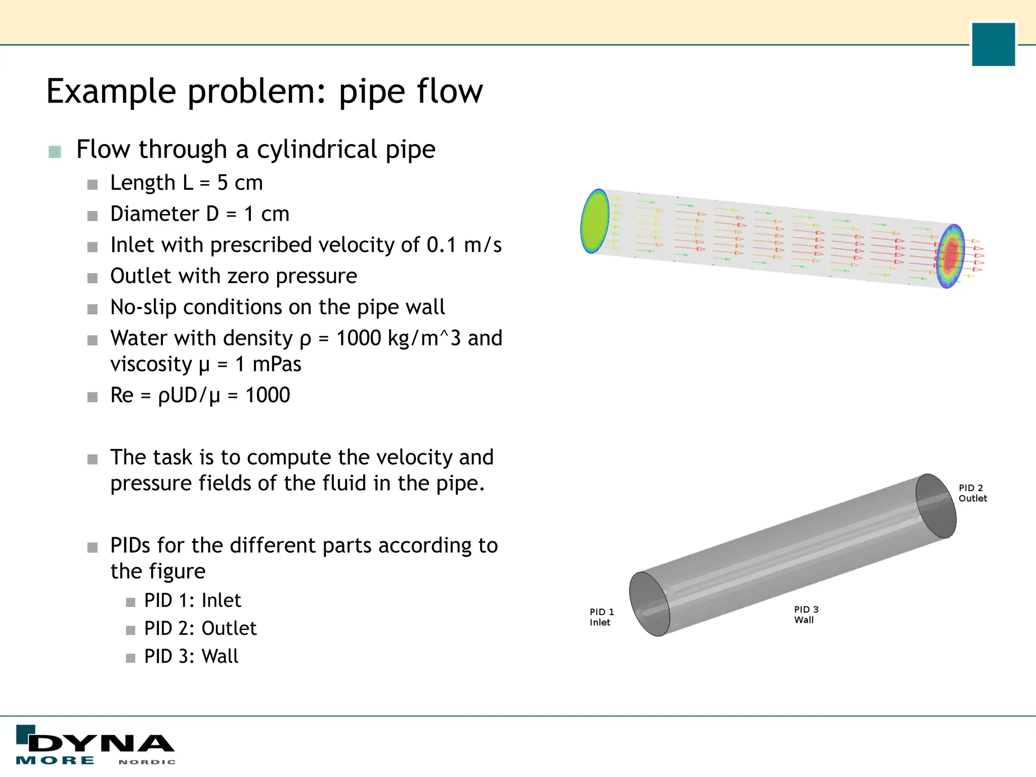
Using the new Solution Explorer in LS-PrePost
to set up an LS-DYNA ICFD simulation
Erik Svenning, PhD
DYNAmore Nordic AB
erik.svenning@dynamore.se
Purpose
■ Intro to the ICFD solver in LS-DYNA
■ The new GUI in LS-PrePost
■ Simulation setup: pipe flow
■ Post-processing
■ Summary
■ Set up a fluid flow simulation using the ICFD solver in LS-DYNA and the new
Solution Explorer GUI in LS-PrePost
■ Easier and more intuitive compared to the conventional keyword based setup
Outline
Solver introduction
■ Features of the ICFD solver in LS-DYNA
■ An implicit solver for incompressible fluids
■ Recommended to use version R9.2 or R10.1
■ Uses the Finite Element Method (FEM)
■ 2D and 3D calculations
■ Automatic volume mesh generation
■ Coupled simulations are supported
■ Fluid-Structure Interaction (FSI)
■ Conjugate heat transfer
■ Non-Newtonian fluids
■ Turbulence models
■ Porous media
■ Free surface flows (level set)
■ Steady state solver (from R10)
Model created by BETA CAE systems
The Solution Explorer in LS-PrePost
■ LS-PrePost version 4.5 is used in this
tutorial
■ Alternative to the conventional keyword
based setup
■ Located to the left in the LS-PrePost
window
■ Activated by clicking View->Solution
Explorer
■ A new simulation can be created by right-
clicking in the solution explorer window
Example problem: pipe flow
■ Flow through a cylindrical pipe
■ Length L = 5 cm
■ Diameter D = 1 cm
■ Inlet with prescribed velocity of 0.1 m/s
■ Outlet with zero pressure
■ No-slip conditions on the pipe wall
■ Water with density ρ = 1000 kg/m^3 and
viscosity µ = 1 mPas
■ Re = ρUD/µ = 1000
■ The task is to compute the velocity and
pressure fields of the fluid in the pipe.
■ PIDs for the different parts according to
the figure
■ PID 1: Inlet
■ PID 2: Outlet
■ PID 3: Wall
Creating the geometry
Create the cylinder
■ Click Solid
■ Click Cylinder
■ Radius: 0.005
■ End Pos: 0.05
■ Click Apply and
Close
Split the cylinder
surface:
■ Click Surface
■ Click Break
Surface
■ For U Parameters,
enter 0.5
■ Clear V Parameters
■ Click on the axial
edge on the
cylinder
■ Click Apply and
Close
Creating the surface mesh
■ Click Element and Mesh
■ Click Auto Mesher
■ Select Mesh Mode: Size
■ Select Mesh Type: Triangle
■ Select Elem Size: 0.001
■ Select
Connect Boundary Nodes
■ Unselect Mesh by Gpart
■ Pick the inlet face
■ Click Mesh and Accept
■ Pick the outlet face
■ Change Part ID to 2
■ Click Mesh and Accept
■ Pick the pipe wall faces
■ Change Part ID to 3
■ Click Mesh, Accept and
Done
Creating the surface mesh
■ Check that there are no
duplicate nodes.
■ Click Element Tools
■ Click Duplicate Nodes
■ Click Show Dup Nodes
■ Click Merge Dup Nodes
■ Click Accept and Done
■ Rename the parts to Inlet,
Outlet, and Wall
■ In the Feature tree, expand
FEM Parts
■ Rename LSHELL1 to Inlet by
right clicking on LSHELL1
and choosing Rename
■ Rename LSHELL2 to Outlet
■ Rename LSHELL3 to Wall
Creating the mesh
■ The next step is to save the mesh.
■ Choose File -> Save -> Save Keyword.
■ Browse to the folder where you
want to store the file.
■ As file name, enter mesh_fluid.k
■ Click Save.
■ Converting the mesh to ICFD format.
■ Here, we will convert the mesh manually. Open the
mesh file and perform the following steps:
■ Change *ELEMENT_SHELL to *MESH_SURFACE_ELEMENT.
■ Change *ELEMENT_BEAM to *MESH_SURFACE_ELEMENT.
■ Change *NODE to *MESH_SURFACE_NODE.
■ Change *PART to *ICFD_PART_TITLE.
■ Now, the mesh has been created, and we can
proceed by setting up the CFD solution using
the Solution Explorer in LS-PrePost.
Simulation setup
■ Open a new LS-PrePost
window
■ Make sure that the
Solution explorer is
visible by selecting
View->Solution
explorer
■ In the solution explorer,
right click
Application->ICFD
Solution
■ Under Model, right click
on Parts and choose
Import From Keyword
File. Pick mesh_fluid.k
■ The mesh created
previously is now visible
Fluid material
■ Right click Materials and choose Create material.
■ Click on the newly created Material1
■ Set the density to 1000
■ Set the viscosity to 0.001
■ Alternative: Right click and choose Set As Water.
Boundary conditions
■ Create boundary conditions:
■ Right click on Inlet and
choose Inflow
■ Set Value Type to Velocity
■ Set the Velocity to 0.1 m/s
■ Right click on Outlet and
choose Outflow
■ Zero pressure outlet is
default, so no further
changes are needed for the
outlet
■ Right click on Wall and
choose Wall
■ Setting mesh options:
■ By clicking on Mesh, options
for the automatic volume
mesher can be set. Here, we
will leave the meshing
options as default.
Output and time step
■ Click Output
■ Set MSGL to full output,
copied to messag file
■ Set D3plot output
frequency to 0.1
■ Click ICFD Solution
■ Set End Time to 1.0
■ Unselect Automatic time
stepping
■ Set the Time Step to 0.1
■ Right click ICFD Solution
■ Export Keyword File
■ Save the file as main.k
■ Run the simulation using
LS-Run.
■ Open the d3plot file with LS-PrePost
■ Unmark the MS_SHELL_GROUP, so that only the MS_SOLID_GROUP is active
■ Highlight MS_SOLID_5
■ Change Color by to Fluid pressure
■ In the Animate window, change to the last state
■ Now, we can see the pressure drop along the pipe
■ Right click MS_SOLID_5 and choose Section.
■ Unselect MS_SOLID_5, so that only the section plane is active.
■ Change Color by to Fluid velocity.
■ Now, we can see the velocity profile inside the pipe.
Summary
■ In this webinar, we have performed an ICFD simulation using the Solution Explorer
in LS-PrePost
■ Easier simulation setup compared to the conventional keyword based setup
■ The geometry and mesh still needs to be created as before
■ Questions and comments
■ erik.svenning@dynamore.se
Thank you!
Your LS-DYNA distributor and
more

ICFD Setup With New Solution Explorer.pdf

  • 1.
    Using the newSolution Explorer in LS-PrePost to set up an LS-DYNA ICFD simulation Erik Svenning, PhD DYNAmore Nordic AB erik.svenning@dynamore.se
  • 2.
    Purpose ■ Intro tothe ICFD solver in LS-DYNA ■ The new GUI in LS-PrePost ■ Simulation setup: pipe flow ■ Post-processing ■ Summary ■ Set up a fluid flow simulation using the ICFD solver in LS-DYNA and the new Solution Explorer GUI in LS-PrePost ■ Easier and more intuitive compared to the conventional keyword based setup Outline
  • 3.
    Solver introduction ■ Featuresof the ICFD solver in LS-DYNA ■ An implicit solver for incompressible fluids ■ Recommended to use version R9.2 or R10.1 ■ Uses the Finite Element Method (FEM) ■ 2D and 3D calculations ■ Automatic volume mesh generation ■ Coupled simulations are supported ■ Fluid-Structure Interaction (FSI) ■ Conjugate heat transfer ■ Non-Newtonian fluids ■ Turbulence models ■ Porous media ■ Free surface flows (level set) ■ Steady state solver (from R10) Model created by BETA CAE systems
  • 4.
    The Solution Explorerin LS-PrePost ■ LS-PrePost version 4.5 is used in this tutorial ■ Alternative to the conventional keyword based setup ■ Located to the left in the LS-PrePost window ■ Activated by clicking View->Solution Explorer ■ A new simulation can be created by right- clicking in the solution explorer window
  • 5.
    Example problem: pipeflow ■ Flow through a cylindrical pipe ■ Length L = 5 cm ■ Diameter D = 1 cm ■ Inlet with prescribed velocity of 0.1 m/s ■ Outlet with zero pressure ■ No-slip conditions on the pipe wall ■ Water with density ρ = 1000 kg/m^3 and viscosity µ = 1 mPas ■ Re = ρUD/µ = 1000 ■ The task is to compute the velocity and pressure fields of the fluid in the pipe. ■ PIDs for the different parts according to the figure ■ PID 1: Inlet ■ PID 2: Outlet ■ PID 3: Wall
  • 6.
    Creating the geometry Createthe cylinder ■ Click Solid ■ Click Cylinder ■ Radius: 0.005 ■ End Pos: 0.05 ■ Click Apply and Close Split the cylinder surface: ■ Click Surface ■ Click Break Surface ■ For U Parameters, enter 0.5 ■ Clear V Parameters ■ Click on the axial edge on the cylinder ■ Click Apply and Close
  • 7.
    Creating the surfacemesh ■ Click Element and Mesh ■ Click Auto Mesher ■ Select Mesh Mode: Size ■ Select Mesh Type: Triangle ■ Select Elem Size: 0.001 ■ Select Connect Boundary Nodes ■ Unselect Mesh by Gpart ■ Pick the inlet face ■ Click Mesh and Accept ■ Pick the outlet face ■ Change Part ID to 2 ■ Click Mesh and Accept ■ Pick the pipe wall faces ■ Change Part ID to 3 ■ Click Mesh, Accept and Done
  • 8.
    Creating the surfacemesh ■ Check that there are no duplicate nodes. ■ Click Element Tools ■ Click Duplicate Nodes ■ Click Show Dup Nodes ■ Click Merge Dup Nodes ■ Click Accept and Done ■ Rename the parts to Inlet, Outlet, and Wall ■ In the Feature tree, expand FEM Parts ■ Rename LSHELL1 to Inlet by right clicking on LSHELL1 and choosing Rename ■ Rename LSHELL2 to Outlet ■ Rename LSHELL3 to Wall
  • 9.
    Creating the mesh ■The next step is to save the mesh. ■ Choose File -> Save -> Save Keyword. ■ Browse to the folder where you want to store the file. ■ As file name, enter mesh_fluid.k ■ Click Save. ■ Converting the mesh to ICFD format. ■ Here, we will convert the mesh manually. Open the mesh file and perform the following steps: ■ Change *ELEMENT_SHELL to *MESH_SURFACE_ELEMENT. ■ Change *ELEMENT_BEAM to *MESH_SURFACE_ELEMENT. ■ Change *NODE to *MESH_SURFACE_NODE. ■ Change *PART to *ICFD_PART_TITLE. ■ Now, the mesh has been created, and we can proceed by setting up the CFD solution using the Solution Explorer in LS-PrePost.
  • 10.
    Simulation setup ■ Opena new LS-PrePost window ■ Make sure that the Solution explorer is visible by selecting View->Solution explorer ■ In the solution explorer, right click Application->ICFD Solution ■ Under Model, right click on Parts and choose Import From Keyword File. Pick mesh_fluid.k ■ The mesh created previously is now visible
  • 11.
    Fluid material ■ Rightclick Materials and choose Create material. ■ Click on the newly created Material1 ■ Set the density to 1000 ■ Set the viscosity to 0.001 ■ Alternative: Right click and choose Set As Water.
  • 12.
    Boundary conditions ■ Createboundary conditions: ■ Right click on Inlet and choose Inflow ■ Set Value Type to Velocity ■ Set the Velocity to 0.1 m/s ■ Right click on Outlet and choose Outflow ■ Zero pressure outlet is default, so no further changes are needed for the outlet ■ Right click on Wall and choose Wall ■ Setting mesh options: ■ By clicking on Mesh, options for the automatic volume mesher can be set. Here, we will leave the meshing options as default.
  • 13.
    Output and timestep ■ Click Output ■ Set MSGL to full output, copied to messag file ■ Set D3plot output frequency to 0.1 ■ Click ICFD Solution ■ Set End Time to 1.0 ■ Unselect Automatic time stepping ■ Set the Time Step to 0.1 ■ Right click ICFD Solution ■ Export Keyword File ■ Save the file as main.k ■ Run the simulation using LS-Run.
  • 14.
    ■ Open thed3plot file with LS-PrePost ■ Unmark the MS_SHELL_GROUP, so that only the MS_SOLID_GROUP is active ■ Highlight MS_SOLID_5 ■ Change Color by to Fluid pressure ■ In the Animate window, change to the last state ■ Now, we can see the pressure drop along the pipe
  • 15.
    ■ Right clickMS_SOLID_5 and choose Section. ■ Unselect MS_SOLID_5, so that only the section plane is active. ■ Change Color by to Fluid velocity. ■ Now, we can see the velocity profile inside the pipe.
  • 16.
    Summary ■ In thiswebinar, we have performed an ICFD simulation using the Solution Explorer in LS-PrePost ■ Easier simulation setup compared to the conventional keyword based setup ■ The geometry and mesh still needs to be created as before ■ Questions and comments ■ erik.svenning@dynamore.se
  • 17.
    Thank you! Your LS-DYNAdistributor and more