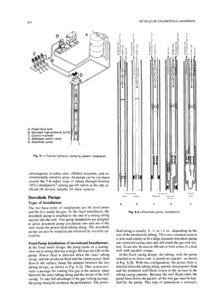
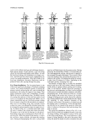
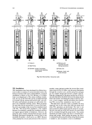
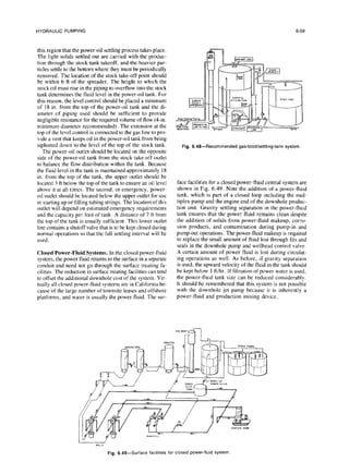
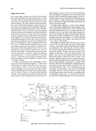
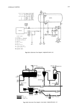
Hydraulic pumping systems use pressurized power fluid to transmit energy downhole to a downhole pump. There are two main types of installations - fixed pumps that are permanently attached, and free pumps that can be circulated in and out of the well. Free pump installations use a bottomhole assembly with a sealing shoe and seals to allow the pump to be run in and out. This allows easy removal of the pump for maintenance or replacement without pulling tubing. The power fluid can be kept separate from produced fluids in a closed-loop system, or mixed together in an open system.
![HYDRAULIC PUMPING 6-11
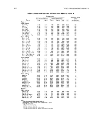
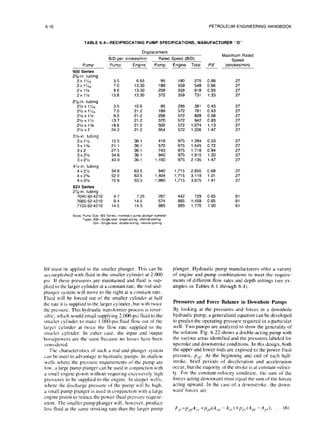
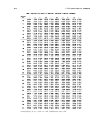
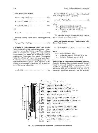
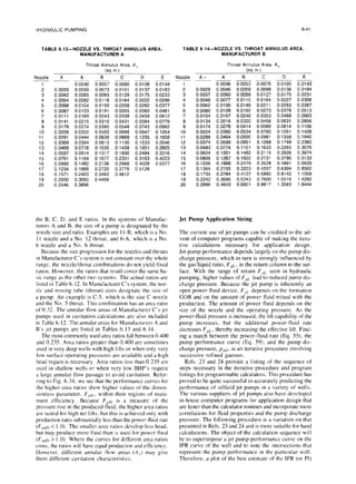
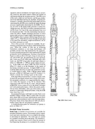
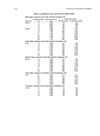
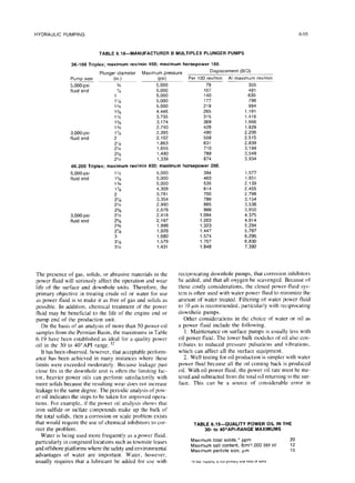
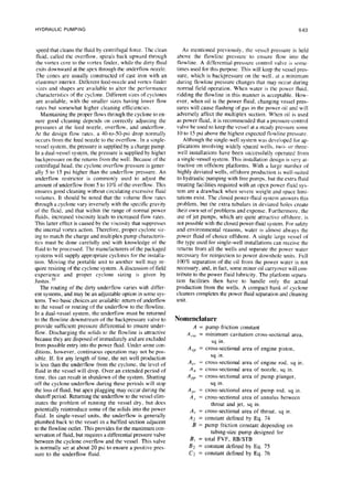
TABLE 6.1~-RECIPROCATING PUMP SPECIFICATIONS. MANUFACTURER “A”
Puma
Type F, Fe, FEB
23/8-in.
tubing
F201311
F201313
F201611
F201613
FE8201613
FE6201616
27/g-h.
tubing
F251611
F251613
F251616
FE252011
FE252013
FE252016
Type VFR
23/8-h.
tubing
VFR201611
VFR201613
VFR201616
VFR20161613
VFR20161616
27/8-h.
tubing
VFR252015
VFR252017
VFR252020
VFR25202015
VFR25202017
VFR25202020
Type V
27/-/n.
tubing
V-25-11-1
i-8
V-25-11-095
V-25-11-076
V-25-11-061
V-25-21-075
V-25-21-063
V-25-21-050
V-25-21-041
Type 220
23/-h. tubing
330-201610
330-201612
530-201615
27/-h. tubing
348-252012
348-252015
548-252017
548-252019
536-252020
Note Pump Size
F. FE, FEB. VFR Types
F
Disolacement
B/D oer strokeslmin
Puma
3.0 4.2
4.2 4.2
3.0 6.4
4.2 6.4
6.2 9.4
9.4 9.4
3.3 7.0
4.6 7.0
7.0 7.0
5.0 16.5
7.0 16.5
10.6 16.5
2.12 4.24
2.96 4.24
4.49 4.24
2.96 6.86
4.49 6.86
5.25 8.89
7.15 8.89
9.33 8.89
5.25 15.16
7.15 15.16
9.33 15.16
6.31 5.33
6.31 6.66
3.93 5.33
3.93 6.66
6.31 8.38
6.31 10.00
3.93 8.38
3.93 10.00
4.22 8.94
5.46 8.94
7.86 8.94
8.73 22.35
12.57 22.35
17.11 22.35
20.17 22.35
25.18 25.18
V Types
v
220 Sertes
3 Number of seals
20 Nommal tubing (2 I” ) 25 Nommal tubmg (2% I” ) 48 Stroke length p,
13 Engme (1 3 I” ) 11 Single engme (double = 21) 25 Nomlnal tubing (2% in.]
XX Second engine (VFR only) 118PIE 20 Engine (2 000 IO.)
11 Pump (1 1 in ) 12 Pump (1 200 m.)
Types F. FE. FEB are slngle-seal, internal-portmg; 220, VFR, and V are multiple-seal, external-pomng.
Engine
Rated Speed (B/D)
Enaine Total PIE
Puma
204
285
204
285
340
517
214
299
455
255
357
540
318
444
673
444
673
630
8.58
1,119
630
858
1,119
1,229
1,299
550
550
1,173
1,072
550
550
422
546
786
629
905
1,232
1,452
2,014
286 490 0.71
286 571 1.00
435 639 0.47
435 720 0.66
517 857 0.66
517 1,034 1.00
455 669 0.47
455 754 0.66
455 910 1.00
842 1,097 0.30
842 1,199 0.42
842 1.382 0.64
636 954 0.62
636 1,080 0.87
636 1,309 1.32
1,029 1,473 0.54
1,029 1,702 0.81
1,067 1,697 0.74
1,067 1,925 1.00
1,067 2,186 1.32
1,819 2,449 0.41
1,819 2,677 0.56
1,819 2,938 0.73
1,098 2,397 1.18
1,372 2,671 0.96
746 1,296 0.76
932 1,482 0.61
1,559 2,732 0.75
I;700 23772 0.63
1,173 1,723 0.50
1,400 1,950 0.41
894 1,316 0.49
894 1,440 0.63
894 1.680 0.89
1,609 2,238 0.40
1.609 2.514 0.57
11609 2,841 0.78
1,609 3,061 0.93
2,014 4,028 1.00
Maximum Rated
Speed
(strokes/min)
68
68
68
68
ii;
65
65
65
51
51
51
150
150
150
150
150
120
120
120
120
120
120
206
206
140
140
186
170
140
140
100
100
100
72
72
72
72
80](https://image.slidesharecdn.com/hydraulicpumping-220105163948/85/Hydraulic-pumping-10-320.jpg)
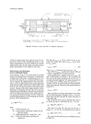
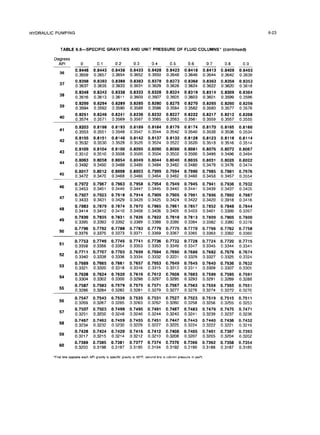
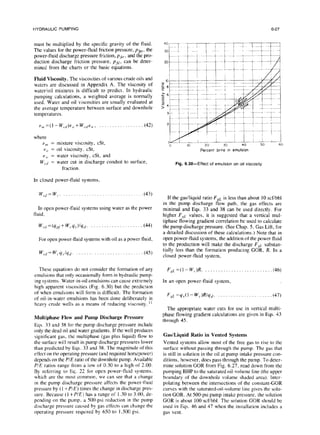
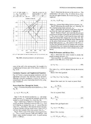
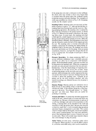
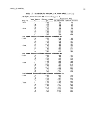
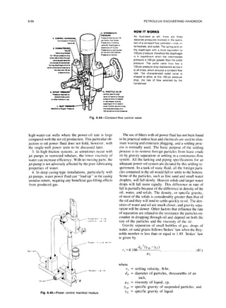
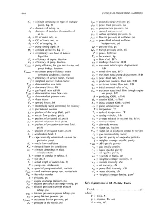
![HYDRAULIC PUMPING 6-17
Powerlift
I Powerlift
II
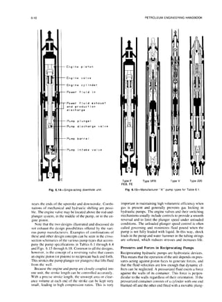
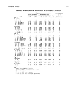
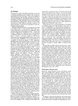
Fig. 6.17-Manufacturer “C” pump types forTable 6.3
where
F,, = downward force, Ibf,
P,]~ = power-fluid pressure, psi,
A<‘r-
- cross-sectional area of engine rod, sq in.,
AL’,’= cross-sectional area of engine piston.
sq in.,
PP> = pump suction pressure, psi,
A PP = cross-sectional area of pump plunger,
sq in., and
AP’ = cross-sectional area of pump rod, sq in.
The upward forces are
where
F,, = upward force, Ibf,
pcl/ = engine discharge pressure, psi, and
p,,‘l = pump discharge pressure. psi.
900 Series
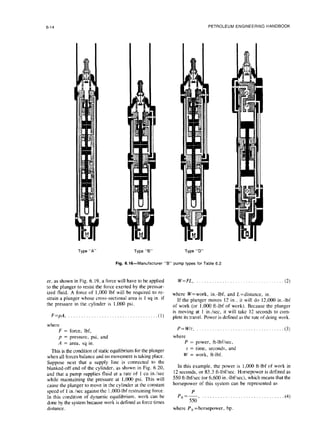
Fig. &la-Manufacturer “D” pump types forTable 6.4
924 Series
Equating the upward and downward forces and solving
for the power-fluid pressure at the pump gives
P,,~=P<,<I
+P~JA,,~ -A,rY(A,, -A,,.)
-p,u(A, -A,,Y(A, -A<,,). . .(8)
If PPCi
=pF/, as is the case in open power-fluid systems,
then
~,>t.=~,d’ +(A, -A,,V(*,,,, -*,,)I
-P,JA, -A,,V(A, -A,,). .(9)
Eq. 8 can also be written as
P/~=P~,~/+(P~~-P,,~)[(A,,~ -A,,V(A, -Aw)l.
. . . . . . . . . . . . . . . . . . . . . ..__.. (10)](https://image.slidesharecdn.com/hydraulicpumping-220105163948/85/Hydraulic-pumping-16-320.jpg)
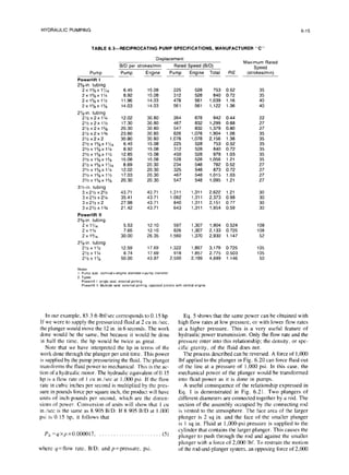
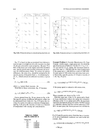
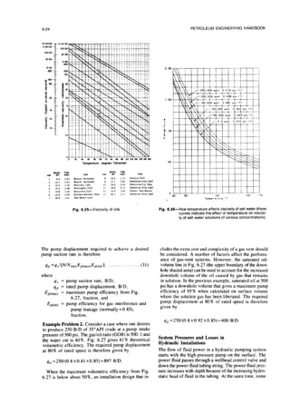
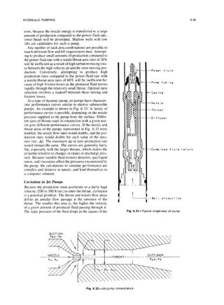
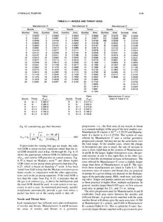
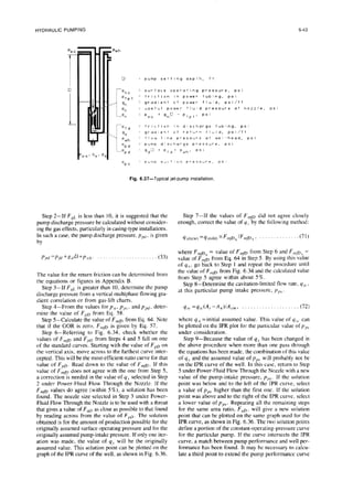
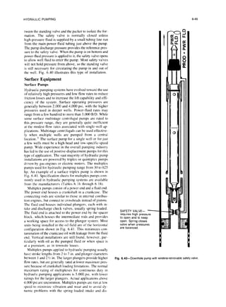
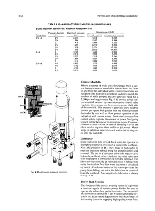
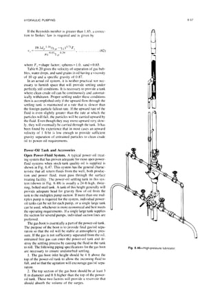
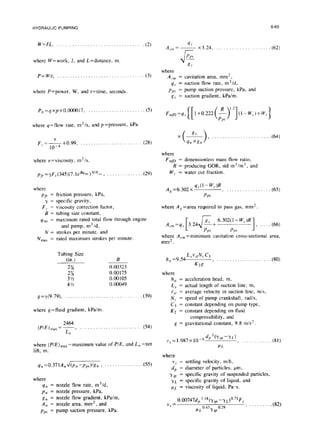
![6-18 PETROLEUM ENGINEERING HANDBOOK
-Force : lb
/
L Area of face of plunger : I in2
f!Fluid pressure = 1000 psi i Fluid pressure : 1000 psi
Fig. 6.19-Pressure and force ina static
plunger and cylinder
assembly.
Fig. 6.20-Pressure, force,and flow ina dynamic plunger and
cylinderassembly.
The same analysis for the upstroke would give the same
answer because this double-acting pump is completely
symmetrical.
Fig. 6.23 shows a balanced downhole unit with a single-
acting pump end. First, for the downstroke. the down-
ward forces are
F,I =P,>~(A,,J +p,,, (A,,,, -A,,), __, .(]I)
and the upward forces arc
F,, =P,,/(A,,, -A,,-) +/~,,/(A,,. -AP’.)+p,dA,,,‘)
. . . . . . . . . . . . . . . . . . . . . . . . . . (12)
In this pump. the areas of the engine and pump rods are
half that of their respective pistons and plungers:
A,,.=A,,/2 . . ..(13)
and
A,],.=A,,,J2. (14)
Equating the upward and downward forces, substituting
Eqs. 13 and 14, and solving for the power-fluid pressure.
P,,/ 8 g*ves
~,,~=~,dl +A,~,,IA,)-p,,,(A,,IA,). (15)
Evaluating the force balance for the upstroke gives
F,/ =P c,r/
(Ac,>
)i-p,> (A,,,I-A,,.) _. (16)
and
..,....,,....,,,,.,.,.,.,,, (17)
Eqs. 13. 14, 16, and 17 give
~pr = 21’,></
-p,d 1-A ,,,I/A e,,)-I’,” (A,,, /Ac/l). (18)
Note that if prcf =ppn, which is the case in an open
power-fluid installation, Eqs. 1.5and 18 become the same:
p,,/=~,x/(l +A,/*,,,)-p,,,,(A,,,,IA,). .(19)
Eq. 19 for the single-acting pump shown in Fig. 6.23 can
be made identical to Eq. 9 for the double-acting pump
shown in Fig. 6.22 by observing that, because of Eqs.
13 and 14,
A,/A, =(A,,,, -A,,)/(A, -A,,). . (20)
Because it appears frequently in pressure calculations
with hydraulic pumps, the term (A,,p -A,,,.)/(A,,,l -A,,)
is frequently simplified to P/E. This is sometimes called
the “P over E ratio” of the pump and is the ratio of the
net area of the pump plunger to the net area of the engine
piston. With this nomenclature. Eq. 8 for a closed power-
fluid installation becomes
P/f=Ped +p~d(PIE)-p,,,~(PIE), (21)
where PIE=(A, -*,,.)/(A, -A,,.).
Eq. 9 for an open power-fluid installation becomes
~,,~=p,,(,[ 1+ (PIE)] -pps(PIE). . . (22)
This approach has found widespread acceptance among
the manufacturers of downhole pumps, and the ratio P/E
is included in all their pump specifications (see examples
in Tables 6.1 through 6.4).
P/E values greater than 1.Oindicate that a pump plunger
is larger than the engine piston. This would be appropri-
ate for shallow, low-lift wells. P/E values less than 1.0
are typical of pumps used in deeper. higher-lift wells. In
some pumps, the P/E value is also the ratio of pump dis-
placement to engine displacement, but corrections for fluid](https://image.slidesharecdn.com/hydraulicpumping-220105163948/85/Hydraulic-pumping-17-320.jpg)
![6-28 PETROLEUM ENGINEERING HANDBOOK
Pressure Relationships Used
To Estimate Producing BHP
The pressure relationships of Eqs. 2 1and 22 can be rear-
ranged to give the pump intake pressure p,,, in terms of
the other system pressures and the PIE ratio of the pump.
For the closed power-fluid system,*
For the open power-fluid system,
j7,' =p,,‘/-(p,l,-p,,,,)/(P/E). (49)
If the appropriate relationships from Eqs. 32 through
38 are used. the equation for the closed power-tluid system
becomes**
-(plr,+X,,l.D+P,,h~,)]I(PIE), (50)
where g, =x(1 in a closed power-fluid system.
For the open power-tluid system, the relationship is
-(pf;,+g,,D+P,,,,)]/(P/E). ., ..(51)
These equations can be used directly. but several prob-
lems arise. Several friction terms must be evaluated, each
with a degree of uncertainty. The term p,. for the losses
in the pump is the least accurate number because pump
wear and loading can affect it. To avoid the uncertainty
in friction values. a technique called the “last-stroke
method” is often used. With this method. the power-tluid
supply to the well is shut off. As the pressure in the sys-
tem bleeds down. the pump will continue to stroke at slow-
er rates until it takes its last stroke before stalling out.
The strokes can be observed as small kicks on the power-
fluid pressure gauge at the wellhead. The power-fluid
pressure at the time of the last stroke is that required to
balance all the fluid pressures with zero flow and zero
pump speed. At zero speed. all the friction terms are zero,
cxccpt p/,., which has a minimum value of SOpsi. which
simplifies Eqs. 50 and 5 I. With the friction terms re-
moved, the last stroke relationship for the closed power-
fluid system becomes
(g,,tD+P,,,lrc,)]/(P/E). (52)
For the open power-fluid system the relationship is
-(,~I,D+l,,,.,,)II(PIE). (53)
‘Eq 48 IS dewed from Eq 21 and Eq 49 IS dewed from Eq 22
“Eq 50 IS dewed lrom Eq 21 and Eq 51 IS dewed from Eq 22
These relationships have proved to be very effective in
determining BHP’s. ” However, they are limited to wells
that produce little or no gas for the reasons discussed in
the section on Multiphase Flow and Pump Discharge Pres-
sure. Eqs. 50 and 51 can be used in gassy wells if the
hydrostatic-pressure and flowline-pressure terms arc re-
placed by a pump discharge pressure from a vertical mul-
tiphase flowing gradient correlation. The equations for
the last-stroke method, however, present a further prob-
lem because they require the gradient at a no-flow condi-
tion. The multiphase-flow correlations show a significant
variation of pressure with velocity. Wilson, in Brown,’
suggests subtracting the friction terms from the flowing
gradient for evaluating Eqs. 52 and 53 or attempting to
determine pf,. more accurately for use in the evaluation
of Eqs. 50 and 5 I, The method suggested here is to use
a multiphase-flow correlation for determining ~~~~1
at the
normal operating point of the pump. With the same cor-
relation for the same proportions of liquid and gas, de-
termine what the pPll pressure would be at a low tlow
rate, corresponding to the conditions when the pump is
slowing down to its last stroke. By plotting the two values
of p,,(/ obtained, we can extrapolate to what pprl would
be at zero flow. This value can be used to replace the
hydrostatic-head and flowline-pressure terms.
Selecting an Appropriate PIE Ratio. As previously dis-
cussed, large values of P/E are used in shallow wells and
small values in deeper wells. The larger the value of P/E,
the higher the surface operating pressure to lift fluid
against a given head will be. The multiplex pumps offered
by the manufacturers are rated up to 5,000 psi, but few
hydraulic installations use more than 4,000 psi except in
very deep wells. About 80 to 90% of the installations use
operating pressures between 2,200 and 3,700 psi. With
the simplifying assumptions of an all-water system, no
friction, 500-psi pump friction, 4,000-psi operating pres-
sure. and a pumped-off well, Eqs. 22, 33, and 36 lead to
(P/E),,,, =3,500/0.433/l,, =8.000/L,,, . . . . . . ..(54)
where L,, =net lift, ft.
Eq. 54 is useful in initial selection of an appropriate
PIE ratio in installation design. The actual final determi-
nation of the surface operating pressure will depend on
calculation of the actual gradients and losses in the sys-
tem and on the particular pump’s P/E ratio.
Equipment Selection and Performance Calculations
Equipment selection involves matching the characteris-
tics of hydraulic pumping systems to the parameters of
a particular well or group of wells. A worksheet and sum-
mary of equations are given in Table 6.7.
Once a downhole unit has been selected and its power-
fluid pressure and rate determined. an appropriate power
supply pump must be matched to it. The section on sur-
face equipment and pumps provides a detailed descrip-
tion of the types of pumps used for powering hydraulic
pumping systems. Specifications for some of the pumps
typically used can be found in Tables 6. I through 6.4
(Figs. 6.15 through 6.18).
A troubleshooting guide is provided in Tables 6.8
through 6. IO.](https://image.slidesharecdn.com/hydraulicpumping-220105163948/85/Hydraulic-pumping-27-320.jpg)
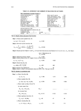
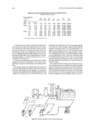
![HYDRAULIC PUMPING 6-29
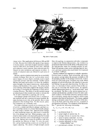
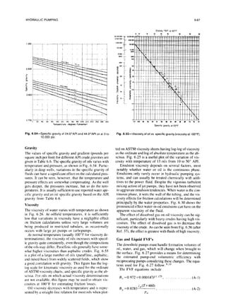
TABLE 6.7-WORKSHEET AND SUMMARY OF EQUATIONS FOR RECIPROCATING PUMPS
Well Identification
Example Problem 3
Vertical
setting
depth, ft 9,000
Tubing length,ft 9000
Tubing ID,in. 2.441
Tubrng OD, In. 2.875
Return ID, in. 4.892
Wellhead pressure,psi 100
Gas specific
gravity 0.75
011gravity,
“API 40
Power fluid
specific
gravity 0.82
Produced 011specific
gravtty 0.82
Water specific
gravity
Power fluid
gradient,
psiift
Produced oilgradient,psilft
Water gradient,psilft
Oilviscosity,
cSt
Water viscosity,
cSt
GOR, scflbbl
Water cut,%
Surface temperature, OF
Bottomhole temperature, OF
1.03
0.357
0.357
0.446
2
0.485
100
70
100
200
Expected net lift,
ft 7,800 Vented? Yes- No2
Desired production,B/D 250
Pump intakepressure at above rate,psi 500
Installation:
Casing i/ Parallel
_
OPF r, CPF
Step 1 -(P/O max
=8,000/L, = 1.03 (Eq. 54)
Step a--Maximum pump efficiency
Eprmax,
(Fig.6.27)
97
% (Vented)
% (Unvented)
Step 3-Minimum recommended pump displacement (Eq. 31):
qp =9,/; ~Epmax, xEp~,nt,
= 250/(0.8x0.97 x 0.85)= 379 B/D
max
Step 4-Select pump from Tables 6.1 through 6.4 with P/E lessthan or equal to value from Step 1 and a maximum rated
pump displacement equal to or greaterthan the value from Step 3
Pump designation:
Manufacturer B Type A 2% x 11/4-11/4
in.
PIE 1.oo
Rated displacement, B/D 492
Pump, BIDlstrokeslmin 4.92
Engine, BIDlstrokeslmin 5.02
Maximum rated speed, strokes/min 100
Step S-Pump speed:
N= qsW,~,,xl x Epc,ntr)l2WO.97xO.W
q,lN,,x =
= 61.6 strokes/min
4921100
Step B-Calculate power-fluid
rate(assume 90% engine efficiency,
E,)
qpf= N(q,/N,,,)/E, = 61.6(502/100)/0.90
= 344 B/D
Step 7-Return fluid
rateand properties-OPF system
a. Totalfluid
rate: power fluid
rate,
qp, = 344 BID
+ productronrate,9r = 250 BID
= totalrate,
qd = 594 BID
b.Water cut:
Water power fluid
(Eq. 44)
WC, = (9Pf+ W,q,)J9, =
Oil power fluid
(Eq. 45)
wcd=wcq,/q,=07x250/594=o.29
c. Vscosity (Eq.42)
v,,,
=(I - Wcd)vo + Wcdvw =(I -0.29)2+0.29x0.485= 1.56 cSt
d. Suction gradient(Eq. 40)
gs=g~(l-W,)+g,W,=0.357(1-0.7)+0.446x0.7=0.419psl/fi
e. Return gradient(Eq 41)
gd = [(9,(
xg,,) +(9s xg,)]/q, =[(344x 0.357)+(250 x0.419)1/594=0.383 psrlft
f. Gas/liquidratro
(Eq. 47)
F,, =q,(l - W,)R/q,=250(1 -0.7)100/594=12.6 scilbbl
Note: For vented installations,
use solutionGOR (Frg.6.27)](https://image.slidesharecdn.com/hydraulicpumping-220105163948/85/Hydraulic-pumping-28-320.jpg)
![6-30 PETROLEUM ENGINEERING HANDBOOK
TABLE 6.7-WORKSHEET AND SUMMARY OF EQUATIONS FOR RECIPROCATING PUMPS (continued)
Step B-Return fluid
ratesand properties-closed power-fluid
systems. Because the power fluid
and produced fluid
are kept
separate,the power returnconduit carriesthe flow ratefrom Step 6, with power-fluid
gradientand viscosity.
The production
returnconduit carriesthe desired production ratewith productiongradient,
water cut,viscosity,
and GOR.
a. Power-fluid
returnrate BID
b. Production returnrate BID
Step g--Return friction:
Ifa gas lift
chart or vertical
multiphase flowinggradientcorrelation
(see Chap. 5) isused forreturn
flow calculations,
itwill
already includefriction
values and the flowline
backpressure. Use of gas lift
chartsor correlations
is
suggested if
the gas/liquid
ratio
from Step 7 isgreaterthan IO.The value from such a correlation
can be used directly
in Step
llc withoutcalculating
friction
values. Ifa gas-lift
chart or vertical
flow correlation
isnot used, then with the values from Steps
7 and 8, as appropriate,
determine the returnconduit friction(s)
from the chartsor equations inAppendix 6.
1.Open power-fluid
friction
pfd = psi.
2. Closed power-fluid
friction
a. power returnpter
=- psi.
b. production returnptd=- psi.
Step lo-Power-fluid friction:
With the power-fluid
ratefrom Step 6, use the appropriatechartsor equations in Appendix B to
determine the power-fluid
friction
loss.
Power fluid
friction
prpt= 4.4 psi.
Step 11-Return pressures:
a.Open power-fluid
system (Eq. 33)
Ppd=Pfd+i?dD+P,= psi.
b.Closed power-fluid
system (Eqs. 37 and 38)
1.P ed=Plet+!?~D+Pwhe=--- psi
2.P,d=P,+!7,D+P,= psi
c. Ifa vertical
multiphase flowinggradientcorrelation
ISused insteadof Eqs. 33, 37, or 38, then ppd =3,500 psi,
Step 12-Required engine pressure ppf:
a. Open power-fluid
system (Eq. 22)
p,,=ppd[l+(P/E)]-pps(P/E)=3,500[1+1]-500(1)=6,500psi.
b.Closed power-fluid
system (Eq. 21)
Ppf ‘Ped +Ppd(PIE)-Pp,(PIE)= psi
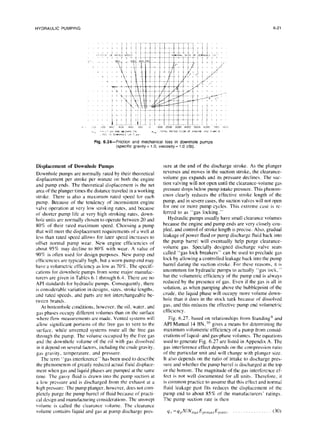
Step 13-Calculate pump friction
a. Rated pump displacement,qp =492 B/D
b. Rated engine displacement,qe = 502 B/D
c.Totaldisplacement,qtm = 994 B/D
d. “8” value (Table 6.5)= 0.000278
e. N/N,,, = 61.61100=0.616
f.f,=~/100+0.99=2/100+0.99=1.01 (Eq. 28)
g. Pump friction
(Eq. 29 or Fig.6.24)
pb =yF,(50)(7.1ee9” jNINmax
plr=0.82(1.01)(50)[7.1eoooo278~994~]06’6
= 164 psi.
Step 14-Required surface operatingpressure p, (Eq. 36):
pso =pp, +ptpf-gprD+pr, =6,500+4.4-0.357(9,000)+ 164=3:455 psi
Step 15-Required surface horsepower, assuming 90% surface efficiency
(Eq. 5):
P, =qp,xp,, x0.000017/E, =344x3,455x0.000017/0.9=22.4 hp.
Step 16-Summary:
Pump designation-Manufacturer B Type A 21/z
x 1X-1% in.
Pump speed, strokeslmin 61.6
Production rate,B/D 250
Power fluid
rate,B/D 344
Power fluid
pressure,psi 3,455
Surface horsepower 22.4
Step 17-Triplex options (from manufacturer specification
sheet,Tables 6.16 through 6.18):
Type
J-30 D-323-H
Plunger size,in. 1% 1‘/a
Revolutionslmin 450 300
Flow rateat revolutionslmin
(B/D) 400 399
Maximum pressure rating,
psi 3,590 4.000
Horseoower 26 26](https://image.slidesharecdn.com/hydraulicpumping-220105163948/85/Hydraulic-pumping-29-320.jpg)
![HYDRAULIC PUMPING 6-45
TABLE 6.15-WORKSHEET AND SUMMARY OF EQUATIONS FOR JET PUMPS (continued)
Step P-Discharge pressure (Eq. 31) ifF,, i 10
pld from Appendix B. Pfd =-
P/,d =/‘fd +SdD+Pwh Ppd =
Step 3-Use vertical
multiphase flow correlation
ifFg, > IO to determine ppd
ppd = 1,780
Step 4-Calculate pressure ratio
(Eq. 58)
Fpo =(ppd -P~~Y(P~ -P& F,, = 0.318
Step 5-Calculate mass flow ratio
(Eq. 64)
F ~~~[1+~~8(~~“]~~-~,1+~~~~~
mm = F m,D,=0.791
9,X9”
1,756
0.305
1.04
1,746
0.300
1.09
Step g--Use value of F,, in Fig.6.34 to findF,,D from farthest
curve to right
at thatvalue of F,,. Note value of F,,.
F,, = 0.25 0.25 0.25
F mKJg =1.04 1.06 1.10
Step 7-Compare Fmfog from Step 5 with FmfDs from Step 6. IfwithinV/o, go to Step 8. Ifnot,correctqs by Eq. 71.
qspew)= q,~o,,,FmrD,
‘Fnm5
then returnto Step 6.1.a
9 sinewi
= 657 670 676
Part C-Hardware and finalcalculations
Step l-Pick throatsizeclosestto
A, = F =0.0412 sq in. Actual throatarea = 0.0441
al? size= 9
Step 2-Cavitation limited
flow (Eq. 72)
A,-An
9,,=4s,xy-
cm
qsc = 1,037
Step 3-Hydraulic horsepower (Eq. 5)
P, =q* xp,, x0.000017
Step 4-Triplex power at 90% efficiency
P, =35
=39
A, =0.0103 p so= 2,500 qs= 676
A, = 0.0441 qn= 820 P ps= 1,000
I= = 0.235
aD P,= 39
Triplexoptions(from manufacturer specification
sheet,Tables 6.16 through 6.18)
Type
D-323-H J-60
Plunger size,in. 1% 1%
revlmin 400 400
Flow rateat revlmin,B/D 945 945
Maximum rating,
pressure psi 2,690 2,690
Horsepower 44.6 44.6
K-l00
1a/4
221
945
2,740
44.6](https://image.slidesharecdn.com/hydraulicpumping-220105163948/85/Hydraulic-pumping-44-320.jpg)

![HYDRAULIC PUMPING
6-69
The compressibility of gas is a function of three
variables-gas specific gravity. temperature. and pressure.
for turbulent tlow, where
Q =f(yK, T, p). . .(A-@
A gas compressibility equation programmed for the
computer relates these variables as follows:
i,=A+Bp,+(l-A)e-‘-H(p,/10)~, _. (A-9)
where
AP, =
p=
pip =
L=
9=
d=
yP=
f=
=
=
friction pressure drop, psi,
weighted average viscosity. up.
weighted average kinematic viscosity, cSt,
length of tubing. ft,
quantity of oil flowing, B/D.
ID of tubing, in.,
weighted average specific gravity,
weighted average friction factor
WwG)
0.0361 (~I~)".z'/(dv)O~l'.
A=-0.101-0.36T,+1.3868(T,-0.919)”5. (A-10)
Transition from laminar to turbulent flow occurs when
the Reynolds number (NR~) is greater than 1,200.
B=0.021+0.04275/(7--0.65).
r,=(T+460)/(175+307y,),
p,=p~~/(701-47y,).
C=p,(D+Ep,+Fpr4). .
D=0.6222-0.224T,.. . . . .
E=O.O657/(T,-0.86)-0.037,
~=0.32~l-19.53’r~-1)1, _.
and
...... (A-l 1)
...... (A- 12)
...... (A-13)
...... (A-14)
...... (A-15)
...... (A-16)
...... (A-17)
H=0.]22e]-ll.“‘TI-~“I , .,,,........,.... (A-18)
where
Pi- = reduced pressure, and
T, = reduced temperature.
Appendix B-Friction Relationships
Because hydraulic pumping systems require greater cir-
culating volumes of fluid than other artificial lift systems,
the proper determination of friction losses is important.
This subject is thoroughly covered by F.B. Brown and
C.J. Coberly38 and includes the effect of viscosity gra-
dients, laminar to turbulent transitions, proper equivalent
diameters for annulus passages, and tubing eccentricity
in casing/tubing annular flow passages. Their results are
summarized in the following equations.
Circular Sections-Tubing
~=0.01191~. . . . . . . . . . . . . . . . . . . . . . . . ..(B-1)
where
v = velocity, ftisec,
q = quantity of oil flowing, B/D, and
d = diameter of tubing, in.
Ap/=7.95x10-6$ . . . . . . .(B-2)
for laminar flow and
Ap~=N46&~$ . . ..t...... (B-3)
G-4)
Annular Sections-Flow Between Tubing and Casing
Laminar flow:
~=0.01191
9
d,2-d22
and
APT=
(d, -d2)2(dl’ -dzz)(1+l.5e’)’ “’
(B-6)
where
Ap, = friction pressure drop, psi,
p = weighted average viscosity, cp.
L = length of annulus, ft,
q = flow, B/D.
d, = ID of outer tube, in.,
dz = OD of inner tube, in.,
e = eccentricity of tubes=2d3/(d I -d?), and
d3 = distance inner tube is off center, in.
Turbulent Flow:
Ap’.f
=
(d, -d*)(d, 2-dz2)2
where
Appt.=
GE
L=
yQ=
friction pressure drop, psi,
flow, B/D,
length of annulus, ft,
weighted average specific gravity
(water= 1.O),
dl = ID of outer tube, in.,
dz = OD of inner tube, in.,
d3 = OD of coupling (inner tube), in..
e= eccentricity=(d, -d3)/(d1 -d2),
J‘= @(dvplp) =0.0361(Flp)“~2’ /(dv)“,2’, and
dP = weighted average kinematic viscosity, cSt.
. . . . . . . . . . . . . . . . . . . . . . . . . . (B-7)](https://image.slidesharecdn.com/hydraulicpumping-220105163948/85/Hydraulic-pumping-68-320.jpg)