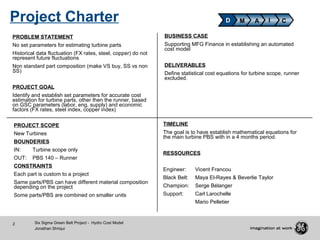
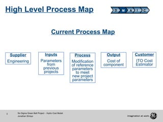
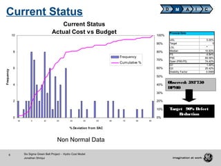
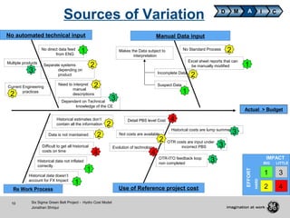
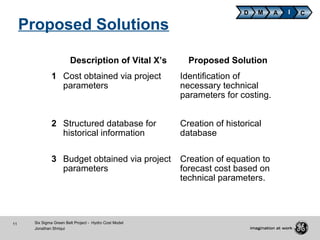
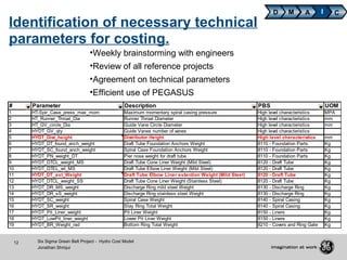
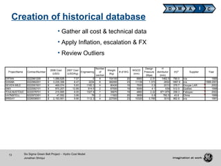
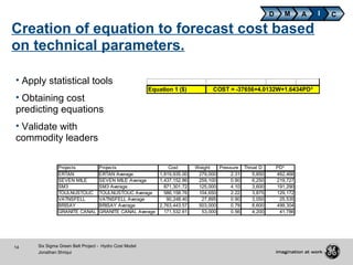
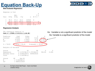
Hydro Cost Model – Turbine Equations
Six Sigma Green Belt Project
Project ID – A112502.2
Jonathan Shriqui
February 2007
2 Six Sigma Green Belt Project - Hydro Cost Model
Jonathan Shriqui
D M A CI
PROBLEM STATEMENT
No set parameters for estimating turbine parts
Historical data fluctuation (FX rates, steel, copper) do not
represent future fluctuations
Non standard part composition (make VS buy, SS vs non
SS)
PROJECT GOAL
Identify and establish set parameters for accurate cost
estimation for turbine parts, other then the runner, based
on GSC parameters (labor, eng, supply) and economic
factors (FX rates, steel index, copper index)
BUSINESS CASE
Supporting MFG Finance in establishing an automated
cost model
DELIVERABLES
Define statistical cost equations for turbine scope, runner
excluded.
PROJECT SCOPE
New Turbines
BOUNDERIES
IN: Turbine scope only
OUT: PBS 140 – Runner
CONSTRAINTS
Each part is custom to a project
Same parts/PBS can have different material composition
depending on the project
Some parts/PBS are combined on smaller units
TIMELINE
The goal is to have establish mathematical equations for
the main turbine PBS with in a 4 months period.
RESSOURCES
Engineer: Vicent Francou
Black Belt: Maya El-Rayes & Beverlie Taylor
Champion: Serge Bélanger
Support: Carl Larochelle
Mario Pelletier
Project Charter
3 Six Sigma Green Belt Project - Hydro Cost Model
Jonathan Shriqui
D M A CI
Current Process Map
Customer
ITO Cost
Estimator
Output
Cost of
component
Process
Modification
of reference
parameters
to meet
new project
parameters
Inputs
Parameters
from
previous
projects
Supplier
Engineering
High Level Process Map
4 Six Sigma Green Belt Project - Hydro Cost Model
Jonathan Shriqui
D M A CI
• Cost estimations are based on reference projects, where the
data and technology used at that time may now be outdated
• Highly manual process, no standardization
• Requires high product knowledge
• No standard template for estimators
• Limited relevant historical data
“As Is” Process Weakness
5 Six Sigma Green Belt Project - Hydro Cost Model
Jonathan Shriqui
D M A I CDefine Performance Standards
What is a defect:
Budget variation from Actual cost greater then 5%
What is being measured?
Actual cost vs budget
Performance Standard and Specification Limit
•Type of Data: Discrete
•Opportunity: All turbine components (runner excluded)
•Defect Definition:
Acceptable%5
costBudget
costBudget-costActual
DEFECT%5
costBudget
costBudget-costActual
=





≤
=





>
6 Six Sigma Green Belt Project - Hydro Cost Model
Jonathan Shriqui
Current Status
Actual Cost vs Budget
0
2
4
6
8
10
-10 0 10 20 30 40 50 60 70 80 90
% Deviation from EAC
Frequency
0%
10%
20%
30%
40%
50%
60%
70%
80%
90%
100%
Frequency
Cumulative %
D M A CI
Observed: 593’750
DPMO
Target 90% Defect
Reduction
Process Data
USL 5.00%
Target 0
LSL *
Median 10.83%
P5 -4.84%
P95 69.58%
Span (P95-P5) 74.42%
Q1 1.49%
Q3 25.42%
Stability Factor 0.0585
Non Normal Data
Current Status
7 Six Sigma Green Belt Project - Hydro Cost Model
Jonathan Shriqui
DELIVERABLE
Mathematical equation (transfer function) based on measurable parameter(s) delivering
an accurate estimation with a 95% confidence level.
Y=F(X) where R2
< 95%
D M A CIDeliverable Definition
8 Six Sigma Green Belt Project - Hydro Cost Model
Jonathan Shriqui
Performance Objectives D M A CI
Y=F(X) where R2
> 95%
Target:
To reduce all cost estimation defects, where the variation
between actuals & budget would +- 5%.
Business CTQ: Accuracy
Performance Std: Forecast a cost within 5% of its actual cost
9 Six Sigma Green Belt Project - Hydro Cost Model
Jonathan Shriqui
Baseline Z D M A CI
Zone of Average
Technology
Zone of
Typical
Control
0.0
0.5
1.0
1.5
2.0
2.5
3.0
0 1 2 3 4 5 6
Z.Shift
Z.Bench (Short-Term)
World-Class
Performance
Report 8B: Product Benchmarks
1
10
100
1000
10000
100000
1000000
0 1 2 3 4 5 6
Z.Bench (Short-Term)
PPM
Report 8A: Product Benchmarks
Z(bench) = 1.2 (593’750 DPMO)
* Product Report – Discreet Data
10 Six Sigma Green Belt Project - Hydro Cost Model
Jonathan Shriqui
Sources of Variation
Actual > Budget
No automated technical input Manual Data input
Re Work Process Use of Reference project cost
EASY
OTR-ITO feedback loop
non completed
Detail PBS level Cost
Data is not maintained
Incomplete Data
Suspect Data
Makes the Data subject to
interpretation
No direct data feed
from ENG
Multiple products
Separate systems
depending on
product
Current Engineering
practices
Need to interpret
manual
descriptions
Difficult to get all historical
costs on time
Historical data not inflated
correctly
Excel sheet reports that can
be manually modified
No Standard Process
Dependent on Technical
knowledge of the CE
Historical estimates don’t
contain all the information
Not costs are available
OTR costs are input under
incorrect PBS
Historical costs are lump summed
Evolution of technology
EASY
IMPACT
EFFORT
1 3
2 4
BIG LITTLE
HARD
1
1
1
12
2
2
2
2
2
2
2
3
3
3
4
4
4
3
3
Historical data doesn’t
account for FX Impact
1
D M A CI
11 Six Sigma Green Belt Project - Hydro Cost Model
Jonathan Shriqui
Proposed Solutions
Description of Vital X’s Proposed Solution
1 Cost obtained via project
parameters
Identification of
necessary technical
parameters for costing.
2 Structured database for
historical information
Creation of historical
database
3 Budget obtained via project
parameters
Creation of equation to
forecast cost based on
technical parameters.
D M A CI
12 Six Sigma Green Belt Project - Hydro Cost Model
Jonathan Shriqui
Identification of necessary technical
parameters for costing.
•Weekly brainstorming with engineers
•Review of all reference projects
•Agreement on technical parameters
•Efficient use of PEGASUS
# Parameter Description PBS UOM
1 HT-Spir_Case_press_max_mom Maximum momentary spiral casing pressure High level characteristics MPA
2 HT_Runner_Throat_Dia Runner Throat Diameter High level characteristics mm
3 HT_GV_circle_Dia Guide Vane Circle Diameter High level characteristics mm
4 HYDT_GV_qty Guide Vanes number of vanes High level characteristics
5 HYDT_Dist_height Distributor Height High level characteristics mm
6 HYDT_DT_found_anch_weight Draft Tube Foundation Anchors Weight 8110 - Foundation Parts Kg
7 HYDT_SC_found_anch_weight Spiral Case Foundation Anchors Weight 8110 - Foundation Parts Kg
8 HYDT_PN_weight_DT Pier nose weight for draft tube 8110 - Foundation Parts Kg
9 HYDT_DTCL_weight_MS Draft Tube Cone Liner Weight (Mild Steel) 8120 - Draft Tube Kg
10 HYDT_DTEL_wt_MS Draft Tube Elbow Liner Weight (Mild Steel) 8120 - Draft Tube Kg
11 HYDT_DT_ext_Weight Draft Tube Elbow Liner extention Weight (Mild Steel) 8120 - Draft Tube Kg
12 HYDT_DTCL_weight_SS Draft Tube Cone Liner Weight (Stainless Steel) 8120 - Draft Tube Kg
13 HYDT_DR_MS_weight Discharge Ring mild steel Weight 8130 - Discharge Ring Kg
14 HYDT_DR_sS_weight Discharge Ring stainless steel Weight 8130 - Discharge Ring Kg
15 HYDT_SC_weight Spiral Case Weight 8140 - Spiral Casing Kg
16 HYDT_SR_weight Stay Ring Total Weight 8140 - Spiral Casing Kg
17 HYDT_Pit_Liner_weight Pit Liner Weight 8150 - Liners Kg
18 HYDT_LowPit_liner_weight Lower Pit Liner Weight 8150 - Liners Kg
19 HYDT_BR_Weight_rad Bottom Ring Total Weight 8210 - Covers and Ring Gate Kg
D M A CI
13 Six Sigma Green Belt Project - Hydro Cost Model
Jonathan Shriqui
Creation of historical database
• Gather all cost & technical data
• Apply Inflation, escalation & FX
• Review Outliers
ProjectName ContractNumber
2006 Cost
(USD)
2007 Cost
(USD/Kg)
Engineering
Number
of
section
Weight
(Kg)
# of WG
WGCD
(mm)
Design
Pressure
(Mpa)
H
distributor
(mm)
PD3
Supplier Year
ERTAN 0222961205 1,089,628$ 7.07 0 4 154100 20 6993 2.31 1462.5 790.0 n/a 1995
SANXIA 0222962201 3,235,358$ 8.47 2234 6 382000 23 11139 1.373 2832 1897.6 n/a 1999-2001
SEVEN MILE 0222061501 469,074$ 5.83 1160.3 4 80430 19 7500 0.9 2013 379.7 Groupe LAR 2002
SM3 0222062101 870,207$ 12.89 914.5 2 67500 19 5000 4.1 639 512.5 Québec 1998
TOULNUSTOUC 0222078701 215,895$ 6.05 1327.9 1 35670 19 4882 2.22 871.875 258.3 Fabspec 2002
VATNSFELL 0222972301 47,552$ 3.99 79 2 11922 20 3650 0.9 762.5 43.8 China 1999
BRISAY 0226008501 2,193,951$ 9.66 1112.3 4 227000 23 10320 0.785 3010 862.8 n/a 1991
D M A CI
14 Six Sigma Green Belt Project - Hydro Cost Model
Jonathan Shriqui
Creation of equation to forecast cost based
on technical parameters.
• Apply statistical tools
• Obtaining cost
predicting equations
• Validate with
commodity leaders
D M A CI
Equation 1 ($) COST = -37656+4.0132W+1.6434PD³
Projects Projects Cost Weight Pressure Throat D PD³
ERTAN ERTAN Average 1,819,935.00 279,000 2.31 5,850 462,466
SEVEN MILE SEVEN MILE Average 1,437,152.86 259,100 0.90 6,250 219,727
SM3 SM3 Average 871,301.72 125,000 4.10 3,600 191,290
TOULNUSTOUC TOULNUSTOUC Average 586,158.76 104,650 2.22 3,875 129,172
VATNSFELL VATNSFELL Average 90,248.40 27,895 0.90 3,050 25,535
BRISAY BRISAY Average 2,763,443.57 503,000 0.79 8,600 499,304
GRANITE CANAL GRANITE CANAL Average 171,532.61 53,000 0.56 4,200 41,786
15 Six Sigma Green Belt Project - Hydro Cost Model
Jonathan Shriqui
Equation Back-Up
Best Subsets Regression
Response is Cost
P
Adj. T D
Vars R-Sq R-Sq C-p s W P D ³
1 98.0 97.6 24.2 149560 X
1 92.2 90.6 103.4 295938 X
2 99.6 99.4 4.3 74155 X X
2 99.4 99.0 7.7 94766 X X
Regression Analysis
The regression equation is
Cost = - 37656 + 4.01 W + 1.64 PD³
Predictor Coef StDev T P
Constant -37656 45794 -0.82 0.457
W 4.0132 0.4615 8.70 0.001
PD³ 1.6434 0.4066 4.04 0.016
S = 74155 R-Sq = 99.6% R-Sq(adj) = 99.4%
Analysis of Variance
Source DF SS MS F P
Regression 2 5.57479E+12 2.78739E+12 506.89 0.000
Residual Error 4 21996100073 5499025018
Total 6 5.59678E+12
Source DF Seq SS
W 1 5.48494E+12
PD³ 1 89845101929
D M A CI
Ho: Variable is not a significant predictor of the model
Ha: Variable is a significant predictor of the model
16 Six Sigma Green Belt Project - Hydro Cost Model
Jonathan Shriqui
Before
Customer
ITO Cost
Estimator
Output
Cost of
component
Process
Modification
of reference
parameters
to meet
new project
parameters
Inputs
Parameters
from
previous
projects
Supplier
Engineering
D M A CI
After
Customer
ITO Cost
Estimator
Output
Cost of
component
Process
Fed the
technical
parameters
(Inputs) into
the
equation
Inputs
Technical
parameters
of project
Supplier
Engineering
High Level Process Map
17 Six Sigma Green Belt Project - Hydro Cost Model
Jonathan Shriqui
Improved Z
Zone of Average
Technology
Zone of
Typical
Control
0.0
0.5
1.0
1.5
2.0
2.5
3.0
0 1 2 3 4 5 6
Z.Shift
Z.Bench (Short-Term)
World-Class
Performance
Report 8B: Product Benchmarks
1
10
100
1000
10000
100000
1000000
0 1 2 3 4 5 6
Z.Bench (Short-Term)
PPM
Report 8A: Product Benchmarks
New Z(bench) = 2.1 (285’714 DPMO)
D M A CI
* Product Report – Discreet Data
Old Z(bench) = 1.2 (593’750 DPMO)
18 Six Sigma Green Belt Project - Hydro Cost Model
Jonathan Shriqui
Prove the Improve
D M A CI
• Plot ITO data with equations
• Moods Median Test
• Prove that there is no statistical
difference between the Calculated
cost and the ITO estimations
Chi-Square = 3.20 DF = 1 P = 0.074
Individual 95.0% CIs
method N<= N> Median Q3-Q1 -+---------+---------+---------+-----
Equation 3 7 933121 534832 (-----------------------+--)
ITO 7 3 742813 601846 (----------------+-------------)
-+---------+---------+---------+-----
400000 600000 800000 1000000
Overall median = 784147
A 95.0% CI for median(Equation) - median(ITO): (-478780,577841)
P > 0.05
Spiral Case
Equation Cost VS Actual Cost
GRANITE CANAL
BRISAY
VATNSFELL
TOULNUSTOUC
SM3
SEVEN MILE
ERTAN
0
500,000
1,000,000
1,500,000
2,000,000
2,500,000
3,000,000
0 1 2 3 4 5 6 7 8
Cost(US)$
Total Equation Cost Actual Cost
19 Six Sigma Green Belt Project - Hydro Cost Model
Jonathan Shriqui
Control Process
• Kept track of all results electronically in a centralized database
• Trained the cost estimators on the database and equations
• Insured hand-off knowledge to a dedicated cost modeler
D M A CI
Microsoft Word
Document

Green Belt Project V2

  • 1.
    Hydro Cost Model– Turbine Equations Six Sigma Green Belt Project Project ID – A112502.2 Jonathan Shriqui February 2007
  • 2.
    2 Six SigmaGreen Belt Project - Hydro Cost Model Jonathan Shriqui D M A CI PROBLEM STATEMENT No set parameters for estimating turbine parts Historical data fluctuation (FX rates, steel, copper) do not represent future fluctuations Non standard part composition (make VS buy, SS vs non SS) PROJECT GOAL Identify and establish set parameters for accurate cost estimation for turbine parts, other then the runner, based on GSC parameters (labor, eng, supply) and economic factors (FX rates, steel index, copper index) BUSINESS CASE Supporting MFG Finance in establishing an automated cost model DELIVERABLES Define statistical cost equations for turbine scope, runner excluded. PROJECT SCOPE New Turbines BOUNDERIES IN: Turbine scope only OUT: PBS 140 – Runner CONSTRAINTS Each part is custom to a project Same parts/PBS can have different material composition depending on the project Some parts/PBS are combined on smaller units TIMELINE The goal is to have establish mathematical equations for the main turbine PBS with in a 4 months period. RESSOURCES Engineer: Vicent Francou Black Belt: Maya El-Rayes & Beverlie Taylor Champion: Serge Bélanger Support: Carl Larochelle Mario Pelletier Project Charter
  • 3.
    3 Six SigmaGreen Belt Project - Hydro Cost Model Jonathan Shriqui D M A CI Current Process Map Customer ITO Cost Estimator Output Cost of component Process Modification of reference parameters to meet new project parameters Inputs Parameters from previous projects Supplier Engineering High Level Process Map
  • 4.
    4 Six SigmaGreen Belt Project - Hydro Cost Model Jonathan Shriqui D M A CI • Cost estimations are based on reference projects, where the data and technology used at that time may now be outdated • Highly manual process, no standardization • Requires high product knowledge • No standard template for estimators • Limited relevant historical data “As Is” Process Weakness
  • 5.
    5 Six SigmaGreen Belt Project - Hydro Cost Model Jonathan Shriqui D M A I CDefine Performance Standards What is a defect: Budget variation from Actual cost greater then 5% What is being measured? Actual cost vs budget Performance Standard and Specification Limit •Type of Data: Discrete •Opportunity: All turbine components (runner excluded) •Defect Definition: Acceptable%5 costBudget costBudget-costActual DEFECT%5 costBudget costBudget-costActual =      ≤ =      >
  • 6.
    6 Six SigmaGreen Belt Project - Hydro Cost Model Jonathan Shriqui Current Status Actual Cost vs Budget 0 2 4 6 8 10 -10 0 10 20 30 40 50 60 70 80 90 % Deviation from EAC Frequency 0% 10% 20% 30% 40% 50% 60% 70% 80% 90% 100% Frequency Cumulative % D M A CI Observed: 593’750 DPMO Target 90% Defect Reduction Process Data USL 5.00% Target 0 LSL * Median 10.83% P5 -4.84% P95 69.58% Span (P95-P5) 74.42% Q1 1.49% Q3 25.42% Stability Factor 0.0585 Non Normal Data Current Status
  • 7.
    7 Six SigmaGreen Belt Project - Hydro Cost Model Jonathan Shriqui DELIVERABLE Mathematical equation (transfer function) based on measurable parameter(s) delivering an accurate estimation with a 95% confidence level. Y=F(X) where R2 < 95% D M A CIDeliverable Definition
  • 8.
    8 Six SigmaGreen Belt Project - Hydro Cost Model Jonathan Shriqui Performance Objectives D M A CI Y=F(X) where R2 > 95% Target: To reduce all cost estimation defects, where the variation between actuals & budget would +- 5%. Business CTQ: Accuracy Performance Std: Forecast a cost within 5% of its actual cost
  • 9.
    9 Six SigmaGreen Belt Project - Hydro Cost Model Jonathan Shriqui Baseline Z D M A CI Zone of Average Technology Zone of Typical Control 0.0 0.5 1.0 1.5 2.0 2.5 3.0 0 1 2 3 4 5 6 Z.Shift Z.Bench (Short-Term) World-Class Performance Report 8B: Product Benchmarks 1 10 100 1000 10000 100000 1000000 0 1 2 3 4 5 6 Z.Bench (Short-Term) PPM Report 8A: Product Benchmarks Z(bench) = 1.2 (593’750 DPMO) * Product Report – Discreet Data
  • 10.
    10 Six SigmaGreen Belt Project - Hydro Cost Model Jonathan Shriqui Sources of Variation Actual > Budget No automated technical input Manual Data input Re Work Process Use of Reference project cost EASY OTR-ITO feedback loop non completed Detail PBS level Cost Data is not maintained Incomplete Data Suspect Data Makes the Data subject to interpretation No direct data feed from ENG Multiple products Separate systems depending on product Current Engineering practices Need to interpret manual descriptions Difficult to get all historical costs on time Historical data not inflated correctly Excel sheet reports that can be manually modified No Standard Process Dependent on Technical knowledge of the CE Historical estimates don’t contain all the information Not costs are available OTR costs are input under incorrect PBS Historical costs are lump summed Evolution of technology EASY IMPACT EFFORT 1 3 2 4 BIG LITTLE HARD 1 1 1 12 2 2 2 2 2 2 2 3 3 3 4 4 4 3 3 Historical data doesn’t account for FX Impact 1 D M A CI
  • 11.
    11 Six SigmaGreen Belt Project - Hydro Cost Model Jonathan Shriqui Proposed Solutions Description of Vital X’s Proposed Solution 1 Cost obtained via project parameters Identification of necessary technical parameters for costing. 2 Structured database for historical information Creation of historical database 3 Budget obtained via project parameters Creation of equation to forecast cost based on technical parameters. D M A CI
  • 12.
    12 Six SigmaGreen Belt Project - Hydro Cost Model Jonathan Shriqui Identification of necessary technical parameters for costing. •Weekly brainstorming with engineers •Review of all reference projects •Agreement on technical parameters •Efficient use of PEGASUS # Parameter Description PBS UOM 1 HT-Spir_Case_press_max_mom Maximum momentary spiral casing pressure High level characteristics MPA 2 HT_Runner_Throat_Dia Runner Throat Diameter High level characteristics mm 3 HT_GV_circle_Dia Guide Vane Circle Diameter High level characteristics mm 4 HYDT_GV_qty Guide Vanes number of vanes High level characteristics 5 HYDT_Dist_height Distributor Height High level characteristics mm 6 HYDT_DT_found_anch_weight Draft Tube Foundation Anchors Weight 8110 - Foundation Parts Kg 7 HYDT_SC_found_anch_weight Spiral Case Foundation Anchors Weight 8110 - Foundation Parts Kg 8 HYDT_PN_weight_DT Pier nose weight for draft tube 8110 - Foundation Parts Kg 9 HYDT_DTCL_weight_MS Draft Tube Cone Liner Weight (Mild Steel) 8120 - Draft Tube Kg 10 HYDT_DTEL_wt_MS Draft Tube Elbow Liner Weight (Mild Steel) 8120 - Draft Tube Kg 11 HYDT_DT_ext_Weight Draft Tube Elbow Liner extention Weight (Mild Steel) 8120 - Draft Tube Kg 12 HYDT_DTCL_weight_SS Draft Tube Cone Liner Weight (Stainless Steel) 8120 - Draft Tube Kg 13 HYDT_DR_MS_weight Discharge Ring mild steel Weight 8130 - Discharge Ring Kg 14 HYDT_DR_sS_weight Discharge Ring stainless steel Weight 8130 - Discharge Ring Kg 15 HYDT_SC_weight Spiral Case Weight 8140 - Spiral Casing Kg 16 HYDT_SR_weight Stay Ring Total Weight 8140 - Spiral Casing Kg 17 HYDT_Pit_Liner_weight Pit Liner Weight 8150 - Liners Kg 18 HYDT_LowPit_liner_weight Lower Pit Liner Weight 8150 - Liners Kg 19 HYDT_BR_Weight_rad Bottom Ring Total Weight 8210 - Covers and Ring Gate Kg D M A CI
  • 13.
    13 Six SigmaGreen Belt Project - Hydro Cost Model Jonathan Shriqui Creation of historical database • Gather all cost & technical data • Apply Inflation, escalation & FX • Review Outliers ProjectName ContractNumber 2006 Cost (USD) 2007 Cost (USD/Kg) Engineering Number of section Weight (Kg) # of WG WGCD (mm) Design Pressure (Mpa) H distributor (mm) PD3 Supplier Year ERTAN 0222961205 1,089,628$ 7.07 0 4 154100 20 6993 2.31 1462.5 790.0 n/a 1995 SANXIA 0222962201 3,235,358$ 8.47 2234 6 382000 23 11139 1.373 2832 1897.6 n/a 1999-2001 SEVEN MILE 0222061501 469,074$ 5.83 1160.3 4 80430 19 7500 0.9 2013 379.7 Groupe LAR 2002 SM3 0222062101 870,207$ 12.89 914.5 2 67500 19 5000 4.1 639 512.5 Québec 1998 TOULNUSTOUC 0222078701 215,895$ 6.05 1327.9 1 35670 19 4882 2.22 871.875 258.3 Fabspec 2002 VATNSFELL 0222972301 47,552$ 3.99 79 2 11922 20 3650 0.9 762.5 43.8 China 1999 BRISAY 0226008501 2,193,951$ 9.66 1112.3 4 227000 23 10320 0.785 3010 862.8 n/a 1991 D M A CI
  • 14.
    14 Six SigmaGreen Belt Project - Hydro Cost Model Jonathan Shriqui Creation of equation to forecast cost based on technical parameters. • Apply statistical tools • Obtaining cost predicting equations • Validate with commodity leaders D M A CI Equation 1 ($) COST = -37656+4.0132W+1.6434PD³ Projects Projects Cost Weight Pressure Throat D PD³ ERTAN ERTAN Average 1,819,935.00 279,000 2.31 5,850 462,466 SEVEN MILE SEVEN MILE Average 1,437,152.86 259,100 0.90 6,250 219,727 SM3 SM3 Average 871,301.72 125,000 4.10 3,600 191,290 TOULNUSTOUC TOULNUSTOUC Average 586,158.76 104,650 2.22 3,875 129,172 VATNSFELL VATNSFELL Average 90,248.40 27,895 0.90 3,050 25,535 BRISAY BRISAY Average 2,763,443.57 503,000 0.79 8,600 499,304 GRANITE CANAL GRANITE CANAL Average 171,532.61 53,000 0.56 4,200 41,786
  • 15.
    15 Six SigmaGreen Belt Project - Hydro Cost Model Jonathan Shriqui Equation Back-Up Best Subsets Regression Response is Cost P Adj. T D Vars R-Sq R-Sq C-p s W P D ³ 1 98.0 97.6 24.2 149560 X 1 92.2 90.6 103.4 295938 X 2 99.6 99.4 4.3 74155 X X 2 99.4 99.0 7.7 94766 X X Regression Analysis The regression equation is Cost = - 37656 + 4.01 W + 1.64 PD³ Predictor Coef StDev T P Constant -37656 45794 -0.82 0.457 W 4.0132 0.4615 8.70 0.001 PD³ 1.6434 0.4066 4.04 0.016 S = 74155 R-Sq = 99.6% R-Sq(adj) = 99.4% Analysis of Variance Source DF SS MS F P Regression 2 5.57479E+12 2.78739E+12 506.89 0.000 Residual Error 4 21996100073 5499025018 Total 6 5.59678E+12 Source DF Seq SS W 1 5.48494E+12 PD³ 1 89845101929 D M A CI Ho: Variable is not a significant predictor of the model Ha: Variable is a significant predictor of the model
  • 16.
    16 Six SigmaGreen Belt Project - Hydro Cost Model Jonathan Shriqui Before Customer ITO Cost Estimator Output Cost of component Process Modification of reference parameters to meet new project parameters Inputs Parameters from previous projects Supplier Engineering D M A CI After Customer ITO Cost Estimator Output Cost of component Process Fed the technical parameters (Inputs) into the equation Inputs Technical parameters of project Supplier Engineering High Level Process Map
  • 17.
    17 Six SigmaGreen Belt Project - Hydro Cost Model Jonathan Shriqui Improved Z Zone of Average Technology Zone of Typical Control 0.0 0.5 1.0 1.5 2.0 2.5 3.0 0 1 2 3 4 5 6 Z.Shift Z.Bench (Short-Term) World-Class Performance Report 8B: Product Benchmarks 1 10 100 1000 10000 100000 1000000 0 1 2 3 4 5 6 Z.Bench (Short-Term) PPM Report 8A: Product Benchmarks New Z(bench) = 2.1 (285’714 DPMO) D M A CI * Product Report – Discreet Data Old Z(bench) = 1.2 (593’750 DPMO)
  • 18.
    18 Six SigmaGreen Belt Project - Hydro Cost Model Jonathan Shriqui Prove the Improve D M A CI • Plot ITO data with equations • Moods Median Test • Prove that there is no statistical difference between the Calculated cost and the ITO estimations Chi-Square = 3.20 DF = 1 P = 0.074 Individual 95.0% CIs method N<= N> Median Q3-Q1 -+---------+---------+---------+----- Equation 3 7 933121 534832 (-----------------------+--) ITO 7 3 742813 601846 (----------------+-------------) -+---------+---------+---------+----- 400000 600000 800000 1000000 Overall median = 784147 A 95.0% CI for median(Equation) - median(ITO): (-478780,577841) P > 0.05 Spiral Case Equation Cost VS Actual Cost GRANITE CANAL BRISAY VATNSFELL TOULNUSTOUC SM3 SEVEN MILE ERTAN 0 500,000 1,000,000 1,500,000 2,000,000 2,500,000 3,000,000 0 1 2 3 4 5 6 7 8 Cost(US)$ Total Equation Cost Actual Cost
  • 19.
    19 Six SigmaGreen Belt Project - Hydro Cost Model Jonathan Shriqui Control Process • Kept track of all results electronically in a centralized database • Trained the cost estimators on the database and equations • Insured hand-off knowledge to a dedicated cost modeler D M A CI Microsoft Word Document