The history of self-driving cars began in the 1930s with conceptual designs and progressed through the 20th century with early prototypes. Significant milestones include RCA Labs building a guided miniature car in the 1950s, vision-guided robotic vans achieving highway speeds in the 1980s, and USDOT demonstrations of automated highway systems in the 1990s. Development continued through military efforts in the 2000s and 2010s with increasing capabilities and testing of commercial applications such as mining haulage systems.

1. SELF-DRIVING CAR
Faculty of engineering-Suhag university

2. 1 | P a g e
Suhag University
Faculty of Engineering
Communication and Electronics Department
Graduation Project
Self-Driving Car
BY:
Khaled Mohamed
Ahmed Mohamed
Ali Mohamed
Rana Mohamed
Abdelbaset Abdelmoaty
Ahmed Rashad
Supervised by:
DrAhmed Soliman
DrMostafa salah

3. 2 | P a g e
First and foremost, we thank Allah Almighty who paved path for us, in achieving the
desiredgoal.Wewouldliketoexpressoursinceregratitudetoourmentor DrAhmed
Soliman& MostafaSalah for the continuous support of our studies and research, for
his patience, motivation, enthusiasm, and immense knowledge. His guidancehelped
usinallthetimeforachievingthegoalsofourgraduationproject.Wecouldnothave
imagined having a better advisor and mentor for our graduation project. Our thanks
andappreciationsalsogotoourcolleaguesindevelopingtheprojectandpeoplewho
havewillinglyhelpedusoutwiththeirabilities.Finally,anhonorablementiongoesto
ourparents,brothers,sistersandfamilies.Wordscannotexpresshowgratefulweare.
Yourprayerforuswaswhatsustainedusthusfar.Withouthelpsoftheparticularthat
mentionedabove,wewouldfacemanydifficultieswhiledoingthis.
ACKNOWLEDGMENT

4. 3 | P a g e
Whetheryoucallthemself-driving,driverless,automated,autonomous,thesevehicles
are on the move. Recent announcements by Google (which drove over 500,000 miles
on its original prototype vehicles) and other major automakersindicate the potential
for development in this area. Driverless cars are often discussed as “disruptive
technology”withtheabilitytotransformtransportationinfrastructure,expandaccess,
and deliver benefits to a variety of users. Some observers estimatelimited availability
of driverless cars by 2020 with wide availability to the public by 2040. The following
sectionsdescribethedevelopmentandimplementationofanautonomouscarmodel
withsomefeatures.Itprovidesahistoryofautonomouscarsanddescribestheentire
developmentprocessofsuchcars. Thedevelopmentofourprototypewascompleted
through the use of two controllers;Raspberry pi and Arduino. The main parts of our
model includethe Raspberry pi, Arduino controller board, motors, Ultrasonic sensors,
Infraredsensors,opticalencoder,X-beemodule,andlithium-ionbatteries.
Italsodescribesspeedcontrolofthecarmotionbythemeansofaprocessknownas
PIDtuningtomakecorrectadjustmentstothebehaviorof theVehicle.
ABSTRAC
T

5. 4 | P a g e
Chapter 1: Introduction
1.1 History.
1.2 Why autonomous car is important.
1.3 What Are Autonomous and Automated Vehicles.
1.4 Advanced Driver Assistance System (ADAS).
1.5 Project description.
1.6 Related work.
Chapter 2: Car Design and Hardware
2.1 System Design.
2.2 Chassis.
2.3 Raspberry Pi 3 Model B.
2.4 Arduino Uno.
2.5 Ultrasonic Sensor.
2.6 servo Motor.
2.7 L298N Dual H-Bridge Motor Driver and DC Motors.
2.8 the Camera Module.
Chapter 3: Deep learning
3.1 Introduction.
3.2 What is machine learning.
3.3 Representation of Neural Networks.
3.4 Training a neural network.
3.6 Problem setting in image recognition.
3.7 Convolutional Neural Network (CNN).
3.8 Deep learning-based autonomous driving.
3.9 Conclusion.
Table of content

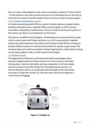
6. 5 | P a g e
Chapter 4: Object Detection
4.1 Introduction.
4.2 General object detection framework.
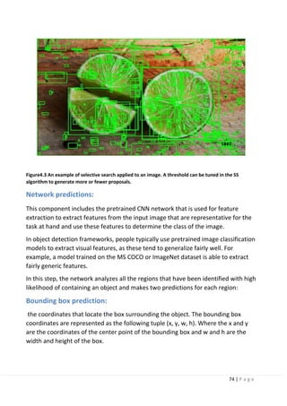
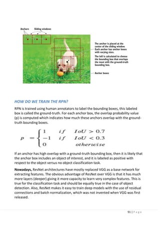
4.3 Region proposals.
4.4 Steps of how the NMS algorithm works.
4.5 Precision-Recall Curve (PR Curve).
4.6 Conclusion.
4.7 Region-Based Convolutional Neural Networks (R-CNNs) [high mAP andlow
FPS].
4.8 Fast R-CNN
4.9 Faster R-CNN
4.10 Single Shot Detection (SSD) [Detection Algorithm Used In Our Project]
4.11 Base network.
4.12 Multi-scale feature layers.
4.13 (YOLO) [high speed but low mAP][5].
4.14 What Colab Offers You?
Chapter 5: Transfer Machine Learning
5.1 Introduction.
5.1.1 Definition and why transfer learning?
5.1.2 How transfer learning works.
5.1.3 Transfer learning approaches.
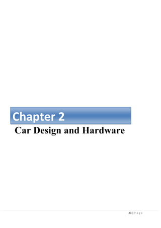
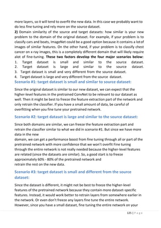
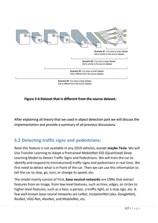
5.2 Detecting traffic signs and pedestrians.
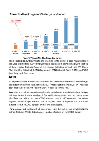
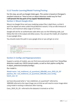
5.2.1 Model selection (most bored).
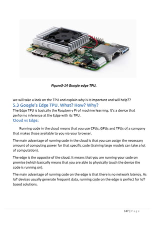
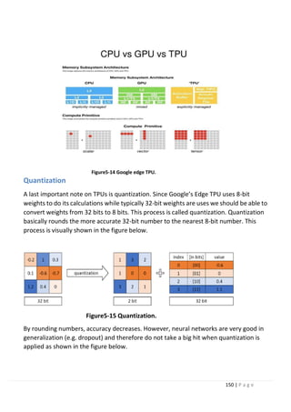
5.3 Google’s edge TPU. What? How?
why?
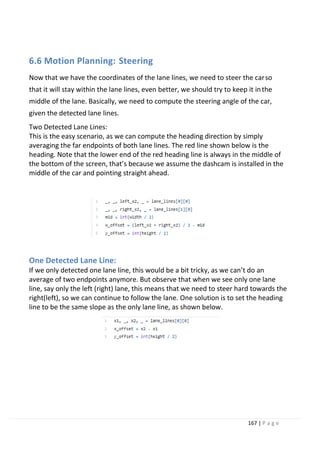
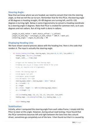
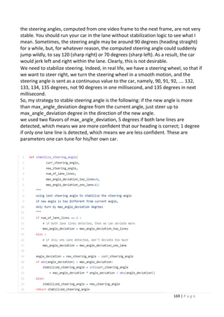
Chapter 6: Lane Keeping System
6.1 introduction
6.2 timeline of available systems

7. 6 | P a g e
6.3 current lane keeping system in market
6.4 overview of lane keeping algorithms
6.5 perception: lane Detection
6.6 motion planning: steering
6.7 lane keeping via deep learning
6.8 Google Colab for training
Chapter 7: System Integration
7.1 introduction.
7.2 connection between laptop and raspberry-pi.
7.3 connection between raspberry-pi and Arduino.
Chapter 8: software for connections
8.1 Introduction
8.2 Network
8.3 laptop to Raspberry-pi
8.4 Arduino to Raspberry-pi
References

8. 7 | P a g e
Figure 1-1 Google car.
Figure 1-2 progression of automated vehicle technologies.
Figure 2.1 System block
Figure 2.2 Top View of Chassis.
Figure 2.3 Raspberry Pi 3 model B.
Figure 2.4 Arduino Uno Board
Figure 2.5 connection of Arduino and Ultrasonic
Figure 2.6 Servo motor connection with Arduino
Figure 2.5 connection of Arduino and Ultrasonic
Figure 2.6 Turn Robot Right
Figure 2.7 Rurn Robot left
Figure 2.7 Pulse Width Modulation.
Figure 2.8 Controlling DC motor using MOSFET.
Figure 2.9 H-Bridge DC Motor Control.
Figure 2.10 L298N Motor Driver Specification.
Figure 2.11 L298N Motor Driver.
Figure 2.12 L298 control pins.
Figure 2.13 Arduino and L298N connection.
Figure 2.14 Camera module
Figure 2.15 Raspberry pi.
Figure3.1 Learning Algorithm.
Figure3-2 General Object Recognition
Figure3-3 Conventional machine learning and deep learning.
Figure3-4 Basic structure of CNN.
Figure3-5 Network structure of AlexNet and Kernels.
Figure3-6 Application of CNN to each image recognitiontask.
Figure3-7 Faster R-CNN structure.
Figure3-8 YOLO structure and examples of multiclass object detection.
Figure3-9 Fully Convolutional Network (FCN) Structure.
Figure3-10 Example of PSPNet-based Semantic Segmentation Results (cited from Reference).
Figure3-11 attention maps of CAM and Grad-CAM. (cite from reference).
Figure3-12 Regression-type Attention Branch Network. (cite from reference).
Figure3-13 Attention map-based visual explanation for self-driving.
Figure4-1 Classification and Object Detection.
Figure4-2 Low and Hight objectness score.
Figure4.3 An example of selective search applied to an image. A threshold can be tuned in the SS
algorithm to generate more or fewer proposals.
Figure4.4 Class prediction.
Figure4-5 Predictions before and after NMS.
Figure4-6 Intersection Over Union (EQU).
Figure4-7 Ground-truth and predicted box.
Figure4-8 PR Curve.
Figure4-9 Regions with CNN features.
Figure4-10 Input.
List of Figures

9. 8 | P a g e
Figure4-11 Output.
Figure4.12 Fast R-CNN.
Figure4-14 The RPN classifier predicts the objectness score which is the probability of an image
containing an object (foreground) or a background.
Figure 4-15 Anchor boxes.
Figure4-16 R-CNN, Fast R-CNN, Faster R-CNN.
Figure4-17 Comparison between R-CNN, Fast R-CNN, Faster R-CNN.
Figure4-18 SSD architecture.
Figure4.19 SSD Base Network looks at the anchor boxes to find features of a
boat. Green (solid) boxes indicate that the network has found boat features. Red (dotted) boxes indicate
no boat features.
Figure4-20 Right image - lower resolution feature maps detect larger scale objects. Left image – higher
resolution feature maps detect smaller scale objects.
Figure4-21 the accuracy with different number of feature map layers.
Figure4-22 Architecture of the multi-scale layers.
Figure4-23 YOLO splits the image into grids, predicts objects for eachgrid, then use NMS to finalize
predictions.
Figure4-24 YOLOv3 workflow.
Figure4-25 YOLOV3 Output bounding boxes.
Figure4-26 neural network architecture.
Figure4-27 Python. Figure4-28 Open CV.
Figure4-29 TensorFlow.
Figure5-1 traditional ML VS TrasferLearning.
Figure5-2 Extracted features.
Figure5-3 Feature maps.
Figure5-4 CNN Architecture Diagram, Hierarchical Feature Extraction in stages.
Figure5-5 features start to be more specific.
Figure 5-6 Dataset that is different from the source dataset.
Figure5-7 ImageNet Challenge top error.
Figure5-8 Tensorflow detection model zoo.
Figure5-9 COCO-trained models.
Figure5-10 Download pre-trained model.
Figure5-11 Part of config file the contains information about image resizer to make image suitable to
CNN make it (300x300) and architecture of box predictor CNN which include regularization and drop
out to avoid overfitting.
Figure5-11 Part of config file indicate the batch size, optimizer type and learning rate (which is vary in
this case).
Figure5-12 Part of config file the contains information about image resizer to make image suitable to
CNN make it (300x300) and architecture of box predictor CNN which include regularization and drop
out to avoid overfitting.
Figure5-13 mAP (top left), a measure of precision, keeps on increasing.
Figure5-14 Google edge TPU.
Figure5-15 Quantization.
Figure5-16 Accuracy of non-quantized model’s vs quantized models.
Figure6.1 the lane departure warning algorithm.
Figure6.2 Image in HSV Color.
Figure6.4 Hue in 0-360 degrees scale.
Figure6.3 OpenCV command.
Figure6.5 code to lift Blue out via OpenCV, and rendered mask image.
Figure6.6 OpenCV recommends.
Figure6.7 Edges of all Blue Areas.
Figure6.8 Cropped Edges.

10. 9 | P a g e
Figure6.9 CNN architecture.
Figure6.10 Method Training.
Figure6.11 Angles distribution from Data acquisition.
Figure 6.12 mount Drive to colab
Figure 6.13 python package for training.
Figure 6.14 Loading our data from drive.
Figure 6.15 train and test data.
Figure 6.16 load model.
Figure 6.17 Summary Model.
Figure6.18 Graph of training and validation loss.
Figure6.19 Result of our model on our data.
Figure7-1 Diagram for connections.
Figure7.2 Server.
Figure7.3 Client.
Figure7.4 Recording stream on connection file.
Figure7.5 Reading from connection file and Split frames on server side.
Figure7.6 Terminate connection in two sides.
Figure7.7 Operation of TCP.
Figure7.8 Graphical representation of the i2c bus.
Figure7.9 Structure of a base i2c message.
Figure7-10 I2c code in raspberry-pi.
Figure7.11 I2c code in Arduino.
Figure 8.1 Block diagram of system.
Figure 8.2 Raspberry-pi.
Figure 8.3 Then use putty or VNC to access the pi and control it remotely from its terminal.
Figure 8.4 VNC Viewer.
Figure 8.5 Putty Viewer.
Figure 8.6 Arduino board.
Figure 8.7 Access point.
Figure 8.8 Hardware schematics.

11. 10 | P a g e
N Name C
1 4 Wheel Robot Smart Car Chassis Kits Car Model with Speed
Encoder for Arduino.
1
2 Servo Motor Standard (120) 6 kg.cm Plastic Gears "FS5106B" 1
3 RS Raspberry pi Camera V2 Module Board 8MP Webcam Video. 1
4 Arduino UNO Microcontroller Development Board + USB Cable 1
5 Raspberry Pi 3 Model B+ RS Version UK Version 1
6 Micro SD 16GB-HC10 With Raspbian OS for Raspberry PI 1
7 USB Cable to Micro 1.5m 1
8 Motor Driver L298N 1
9 17 Values 1% Resistor Kit Assortment, 0 Ohm-1M Ohm 1
10 Mixed Color LEDs Size 3mm 10
11 Ultrasonic Sensor HC-04 + Ultrasonic Sensor holder 3
12 9V Battery Energizer Alkaline 1
13 9V Battery Clip with DC Plug 1
14 Lipo Battery 11.1V-5500mAh – 35C 1
15 Wires 20 cm male to male 20
16 Wires 20 cm male to female 20
17 Wires 20 cm female to female 20
18 Breadboard 400 pin 1
19 Breadboard 170 pin (White color) 1
20 Rocker switch on/off with lamp red ( KDC 2 ) 3
21 Power bank 10000 mA h 1
List of components

12. 11 | P a g e
Introduction
Chapter 1

13. 12 | P a g e
1.1 History
1930s
An early representation of the autonomous car was Norman Bell Geddes's Futurama
exhibit sponsored by General Motors at the 1939 World's Fair, which depicted electric
cars powered by circuits embedded in the roadway and controlled by radio.
1950s
In 1953, RCA Labs successfully built a
miniature car that was guided and controlled
by wires that were laid in a pattern on a
laboratory floor. The system sparked the
imagination of Leland M. Hancock, traffic
engineer in the Nebraska Department of
Roads, and of his director, L. N. Ress, state
engineer. The decision was made to
experiment with the system in actual
highway.
installations. In 1958, a full size system was successfully demonstrated by RCA Labs
and the State of Nebraska on a 400-foot strip of public highway just outside Lincoln,
Neb.
1980s
In the 1980s, a vision-guided Mercedes-Benz robotic van, designed by Ernst
Dickmanns and his team at the Bundeswehr University Munich in Munich, Germany,
achieved a speed of 39 miles per hour (63 km/h) on streets without traffic.
Subsequently, EUREKA conducted the €749 million Prometheus Project on
autonomous vehicles from 1987 to 1995.
1990s
In 1991, the United States Congress passed the ISTEA Transportation Authorization
bill, which instructed USDOT to "demonstrate an automated vehicle and highway
system by 1997." The Federal Highway Administration took on this task, first with a

14. 13 | P a g e
series of Precursor Systems Analyses and then by establishing the National
Automated Highway System Consortium (NAHSC). This cost-shared project was led
by FHWA and General Motors, with Caltrans, Delco, Parsons Brinkerhoff, Bechtel,UC-
Berkeley, Carnegie Mellon University, and Lockheed Martin as additionalpartners.
Extensive systems engineering work and research culminated in Demo '97 on I-15 in
San Diego, California, in which about 20 automated vehicles, including cars, buses,
and trucks, were demonstrated to thousands of onlookers, attracting extensive
media coverage. The demonstrations involved close-headway platooning intended to
operate in segregated traffic, as well as "free agent" vehicles intended to operate in
mixed traffic.
2000s
The US Government funded three military efforts known as Demo I (US Army), Demo
II (DARPA), and Demo III (US Army). Demo III (2001) demonstrated the ability of
unmanned ground vehicles to navigate miles of difficult off-road terrain, avoiding
obstacles such as rocks and trees. James Albus at the National Institute for Standards
and Technology provided the Real-Time Control System which is a hierarchical
control system. Not only were individual vehicles controlled (e.g. Throttle, steering,
and brake), but groups of vehicles had their movements automatically coordinated in
response to high level goals. The Park Shuttle, a driverless public road transport
system, became operational in the Netherlands in the early 2000s.In January 2006,
the United Kingdom's 'Foresight' think-tank revealed a report which predicts RFID-
tagged driverless cars on UK's roads by 2056 and the Royal Academy of Engineering
claimed that driverless trucks could be on Britain's motorways by 2019.
Autonomous vehicles have also been used in mining. Since December 2008, Rio
Tinto Alcan has been testing the Komatsu Autonomous Haulage System – the world's
first commercial autonomous mining haulage system – in the Pilbara iron ore minein
Western Australia. Rio Tinto has reported benefits in health, safety, and productivity.
In November 2011, Rio Tinto signed a deal to greatly expand its fleet of driverless
trucks. Other autonomous mining systems include Sandvik Automine’s underground
loaders and Caterpillar Inc.'s autonomous hauling.
In 2011
the Freie Universität Berlin developed two autonomous cars to drive in the inner city
traffic of Berlin in Germany. Led by the AUTONOMOS group, the two vehicles Spirit
of Berlin and made in Germany handled intercity traffic, traffic lights and
roundabouts between International Congress Centrum and Brandenburg Gate. It was
the first car licensed for autonomous driving on the streets and highways in Germany

15. 14 | P a g e
and financed by the German Federal Ministry of Education and Research.
The 2014 Mercedes S-Class has options for autonomous steering, lane keeping,
acceleration/braking, parking, accident avoidance, and driver fatigue detection, in
both city traffic and highway speeds of up to 124 miles (200 km) per hour.
Released in 2013, the 2014 Infiniti Q50 uses cameras, radar and other technology to
deliver various lane-keeping, collision avoidance and cruise control features. One
reviewer remarked, "With the Q50 managing its own speed and adjusting course, I
could sit back and simply watch, even on mildly curving highways, for three or more
miles at a stretch adding that he wasn't touching the steering wheel or pedals.
Although as of 2013, fully autonomous vehicles are not yet available to the public,
many contemporary car models have features offering limited autonomous
functionality. These include adaptive cruise control, a system that monitors
distances to adjacent vehicles in the same lane, adjusting the speed with the flow of
traffic lane which monitors the vehicle's position in the lane, and either warns the
driver when the vehicle is leaving its lane, or, less commonly, takes corrective
actions, and parking assist, which assists the driver in the task of parallel parking
In 2013
on July 12, VisLab conducted another pioneering test of autonomous vehicles,
during which a robotic vehicle drove in downtown Parma with no human control,
successfully navigating roundabouts, traffic lights, pedestrian crossings and other
common hazards.
1.2 Why autonomous car is important
1.2.1 Benefits of Self-Driving Cars
1. Fewer accidents
The leading cause of most automobile accidents today is driver error. Alcohol,
drugs, speeding, aggressive driving, over-compensation, inexperience, slow
reaction time, inattentiveness, and ignoring road conditions are all
contributing factors. Given some 40 percent of accidents can be traced to the
abuse of drugs and or alcohol, self-driving cars would practically eliminate
those accidents altogether.

16. 15 | P a g e
2. Decreased (or Eliminated) Traffic Congestion
One of the leading causes of traffic jams is selfish behavior among drivers. It
has been shown when drivers space out and allow each other to move freely
between lanes on the highway, traffic continues to flow smoothly,regardless
of the number of cars on the road.
3. Increased Highway Capacity
There is another benefit to cars traveling down the highway and
communicating with one another at regularly spaced intervals. More cars
could be on the highway simultaneously because they would need to occupy
less space on the highway
4. Enhanced Human Productivity
Currently, the time spent in our cars is largely given over to simply gettingthe
car and us from place to place. Interestingly though, even doing nothing at all
would serve to increase human productivity. Studies have shown taking short
breaks increase overall productivity.
You can also finish up a project, type a letter, monitor the progress of your
kids, schoolwork, return phone calls, take phone calls safely, textuntil your
heart’s content, read a book, or simply relax and enjoy the ride.
5. Hunting for Parking Eliminated
Self-driving cars can be programmed to let you off at the front door of your
destination, park themselves, and come back to pick you up when you
summon them. You’re freed from the task of looking for a parking space,
because the car can do it all.
6. Improved Mobility for Children, The Elderly, And the Disabled
Programming the car to pick up people, drive them to their destination and
Then Park by themselves, will change the lives of the elderly and disabled by
providing them with critical mobility.
7. Elimination of Traffic Enforcement Personnel
If every car is “plugged” into the grid and driving itself, then speeding, —
along with stop sign and red light running will be eliminated. The cop on the
side of the road measuring the speed of traffic for enforcement purposes?
Yeah, they’re gone. Cars won’t speed anymore. So, no need to Traffic
Enforcement Personnel.
8. Higher Speed Limits
Since all cars are in communication with one another, and they’re all
programmed to maintain a specific interval between one another, and they all
know when to expect each other to stop and start, the need to accommodate
human reflexes on the highway will be eliminated. Thus, cars can maintain

17. 16 | P a g e
higher average speeds.
9. Lighter, More Versatile Cars
The vast majority of the weight in today’s cars is there because of the need to
incorporate safety equipment. Steel door beams, crumple zones and the need
to build cars from steel in general relate to preparedness for accidents. Self-
driving cars will crash less often, accidents will be all but eliminated, and so
the need to build cars to withstand horrific crashes will be reduced. This
means cars can be lighter, which will make them more fuel-efficient.
1.3 What Are Autonomous and Automated Vehicles
Technological advancements are creating a continuum between conventional, fully
human-driven vehicles and automated vehicles, which partially or fully drive
themselves and which may ultimately require no driver at all. Within this continuum
are technologies that enable a vehicle to assist and make decisions for a human
driver. Such technologies include crash warning systems, adaptive cruise control
(ACC), lane keeping systems, and self-parking technology.
•Level 0 (no automation):
The driver is in complete and sole control of the primary vehicle functions (brake,
steering, throttle, and motive power) at all times, and is solely responsible for
monitoring the roadway and for safe vehicle operation.
•Level 1 (function-specific automation):
Automation at this level involves one or more specific control functions; if multiple
functions are automated, they operate independently of each other. The driver has
overall control, and is solely responsible for safe operation, but can choose to cede
limited authority over a primary control (as in ACC); the vehicle can automatically
assume limited authority over a primary control (as in electronic stability control); or
the automated system can provide added control to aid the driver in certain normal
driving or crash-imminent situations (e.g., dynamic brake support in emergencies).
•Level 2 (combined-function automation):
This level involves automation of at least two primary control functions designed to
work in unison to relieve the driver of controlling those functions. Vehicles at this
level of automation can utilize shared authority when the driver cedes active primary
control in certain limited driving situations. The driver is still responsible for
monitoring the roadway and safe operation, and is expected to be available for
control at all times and on short notice. The system can relinquish control with no
advance warning and the driver must be ready to control the vehicle safely.

18. 17 | P a g e
•Level 3 (limited self-driving automation):
Vehicles at this level of automation enable the driver to cede full control of all
safety-critical functions under certain traffic or environmental conditions, and in
those conditions to rely heavily on the vehicle to monitor for changes in those
conditions requiring transition back to driver control. The driver is expected to be
available for occasional control, but with sufficiently comfortable transition time
•Level 4 (full self-driving automation):
The vehicle is designed to perform all safety-critical driving functions and monitor
roadway conditions for an entire trip. Such a design anticipates that the driver will
provide destination or navigation input, but is not expected to be available for control
at any time during the trip. This includes both occupied and unoccupied vehicles
Our project can be considered as prototype systems of level 4 or level 5
1.4 Advanced Driver Assistance System (ADAS)
A rapid growth has been seen worldwide in the development of AdvancedDriver
Assistance Systems (ADAS) because of improvements in sensing, communicating
and computing technologies. ADAS aim to support drivers by either providing
warning to reduce risk exposure, or automating some of the control tasks to
relieve a driver from manual control of a vehicle. From an operational point of
view, such systems are a clear departure from a century of automobile
development where drivers have had control of all driving tasks at all times.
ADAS could replace some of the human driver decisions and actions with precise
machine tasks, making it possible to eliminate many of the driver errors which
could lead to accidents, and achieve more regulated and smoother vehicle
control with increased capacity and associated energy and environmental
benefits.
Autonomous ADAS systems use on-board equipment, such as ranging
sensors and machine/computer vision, to detect surrounding environment.
The main advantages of such an approach are that the system operation does not
rely on other parties and that the system can be implemented on the current road
infrastructure. Now many systems have become available on the market including

19. 18 | P a g e
Adaptive Cruise Control (ACC), Forward Collision Warning (FCW) and Lane Departure
Warning systems, and many more are under development. Currently, radar sensors
are widely used in the ADAS applications for obstacle detection. Compared with
optical or infrared sensors, the main advantage of radar sensors is that they perform
equally well during day time and night time, and in most weather conditions. Radar
can be used for target identification by making use of scattering signature
information.
It is widely used in ADAS for supporting lateral control such as lane departure
warning systems and lane keeping systems.
Currently computer vision has not yet gained a large enough acceptance in
automotive applications. Applications of computer vision depend much on the
capability of image process and pattern recognition (e.g. artificial intelligence). The
fact that computer vision is based on a passive sensory principle creates detection
difficulties in conditions with adverse lighting or in bad weather situations.
1.5 Project description
1.5.1 Auto-parking
The aim of this function is to design and implement self-parking car system that
moves a car from a traffic lane into a parking spot through accurate and realistic
steps which can be applied on a real car.
1.5.2 Adaptive cruise control (ACC)
Also radar cruise control, or traffic-aware cruise control is an optional cruise control
system for road vehicles that automatically adjusts the vehicle speed to maintain a
safe distance from vehicles ahead. It makes no use of satellite or roadside
infrastructures nor of any cooperative
support from other vehicles. Hence control is imposed based on sensor information
from on-board sensors only.
1.5.3 Lane Keeping Assist
It is a feature that in addition to Lane Departure Warning System automatically
takes steps to ensure the vehicle stays in its lane. Some vehicles combine adaptive
cruise control with lane keeping systems to provide additional safety. A lane
keeping assist mechanism can either reactively turn a vehicle back into the lane if
it starts to leave or proactively keep the vehicle in the center of the lane. Vehicle
companies often use the term "Lane Keep(ing) Assist" to refer to both reactive
Lane Keep Assist (LKA) and proactive Lane Centering Assist (LCA) but the terms are
beginning to be differentiated.
1.5.4 Lane departure

20. 19 | P a g e
Our car moves using adaptive cruise control according to distance of front vehicle
. If front vehicle is very slow and will cause our car to slow down the car will start to
check the lane next to it and then depart to the next lane in order to speed up again.
1.5.5 Indoor Positioning system
An indoor positioning system (IPS) is a system to locate objects or people inside a
building using radio waves, magnetic fields, acoustic signals, or other sensory
information collected by mobile devices. There are several commercial systems on
the market, but there is no standard for an IPS system.
IPS systems use different technologies, including distance measurement to nearby
anchor nodes (nodes with known positions, e.g., Wi-Fi access points), magnetic
positioning, dead reckoning. They either actively locate mobile devices and tags or
provide ambient location or environmental context for devices to get sensed. The
localized nature of an IPS has resulted in design fragmentation, with systems making
use of various optical, radio, or even acoustic technologies.
1.6 Related work
The appearance of driverless and automated vehicle technologies offers
enormous opportunities to remove human error from driving. It will make
driving easier, improve road safety, and ease congestion. It will also enable
drivers to choose to do other things than driving during the journey. It is
the first driverless electric car prototype built by Google to test self-driving
car project. It looks like a Smart car, with two seats and room enough for a
small amount of luggage
Figure 1-1 Google car.

21. 20 | P a g e
It operates in and around California, primarily around the Mountain View area
where Google has its headquarters.
It moves two people from one place to another without any user interaction. The car
is called by a smartphone for pick up at the user’s location with the destination set.
There is no steering wheel or manual control, simply a start button and a big red
emergency stop button. In front of the passengers there is a small screen showing the
weather and the current speed. Once the journey is done, the small screen displays a
message to remind you to take your personal belongings. Seat belts are also provided
in car to protect the passengers from the primary systems fails; plus, that emergency
stop button that passengers can hit at any time.
Powered by an electric motor with around a 100-mile range, the car uses a
combination of sensors and software to locate itself in the real world combined with
highly accurate digital maps. A GPS is used, just like the satellite navigation systems in
most cars, lasers and cameras take over to monitor the world around the car, 360-
degrees.
The software can recognize objects, people, cars, road marking, signs and traffic
lights, obeying the rules of the road. It can even detect road works and safely
navigate around them.
The new prototype has more sensors fitted to it that can see further (up to 600
feet in all directions)
The simultaneous development of a combination of technologies has brought
about this opportunity. For example, some current production vehicles now
feature adaptive cruise control and lane keeping technologies which allow the
automated control of acceleration, braking and steering for periods of time on
motorways, major A-roads and in congested traffic. Advanced emergency braking
Systems automatically apply the brakes to help drivers avoid a collision. Self-parking
systems allow a vehicle to parallel or Reverse Park completely hands free.
Developments in vehicle automation technology in the short and medium term will
move us closer to the ultimate scenario of a vehicle which is completely “driverless”.

22. 21 | P a g e
Figure 1-2 progression of automated vehicle technologies
VOLVO autonomous CAR
semi-autonomous driving features:
sensors can detect lanes and a car in front of it.
Button in the steering wheel to let the system know I want it to use
Adaptive Cruise Control with Pilot Assist.
If the XC90 lost track of the lanes, it would ask the driver to handle steering duties
with a ping and a message in the dashboard. This is called the Human-machine
interface.
BMW autonomous CAR
A new i-Series car will include forms of automated driving and
digital connectivity most likely Wi-Fi, high-definition digital
maps, sensor technology, cloud technology and artificial
intelligence.

23. 22 | P a g e
Nissan autonomous CAR
Nissan vehicles in the form of Nissan’s Safety Shield-inspired
technologies.
These technologies can monitor a nearly 360-degree view around a
vehicle
for risks, offering warnings to the driver and taking action to help
avoid crashes if necessary.

24. 23 | P a g e
Car Design and Hardware
Chapter 2

25. 24 | P a g e
2.1 System Design
Figure 2.1 System block
Figure 2.1 shows the block diagram of the system. The ultrasonic sensor, servo motor
and L298N motor driver are connected to Arduino Uno, while the Raspberry Pi Camera
was connected to the camera module port in Raspberry Pi 3. The Laptop and
Raspberry Pi are connected together via TCP protocol. The Raspberry Pi and Arduino
are connected via I2
C protocol (at chapter 6).
Raspberry Pi 3 and Arduino Uno was powered by a 5V power bank and the DC
motor powered up by a 7.2V battery. The DC motor was controlled by L298N motor
driver but Arduino send the control signal to the L298N motor driver and control the
DC motor to turn clockwise or anti clockwise. The servo motor is powered up by 5V
on board voltage regulator (red arrow) at L298N motor driver from 7.2V battery. The
ultrasonic sensor is powered up by 5V from Arduino 5V output pin.
The chassis is the body of the RC car where all the components, webcam, battery, power
bank, servo motor, Raspberry Pi 3, L298N motor driver and ultrasonic sensor are mounted on
the chassis. The chassis is two plates of were cut by laser cutting machine. We added 2 DC
motors which attached to the back wheels and Servo attached to the front wheels will use to
turn the direction of the RC car.
2.2 Chassis

26. 25 | P a g e
Figure 2.2 Top View of Chassis.
2.3 Raspberry Pi 3 Model B
Figure 2.3 Raspberry Pi 3 model B.
The Raspberry Pi is a low cost, credit-card sized computer that plugs into a computer

27. 26 | P a g e
monitor or TV, and uses a standard keyboard and mouse. It is a capable little device
that enables people of all ages to explore computing, and to learn how to program in
languages like Scratch and Python. It’s capable of doing everything you’d expect a
desktop computer to do, from browsing the internet and playing high-definition
video, to making spreadsheets, word-processing, and playing games. The Raspberry
Pi has the ability to interact with the outside world, and has been used in a wide array
of digital maker projects, from music machines and parent detectors to weather
stations and tweeting birdhouses with infra-red cameras. We want to see the
Raspberry Pi being used by kids all over the world to learn to program and understand
how computers work (1). For more details visit www.raspberrypi.org .
In our project, raspberry-pi is used to connect the camera, Arduino and laptop
together. Raspberry-pi sends the images taken by raspberry-pi camera to laptop to
make processing on it to make a decision second, then sends orders to Arduino to
control the servo and motors. The basic specification of Raspberry-pi 3 model B in the
next Table:
Raspberry Pi 3 Model B
Processor Chipset Broadcom BCM2837 64Bit ARMv7 Quad Core Processor
powered Single Board Computer running at 1250MHz
GPU VideoCore IV
Processor Speed QUAD Core @1250 MHz
RAM 1GB SDRAM @ 400 MHz
Storage MicroSD
USB 2.0 4x USB Ports
Power Draw/
voltage
2.5A @ 5V
GPIO 40 pin
Ethernet Port Yes
Wi-Fi Built in

28. 27 | P a g e
Bluetooth LE Built in
Figure 2.3 Raspberry-pi 3 model B pins layout.
2.4 Arduino Uno
Figure 2.4 Arduino Uno Board
Arduino is an open-source electronics platform based on easy-to-use hardware and
software. Arduino boards are able to read inputs - light on a sensor, a finger on a
button, or a Twitter message - and turn it into an output - activating a motor, turning
on an LED, publishing something online. You can tell your board what to do by sending
a set of instructions to the microcontroller on the board. To do so you use the Arduino
programming language (based on Wiring), and the Arduino Software (IDE), based on

29. 28 | P a g e
Processing. (2)
Arduino Uno is a microcontroller board based on 8-bit ATmega328P
microcontroller. Along with ATmega328P, it consists other components such as crystal
oscillator, serial communication, voltage regulator, etc. to support the
microcontroller. Arduino Uno has 14 digital input/output pins (out of which 6 can be
used as PWM outputs), 6 analog input pins, a USB connection, A Power barrel jack, an
ICSP header and a reset button. The next Taple contains the Technicak Specifications
on Arduino Uno:
Arduino Uno Technical Specifications
Microcontroller ATmega328P – 8 bit AVR family
microcontroller
Operating Voltage 5V
Recommended Input Voltage 7-12V
Input Voltage Limits 6-20V
Analog Input Pins 6 (A0 – A5)
Digital I/O Pins 14 (Out of which 6 provide PWM output)
DC Current on I/O Pins 40 mA
DC Current on 3.3V Pin 50 mA
Flash Memory 32 KB (0.5 KB is used for Bootloader)
SRAM 2 KB
EEPROM 1 KB
Frequency (Clock Speed) 16 MHz
In our project, Raspberry-pi send the decision to Arduino to control the DC motors,
Servo motor and Ultrasonic sensor ( figure 2.1 ) .
Arduino IDE (Integrated Development Environment) is required to program the
Arduino Uno board. For more details you can visit www.arduino.cc .

30. 29 | P a g e
2.5 Ultrasonic Sensor
Ultrasonic Sensor HC-SR04 is a sensor that can measure distance. It emits an
ultrasound at 40 000 Hz (40kHz) which travels through the air and if there is an object
or obstacle on its path It will bounce back to the module. Considering the travel time
and the speed of the sound you can calculate the distance. The configuration pin of
HC-SR04 is VCC (1), TRIG (2), ECHO (3), and GND (4). The supply voltage of VCC is
+5V and you can attach TRIG and ECHO pin to any Digital I/O in your Arduino Board.
Figure 2.5. connection of Arduino and Ultrasonic
In order to generate the ultrasound, we need to set the Trigger Pin on a High State
for 10 µs. That will send out an 8-cycle sonic burst which will travel at the speed
sound and it will be received in the Echo Pin. The Echo Pin will output the time in
microseconds the sound wave traveled. For example, if the object is 20 cm away from
the sensor, and the speed of the sound is 340 m/s or 0.034 cm/µs the sound wave will
need to travel about 588 microseconds. But what you will get from the Echo pin will
be double that number because the sound wave needs to travel forward and bounce
backward. So, in order to get the distance in cm we need to multiply the received
travel time value from the echo pin by 0.034 and divide it by2. The Arduino code is
written below:
ultrasound

31. 30 | P a g e
Results: After uploading the code, display the data with Serial Monitor. Now try to
give an object in front of the sensor and see the measurement.

32. 31 | P a g e
2.6 servo Motor
Servo motors are great devices that can turn to a specified position. they have a servo
arm that can turn 180 degrees. Using the Arduino, we can tell a servo to go to a
specified position and it will go there.
We used Servo motors in our project to control the steering of the car.
A servo motor has everything built in: a motor, a feedback circuit, and a motor driver.
It just needs one power line, one ground, and one control pin.
Figure 2.6 Servo motor connection with Arduino
Following are the steps to connect a servo motor to the Arduino:
1. The servo motor has a female connector with three pins. The darkest or even
black one is usually the ground. Connect this to the Arduino GND.
2. Connect the power cable that in all standards should be red to 5V on the
Arduino.
3. Connect the remaining line on the servo connector to a digital pin on the
Arduino.

33. 32 | P a g e
The following code will turn a servo motor to 0 degrees, wait 1 second, then turn it to
90, wait one more second, turn it to 180, and then go back.
The servo motor used to turn the robot right or left
Arduino. Depending on the angle from
Figure 2.6 Turn Robot Right Figure 2.6 Turn Robot left

34. 33 | P a g e
2.7 L298N Dual H-Bridge Motor Driver and DC Motors
DC Motor:
A DC motor (Direct Current motor) is the most common type of motor. DC motors
normally have just two leads, one positive and one negative. If you connect these
two leads directly to a battery, the motor will rotate. If you switch the leads, the
motor will rotate in the opposite direction.
PWM DC Motor Control:
PWM, or pulse width modulation is a technique which allows us to adjust the average
value of the voltage that’s going to the electronic device by turning on and off the
power at a fast rate. The average voltage depends on the duty cycle, or the amount
of time the signal is ON versus the amount of time the signal is OFF in a single period
of time. We can control the speed of the DC motor by simply controlling the input
voltage to the motor and the most common method of doing that is by using PWM
signal.
So, depending on the size of the motor, we can simply connect an Arduino PWM
output to the base of transistor or the gate of a MOSFET and control the speed of the
motor by controlling the PWM output. The low power Arduino PWM signal switches
on and off the gate at the MOSFET through
which the high-power motor is driven.
Note that Arduino GND and the motor
power supply GND should be connected
Figure 2.7 Pulse Width Modulation.

35. 34 | P a g e
Figure 2.8 Controlling DC motor using MOSFET.
Figure 2.9 H-Bridge DC Motor Control.

36. 35 | P a g e
H-Bridge DC Motor Control:
For controlling the rotation direction, we just need to inverse the direction of the
current flow through the motor, and the most common method of doing that is by
using an H-Bridge. An H-Bridge circuit contains four switching elements, transistors or
MOSFETs, with the motor at the center forming an H-like configuration. Byactivating
two particular switches at the same time we can change the direction of the current
flow, thus change the rotation direction of the motor.
So, if we combine these two methods, the PWM and the H-Bridge, we can have a
complete control over the DC motor. There are many DC motor drivers that have
these features and the L298N is one of them.
L298N Driver:
The L298N is a dual H-Bridge motor driver which allows speed and direction control
of two DC motors at the same time. The module can drive DC motors that have
voltages between 5 and 35V, with a peak current up to 2A.
L298N module has two screw terminal blocks for the motor A and B, and another
screw terminal block for the Ground pin, the VCC for motor and a 5V pin which can
either be an input or output. This depends on the voltage used at the motors VCC.
The module have an onboard 5V regulator which is either enabled or disabled using
a jumper. If the motor supply voltage is up to 12V we can enable the 5V regulator
and the 5V pin can be used as output, for example for powering our Arduino board.
But if the motor voltage is greater than 12V we must disconnect the jumperbecause
those voltages will cause damage to the onboard 5V regulator. In this case the 5V
pin will be used as input as we need connect it to a 5V power supply in order the IC
to work properly. But this IC makes a voltage drop of about 2V.

37. 36 | P a g e
L298N Motor Driver Specification
Operating Voltage 5V ~ 35V
Logic Power Output Vss 5V ~ 7V
Logical Current 0 ~36mA
Drive Current 2A (Max single bridge)
Max Power 25W
Controlling Level Low: -0.3V ~ 1.5V
High: 2.3V ~ Vss
Enable Signal Low: -0.3V ~ 1.5V
High: 2.3V ~ Vss
Table 2.10 L298N Motor Driver Specification.
Figure 2.11 L298N Motor Driver.
So, for example, if we use a 12V power supply, the voltage at motors terminals
will be about 10V, which means that we won’t be able to get the maximum speed
out of our 12V DC motor.

38. 37 | P a g e
Next are the logic control inputs. The Enable A and Enable B pins are used for enabling
and controlling the speed of the motor. If a jumper is present on this pin, the motor
will be enabled and work at
maximum speed, and if we
remove the jumper we can
connect a PWM input to this
pin and in that way control the
speed of the motor. If we
connect this pin to a Ground
Figure 2.12 L298 control pins.
the motor will be disabled.
The Input 1 and Input 2 pins are used for controlling the rotation direction of the
motor A, and the inputs 3 and 4 for the motor B. Using these pins, we actually
control the switches of the H-Bridge inside the L298N IC. If input 1 is LOW and input 2
is HIGH the motor will move forward, and if input 1 is HIGH and input 2 is LOW the
motor will move backward. In case both inputs are same, either LOW or HIGH the
motor will stop. The same applies for the inputs 3 and 4 and the motor B.
Arduino and L298N
For example, we will control
the speed of the motor using a
potentiometer and change the
rotation direction using a push
button.
Figure 2.13 Arduino and L298N connection

39. 38 | P a g e
Here’s the Arduino code:
Figure2-14 Arduino code.
we check whether we have pressed the button, and if that’s true, we will change the
rotation direction of the motor by setting the Input 1 and Input 2 states inversely. The
push button will work as toggle button and each time we press it, it will change the
rotation direction of the motor.

40. 39 | P a g e
2.8 the Camera Module
The Raspberry Pi Camera Module is used to take pictures, record video, and apply
image effects. In our project we used it for computer vision to detect the lanes of the
road and detect the signs and cars.
Figure 2.14 Camera module. Figure 2.15 Raspberry pi.
Camera.
Figure 2.16 Camera connection with raspberry.
The Python picamera library allows us to control the Camera Module and create
amazing projects. A small example to use the camera on raspberry pi that allow us
to start camera preview for 5 seconds:

41. 40 | P a g e
You can go to system integration chapter to see the usage of the camera in our
project, also you can visit raspberrypi website to see many projects on the raspberry
pi camera.

42. 41 | P a g e
Deep Learning
Chapter 3

43. 42 | P a g e
3.2 Introduction:
1) Grew out of work in AI
2) New capability for computers
Examples:
1) Database mining
Large datasets from growth of automation/web.
E.g., Web click data, medical records, biology, engineering
2) Applications can’t program by hand.
E.g., Autonomous helicopter, handwriting recognition, most of Natural
Language Processing (NLP), Computer Vision.
3.2 What is machine learning:
Arthur Samuel (1959):
Machine Learning: Field of study that gives computers the ability to learn
without being explicitly programmed.
Tom Mitchell (1998):
Well-posed Learning Problem: A computer program is said to learn from
experience E with respect to some task T and some performance measure P, if
its performance on T, as measured by P, improves with experience E.
3.2.3 Machine learning algorithms:
1) Supervised learning
2) Unsupervised learning
Others:
Reinforcement learning, recommender systems.

44. 43 | P a g e
Training Set
Learning Algorithm
Input
h
Output
Supervised Learning: (Given the “right answer”)
for each example in the data.
Regression: Predict continuous valuedoutput.
Classification: Discrete valued output (0 or1).
Figure3.1 Learning Algorithm.
3.2.4 Classification:
Multiclass classification:
1) Email foldering, tagging: Work, Friends, Family, Hobby.
2)Medical diagrams: Not ill, Cold, Flu.
3)Weather: Sunny, Cloudy, Rain, Snow.

45. 44 | P a g e
x2
Binary classification:
Multi-class classification:
x1
Regularization
x1

46. 45 | P a g e
3.2.3 The problem of overfitting:
Overfitting: If we have too many features, the learned hypothesis may fit the
training set very well but fail to generalize to new examples (predict prices on new
examples).
3.3 Representation of Neural Networks:
What is this?
You see this:
But the camera sees this:

47. 46 | P a g e
Cars
Not a car
Learning
Algorithm
pixel2
3.3Computer Vision:
Car detection
Testing:
What is this?
pixel1

48. 47 | P a g e
pixel 1 intensity
pixel 2 intensity
pixel 2500 intensity
50 x 50-pixel images→ 2500 pixels, (7500 if RGB)
Quadratic features
( ): ≈3 million features
That’s why we need neural network.
Neural Network
Multi-class classification:
Pedestri Car Motorcy Truck

49. 48 | P a g e
Multiple output units: One-vs-all.
when pedestrian when car when motorcycle
3.4 Training a neural network:
1) Pick a network architecture (connectivity pattern between neurons).
No. of input units: Dimension of features.
No. output units: Number of classes.

50. 49 | P a g e
Reasonable default: 1 hidden layer, or if >1 hidden layer, have same no. of hidden
units in every layer (usually the more the better)
2)Randomly initialize weights.
3)Implement forward propagation to get h(theta) for any x(i).
4)Implement code to compute cost function J(theta).
5)Implement backprop to compute partial derivatives.
3.4.1 Advice for applying machine learning:
Debugging a learning algorithm:
Suppose you have implemented regularized linear regression to predict housing
prices. However, when you test your hypothesis in a new set of houses, you find that
it makes unacceptably large errors in its prediction. What should you try next?
1)Get more training examples
2)Try smaller sets of features
3)Try getting additional features
4)Try adding polynomialfeatures
5)Try decreasing lambda
6)Try increasing lambda
3.4.2 Neural networks and overfitting:
“Small” neural network
(fewer parameters; more prone to underfitting)
Computationally cheaper
“Large” neural network
(more parameters; more prone to overfitting)

51. 50 | P a g e
Computationally more expensive.
Use regularization (lambda) to address overfitting.
3.5 Neural Networks and Introduction to Deep Learning:
Deep learning is a set of learning methods attempting to model data with
complex architectures combining different non-linear transformations. The
elementary bricks of deep learning are the neural networks, that are combined
to form the deep neural networks.
These techniques have enabled significant progress in the fields of sound
and image processing, including facial recognition, speech recognition, computer
vision, automated language processing, text classification (for example
spam recognition). Potential applications are very numerous. A spectacularly
example is the AlphaGo program, which learned to play the go game by the
deep learning method, and beated the world champion in 2016.
There exist several types of architectures for neural networks:
• The multilayer perceptrons: that are the oldest and simplest ones.
• The Convolutional Neural Networks (CNN): particularly adapted forimage
processing.
• The recurrent neural networks: used for sequential data such as textor
times series.
They are based on deep cascade of layers. They need clever stochastic
optimization algorithms, and initialization, and also a clever choice of the

52. 51 | P a g e
structure. They lead to very impressive results, although very few theoretical
foundations are available till now.
Neural networks:
An artificial neural network is an application, nonlinear with respect to its
parameters θ that associates to an entry x an output y = f(x; θ). For the
sake of simplicity, we assume that y is unidimensional, but it could also be
multidimensional. This application f has a particular form that we will precise.
The neural networks can be used for regression or classification. As usual in
statistical learning, the parameters θ are estimated from a learning sample. The
function to minimize is not convex, leading to local minimizers. The success
of the method came from a universal approximation theorem due to Cybenko
(1989) and Horik (1991). Moreover, Le Cun (1986) proposed an efficient way
to compute the gradient of a neural network, called backpropagation of the
gradient, that allows to obtain a local minimizer of the quadratic criterion
easily.
Artificial Neuron:
An artificial neuron is a function fj of the input x = (x1; : : : ; xd) weighted
by a vector of connection weights wj = (wj;1; : : : ; wj;d), completed by a
neuron bias bj, and associated to an activation function φ, namely
yj = fj(x) = φ(hwj; xi + bj):
Several activation functions can be considered.
Convolutional neural networks:
For some types of data, especially for images, multilayer perceptrons are not
well adapted. Indeed, they are defined for vectors as input data, hence, to apply
them to images, we should transform the images into vectors, losing by the
way the spatial information contained in the images, such as forms. Before the
development of deep learning for computer vision, learning was based on the
extraction of variables of interest, called features, but these methods need a lot
of experience for image processing. The convolutional neural networks (CNN)
introduced by LeCun have revolutionized image processing,and
removed the manual extraction of features. CNN act directly on matrices,
or even on tensors for images with three RGB color channels. CNN are
now
widely used for image classification, image segmentation, object recognition,
face recognition.
Layers in a CNN:
A Convolutional Neural Network is composed by several kinds of layers,

53. 52 | P a g e
that are described in this section: convolutional layers, pooling layers and
fully connected layers. After several convolution and pooling layers, the CNN
generally ends with several fully connected layers. The tensor that we have at the
output of these layers is transformed into a vector and then we add several
perceptron layers .Deep learning-based image recognition for autonomous
driving Various image recognition tasks were handled in the image recognition
field prior to 2010 by combining image local features manually designed by
researchers (called handcrafted features) and machine learning method.
After entering the 2010, However, many image recognition methods that use
deep learning have been proposed.
The image recognition methods using deep learning are far superior to the
methods used prior to the appearance of deep learning in general object
recognition competitions. Hence, this paper will explain how deep learning is
applied to the field of image recognition, and will also explain the latest trends of
deep learning-based autonomous driving.
In the late 1990s, it became possible to process a large amount of data at high speed
with the evolution of general-purpose computers. The mainstream method was to
extract a feature vector (called the image local features) from the image and apply a
machine learning method to perform image recognition. Supervised machine
learning requires a large amount of class-labeled training samples, but it does not
require researchers to design some rules as in the case of rule-based methods. So,
versatile image recognition can be realized. In the 2000 era, handcrafted features
such as scale-invariant feature transform (SIFT) and histogram of oriented gradients
(HOG) as image local features, designed based on the knowledge of researchers,
have been actively researched. By combining the image local features with machine
learning, practical applications of image recognition technology have advanced, as
represented by face detection. Next, in the late 2010s, deep learning to perform
feature extraction process through learning has come under the spotlight. A
handcrafted feature is not necessarily optimal because it extracts and expresses
feature values using a designed algorithm based on the knowledge of researchers.
Deep learning is an approach that can automate the feature extraction process and
is effective for image recognition. Deep learning has accomplished. M pressive
results in the general object recognition competitions, and the use of image
recognition required for autonomous driving (such as object detection and semantic
segmentation) is in progress. This paper explains how deep learning is applied to
each task in image recognition and how it is solved, and describes the trend of deep
learning-based autonomous driving and related problems.

54. 53 | P a g e
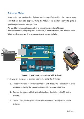
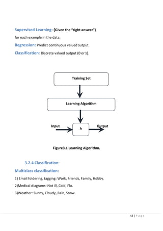
3.6 Problem setting in image recognition:
In conventional machine learning (here, it is defined as a method prior to the time
when deep learning gained attention), it is difficult to directly solve general object
recognition tasks from the input image. This problem can be solved by distinguishing
the tasks of image identification, image classification, object detection, scene
understanding, and specific object recognition. Definitions of each task
and approaches to each task are described below.
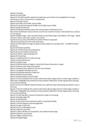
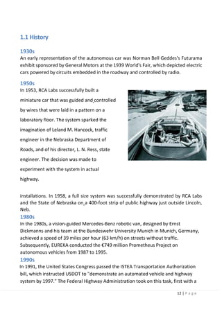
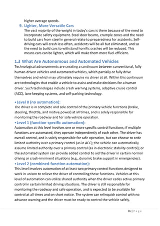
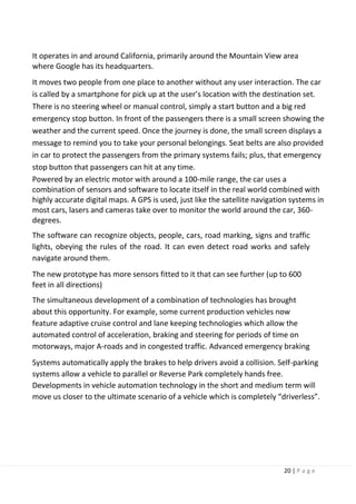
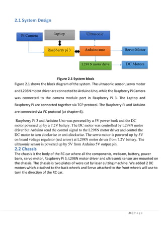
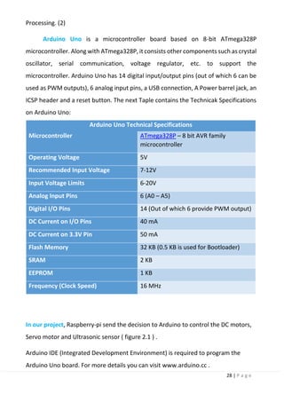
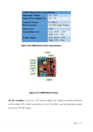
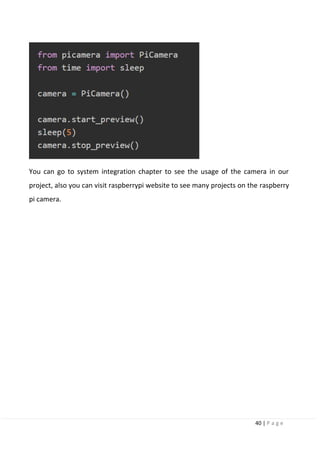
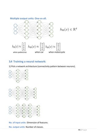
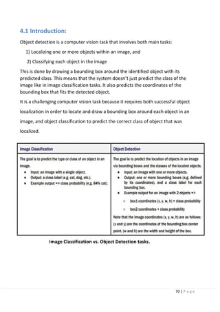
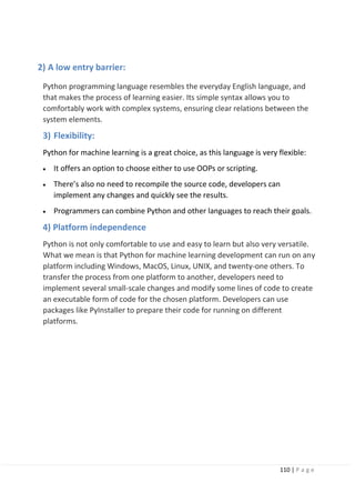
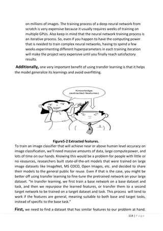
Image verification:
Image verification is a problem to check whether the object in the
image is the same as the reference pattern. In image verification, the
distance between the feature vector of the reference pattern and the
feature vector of the input image is calculated. If the distance value is less
than a certain value, the images are determined as identical, and if the
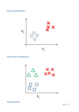
value is more, it is determined otherwise. Fingerprint, face, and person
identification relates to tasks in which it is required to determine
whether an actual person is another person. In deep learning, the problem
of person identification is solved by designing a loss function (triplet loss
function) that calculates the value of distance between two images of the
same person as small, and the value of distance with another person's
image as large [1].
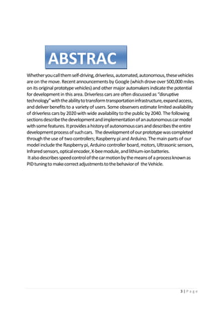
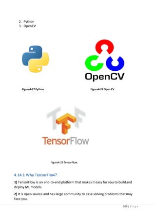
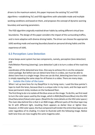
Figure3-2 General Object Recognition.

55. 54 | P a g e
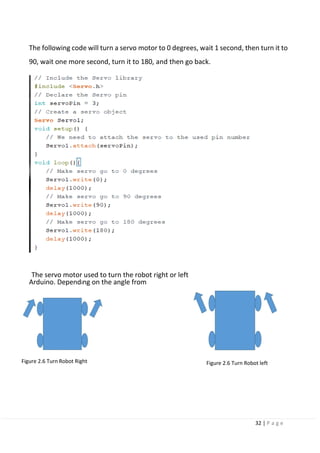
Object detection:
Object detection is the problem of finding the location of an object of a certain
category in the image. Practical face detection and pedestrian detection are
included in this task. Face detection uses a combination of Haar-like features [2]
and AdaBoost, and pedestrian detection uses HOG features [3] and support vector
machine (SVM). In conventional machine learning, object detection is achieved by
training 2-class classifiers corresponding to a certain category and raster scanning
in the image. In deep learning-based object detection, multiclass object detection
targeting several categories can be achieved with one network.
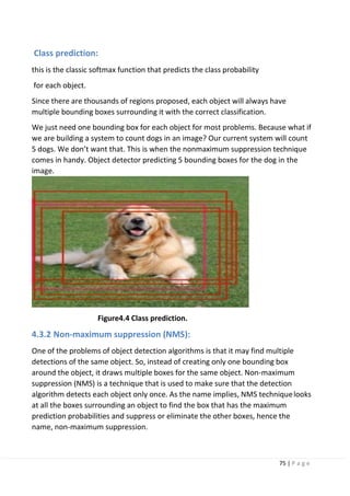
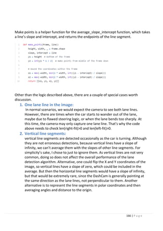
Image classification:
Image classification is a problem to find out the category to which an object in an
image belongs to, among predefined categories. In the conventional machine
learning, an approach called bag-of-features (BoF) has been used: a vector quantifies
the image local features and expresses the features of the whole image as a
histogram. Yet, deep learning is well-suited to the image classification task, and
became popular in 2015 by achieving an accuracy exceeding human recognition
performance in the 1000-class image classification task.
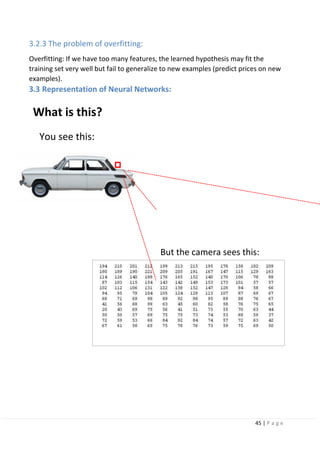
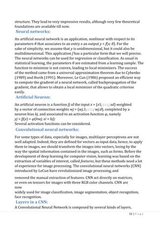
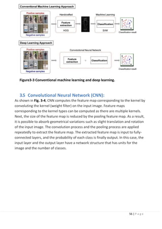
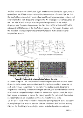
3.7 Convolutional Neural Network (CNN):
CNN computes the feature map corresponding to the kernel by convoluting the
kernel (weight filter) on the input image. Feature maps corresponding to the kernel
types can be computed as there are multiple kernels. Next, the size of the feature
map is reduced by the pooling feature map. As a result, it is possible to absorb
geometrical variations such as slight translation and rotation of the input image.
The convolution process and the pooling process are applied repeatedly to extract
the feature map. The extracted feature map is input to fully connected layers, and
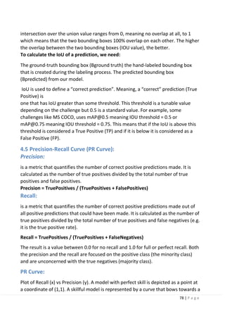
the probability of each class is finally output. In this case, the input layer and the
output layer have a network structure that has units for the image and the number
of classes. Training of CNN is achieved by updating the parameters of the network by
the backpropagation method. The parameters in CNN refer to the kernel of the
convolutional layer and the weights of all coupled layers. The process flow of the
backpropagation method is shown:

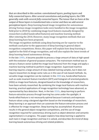
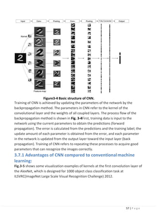
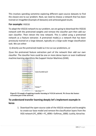
56. 55 | P a g e
First,training data is input to the network using the current parameters to obtain
the predictions (forward propagation). The error is calculated from the predictions
and the training label; the update amount of each parameter is obtained from the
error, and each parameter in the network is updated from the output layer toward
the input layer (back propagation). Training of CNN refers to repeating these
processes to acquire good parameters that can recognize the images correctly.
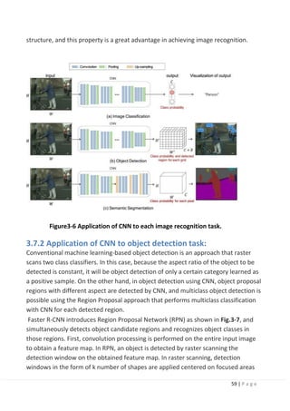
Scene understanding (semantic segmentation):
Scene understanding is the problem of understanding the scene structure in an
image. Above all, semantic segmentation that finds object categories in each pixel in
an image has been considered difficult to solve using conventional machine learning.
Therefore, it has been regarded as one of the ultimate problems of computer vision,
but it has been shown that it is a problem that can be solved by applying deep
learning.
Specific object recognition:
Specific object recognition is the problem of finding a specific object. By giving
attributes to objects with proper nouns, specific object recognition is defined as a
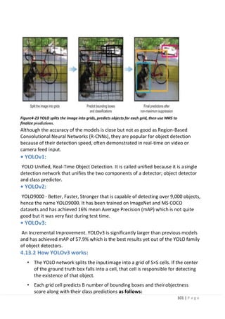
subtask of the general object recognition problem. Specific object recognition is
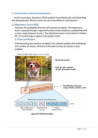
achieved by detecting feature points using SIFT from images, and a voting process
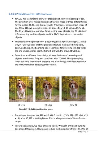
based on the calculation of distance from feature points of reference patterns.
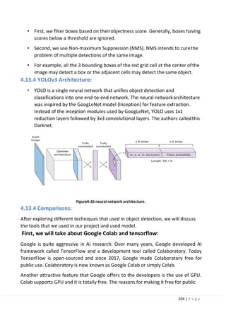
Machine learning is not used here directly here, but the learned invariant feature
transform (LIFT) proposed in 2016 achieved an improvement in performance by
learning and replacing each process in SIFT through deep learning.
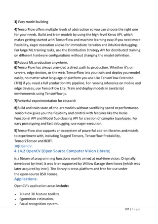
3.4 Deep learning-based image recognition:
Image recognition prior to deep learning is not always optimal because image
features are extracted and expressed using an algorithm designed based on the
knowledge of researchers, which is called a handcrafted feature. Convolutional
neural network (CNN) [7]), which is one type of deep learning, is an approach for
learning classification and feature extraction from training samples, as shown in This
chapter describes CNN, focuses on object detection and scene understanding
(semantic segmentation), and describes its application to image recognition and its
trends.

57. 56 | P a g e
Figure3-3 Conventional machine learning and deep learning.
3.5 Convolutional Neural Network (CNN):
As shown in Fig. 3-4, CNN computes the feature map corresponding to the kernel by
convoluting the kernel (weight filter) on the input image. Feature maps
corresponding to the kernel types can be computed as there are multiple kernels.
Next, the size of the feature map is reduced by the pooling feature map. As a result,
it is possible to absorb geometrical variations such as slight translation and rotation
of the input image. The convolution process and the pooling process are applied
repeatedly to extract the feature map. The extracted feature map is input to fully-
connected layers, and the probability of each class is finally output. In this case, the
input layer and the output layer have a network structure that has units for the
image and the number of classes.

58. 57 | P a g e
Figure3-4 Basic structure of CNN.
Training of CNN is achieved by updating the parameters of the network by the
backpropagation method. The parameters in CNN refer to the kernel of the
convolutional layer and the weights of all coupled layers. The process flow of the
backpropagation method is shown in Fig. 3-4First, training data is input to the
network using the current parameters to obtain the predictions (forward
propagation). The error is calculated from the predictions and the training label; the
update amount of each parameter is obtained from the error, and each parameter
in the network is updated from the output layer toward the input layer (back
propagation). Training of CNN refers to repeating these processes to acquire good
parameters that can recognize the images correctly.
3.7.1 Advantages of CNN compared to conventionalmachine
learning:
Fig.3-5 shows some visualization examples of kernels at the first convolution layer of
the AlexNet, which is designed for 1000 object class classification task at
ILSVRC(ImageNet Large Scale Visual Recognition Challenge) 2012.

59. 58 | P a g e
AlexNet consists of five convolution layers and three fully-connected layers, whose
output layer has 10,000 units corresponding to the number of classes. We see that
the AlexNet has automatically acquired various filters that extract edge, texture, and
color information with directional components. We investigated the effectiveness of
the CNN filter as a local image feature by comparing the HOG in the human
detection task. The detection miss rate for CNN filters is 3%, while the HOG is 8%.
Although the CNN kernels of the AlexNet not trained for the human detection task,
the detection accuracy improved over the HOG feature that is the traditional
handcrafted feature.
Figure3-5 Network structure of AlexNet and Kernels.
As shown in Fig.3-6, CNN can perform not only image classification but also object
detection and semantic segmentation by designing the output layer according to
each task of image recognition. For example, if the output layer is designed to
output class probability and detection region for each grid, it will become a network
structure that can perform object detection. In semantic segmentation, the output
layer should be designed to output the class probability for each pixel. Convolution
and pooling layers can be used as common modules for these tasks.
On the other hand, in the conventional machine learning method, it was necessary
to design image local features for each task and combine it with machine learning.
CNN has the flexibility to be applied to various tasks by changing the network

60. 59 | P a g e
structure, and this property is a great advantage in achieving image recognition.
Figure3-6 Application of CNN to each image recognition task.
3.7.2 Application of CNN to object detection task:
Conventional machine learning-based object detection is an approach that raster
scans two class classifiers. In this case, because the aspect ratio of the object to be
detected is constant, it will be object detection of only a certain category learned as
a positive sample. On the other hand, in object detection using CNN, object proposal
regions with different aspect are detected by CNN, and multiclass object detection is
possible using the Region Proposal approach that performs multiclass classification
with CNN for each detected region.
Faster R-CNN introduces Region Proposal Network (RPN) as shown in Fig.3-7, and
simultaneously detects object candidate regions and recognizes object classes in
those regions. First, convolution processing is performed on the entire input image
to obtain a feature map. In RPN, an object is detected by raster scanning the
detection window on the obtained feature map. In raster scanning, detection
windows in the form of k number of shapes are applied centered on focused areas

61. 60 | P a g e
known as anchor. The region specified by the anchor is input to RPN, and the score
of object likeness and the detected coordinates on the input image are output. In
addition, the region specified by the anchor is also input to another all-connected
network, and object recognition is performed when it is determined to be an object
by RPN. Therefore, the unit of the output layer is the number obtained by addingthe
number of classes and ((x, y, w, h) × number of classes) to one rectangle. These
Region Proposal methods have made it possible to detect multiple classes of objects
with different aspect ratios.
Figure3-7 Faster R-CNN structure.
In 2016, the single-shot method was proposed as a new multiclass object detection
approach. This is a method to detect multiple objects only by giving the whole image
to CNN without raster scanning the image. YOLO (You Only Look Once) is a
representative method in which an object rectangle and an object category is output
for each local region divided by a 7 × 7 grid, as shown in Fig3-7. First, feature maps
are generated through convolution and pooling of input images. The position (i, j) of
each channel of the obtained feature map (7 × 7 × 1024) is a structure that becomes
a region feature corresponding to the grid (i, j) of the input image, and this feature
map is input to fully connected layers. The output values obtained through fully
connected layers are the score (20 categories) of the object category at each grid
position and the position, size, and reliability of the two object rectangles.
Therefore, the unit of the output layer is the number (1470) in which the position,
size, and reliability ((x, y, w, h, reliability) × 2) of two object rectangles is added to
the number of categories (20 categories) and multiplied with the number of grids (7
× 7). In YOLO, it is not necessary to detect object region candidates such as Faster R-
CNN; therefore, object detection can be performed in real time. Fig.3-8 shows an

62. 61 | P a g e
example of YOLO-based multiclass object detection.
Figure3-8 YOLO structure and examples of multiclass object detection.
3.7.3 Application of CNN to semantic segmentation:
Semantic segmentation is a difficult task and has been studied for many years in the
field of computer vision. However, as with other tasks, deep learning-based methods
have been proposed and achieved much higher performance than conventional
machine learning methods. Fully convolutional network (FCN) is a method that
enables end-to-end learning and can obtain segmentation results using only CNN.
The structure of FCN is shown in Fig.3-9. The FCN has a network structure that does
not have a fully-connected layer.
The size of the generated feature map is reduced by repeatedly performing the
convolutional layer and the pooling layer on the input image. To make it the same
size as the original image, the feature map is enlarged 32 times in the final layer, and

63. 62 | P a g e
convolution processing is performed. This is called deconvolution. The final layer
outputs the probability map of each class. The probability map is trained so that the
probability of the class in each pixel is obtained, and the unit of output of the end-
to-end segmentation model is (w × h × number of classes). Generally, the feature
map of the middle layer of CNN captures more detailed information as it is closer to
the input layer, and the pooling process integrates these pieces of information,
resulting in the loss of detailed information. When this feature map is expanded,
coarse segmentation results are obtained. Therefore, high accuracy is achieved by
integrating and using the feature map of the middle layer. Additionally, FCN
performs processing to integrate feature maps in the middle of the network.
Convolution process is performed by connecting mid-feature maps in the channel
direction, and segmentation results of the same size as the original image are
output.
Figure3-9 Fully Convolutional Network (FCN) Structure.
When expanding the feature map obtained on the encoder side, PSPNet can capture
information of different scales by using the Pyramid Pooling Module, which expands
at multiple scales. The Pyramid Pooling Module is used to pool feature maps with 1
× 1, 2 × 2, 3 × 3, 3 × 6 × 6 in which the vertical and horizontal sizes ofthe original
image are reduced to 1/8, respectively, on the encoder side. Then, convolution
process is performed on each feature map.
Next, the convolution process is performed and probability maps of each class are
output after expanding and linking feature maps to the same size. PSPNet is the
method that won in the “Scene parsing” category of ILSVRC held in 2016. Also, high
accuracy has been achieved with the Cityscapes Dataset taken with a dashboard
camera. Fig3-10 shows the result of PSPNet-based semantic segmentation.

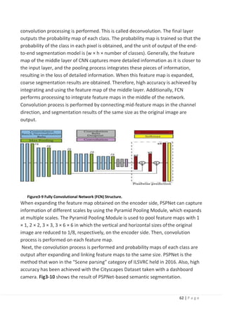
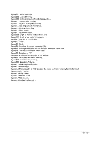
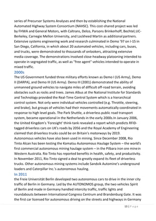
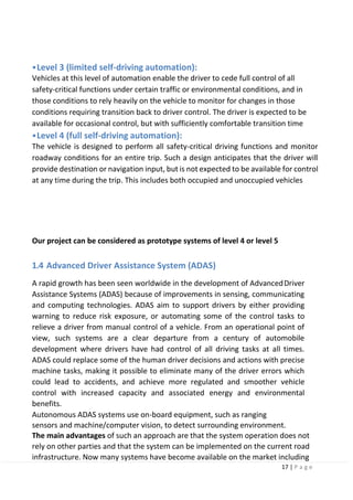
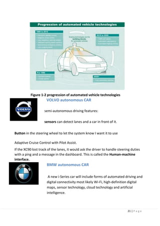
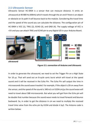
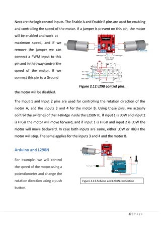
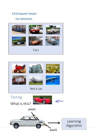
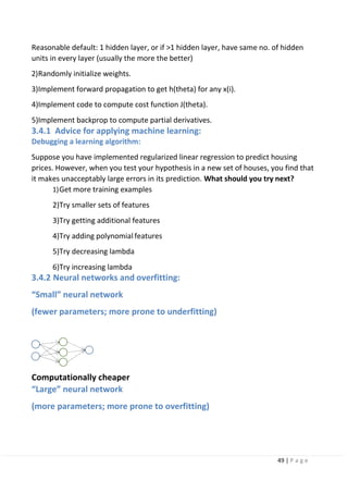
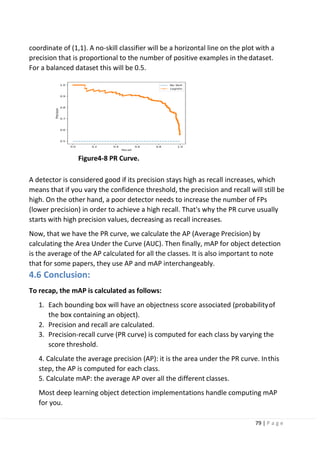
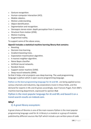
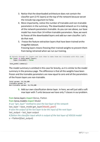
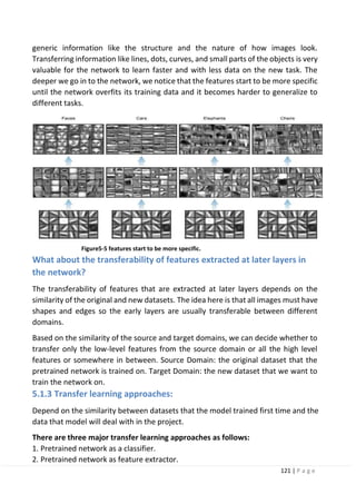
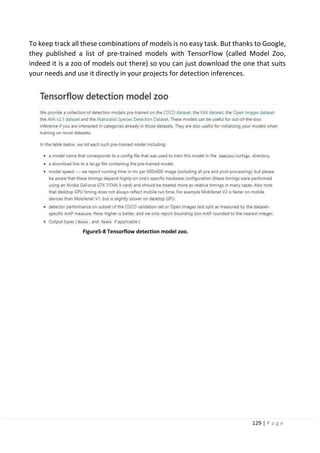
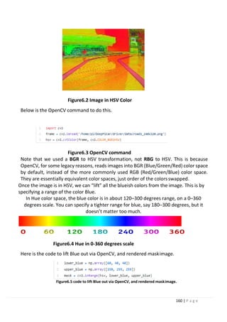
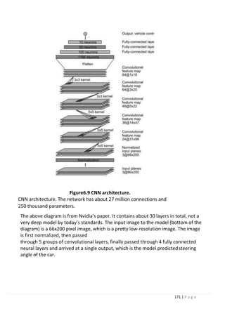
64. 63 | P a g e
Figure3-10 Example of PSPNet-based Semantic Segmentation Results (cited
from Reference [11]).
3.7.4 CNN for ADAS application:
The machine learning technique is applicable to use for system intelligence
implementation in ADAS(Advanced Driving Assistance System). In ADAS, it is to
facilitate the driver with the latest surrounding information obtained by sonar,
radar, and cameras. Although ADAS typically utilizes radar and sonar for long-range
detection, CNN-based systems can recently play a significant role in pedestrian
detection, lane detection, and redundant object detection at moderate distances.
For autonomous driving, the core component can be categorized into three
categories, namely perception, planning, and control. Perception refers to the
understanding of the environment, such as where obstacles located, detection of
road signs/marking, and categorizing objects by their semantic labels such as
pedestrians, bikes, and vehicles.
Localization refers to the ability of the autonomous vehicle to determine its position
in the environment. Planning refers to the process of making decisions in order to
achieve the vehicle's goals, typically to bring the vehicle from a start location to a
goal location while avoiding obstacles and optimizing the trajectory. Finally, the
control refers to the vehicle's ability to execute the planned actions. CNN-based
object detection is suitable for the perception because it can handle the multi-class
objects. Also, semantic segmentation is useful information for making decisions in

65. 64 | P a g e
planning to avoid the obstacles by referring to pixels categorized as road.
3.8 Deep learning-based autonomous driving:
This chapter introduces end-to-end learning that can infer the control value of the
vehicle directly from the input image as the use of deep learning for autonomous
driving, and describes visual explanation of judgment grounds that is the problem of
deep learning models and future challenges.
3.8.1 End-to-end learning-based autonomous driving:
In most of the research on autonomous driving, the environment around the vehicle
is understood using a dashboard camera and Light Detection and Ranging (LiDAR),
appropriate traveling position is determined by motion planning, and the control
value of the vehicle is determined. Autonomous driving based on these three
processes is common, and deep learning-based object detection and semantic
segmentation introduced in Chapter 3 are beginning to be used to understand the
surrounding environment. On the other hand, with the progress in CNN research,
end-to-end learning-based method has been proposed that can infer the control
value of the vehicle directly from the input image.
In these methods, network is trained by using the images of the dashboard camera
when driven by a person, and the vehicle control value corresponding to each frame
as learning data. End-to-end learning-based autonomous driving control has the
advantage that the system configuration is simplified because CNN learns
automatically and consistently without explicit understanding of the surrounding
environment and motion planning.
To this end, Bojarski et al. proposed an end-to-end learning method for autonomous
driving, which input dash-board camera images into a CNN and outputs steering
angle directory. Started by this work, several works have been conducted: a method
considering temporal structure of a dash-board camera video or a method to train
CNN by using a driving simulator and use the trained network to control vehicle
under real environment. These methods basically control only steering angle and
throttle (i.e., accelerator and brake) is controlled by human.
According to autonomous driving model in Reference , it infers not only the steering
but also the throttle as the control value of the vehicle. The network structure is
composed of five layers of convolutional layers through pooling process and three
layers of fully-connected layers. In addition, the inference is made in consideration
of one's own state by giving the vehicle speed to the fully-connected layer in
addition to the dashboard images, since it is necessary to infer the change of speed

66. 65 | P a g e
in one's own vehicle for throttle control. In this manner, high-precision control of
steering and throttle can be achieved in various driving scenarios.
3.8.2 Visual explanation of end-to-end learning:
CNN-based end-to-end learning has a problem where the basis of output control
value is not known. To address this problem, research is being conducted on an
approach on the judgment grounds (such as turning steering wheel to the left or
right and stepping on brakes) that can be understood by humans.
The common approach to clarify the reason of the network decision-making is a
visual explanation. Visual explanation method outputs an attention map that
visualizes the region in which the network focused as a heat map. Based on the
obtained attention map, we can analyze and understand the reason of the decision-
making. To obtain more explainable and clearer attention map for efficient visual
explanation, a number of methods have been proposed in the computer vision field.
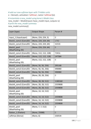
Class activation mapping (CAM) generates attention maps by weighting the feature
maps obtained from the last convolutional layer in a network. A gradient- weighted
class activation mapping (Grad-CAM) is another common method, which generates
an attention map by using gradient values calculated at backpropagation process.
This method is widely used for a general analysis of CNNs because it can be applied
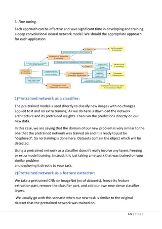
to any networks. Fig. 10 shows example attention maps of CAM and Grad-CAM.
Figure3-11 attention maps of CAM and Grad-CAM. (cite from reference [22]).
Visual explanation methods have been developed for general image recognition
tasks while visual explanation for autonomous driving has been also proposed.
Visual backprop is developed for visualize the intermediate values in a CNN, which
accumulates feature maps for each convolutional layer to a single map.

67. 66 | P a g e
This enables us to understand where the network highly responds to the input
image. Reference proposes a Regression-type Attention Branch Network in which
a CNN is divided into a feature extractor and a regression branch, as shown in
Fig3-12, with an attention branch inserted that outputs an attention map that
serves as a visual explanation. By providing vehicle speed in fully connected layers
and through end-to-end learning of each branch of Regression-type Attention
Branch Network, control values for steering and throttle for various scenes can be
output, and also output the attention map that describes the location in which the
control value was output on the input image.
Fig3-13 shows an example of visualization of attention map during Regression-type
Attention Branch Network-based autonomous driving. S and T in the figure is the
steering value and throttle value, respectively. Fig3-13 (a) shows a scene where the
road curves to the right where there is a strong response to the center line of the
road, and the steering output value is a positive value indicating the right direction.
On the other hand, Fig3-13 (b) is a scene where the road curves to the left, the
steering output value is a negative value indicating the left direction, and the
attention map responds strongly to the white line on the right. By visualizing the
attention map in this way, it can be said that the center line of the road and the
position of the lane are observed for estimation of the steering value. Also, in the
scene where the car stops as shown in Fig3-13 (c), the attention map strongly
responds to the brake lamp of the vehicle ahead. The throttle output is 0, which
indicates that the accelerator and the brake are not pressed. Therefore, it is
understood that the condition of the vehicle ahead is closely watched in the
determination of the throttle. In addition, the night travel scenario in Fig3-13 (d)
shows a scene of following a car ahead, and it can be seen that the attention map
strongly responds to the car ahead because the road shape ahead is unknown. It is
possible to visually explain the judgment grounds through output of attention map
in this way.

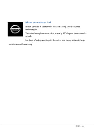
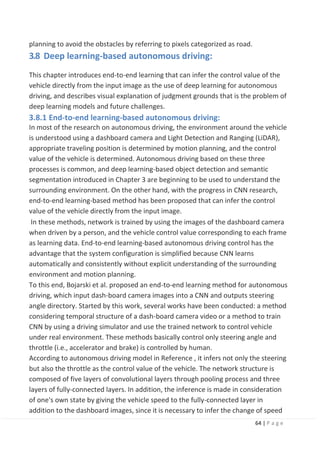
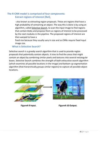
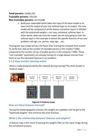
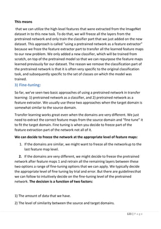
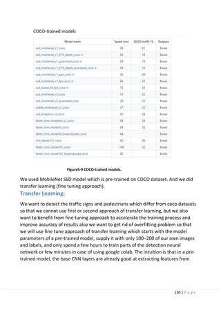
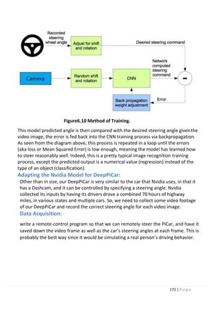
68. 67 | P a g e
Figure3-12 Regression-type Attention Branch Network. (cite from reference [17].
Figure3-13 Attention map-based visual explanation for self-driving.
3.8.3 Future challenges:
The visual explanations enable us to analyze and understand the internal state of
deep neural networks, which is efficient for engineers and researchers. One of the
future challenges is explanation for end users, i.e., passengers on a self-driving
vehicle. In case of fully autonomous driving, for instance, when lanes are suddenly
changed even when there are no vehicles ahead or on the side, the passenger in the
car may be concerned as to why the lanes were changed. In such cases, the
attention map visualization technology introduced in Section 4.2 enables people to
understand the reason for changing lanes. However, visualizing the attention map in
a fully automated vehicle does not make sense unless a person on the autonomous
vehicle always sees it. A person in an autonomous car, that is, a person whoreceives
the full benefit of AI, needs to be informed of the judgment grounds in the form of
text or voice stating, “Changing to left lane as a vehicle from the rear is approaching

69. 68 | P a g e
with speed.” Transitioning from recognition results and visual explanation to verbal
explanation will be the challenges to confront in the future. In spite of the fact that
several attempts have been conducted for this purpose, it does not still achieve
sufficient accuracy and flexible verbal explanations.
Also, in the more distant future, such verbal explanation functions will eventually
not be used. At first, people who receive the full benefit of autonomous driving find
it difficult to accept, but a sense of trust will be gradually created by repeating the
verbal explanations. Thus, if confidence is established between autonomous driving
AI and the person, the verbal explanation functions will not be required, and it can
be expected that AI-based autonomous driving will be widely and generally
accepted.
3.9 Conclusion:
This explains how deep learning is applied in image recognition tasks and introduces
the latest image recognition technology using deep learning. Image recognition
technology using deep learning is the problem of finding an appropriate mapping
function from a large amount of data and teacher labels. Further, it is possible to
solve several problems simultaneously by using multitask learning.
Future prospects not only include “recognition” for input images, but also high
expectations for the development of end-to-end learning and deep reinforcement
learning technologies for “judgment” and “control” of autonomous vehicles.
Moreover, citing judgment grounds for output of deep learning and deep
reinforcement learning is a major challenge in practical application, and it is
desirable to expand from visual explanation to verbal explanation through
integration with natural language processing.

70. 69 | P a g e
Object Detection
Chapter 3

71. 70 | P a g e
4.1 Introduction:
Object detection is a computer vision task that involves both main tasks:
1) Localizing one or more objects within an image, and
2) Classifying each object in the image
This is done by drawing a bounding box around the identified object with its
predicted class. This means that the system doesn’t just predict the class of the
image like in image classification tasks. It also predicts the coordinates of the
bounding box that fits the detected object.
It is a challenging computer vision task because it requires both successful object
localization in order to locate and draw a bounding box around each object in an
image, and object classification to predict the correct class of object that was
localized.
Image Classification vs. Object Detection tasks.

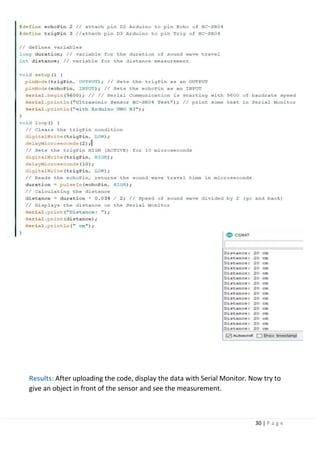
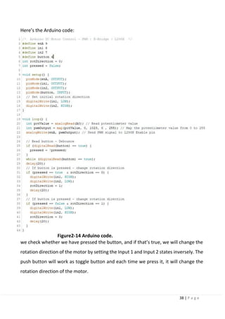
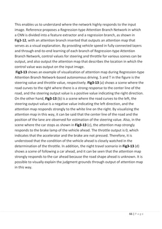
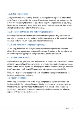
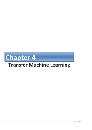
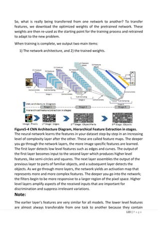
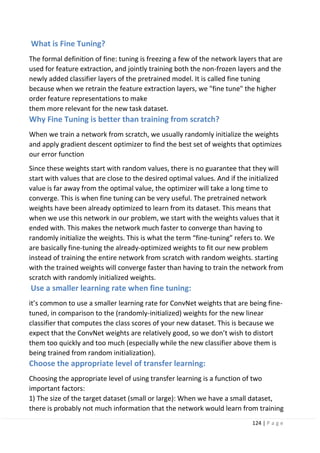
72. 71 | P a g e
Figure4-1 Classification and Object Detection.
Object detection is widely used in many fields. For example, in self-driving
technology, we need to plan routes by identifying the locations of vehicles,
pedestrians, roads, and obstacles in the captured video image. Robots often
perform this type of task to detect targets of interest. Systems in the security field
need to detect abnormal targets, such as intruders or bombs.
Now that you understand what object detection is and what differentiates it from
image classification tasks, let’s take a look at the general framework of object
detection projects.
1. First, we will explore the general framework of the object detection algorithms.
2. Then, we will dive deep into three of the most popular detection algorithms:
a. R-CNN family of networks
b. SSD
c. YOLO family of networks [3]
4.2 General object detection framework:
Typically, there are four components of an object detection framework.

73. 72 | P a g e
4.2.1 Region proposal:
An algorithm or a deep learning model is used to generate regions of interest ROI
to be further processed by the system. These region proposals are regions that the
network believes might contain an object and output a large number of bounding
boxes with an objectness score. Boxes with large objectness score are then passed
along the network layers for further processing.
4.2.2 Feature extraction and network predictions:
visual features are extracted for each of the bounding boxes, they are evaluated
and it is determined whether and which objects are present in the proposals based
on visual features (i.e. an object classification component).
4.2.3 Non-maximum suppression (NMS):
At this step, the model has likely found multiple bounding boxes for the same
object. Non-max suppression helps avoid repeated detection of the same instance
by combining overlapping into a single bounding box for each object.
4.2.4 Evaluation metrics:
similar to accuracy, precision, and recall metrics in image classification tasks object
detection systems have their own metrics to evaluate their detection performance.
In this section we will explain the most popular metrics like mean average precision
(mAP), precision-recall curve (PR curve), and intersection over union (IoU).
Now, let’s dive one level deeper into each one of these components to build an
intuition on what their goals are.
4.3 Region proposals:
In this step, the system looks at the image and proposes regions of interest for
further analysis. The regions of interest (ROI) are regions that the systembelieves
that they have a high likelihood that they contain an object, called objectness
score. Regions with high objectness score are passed to the next steps whereas,
regions with low score are abandoned

74. 73 | P a g e
Figure4-2 Low and Hight objectness score.
4.3.1 approaches to generate region proposals:
Originally, the ‘selective search’ algorithm was used to generate object proposals.
Other approaches use more complex visual features extracted by a deep neural
network from the image to generate regions (for example, based on the features
from a deep learning model). This step produces a lot (thousands) of bounding
boxes to be further analyzed and classified by the network. If the objectness score
is above a certain threshold, then this region is considered a foreground and
pushed forward in the network Note that this threshold is configurable based on
your problem. If the threshold is too low, your network will exhaustively generate
all possible proposals and you will have better chances to detect all objects in the
image.
On the flip side, this will be very computationally expensive and will slow down
your detections. So there is a trade-off that is made with region proposal
generation is the number of regions vs. the computational complexity and the right
approach is to use problem-specific information to reduce the number of ROI’s.

75. 74 | P a g e
Figure4.3 An example of selective search applied to an image. A threshold can be tuned in the SS
algorithm to generate more or fewer proposals.
Network predictions:
This component includes the pretrained CNN network that is used for feature
extraction to extract features from the input image that are representative for the
task at hand and use these features to determine the class of the image.
In object detection frameworks, people typically use pretrained image classification
models to extract visual features, as these tend to generalize fairly well. For
example, a model trained on the MS COCO or ImageNet dataset is able to extract
fairly generic features.
In this step, the network analyzes all the regions that have been identified with high
likelihood of containing an object and makes two predictions for each region:
Bounding box prediction:
the coordinates that locate the box surrounding the object. The bounding box
coordinates are represented as the following tuple (x, y, w, h). Where the x and y
are the coordinates of the center point of the bounding box and w and h are the
width and height of the box.

76. 75 | P a g e
Class prediction:
this is the classic softmax function that predicts the class probability
for each object.
Since there are thousands of regions proposed, each object will always have
multiple bounding boxes surrounding it with the correct classification.
We just need one bounding box for each object for most problems. Because what if
we are building a system to count dogs in an image? Our current system will count
5 dogs. We don’t want that. This is when the nonmaximum suppression technique
comes in handy. Object detector predicting 5 bounding boxes for the dog in the
image.
Figure4.4 Class prediction.
4.3.2 Non-maximum suppression (NMS):
One of the problems of object detection algorithms is that it may find multiple
detections of the same object. So, instead of creating only one bounding box
around the object, it draws multiple boxes for the same object. Non-maximum
suppression (NMS) is a technique that is used to make sure that the detection
algorithm detects each object only once. As the name implies, NMS techniquelooks
at all the boxes surrounding an object to find the box that has the maximum
prediction probabilities and suppress or eliminate the other boxes, hence the
name, non-maximum suppression.

77. 76 | P a g e
Figure4-5 Predictions before and after NMS.
4.4 Steps of how the NMS algorithm works:
1) Discard all bounding boxes that have predictions that are less than a certain
threshold, called confidence threshold. This threshold is tunable. Thismeans
that the box will be suppressed if the prediction probability is less than the
set threshold.
2) Look at all the remaining boxes and select the bounding box with thehighest
probability.
3) Then calculate the overlap of the remaining boxes that have the same class
prediction. Bounding boxes that have high overlap with each other and are
predicting the same class are averaged together. This overlap metric iscalled
Intersection Over Union (IOU).
4) The algorithm then suppresses any box that has an IOU value that is smaller
than a certain threshold (called NMS threshold). Usually the NMS thresholdis
equal to 0.5 but it is tunable as well if you want to output less or more
bounding boxes.
NMS techniques are typically standard across the different detection frameworks.
4.4.1 Object detector evaluation metrics:
When evaluating the performance of an object detector
, we use two main evaluation metrics:
(frame-per-second) FPS TO MEASURE THE DETECTION SPEED:
The most common metric that is used to measure the detection speed is the
number of frames per second (FPS). For example, Faster R-CNN operates at only 7

78. 77 | P a g e
(FPS) whereas SSD operates at 59 FPS.
MEAN AVERAGE PRECISION (MAP):
The most common evaluation metric that is used in object recognition tasks is
‘mAP’, which stands for mean average precision. It is a percentage from 0 to 100
and higher values are typically better, but its value is different from the accuracy
metric in classification. To understand the mAP, we need to understand the
Intersection Over Union (IOU) and the Precision-Recall Curve (PR Curve)
4.4.1.3 Intersection Over Union (IOU):
It is a measure that evaluates the overlap between two bounding boxes: the
ground truth bounding box Bground truth (box that we feed network to train on)
and the predicted bounding box Bpredicted (output of network).
By applying the IOU, we can tell if a detection is valid (True Positive) or not (False
Positive).
Figure4-6 Intersection Over Union (EQU)
Figure4-7 Ground-truth and
predicted box.

79. 78 | P a g e
intersection over the union value ranges from 0, meaning no overlap at all, to 1
which means that the two bounding boxes 100% overlap on each other. The higher
the overlap between the two bounding boxes (IOU value), the better.
To calculate the IoU of a prediction, we need:
The ground-truth bounding box (Bground truth) the hand-labeled bounding box
that is created during the labeling process. The predicted bounding box
(Bpredicted) from our model.
IoU is used to define a “correct prediction”. Meaning, a “correct” prediction (True
Positive) is
one that has IoU greater than some threshold. This threshold is a tunable value
depending on the challenge but 0.5 is a standard value. For example, some
challenges like MS COCO, uses mAP@0.5 meaning IOU threshold = 0.5 or
mAP@0.75 meaning IOU threshold = 0.75. This means that if the IoU is above this
threshold is considered a True Positive (TP) and if it is below it is considered as a
False Positive (FP).
4.5 Precision-Recall Curve (PR Curve):
Precision:
is a metric that quantifies the number of correct positive predictions made. It is
calculated as the number of true positives divided by the total number of true
positives and false positives.
Precision = TruePositives / (TruePositives + FalsePositives)
Recall:
is a metric that quantifies the number of correct positive predictions made out of
all positive predictions that could have been made. It is calculated as the number of
true positives divided by the total number of true positives and false negatives (e.g.
it is the true positive rate).
Recall = TruePositives / (TruePositives + FalseNegatives)
The result is a value between 0.0 for no recall and 1.0 for full or perfect recall. Both
the precision and the recall are focused on the positive class (the minority class)
and are unconcerned with the true negatives (majority class).
PR Curve:
Plot of Recall (x) vs Precision (y). A model with perfect skill is depicted as a point at
a coordinate of (1,1). A skillful model is represented by a curve that bows towards a

80. 79 | P a g e
coordinate of (1,1). A no-skill classifier will be a horizontal line on the plot with a
precision that is proportional to the number of positive examples in thedataset.
For a balanced dataset this will be 0.5.
Figure4-8 PR Curve.
A detector is considered good if its precision stays high as recall increases, which
means that if you vary the confidence threshold, the precision and recall will still be
high. On the other hand, a poor detector needs to increase the number of FPs
(lower precision) in order to achieve a high recall. That's why the PR curve usually
starts with high precision values, decreasing as recall increases.
Now, that we have the PR curve, we calculate the AP (Average Precision) by
calculating the Area Under the Curve (AUC). Then finally, mAP for object detection
is the average of the AP calculated for all the classes. It is also important to note
that for some papers, they use AP and mAP interchangeably.
4.6 Conclusion:
To recap, the mAP is calculated as follows:
1. Each bounding box will have an objectness score associated (probabilityof
the box containing an object).
2. Precision and recall are calculated.
3. Precision-recall curve (PR curve) is computed for each class by varying the
score threshold.
4. Calculate the average precision (AP): it is the area under the PR curve. Inthis
step, the AP is computed for each class.
5. Calculate mAP: the average AP over all the different classes.
Most deep learning object detection implementations handle computing mAP
for you.

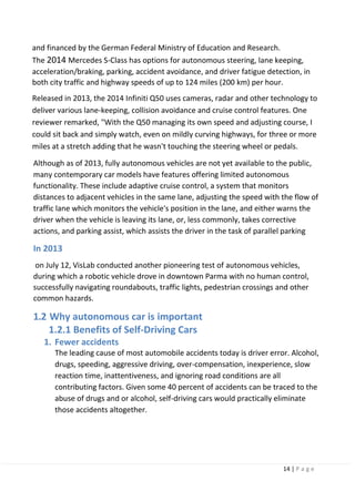
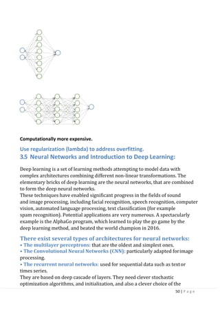
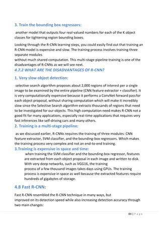
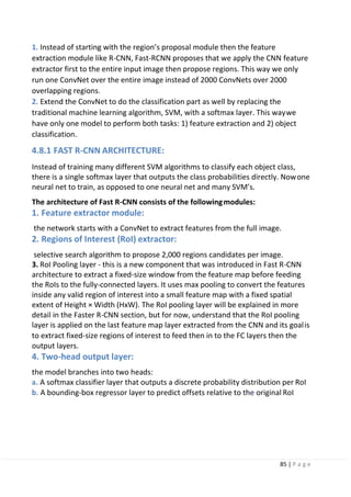
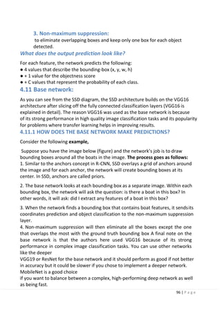
81. 80 | P a g e
Now, that we understand the general framework of object detection algorithms,
let’s dive deeper into three of the most popular detection algorithms.
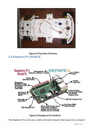
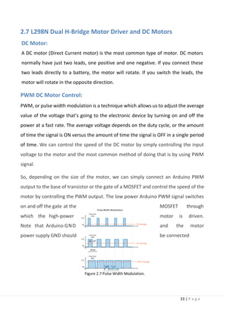
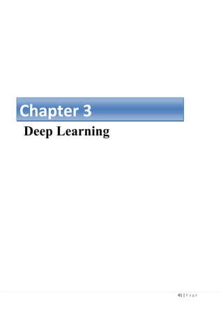
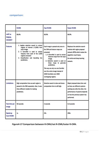
4.7 Region-Based Convolutional Neural Networks (R-CNNs) [high mAP
and low FPS]:
Developed by Ross Girshick et al. in 2014 in their paper “Rich feature hierarchies for
accurate object detection and semantic
segmentation”.
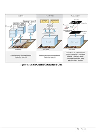
The R-CNN family has then expanded to include Fast-RCNN and Faster-RCNN that
came out in 2015 and 2016.
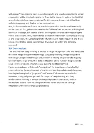
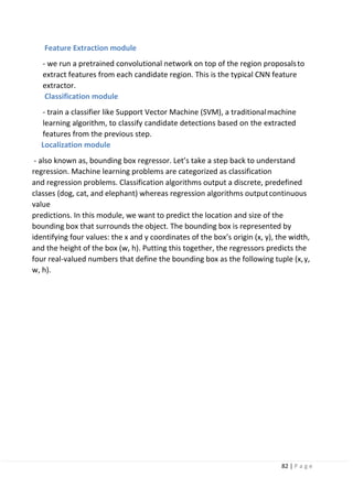
R-CNN:
The R-CNN is the least sophisticated region-based architecture in its family, but itis
the basis for understanding how multiple object recognition algorithms work for all
of them. It may have
been one of the first large and successful applications of convolutional neural
networks to the problem of object detection and localization that paved the way
for the other advanced detection algorithms.
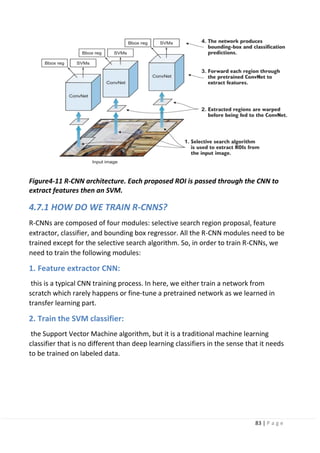
Figure4-9 Regions with CNN features.

82. 81 | P a g e
The R-CNN model is comprised of four components:
Extract regions of interest (RoI):
- also known as extracting region proposals. These are regions that have a
high probability of containing an object. The way this is done is by using an
algorithm, called Selective Search, to scan the input image to find regions
that contain blobs and propose them as regions of interest to be processed
by the next modules in the pipeline. The proposed regions of interest are
then warped to have a
fixed size because they usually vary in size and as CNNs require fixed input
image size.
What is Selective Search?
Selective search is a greedy search algorithm that is used to provide region
proposals that potentially contain objects. It tries to find the areas that might
contain an object by combining similar pixels and textures into several rectangular
boxes. Selective Search combines the strength of both exhaustive search algorithm
(which examines all possible locations in the image) and bottom-up segmentation
algorithm (that hierarchically groups similar regions) to capture all possible object
locations.
Figure4-9 Input. Figure4-10 Output.

83. 82 | P a g e
Feature Extraction module
- we run a pretrained convolutional network on top of the region proposalsto
extract features from each candidate region. This is the typical CNN feature
extractor.
Classification module
- train a classifier like Support Vector Machine (SVM), a traditionalmachine
learning algorithm, to classify candidate detections based on the extracted
features from the previous step.
Localization module
- also known as, bounding box regressor. Let’s take a step back to understand
regression. Machine learning problems are categorized as classification
and regression problems. Classification algorithms output a discrete, predefined
classes (dog, cat, and elephant) whereas regression algorithms outputcontinuous
value
predictions. In this module, we want to predict the location and size of the
bounding box that surrounds the object. The bounding box is represented by
identifying four values: the x and y coordinates of the box’s origin (x, y), the width,
and the height of the box (w, h). Putting this together, the regressors predicts the
four real-valued numbers that define the bounding box as the following tuple (x,y,
w, h).

84. 83 | P a g e
Figure4-11 R-CNN architecture. Each proposed ROI is passed through the CNN to
extract features then an SVM.
4.7.1 HOW DO WE TRAIN R-CNNS?
R-CNNs are composed of four modules: selective search region proposal, feature
extractor, classifier, and bounding box regressor. All the R-CNN modules need to be
trained except for the selective search algorithm. So, in order to train R-CNNs, we
need to train the following modules:
1. Feature extractor CNN:
this is a typical CNN training process. In here, we either train a network from
scratch which rarely happens or fine-tune a pretrained network as we learned in
transfer learning part.
2. Train the SVM classifier:
the Support Vector Machine algorithm, but it is a traditional machine learning
classifier that is no different than deep learning classifiers in the sense that it needs
to be trained on labeled data.

85. 84 | P a g e
3. Train the bounding box regressors:
another model that outputs four real-valued numbers for each of the K object
classes for tightening region bounding boxes.
Looking through the R-CNN learning steps, you could easily find out that training an
R-CNN model is expensive and slow. The training process involves training three
separate modules
without much shared computation. This multi-stage pipeline training is one of the
disadvantages of R-CNNs as we will see next.
4.7.2 WHAT ARE THE DISADVANTAGES OF R-CNN?
1. Very slow object detection:
selective search algorithm proposes about 2,000 regions of interest per a single
image to be examined by the entire pipeline (CNN feature extractor + classifier). It
is very computationally expensive because it performs a ConvNet forward passfor
each object proposal, without sharing computation which will make it incredibly
slow since the Selective Search algorithm extracts thousands of regions that need
to be investigated for our objects. This high computation need makes R-CNN not a
good fit for many applications, especially real-time applications that requires very
fast inferences like self-driving cars and many others.
2. Training is a multi-stage pipeline:
as we discussed earlier, R-CNNs requires the training of three modules: CNN
feature extractor, SVM classifier, and the bounding-box regressors. Which makes
the training process very complex and not an end-to-end training.
3.Training is expensive in space and time:
when training the SVM classifier and the bounding-box regressor, features
are extracted from each object proposal in each image and written to disk.
With very deep networks, such as VGG16, the training
process of a few thousand images takes days using GPUs. The training
process is expensive in space as well because the extracted features require
hundreds of gigabytes of storage.
4.8 Fast R-CNN:
Fast R-CNN resembled the R-CNN technique in many ways, but
improved on its detection speed while also increasing detection accuracy through
two main changes:

86. 85 | P a g e
1. Instead of starting with the region’s proposal module then the feature
extraction module like R-CNN, Fast-RCNN proposes that we apply the CNN feature
extractor first to the entire input image then propose regions. This way we only
run one ConvNet over the entire image instead of 2000 ConvNets over 2000
overlapping regions.
2. Extend the ConvNet to do the classification part as well by replacing the
traditional machine learning algorithm, SVM, with a softmax layer. This waywe
have only one model to perform both tasks: 1) feature extraction and 2) object
classification.
4.8.1 FAST R-CNN ARCHITECTURE:
Instead of training many different SVM algorithms to classify each object class,
there is a single softmax layer that outputs the class probabilities directly. Nowone
neural net to train, as opposed to one neural net and many SVM’s.
The architecture of Fast R-CNN consists of the followingmodules:
1. Feature extractor module:
the network starts with a ConvNet to extract features from the full image.
2. Regions of Interest (RoI) extractor:
selective search algorithm to propose 2,000 regions candidates per image.
3. RoI Pooling layer - this is a new component that was introduced in Fast R-CNN
architecture to extract a fixed-size window from the feature map before feeding
the RoIs to the fully-connected layers. It uses max pooling to convert the features
inside any valid region of interest into a small feature map with a fixed spatial
extent of Height × Width (HxW). The RoI pooling layer will be explained in more
detail in the Faster R-CNN section, but for now, understand that the RoI pooling
layer is applied on the last feature map layer extracted from the CNN and its goalis
to extract fixed-size regions of interest to feed then in to the FC layers then the
output layers.
4. Two-head output layer:
the model branches into two heads:
a. A softmax classifier layer that outputs a discrete probability distribution per RoI
b. A bounding-box regressor layer to predict offsets relative to the original RoI

87. 86 | P a g e
4.8.2 DISADVANTAGES OF FAST R-CNN:
The selective search algorithm for generating region proposals is very slow and it is
generated separately by another model.
4.9 Faster R-CNN:
Similar to Fast R-CNN, the image is provided as an input to a convolutional network
which provides a convolutional feature map. Instead of using a selective search
algorithm on the feature map to identify the region proposals, a network is used to
predict the region proposals as part of the training process, called Region Proposal
Network (RPN). The predicted region proposals are then reshaped using a Rpooling
layer then used to classify the image within the proposed region and predict the
offset values for the bounding boxes. These improvements both reduce the
number of region proposals and accelerate the
test-time operation of the model to near real-time with then state-of-the-art
performance.
4.9.1 FASTER R-CNN ARCHITECTURE:
The architecture of Faster R-CNN can be described by two main networks:
1. Region Proposal Network (RPN)
selective search is replaced by a ConvNet that to propose regions of interest (RoI)
from the last feature maps of the feature extractor to be considered for
investigations. RPN has two outputs; the “objectness score” (object or no object)
and the box location

88. 87 | P a g e
2. Fast R-CNN
consists of the typical components of Fast R-CNN:
a. Base network for Feature extractor: a typical pre-trained CNN model to extract
features from the input image.
b. ROI pooling layer: to extract fixed-size regions of interest.
c. Output layer: contains 2 fully-connected layers:
1) a softmax classifier to output the class probability, and
2) a bounding-box regression CNN to the bounding box predictions.
Figure4.12 Fast R-CNN.
Faster R-CNN architecture has two main components:
1) a region proposal network (RPN), which Faster R-CNN architecture has two main
components:
a.a region proposal network (RPN):
which identifies regions that may contain objects of interest andtheir
approximate location
b.a Fast R-CNN network:
which classifies objects, and refines their location, defined using bounding boxes.

89. 88 | P a g e
The two components share the convolutional layers of the pre-trained VGG-16As
you can see in the Faster R-CNN architecture diagram (Figure), the input image is
presented to the network and its features are extracted via a pre-trained CNN.
These features, in parallel, are sent to two different components of the Faster R-
CNN architecture:
1. The RPN to determine where in an image a potential object could be. At this point
we do not know what the object is, just that there is potentially an object at a
certain location in the image.
1. ROI pooling to extract fixed-size windows of features This architectureachieves
an end-to-end trainable and the complete object detection pipeline where all
the required components take place inside the network, including:
2. Base network feature extractor
3. Regions proposal
4. ROI pooling
5. Object classification
6. Bounding box regressor
BASE NETWORK TO EXTRACT FEATURES:
Similar to Fast R-CNN, the first step is using a pretrained CNN and slice off its
classification part. The base network is used to extract features from the input
image. In this component, you can use any of the popular CNN architectures based
onthe problem that you are trying to solve.
For example, MobileNet, a smaller and efficient network architecture optimizedfor
speed, has approximately 3.3M parameters, while ResNet-152 (152 layers), once
the state of the art in the ImageNet classification competition, has around 60M.
Most recently, new architectures like DenseNet are both improving results while
lowering the number of parameters.
REGION PROPOSAL NETWORK (RPN):
The region proposal network identifies regions that could potentially contain
objects of interest, based on the last feature map of the pre-trained convolutional
neural network. RPN is also known as the ‘attention network’ because it guides the
networks attention to interesting regions in the image. Faster R-CNN uses Region
Proposal Network (RPN) to bake the region
proposal directly into the R-CNN architecture instead of running a Selective Search
algorithm to extract regions of interests.

90. 89 | P a g e
Figure4-14 The RPN classifier predicts the objectness score which is the probability
of an image containing an object (foreground) or a background.
Fully-convolutional networks (FCN):
One important aspect of object detection networks is that they should be fully
convolutional. A fully convolutional neural network means that the network does
not contain any fully-connected (FC) layers typically found at the end of anetwork
prior to making output predictions.
In the context of image classification, removing the fully-connected layersis
normally accomplished by applying
average pooling across the entire volume prior to a single dense softmax classifier
used to output the final predictions.
A fully-convolutional network (FCN) has two main benefits:
1. Faster because it contains only convolution operations and no FC layers.
2. Able to accept images of any spatial resolution (width and height), providedthat
the image and network can fit into
memory, of course.
Note:
Being an FCN makes the network invariant to the size of the input image. However,
in practice, we might want to stick to a constant input size due to various problems
that only show their heads when we are implementing the algorithm. A big one
amongst these problems is that if we want to process our images in batches(images
in batches can be processed in parallel by the GPU, leading to speed boosts), we
need to have all images of fixed height and width.

91. 90 | P a g e
HOW DOES THE REGRESSOR PREDICT THE BOUNDING BOX?
To answer this question, let’s first define the bounding box. It is the box that
surrounds the object and is identified by the following tuple (x, y, w, h). Where the
x and y are the coordinates in the image that describes the center of the bounding
box and the h and w are the height and width of the bounding box. Researchers
found that defining the (x, y) coordinates of the center point could be challenging
because we have to enforce some rules to make sure that the network predicts
values inside the boundaries of the image. Instead, we can create reference boxes
called anchor boxes in the image and make the regression layer predict the offsets
from these boxes called deltas (Δx, Δy, Δw, Δh) to adjust the anchor boxes to better
fit the object to get the final proposals.
Figure 4-15 Anchor boxes at the center of each sliding window.IoU is calculated to
select the bounding box the overlaps the most with the ground-truth.
Anchor boxes:
using a sliding window approach, RPN generates k regions for each location in the
feature map. These regions, are represented as boxes called anchor boxes. The
anchors are all centered in the middle of their corresponding sliding window, and
differ in terms of scale and aspect ratio to cover a wide variety of objects. These are
fixed bounding boxes that are placed throughout the image to be used for
reference when first predicting object locations. In their paper, Ross Girshick ET. Al
generated 9 anchor boxes all have the same center but with 3 different aspect
ratios and 3 different scales as shown below.

92. 91 | P a g e
HOW DO WE TRAIN THE RPN?
RPN is trained using human annotators to label the bounding boxes, this labeled
box is called the ground-truth. For each anchor box, the overlap probability value
(p) is computed which indicates how much these anchors overlap with the ground-
truth bounding boxes.
If an anchor has high overlap with a ground-truth bounding box, then it is likely that
the anchor box includes an object of interest, and it is labeled as positive with
respect to the object versus no object classification task.
Nowadays, ResNet architectures have mostly replaced VGG as a base network for
extracting features. The obvious advantage of ResNet over VGG is that it has much
more layers (deeper) giving it more capacity to learn very complex features. This is
true for the classification task and should be equally true in the case of object
detection. Also, ResNet makes it easy to train deep models with the use of residual
connections and batch normalization, which was not invented when VGG was first
released.

93. 92 | P a g e
Figure4-16 R-CNN,Fast R-CNN,Faster R-CNN.

94. 93 | P a g e
comparison:
Figure4-17 Comparison between R-CNN,Fast R-CNN,Faster R-CNN.

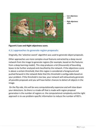
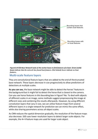
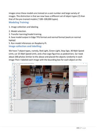
95. 94 | P a g e
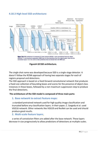
4.10 Single Shot Detection (SSD) [Detection Algorithm UsedIn
Our Project]:
The paper about SSD: Single Shot MultiBox Detector was released in November
2016 by C. Szegedy et al. Single Shot Detection network reached new records in
terms of performance and precision for object detection tasks, scoring over 74%
mAP (mean Average Precision) at 59 frames per second (FPS) on standard datasets
such as PascalVOC and MS COCO.
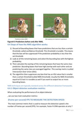
4.10.1 Very important note:
The most common metric that is used to measure the detection speed isthe
number of frames per second (FPS). For example,
Faster R-CNN operates at only 7 frames per second (FPS). There have been many
attempts to build faster detectors by attacking each stage of the detection pipeline
but so far, significantly increased speed comes only at the cost of significantly
decreased detection accuracy. In this section you will see why single-stage
networks like SSD can achieve faster detections that are more suitable for real-time
detections.
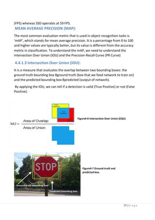
For benchmarking, SSD300 achieves 74.3% mAP at 59 FPS while SSD512 achieves
76.8% mAP at 22 FPS, which outperforms Faster R-CNN (73.2% mAP at 7 FPS).
SSD300 refers to the size of the input image of 300x300 and SSD512 refers to an
input image of size = 512x512.
4.10.2 SSD IS A SINGLE-STAGE DETECTOR:
The R-CNN family is a multi-stage detector. Where the network first predict the
objectness score of the bounding box then pass this box through a classifier to
predict the class probability.
In single-stage detectors like SSD and YOLO (explained later), the convolutional
layers make both predictions directly in one shot, hence the name Single Shot
Detector. Where the image is passed once through the network and the objectness
score for each bounding box is predicted using logistic regression to indicate the
level of overlap with the ground truth. If the bounding box overlaps 100% with the
ground truth, the objectness score is = 1 and if there is no overlap, the objectness
score = 0. We then set a threshold value (0.5) that says: “if the objectness score is
above 50%, then this bounding box likely has an object of interest and we get
predictions, if it is less than 50%, we ignore the prediction.”

96. 95 | P a g e
4.10.3 High level SSD architecture:
Figure4-18 SSD architecture.
The single shot name was developed because SSD is a single-stage detector. It
doesn’t follow the RCNN approach of having two separate stages for each of
regions proposal and detections.
The SSD approach is based on a feed-forward convolutional network that produces
a fixed-size collection of bounding boxes and scores for the presence of object class
instances in those boxes, followed by a non-maximum suppression step to produce
the final detections.
The architecture of the SSD model is composed of three main parts:
1. Base network to extract feature maps:
a standard pretrained network used for high quality image classification and
truncated before any classification layers. In their paper, C. Szegedy et al. used
VGG16 network. Other networks like VGG19 and ResNet can be used and should
produce good results.
2. Multi-scale feature layers:
a series of convolution filters are added after the base network. These layers
decrease in size progressively to allow predictions of detections at multiple scales.

97. 96 | P a g e
3. Non-maximum suppression:
to eliminate overlapping boxes and keep only one box for each object
detected.
What does the output prediction look like?
For each feature, the network predicts the following:
● 4 values that describe the bounding-box (x, y, w, h)
● + 1 value for the objectness score
● + C values that represent the probability of each class.
4.11 Base network:
As you can see from the SSD diagram, the SSD architecture builds on the VGG16
architecture after slicing off the fully connected classification layers (VGG16 is
explained in detail). The reason VGG16 was used as the base network is because
of its strong performance in high quality image classification tasks and its popularity
for problems where transfer learning helps in improving results.
4.11.1 HOW DOES THE BASE NETWORK MAKE PREDICTIONS?
Consider the following example,
Suppose you have the image below (figure) and the network’s job is to draw
bounding boxes around all the boats in the image. The process goes as follows:
1. Similar to the anchors concept in R-CNN, SSD overlays a grid of anchors around
the image and for each anchor, the network will create bounding boxes at its
center. In SSD, anchors are called priors.
2. The base network looks at each bounding box as a separate image. Within each
bounding box, the network will ask the question: is there a boat in this box? In
other words, it will ask: did I extract any features of a boat in this box?
3. When the network finds a bounding box that contains boat features, it sendsits
coordinates prediction and object classification to the non-maximum suppression
layer.
4. Non-maximum suppression will then eliminate all the boxes except the one
that overlaps the most with the ground truth bounding box A final note on the
base network is that the authors here used VGG16 because of its strong
performance in complex image classification tasks. You can use other networks
like the deeper
VGG19 or ResNet for the base network and it should perform as good if not better
in accuracy but it could be slower if you chose to implement a deeper network.
MobileNet is a good choice
if you want to balance between a complex, high-performing deep network as well
as being fast.

98. 97 | P a g e
Figure4.19 SSD Base Network looks at the anchor boxes to find features of a boat. Green (solid)
boxes indicate that the network has found boat features. Red (dotted) boxes indicate no boat
features.
Multi-scale feature layers
They are convolutional feature layers that are added to the end of thetruncated
base network. These layers decrease in size progressively to allow predictions of
detections at multiple scales.
As you can see, the base network might be able to detect the horses’ featuresin
the background but it might fail to detect the horse that is closest to the camera.
Can you see horse features in this bounding box in Figure? No. To deal with objects
of different scales in an image, some methods suggest preprocessing the image at
different sizes and combining the results afterwards. However, by using different
convolution layers that vary in size, we can utilize feature maps from several
different layers in a single network for prediction we can mimic the same effect,
while also sharing parameters across all object scales.
As CNN reduces the spatial dimension gradually, the resolution of the feature maps
also decrease. SSD uses lower resolution layers to detect larger scale objects. For
example, the 4× 4 feature maps are used for larger scale object.

99. 98 | P a g e
Figure4-20 Right image - lower resolution feature maps detect larger scale objects. Left image –
higher resolution feature maps detect smaller scale objects.
The multi-scale feature layers resize the image dimensions and keep the bounding
boxes sizes so that they can fit the larger horse. In reality, convolutional layers do
not literally reduce the size of the image. This is just for illustration to help us to
intuitively understand the concept. In reality it is not just resized, it actually goes
through the convolutional process so the image won’t look anything like itself
anymore. It will be a completely random looking image but it will preserve its
features. Using a multi-scale feature maps improves the network accuracy
significantly. the table below shows a decrease in accuracy with less layers. Here is
the accuracy with different number of feature map layers used for object detection.

100. 99 | P a g e
Figure4-21 the accuracy with different number of feature map layers.
4.12.1 ARCHITECTURE OF THE MULTI-SCALE LAYERS:
The authors decided to add 6 convolutional layers that are decreasing in size. This
has been done by a lot of tuning and trial and error until they produced the best
results.
Figure4-22 Architecture of the multi-scale layers.
4.12.2 Non-maximum Suppression:
Given the large number of boxes generated by the detection layer per class during
a forward pass of SSD at inference time, it is essential to prune most of the
bounding box by applying the non-maximum suppression technique Where boxes
with a confidence loss and IoU less than a certain threshold are discarded, and only
the top N predictions are kept. This ensures only the most likely predictions are
retained by the network, while the noisier ones are removed.
SSD sorts the predictions by the confidence scores. Start from the top confidence
prediction, SSD evaluates whether any previously predicted boundary boxes have
an iou higher than 0.45 with the current prediction for the same class (the
threshold value of 0.45 is set by the authors of the original paper).

101. 100 | P a g e
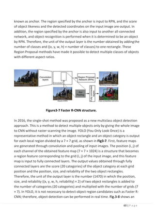
4.12.3 (YOLO) [high speed but low mAP]:
The YOLO family of models is a series of end-to-end deep learning models designed
for fast object detection, developed by joseph redmon, et al. And is considered one
of the first attempts to build a fast real-time object detector. It is one of the faster
object detection algorithms out there. Though it is no longer the most accurate
object detection algorithm, it is a very good choice when you need real-time
detection, without loss of too much accuracy.
The creators of YOLO took a different approach than the previous networks. YOLO
does not undergo the region proposal step like R-CNNs. Instead, it only predicts
over a limited number of bounding boxes by splitting the input into a grid of cells
and each cell directly predicts a bounding box and object classification. The result is
a large number of candidates bounding boxes that are consolidated into a final
prediction using non-maximum suppression.
4.13.1 Yolo versions:

102. 101 | P a g e
Figure4-23 YOLO splits the image into grids, predicts objects for each grid, then use NMS to
finalize predictions.
Although the accuracy of the models is close but not as good as Region-Based
Convolutional Neural Networks (R-CNNs), they are popular for object detection
because of their detection speed, often demonstrated in real-time on video or
camera feed input.
• YOLOv1:
YOLO Unified, Real-Time Object Detection. It is called unified because it is asingle
detection network that unifies the two components of a detector; object detector
and class predictor.
• YOLOv2:
YOLO9000 - Better, Faster, Stronger that is capable of detecting over 9,000 objects,
hence the name YOLO9000. It has been trained on ImageNet and MS COCO
datasets and has achieved 16% mean Average Precision (mAP) which is not quite
good but it was very fast during test time.
• YOLOv3:
An Incremental Improvement. YOLOv3 is significantly larger than previous models
and has achieved mAP of 57.9% which is the best results yet out of the YOLO family
of object detectors.
4.13.2 How YOLOv3 works:
• The YOLO network splits the inputimage into a grid of S×S cells. If the center
of the ground truth box falls into a cell, that cell is responsible for detecting
the existence of that object.
• Each grid cell predicts B number of bounding boxes and theirobjectness
score along with their class predictions as follows:

103. 102 | P a g e
1. Coordinates of B bounding boxes:
similar to previous detectors, YOLO predicts 4 coordinates for each bounding
box (bx,by,bw,bh). Where x and y are set to be offset of a cell location.
2. Objectness score (P0):
indicates the probability that the cell contains an object. The objectness
score is passed through a sigmoid function to be treated as a probability with
a value range between 0 and 1. The objectness score is calculated as follows:
P0 = Pr (containing an object) x IoU (pred, truth).
3. Class prediction:
if the bounding box contains an object, the network predicts the probability
of K number of classes. Where K is the total number of classes in your
problem.
Figure4-24 YOLOv3 workflow.

104. 103 | P a g e
4.13.3 Prediction across different scale:
• YOLOv3 has 9 anchors to allow for prediction at 3 different scales per cell.
The detection layer makes detection at feature maps of three differentsizes,
having strides 32, 16, and 8 respectively. This means, with an input image of
size 416 x 416, we make detections on scales 13 x 13, 26 x 26 and 52 x 52.
The 13 x 13 layer is responsible for detecting large objects, the 26 x 26 layer
is for detecting medium objects, and the 52x52 layer detects the smaller
objects.
• This results in the prediction of 3 bounding boxes for each cell (B=3). That’s
why in Figure you see that the prediction feature map is predicting box1,
box2 , and box3. The bounding box responsible for detecting the dog willbe
the one whose anchor has the highest IoU with the ground truth box.
• Detections at different layers helps address the issue of detecting small
objects, which was a frequent complaint with YOLOv2. The up sampling
layers can help the network preserve and learn fine-grained featureswhich
are instrumental for detecting small objects.
Figure4-25 YOLOV3 Output bounding boxes.
• For an input image of size 416 x 416, YOLO predicts ((52 x 52) + (26 x 26) +13
x 13)) x 3 = 10,647 bounding boxes. That is a huge number of boxes for an
output.
• In our dog example, we have only one object. We want only one bounding
box around this object. How do we reduce the boxes down from 10,647 to1?

105. 104 | P a g e
• First, we filter boxes based on theirobjectness score. Generally, boxes having
scores below a threshold are ignored.
• Second, we use Non-maximum Suppression (NMS). NMS intends to curethe
problem of multiple detections of the same image.
• For example, all the 3 bounding boxes of the red grid cell at the center ofthe
image may detect a box or the adjacent cells may detect the sameobject.
4.13.4 YOLOv3 Architecture:
• YOLO is a single neural network that unifies object detection and
classifications into one end-to-end network. The neural networkarchitecture
was inspired by the GoogLeNet model (Inception) for feature extraction.
Instead of the inception modules used by GoogLeNet, YOLO uses 1x1
reduction layers followed by 3x3 convolutional layers. The authors calledthis
Darknet.
Figure4-26 neural network architecture.
4.13.4 Comparisons:
After exploring different techniques that used in object detection, we will discuss
the tools that we used in our project and used model.
First, we will take about Google Colab and tensorflow:
Google is quite aggressive in AI research. Over many years, Google developed AI
framework called TensorFlow and a development tool called Colaboratory. Today
TensorFlow is open-sourced and since 2017, Google made Colaboratory free for
public use. Colaboratory is now known as Google Colab or simply Colab.
Another attractive feature that Google offers to the developers is the use of GPU.
Colab supports GPU and it is totally free. The reasons for making it free for public

106. 105 | P a g e
could be to make its software a standard in the academics for teaching machine
learning and data science. It may also have a long-term perspective of building a
customer base for Google Cloud APIs which are sold per-use basis.
Irrespective of the reasons, the introduction of Colab has eased the learning and
development of machine learning applications.
So, let us get started with Colab.
4.14 What Colab Offers You?
• Write and execute code in Python.
• Document your code that supports mathematical equations.
• Create/Upload/Share notebooks.
• Import/Save notebooks from/to Google Drive.
• Import/Publish notebooks from GitHub.
• Import external datasets e.g. from Kaggle.
• Integrate PyTorch, TensorFlow, Keras, OpenCV.
• Free Cloud service with free GPU, CPU, or TPU.
Because of previous advantage it helped us a lot to train model, especially using the
GPU which minimize the training time a lot so that we can tune hyper parameter
such as the number of iteration (number of training steps) and also try more than
single model till reaching the model that satisfy requirements.
We used the following:
1. TensorFlow

107. 106 | P a g e
2. Python
3. OpenCV
Figure4-27 Python Figure4-28 Open CV
Figure4-29 TensorFlow.
4.14.1 Why TensorFlow?
1) TensorFlow is an end-to-end platform that makes it easy for you to buildand
deploy ML models.
2) It is open source and has large community to ease solving problems thatmay
face you.

108. 107 | P a g e
3) Easy model building
4)TensorFlow offers multiple levels of abstraction so you can choose the right one
for your needs. Build and train models by using the high-level Keras API, which
makes getting started with TensorFlow and machine learning easy.If you need more
flexibility, eager execution allows for immediate iteration and intuitivedebugging.
For large ML training tasks, use the Distribution Strategy API for distributed training
on different hardware configurations without changing the model definition.
5)Robust ML production anywhere.
6)TensorFlow has always provided a direct path to production. Whether it’s on
servers, edge devices, or the web, TensorFlow lets you train and deploy yourmodel
easily, no matter what language or platform you use.Use TensorFlow Extended
(TFX) if you need a full production ML pipeline. For running inference onmobile and
edge devices, use TensorFlow Lite. Train and deploy models in JavaScript
environments using TensorFlow.js.
7)Powerful experimentation for research
8)Build and train state-of-the-art models without sacrificing speed orperformance.
TensorFlow gives you the flexibility and control with features like the Keras
Functional API and Model Sub classing API for creation of complex topologies. For
easy prototyping and fast debugging, use eager execution.
9)TensorFlow also supports an ecosystem of powerful add-on libraries andmodels
to experiment with, including Ragged Tensors, TensorFlow Probability,
Tensor2Tensor and BERT.
10)OpenCV:
4.14.2 OpenCV (Open Source Computer Vision Library)
is a library of programming functions mainly aimed at real-time vision. Originally
developed by Intel, it was later supported by Willow Garage then Itseez (which was
later acquired by Intel). The library is cross-platform and free for use under
the open-source BSD license.
Applications:
OpenCV's application areas include:
• 2D and 3D feature toolkits.
• Egomotion estimation.
• Facial recognition system.

109. 108 | P a g e
• Gesture recognition.
• Human–computer interaction (HCI).
• Mobile robotics.
• Motion understanding.
• Object identification.
• Segmentation and recognition.
• Stereopsis stereo vision: depth perception from 2 cameras.
• Structure from motion (SFM).
• Motion tracking.
• Augmented reality.
To support some of the above areas,
OpenCV includes a statistical machine learning library that contains:
• Boosting.
• Decision tree learning.
• Gradient boosting trees.
• Expectation-maximization algorithm.
• k-nearest neighbor algorithm.
• Naive Bayes classifier.
• Artificial neural networks.
• Random forest.
• Support vector machine (SVM).
• Deep neural networks (DNN).
So that it helps a lot at projects uses deep learning. The used programming
language is python which is open source programming language.
Python as the best programming language for AI and ML are being applied across
various channels and industries, big corporations invest in these fields, and the
demand for experts in ML and AI grows accordingly. Jean Francois Puget, from IBM’s
machine learning department, expressed his opinion that
Python is the most popular language for AI and ML and based it on a
trend search results on indeed.com.
Why?
1) A great library ecosystem:
A great choice of libraries is one of the main reasons Python is the most popular
programming language used for AI. A library is a module or a group of modules
published by different sources like PyPi which include a pre-written piece of code

110. 109 | P a g e
that allows users to reach some functionality or perform different actions. Python
libraries provide base level items so developers don’t have to code them from the
very beginning every time. ML requires continuous data processing, and Python’s
libraries let you access, handle and transform data. These are some of the most
widespread libraries you can use for ML and AI:
• Scikit-learn:
for handling basic ML algorithms like clustering, linear and logistic regressions,
regression, classification, and others.
• Pandas:
for high-level data structures and analysis. It allows merging and filtering of data, as
well as gathering it from other external sources like Excel, for instance.
• Keras:
for deep learning. It allows fast calculations and prototyping, as it uses the GPU in
addition to the CPU of the computer.
• TensorFlow:
for working with deep learning by setting up, training, and utilizing artificial neural
networks with massive datasets.
• Matplotlib:
for creating 2D plots, histograms, charts, and other forms of visualization.
• Scikit-image:
for image processing.
• PyBrain:
for neural networks, unsupervised and reinforcement learning.
• Caffe:
for deep learning that allows switching between the CPU and the GPU and
processing 60+ mln images a day using a single NVIDIA K40 GPU.
• Stats Models:
for statistical algorithms and data exploration.

111. 110 | P a g e
2) A low entry barrier:
Python programming language resembles the everyday English language, and
that makes the process of learning easier. Its simple syntax allows you to
comfortably work with complex systems, ensuring сlear relations between the
system elements.
3) Flexibility:
Python for machine learning is a great choice, as this language is very flexible:
• It offers an option to choose either to use OOPs or scripting.
• There’s also no need to recompile the source code, developers can
implement any changes and quickly see the results.
• Programmers can combine Python and other languages to reach their goals.
4) Platform independence
Python is not only comfortable to use and easy to learn but also very versatile.
What we mean is that Python for machine learning development can run on any
platform including Windows, MacOS, Linux, UNIX, and twenty-one others. To
transfer the process from one platform to another, developers need to
implement several small-scale changes and modify some lines of code to create
an executable form of code for the chosen platform. Developers can use
packages like PyInstaller to prepare their code for running on different
platforms.

112. 111 | P a g e
Transfer Machine Learning
Chapter 4

113. 112 | P a g e
5.1 Introduction
Figure5-1 traditional ML VS TrasferLearning.
When you're building a computer vision application, you can build your ConvNets
as we learned and start the training from scratch. And that is an acceptable
approach. Another much faster approach is to download a neural network that
someone else has already built and trained on a large dataset in a certain domain
and use this pretrained network as a starting point to train the network on your
new task. This approach is called transfer learning.
Transfer learning is one of the most important techniques of deep learning. When
building a vision system to solve a specific problem, you usually need to collect and
label a huge amount of data to train your network. But what if we could use an
existing neural network, that someone else has tuned and trained, and use it as a
starting point for our new task? Transfer learning allows us to do just that. We can
download an open-source model that someone else has already trained and tuned
for weeks and use their optimized parameters (weights) as a starting point to train

114. 113 | P a g e
our model just a little bit more on a smaller dataset that we have for a given task.
This way we can train our network a lot faster and achieve very high results.
Deep learning researchers and practitioners have posted a lot of research
papers and open source projects of their trained algorithms that they have
worked on for weeks and months and trained on many GPUs to get state-of-the-
art results on many problems. The fact that someone else has done this work
and gone through the painful high-performance research process, means that
you can often download open source architecture and weights that took
someone else many weeks or months to build and tune and use that as a very
good start for your own neural network. This is transfer learning. It is referring
to the knowledge transfer from pretrained network in one domain to your own
problem in a different domain.
Note:
When we say train the model from scratch, we mean that the model starts with
zero knowledge of the world and the structure and the parameters of the model
begin as random guesses. Practically speaking, this means that the weights of the
model are randomly initialized and they need to go through a training process to be
optimized.
5.1.1 Definition and why transfer learning?
transfer learning means transferring what a neural network has learned from being
trained on a specific dataset to another related problem.
Problems transfer learning solve:
1) Data problem:
it requires a lot of data to be able to get decent results which is not very
feasible in most cases. It is relatively rare to have a dataset of sufficient size
to solve your problem. It is also very expensive to acquire and label data
which is mostly a manual process that has to be done by humans capturing
images and labeling them one-by-one which makes it a non-trivial, very
expensive task.
2) Computation problem:
even if you are able to acquire hundreds of thousands of images for your
problem, it is computationally very expensive to train a deep neural network

115. 114 | P a g e
on millions of images. The training process of a deep neural network from
scratch is very expensive because it usually requires weeks of training on
multiple GPUs. Also keep in mind that the neural network training process is
an iterative process. So, even if you happen to have the computing power
that is needed to train complex neural networks, having to spend a few
weeks experimenting different hyperparameters in each training iteration
will make the project very expensive until you finally reach satisfactory
results.
Additionally, one very important benefit of using transfer learning is that it helps
the model generalize its learnings and avoid overfitting.
Figure5-2 Extracted features.
To train an image classifier that will achieve near or above human level accuracy on
image classification, we’ll need massive amounts of data, large computepower, and
lots of time on our hands. Knowing this would be a problem for people with little or
no resources, researchers built state-of-the-art models that were trained on large
image datasets like ImageNet, MS COCO, Open Images, etc. and decided to share
their models to the general public for reuse. Even if that is the case, you might be
better off using transfer learning to fine-tune the pretrained network on your large
dataset. “In transfer learning, we first train a base network on a base dataset and
task, and then we repurpose the learned features, or transfer them to a second
target network to be trained on a target dataset and task. This process will tend to
work if the features are general, meaning suitable to both base and target tasks,
instead of specific to the base task.”
First, we need to find a dataset that has similar features to our problem at hand.

116. 115 | P a g e
This involves spending sometime exploring different open-source datasets to find
the closest one to our problem. Next, we need to choose a network that has been
trained on ImageNet (Example of datasets) and achieved good results.
For example: VGG16
To adapt the VGG16 network to our problem, we are going to download the VGG16
network with the pretrained weights and remove the classifier part then add our
own classifier. Then retrain the new network. This is called using a pretrained
network as a feature extractor. A pretrained model is a network that has been
previously trained on a large dataset, typically on a large-scale image classification
task. We can either
1) directly use the pretrained model as it to run our predictions, or
2)use the pretrained feature extraction part of the network then add our own
classifier. The classifier here could be one or more dense layers or even traditional
machine learning algorithms like Support Vector Machines (SVM).
Figure5-3 Example of applying transfer learning to VGG16 network. We freeze the feature
extraction part of the network.
To understand transfer learning deeply let’s implement example in
keras
1. Download the open-source code of the VGG16 network and itsweights
to create our base model and remove the classification layers from the
VGG network (FC_4096 > FC_4096 > Softmax_1000). Luckily, Kerashas

117. 116 | P a g e
a set or pretrained networks that are ready for us to download and
use.
2. you print a summary of the base model, you will notice that we
downloaded the exact VGG16 architecture. This is a fast approach to
download popular networks that are supported by the deep learning
library that you are using. Alternatively, you can build the network
yourself like we did and download the weights separately. But fornow,
When let’s look at the base_model summary that we just downloaded:

118. 117 | P a g e
3. Notice that the downloaded architecture does not contain the
classifier part (3 FC layers) at the top of the network because weset
the include top argument to False.
4. More importantly, notice the number of trainable and non-trainable
parameters in the summary. The downloaded network as it is making
all the network parameters trainable. As you can see above, our base
model has more than 14 million trainable parameters. Now,we want
to freeze all the downloaded layers and add our own classifier. Let’s
do that next.
5. Freeze the feature extraction layers that have been trained onthe
ImageNet dataset.
Freezing layers means freezing their trained weights to prevent them
from being retrained when we run our training.
The model summary is omitted in this case for brevity, as it is similar to the model
summary in the previous page. The difference is that all the weights have been
frozen and the trainable parameters are now equal to zero and all the parameters
of the frozen layers are non-trainable.
6. Add our own classification dense layer. In here, we will just add a soft
max layer with 7 units because we have only 7 classes in ourproblem.
from keras.layers import Dense, Flatten
from keras.models import Model
# use “get_layer” method to save the last layer of the network
last_layer = base_model.get_layer('block5_pool')
# save the output of the last layer to be the input of the next layer
last_output = last_layer.output
# flatten the classifier input which is output of the last layer of VGG16 model
x = Flatten()(last_output)

119. 118 | P a g e
# add our new softmax layer with 7 hidden units
x = Dense(6, activation='softmax', name='softmax')(x)
# instantiate a new_model using keras’s Model class
new_model = Model(inputs=base_model.input, outputs=x)
# print the new_model summary
new_model.summary()
Layer (type) Output Shape Param #
input_1 (InputLayer) (None, 224, 224, 3) 0
block1_conv1 (Conv2D) (None, 224, 224, 64) 1792
block1_conv2 (Conv2D) (None, 224, 224, 64) 36928
block1_pool
(MaxPooling 2D)
(None, 224, 224, 64) 0
block2_conv1 (Conv2D) (None, 112, 112, 128) 73856
block2_conv2 (Conv2D) (None, 112, 112, 128) 147584
block2_pool
(MaxPooling 2D)
(None, 112, 112, 128) 0
block3_conv1 (Conv2D) (None, 56, 56, 256) 295168
block3_conv2 (Conv2D) (None, 56, 56, 256) 590080
block3_conv4 (Conv2D) (None, 56, 56, 256) 590080
block3_pool
(MaxPooling 2D)
(None, 28, 28, 256) 0
block4_conv1 (Conv2D) (None, 28, 28, 512) 1180160
block4_conv2 (Conv2D) (None, 28, 28, 512) 2359808
block4_conv3 (Conv2D) (None, 28, 28, 512) 2359808
block4_pool
(MaxPooling 2D)
(None, 14, 14, 512) 0
block5_conv1 (Conv2D) (None, 14, 14, 512) 2359808
block5_conv2 (Conv2D) (None, 14, 14, 512) 2359808
block5_conv3 (Conv2D) (None, 14, 14, 512) 2359808
block5_pool
(MaxPooling 2D)
(None, 7, 7, 512) 0
flatten_1 (Flatten) (None, 25088) 0
softmax (Dense) (None, 6) 150534

120. 119 | P a g e
Total params: 14,865,222
Trainable params: 150,534
Non-trainable params: 14,714,688
7. Build your newmodel which takes the input of the base model as its
input and the output of your last softmax layer as an output. The new
model will be composed of all the feature extraction layers in VGGNet
with the pretrained weights + our new, untrained, softmax layer. In
other words, when we train the model, we are only going to train the
softmax layer in this example to detect the specific features of ournew
problem; red sign, car, person, stop sign, …etc.
Training the new model will be a lot faster than training the network from scratch.
To verify that, look at the number of trainable params in this model (~150k)
compared to the number of non-trainable params in the network (~14M). These
“non-trainable” parameters are already trained on a large dataset and we froze
them to use the extracted features in our problem.
5.1.2 How transfer learning works:
What is really being learned by the network during training? The short answer is
“Feature maps”.
Figure5-3 Feature maps.
How are these features learned?
During the backpropagation process, the weights are updated until we get to the
“optimized weights” that minimize the error function.
What is the relationship between features and weights?
A feature map is the result of passing the weights filter on the input image during
the convolution process.

121. 120 | P a g e
So, what is really being transferred from one network to another? To transfer
features, we download the optimized weights of the pretrained network. These
weights are then re-used as the starting point for the training process and retrained
to adapt to the new problem.
When training is complete, we output two main items:
1) The network architecture, and 2) the trained weights.
Figure5-4 CNN Architecture Diagram, Hierarchical Feature Extraction in stages.
The neural network learns the features in your dataset step-by-step in an increasing
level of complexity layer after the other. These are called feature maps. The deeper
you go through the network layers, the more image specific features are learned.
The first layer detects low level features such as edges and curves. The outputof
the first layer becomes input to the second layer which produces higherlevel
features, like semi-circles and squares. The next layer assembles the output of the
previous layer to parts of familiar objects, and a subsequent layer detects the
objects. As we go through more layers, the network yields an activation map that
represents more and more complex features. The deeper you go into the network;
the filters begin to be more responsive to a larger region of the pixel space. Higher
level layers amplify aspects of the received inputs that are important for
discrimination and suppress irrelevant variations.
Note:
The earlier layer’s features are very similar for all models. The lower level features
are almost always transferable from one task to another because they contain

122. 121 | P a g e
generic information like the structure and the nature of how images look.
Transferring information like lines, dots, curves, and small parts of the objects is very
valuable for the network to learn faster and with less data on the new task. The
deeper we go in to the network, we notice that the features start to be more specific
until the network overfits its training data and it becomes harder to generalize to
different tasks.
Figure5-5 features start to be more specific.
What about the transferability of features extracted at later layers in
the network?
The transferability of features that are extracted at later layers depends on the
similarity of the original and new datasets. The idea here is that all images must have
shapes and edges so the early layers are usually transferable between different
domains.
Based on the similarity of the source and target domains, we can decide whether to
transfer only the low-level features from the source domain or all the high level
features or somewhere in between. Source Domain: the original dataset that the
pretrained network is trained on. Target Domain: the new dataset that we want to
train the network on.
5.1.3 Transfer learning approaches:
Depend on the similarity between datasets that the model trained first time and the
data that model will deal with in the project.
There are three major transfer learning approaches as follows:
1. Pretrained network as a classifier.
2. Pretrained network as feature extractor.

123. 122 | P a g e
3. Fine tuning.
Each approach can be effective and save significant time in developing and training
a deep convolutional neural network model. We should the appropriate approach
for each application.
1)Pretrained network as a classifier:
The pre-trained model is used directly to classify new images with no changes
applied to it and no extra training. All we do here is download the network
architecture and its pretrained weights. Then run the predictions directly on our
new data.
In this case, we are saying that the domain of our new problem is very similar to the
one that the pretrained network was trained on and it is ready to just be
“deployed”. So no training is done here. Datasets contain the object which will be
detected.
Using a pretrained network as a classifier doesn’t really involve any layers freezing
or extra model training. Instead, it is just taking a network that was trained on your
similar problem
and deploying it directly to your task.
2)Pretrained network as a feature extractor:
We take a pretrained CNN on ImageNet (ex of datasets), freeze its feature
extraction part, remove the classifier part, and add our own new dense classifier
layers.
We usually go with this scenario when our new task is similar to the original
dataset that the pretrained network was trained on.

124. 123 | P a g e
This means
that we can utilize the high-level features that were extracted from the ImageNet
dataset in to this new task. To do that, we will freeze all the layers from the
pretrained network and only train the classifier part that we just added on the new
dataset. This approach is called “using a pretrained network as a feature extractor”
because we froze the feature extractor part to transfer all the learned feature maps
to our new problem. We only added a new classifier, which will be trained from
scratch, on top of the pretrained model so that we can repurpose the feature maps
learned previously for our dataset. The reason we remove the classification part of
the pretrained network is that it is often very specific to the original classification
task, and subsequently specific to the set of classes on which the model was
trained.
3) Fine-tuning:
So far, we’ve seen two basic approaches of using a pretrained network in transfer
learning: 1) pretrained network as a classifier, and 2) pretrained network as a
feature extractor. We usually use these two approaches when the target domain is
somewhat similar to the source domain.
Transfer learning works great even when the domains are very different. We just
need to extract the correct feature maps from the source domain and “fine tune” it
to fit the target domain. Fine tuning is when you decide to freeze part of the
feature extraction part of the network not all of it.
We can decide to freeze the network at the appropriate level of feature maps:
1. If the domains are similar, we might want to freeze all the networkup to the
last feature map level.
2. If the domains are very different, we might decide to freeze the pretrained
network after feature maps 1 and retrain all the remaining layers between these
two options a range of fine-tuning options that we can apply. We typically decide
the appropriate level of fine tuning by trial and error. But there are guidelinesthat
we can follow to intuitively decide on the fine-tuning level of the pretrained
network. The decision is a function of two factors:
1) The amount of data that we have.
2) The level of similarity between the source and target domains.

125. 124 | P a g e
What is Fine Tuning?
The formal definition of fine: tuning is freezing a few of the network layers that are
used for feature extraction, and jointly training both the non-frozen layers and the
newly added classifier layers of the pretrained model. It is called fine tuning
because when we retrain the feature extraction layers, we "fine tune" the higher
order feature representations to make
them more relevant for the new task dataset.
Why Fine Tuning is better than training from scratch?
When we train a network from scratch, we usually randomly initialize the weights
and apply gradient descent optimizer to find the best set of weights that optimizes
our error function
Since these weights start with random values, there is no guarantee that they will
start with values that are close to the desired optimal values. And if the initialized
value is far away from the optimal value, the optimizer will take a long time to
converge. This is when fine tuning can be very useful. The pretrained network
weights have been already optimized to learn from its dataset. This means that
when we use this network in our problem, we start with the weights values that it
ended with. This makes the network much faster to converge than having to
randomly initialize the weights. This is what the term “fine-tuning” refers to. We
are basically fine-tuning the already-optimized weights to fit our new problem
instead of training the entire network from scratch with random weights. starting
with the trained weights will converge faster than having to train the network from
scratch with randomly initialized weights.
Use a smaller learning rate when fine tuning:
it’s common to use a smaller learning rate for ConvNet weights that are being fine-
tuned, in comparison to the (randomly-initialized) weights for the new linear
classifier that computes the class scores of your new dataset. This is because we
expect that the ConvNet weights are relatively good, so we don’t wish to distort
them too quickly and too much (especially while the new classifier above them is
being trained from random initialization).
Choose the appropriate level of transfer learning:
Choosing the appropriate level of using transfer learning is a function of two
important factors:
1) The size of the target dataset (small or large): When we have a small dataset,
there is probably not much information that the network would learn from training

126. 125 | P a g e
more layers, so it will tend to overfit the new data. In this case we probably want to
do less fine tuning and rely more on the source dataset.
2) Domain similarity of the source and target datasets: how similar is your new
problem to the domain of the original dataset. For example, if your problem is to
classify cars and boats, ImageNet could be a good option because it contains a lotof
images of similar features. On the other hand, if your problem is to classify chest
cancer on x-ray images, this is a completely different domain that will likely require
alot of fine-tuning. These two factors develop the four major scenarios below:
1. Target dataset is small and similar to the source dataset.
2. Target dataset is large and similar to the source dataset.
3. Target dataset is small and very different from the source dataset.
4. Target dataset is large and very different from the source dataset.
Scenario #1: target dataset is small and similar to source dataset:
Since the original dataset is similar to our new dataset, we can expect that the
higher-level features in the pretrained ConvNet to be relevant to our dataset as
well. Then it might be best to freeze the feature extraction part of the network and
only retrain the classifier. If you have a small amount of data, be careful of
overfitting when you fine tune your pretrained network.
Scenario #2: target dataset is large and similar to the source dataset:
Since both domains are similar, we can freeze the feature extraction part and
retrain the classifier similar to what we did in scenario #1. But since we have more
data in the new
domain, we can get a performance boost from fine tuning through all or part of the
pretrained network with more confidence that we won’t overfit Fine tuning
through the entire network is not really needed because the higher-level features
are related (since the datasets are similar). So, a good start is to freeze
approximately 60% - 80% of the pretrained network and
retrain the rest on the new data.
Scenario #3: target dataset is small and different from the source
dataset:
Since the dataset is different, it might not be best to freeze the higher-level
features of the pretrained network because they contain more dataset-specific
features. Instead, it would work better to retrain layers from somewhere earlier in
the network. Or even don’t freeze any layers fine tune the entire network.
However, since you have a small dataset, fine tuning the entire network on your

127. 126 | P a g e
small dataset might not be a good idea because it makes it prone to overfitting. A
mid-way solution would work better in this case. So, a good start is to freeze
approximately the first third or half of the pretrained network. After all, the early
layers contain very generic feature maps that would be useful for your dataset even
if it is very different.
Scenario #4: target dataset is large and different from the source
dataset:
Since the new dataset is large, you might be tempted just train the entire network
from scratch and not use transfer learning at all. However, in practice it is often still
very beneficial to initialize with weights from a pretrained model it makes the
model converges faster. In this case, we have a large dataset that provides us
confidence to fine tune through the entire network without having to worry about
overfitting.
Summary:

128. 127 | P a g e
Figure 5-6 Dataset that is different from the source dataset.
After explaining all theory that we used in object detection part we will discuss the
implementation and provide a summary of all previous discussions.
5.2 Detecting traffic signs and pedestrians:
Note this feature is not available in any 2019 vehicles, except maybe Tesla. We will
Use Transfer Learning to Adapt a Pretrained MobileNet SSD (Quantized) Deep
Learning Model to Detect Traffic Signs and Pedestrians. We will train the car to
identify and respond to (miniaturized) traffic signs and pedestrians in real time. We
first need to detect what is in front of the car. Then we can use this information to
tell the car to stop, go, turn, or change its speed, etc.
The model mainly consist of First, base neutral networks are CNNs that extract
features from an image, from low-level features, such as lines, edges, or circles to
higher-level features, such as a face, a person, a traffic light, or a stop sign, etc. A
few well-known base neural networks are LeNet, InceptionNet (aka. GoogleNet),
ResNet, VGG-Net, AlexNet, and MobileNet, etc.

129. 128 | P a g e
Figure5-7 ImageNet Challenge top error.
Then detection neural networks are attached to the end of a base neural network
andused to simultaneously identifymultipleobjectsfroma single imagewith thehelp
of the extracted features. Some of the popular detection networks are SSD (Single
Shot MultiBox Detector), R-CNN (Region with CNN features), Faster R-CNN, and YOLO
(You Only Look Once), etc.
Note:
An objectdetection modelis usually named as a combination of its base network type
and detection network type. Forexample, a“MobileNet SSD” model, or an “Inception
SSD” model, or a “ResNet Faster R-CNN” model, to name afew.
Lastly, for pre-trained detection models, the model name would also include the type
of image dataset it was trained on. A few well-known datasets used in training image
classifiers and detectors are COCO dataset (about 100 common household
objects), Open Images dataset (about 20,000 types of objects) and iNaturalist
dataset (about 200,000 types of animal and plantspecies).
For example, ssd_mobilenet_v2_coco model uses the 2nd version of MobileNet to
extract features, SSD to detect objects, and pre-trained on the COCO dataset.

130. 129 | P a g e
To keep track all these combinations of models is no easy task. But thanks to Google,
they published a list of pre-trained models with TensorFlow (called Model Zoo,
indeed it is a zoo of models out there) so you can just download the one that suits
your needs and use it directly in your projects for detection inferences.
Figure5-8 Tensorflow detection model zoo.

131. 130 | P a g e
Figure5-9 COCO-trained models.
We used MobileNet SSD model which is pre-trained on COCO dataset. And we did
transfer learning (fine tuning approach).
Transfer Learning:
We want to detect the traffic signs and pedestrians which differ from coco datasets
so that we cannot use first or second approach of transfer learning, but we also
want to benefit from fine tuning approach to accelerate the training process and
improve accuracy of results also we want to get rid of overfitting problem so that
we will use fine tune approach of transfer learning which starts with the model
parameters of a pre-trained model, supply it with only 100–200 of our own images
and labels, and only spend a few hours to train parts of the detection neural
network or few minutes in case of using google colab. The intuition is that in a pre-
trained model, the base CNN layers are already good at extracting features from

132. 131 | P a g e
images since these models are trained on a vast number and large variety of
images. The distinction is that we now have a different set of object types (7) than
that of the pre-trained models (~100–100,000 types).
Modeling Training:
1. Image collection and labeling.
2. Model selection.
3. Transfer learning/model training.
4. Save model output in Edge TPU format and normal format (work on normal
laptop)
5. Run model inferences on Raspberry Pi.
Image collection and labelling:
We have 7 object types, namely, Red Light, Green Light, Stop Sign, 40 Mph Speed
Limit, car 25 Mph Speed Limit, and a few Lego figurines as pedestrians. So I took
about 200 photos Similar to the above and placed the objects randomly in each
image Then I labeled each image with the bounding box for each object on the

133. 132 | P a g e
image. there is a free tool, called labelImg (for Window/Mac/Linux), which made
this daunting task felt like a breeze. All I had to do was to point labelImg to the
folder where you stored the training images, for each image, dragged a box around
each object on the image and chose an object type (if it was a new type, I could
quickly create a new type). Afterward, I just randomly split the images (along with
its label xml files) into train and test folders.

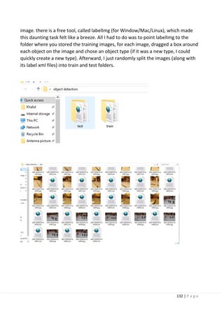
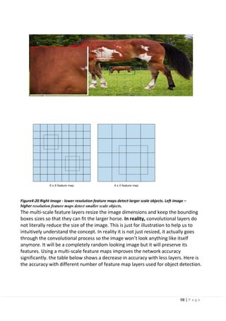
134. 133 | P a g e
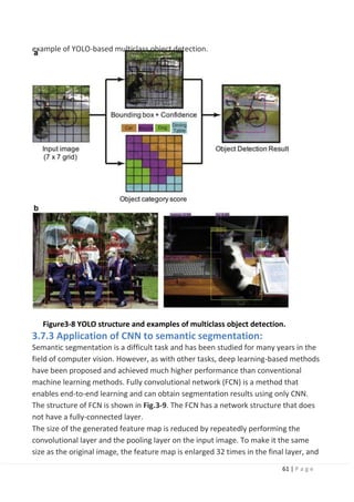
5.2.1 Model selection (most bored):
On a Raspberry Pi, since we have limited computing power, we have to choose a
model that both runs relatively fast and accurately. After experimenting with a few
models, we have settled on the MobileNet v2 SSD COCO model as the optimal
balance between speed and accuracy.
Note:
we tried faster_rcnn_inception_v2 _coco it was very accurate but very slow and we
also tried YOLO_V3 it was very fast but extremely low accuracy and its training
process is very complex.
Furthermore, for our model to work on the Edge TPU accelerator, we have to
choose the MobileNet v2 SSD COCO Quantized model.
Quantization is a way to make model inferences run faster by storing the model
parameters not as double values, but as integral values so decrease the required
memory and computational power, with very little degradation in prediction
accuracy[2]
. Edge TPU hardware is optimized and can only run quantized models.
Also if you run this quantized model on PC or laptop it will increase the speed which
is an important factor in real time object detection.

135. 134 | P a g e
Our model is :
Model name: 'ssd_mobilenet_v2_quantized_300x300_coco_2019_01_03'
pipeline_file: 'ssd_mobilenet_v2_quantized_300x300_coco.config',
batch_size: 12
5.2.2 Transfer Learning/Model Training/Testing:
For this step, we will use Google Colab again. This section is based on Chengwei’s
excellent tutorial on “How to train an object detection model easy for free”.
I will present the key parts of my Jupyter Notebook below.
Section 1: Mount Google drive
Mount my Google Drive and save modeling output files (.ckpt) there, so that it
won't be wiped out when colab Virtual Machine restarts. It has an idle timeout of
90 min, and maximum daily usage of 12 hours.
Google will ask for an authenticate code when you run the following code, just
follow the link in the output and allow access. You can put the model_dir anywhere
in your google drive.
You should create this path in your google drive or you will get an error
Section 2: Configs and Hyperparameters
Support a variety of models, you can find more pretrained model from Tensorflow
detection model zoo: COCO-trained models, as well as their pipline config files
in object_detection/samples/configs/.
we have discussed what is “ssd_mobilenet_v2_quantized” referred to.
300X300 referred to the input image size so that we will need to resize image when
using model in testing or detection after training.
Coco_2019_01_03 : referred to the datasets it trained on at first

136. 135 | P a g e
Pipeline file contain hyperparameters values such as type of optimizer and the
learning rate…etc. we will see its content later.
Section 3: Set up Training Environment
Install required packages:

137. 136 | P a g e
These packages are modules and libraries that will be used in training process.
Prepare tfrecord files:
After running this step, you will have two files train. record and test. record, both
are binary files with each one containing the encoded jpg and bounding box
annotation information for the corresponding train/test set so that TensorFlow can
process quickly. The tfrecord file format is easier to use and faster to load during
the training phase compared to storing each image and annotation separately.
There are two steps in doing so:
• Converting the individual *.xml files to a unified *.csv file foreach
set(train/test).
• Converting the annotation *.csv and image files of each
set(train/test) to *.record files (TFRecord format).
Use the following scripts to generate the tfrecord files as well
as the label_map.pbtxt file

138. 137 | P a g e
Download Pre-trained Model
Figure5-10 Download pre-trained model.
The above code will download the pre-trained model files
for ssd_mobilenet_v2_quantized_300x300_coco_2019_01_03 model and we will
only use the model.ckpt file from which we will apply transfer learning.
Section 4: Transfer Learning Training:
Configuring a Training Pipeline To do the transfer learning training, we first
downloaded the pre-trained model weights/checkpoints and then config the
corresponding pipeline. config file to tell the trainer about the following information.
• the pre-trained model checkpoint path(fine_tune_checkpoint),
• the path to those two tfrecord files,

139. 138 | P a g e
• path to the label_map.pbtxt file(label_map_path),

140. 139 | P a g e
• training batch size(batch_size)
• number of training steps(num_steps)
• number of classes of unique objects(num_classes)
• the type of optimizer()
• learning rate.

141. 140 | P a g e
Figure5-11 Part of config file indicate the batch size, optimizer type and learning rate (which is
vary in this case).
Figure5-12 Part of config file the contains information about image
resizer to make image suitable to CNN make it (300x300) and
architecture of box predictor CNN which include regularization and
drop out to avoid overfitting.

142. 141 | P a g e
During training, we can monitor the progression of loss and precision via Tensor
Board. We can see for the test dataset that loss was dropping and precision was
increasing throughout the training, which is a great sign that our training is working
as expected.
Total Loss (lower right) keeps on dropping

143. 142 | P a g e
Figure5-13 mAP (top left), a measure of precision, keeps on
increasing.
Test the Trained Model
After the training, we ran a few images from the test dataset through our new
model. As expected, almost all the objects in the image were identified with
relatively high confidence. There were a few images that objects in them were
further away, and were not detected. That’s fine for our purpose because we only
wanted to detect nearby objects so we could respond to them. The further away
objects would become larger and easier to detect as our car approached them.
The accuracy was about 92%.

144. 143 | P a g e
Code and results of testing:

145. 144 | P a g e

146. 145 | P a g e

147. 146 | P a g e
The printed number represent the distance of the object from the camera which will be
used to decide when to take the decision.
Problems:
We used our laptops to run the model on the received image from pi camera but there
was some delay due to the transmission from pi to laptop via the socket on LAN
To solve this problem, we need to buy TPU but this component not available in Egypt.

148. 147 | P a g e
Figure5-14 Google edge TPU.
we will take a look on the TPU and explain why is it important and will help??
5.3 Google’s Edge TPU. What? How? Why?
The Edge TPU is basically the Raspberry Pi of machine learning. It’s a device that
performs inference at the Edge with its TPU.
Cloud vs Edge:
Running code in the cloud means that you use CPUs, GPUs and TPUs of a company
that makes those available to you via your browser.
The main advantage of running code in the cloud is that you can assign the necessary
amount of computing power for that specific code (training large models can take a lot
of computation).
The edge is the opposite of the cloud. It means that you are running your code on
premise (which basically means that you are able to physically touch the device the
code is running on).
The main advantage of running code on the edge is that there is no network latency. As
IoT devices usually generate frequent data, running code on the edge is perfect for IoT
based solutions.

149. 148 | P a g e
Figure5-15 CPU vs GPU vs TPU.
A TPU (Tensor Processing Unit) is another kind of processing unit like a CPU or a GPU.
There are, however, some big differences between those. The biggest difference is that a
TPU is an ASIC, an Application-Specific Integrated Circuit). An ASIC is optimized to
perform a specific kind of application. For a TPU this specific task is performing multiply-
add operations which are typically used in neural networks. As you probably know, CPUs
and GPUs are not optimized to do one specific kind of application so these are not ASICs.
A CPU performs the multiply-add operation by reading each input and weight from
memory, multiplying them with its ALU (the calculator in the figure above), writing them
back to memory and finally adding up all the multiplied values.
Modern CPUs are strengthened by a massive cache, branch prediction and high clock
rate on each of its cores. Which all contribute to a lower latency of the CPU.A GPU does
the same thing but has thousands of ALU’s to perform its calculations. A calculation can
be parallelised over all ALU’s. This is called a SIMD and a perfect example of this is the
multiply -add operation in neural networks. A GPU does however not use the fancy
features which lower the latency (mentioned above). It also needs to orchestrate its
thousands of ALU’s which further decreases the latency. In short, aGPU
drastically increases its throughput by parallelizing its computation in exchange for
an increase in its latency.
A TPU, on the other hand, operates very differently. Its ALU’s are directly connected to
each other without using the memory. They can directly give pass information which will
drastically decrease latency.

150. 149 | P a g e
Performance
As a comparison, consider this:
• CPU can handle tens of operation percycle.
• GPU can handle tens of thousands of operations per cycle.
• TPU can handle up to 128000 operations per cycle.
Purpose
• Central Processing Unit (CPU): A processor designed to solve every computational
problem in a general fashion. The cache and memory design is designed to be
optimal for any general programming problem.
• Graphics Processing Unit (GPU): A processor designed to accelerate the rendering
of graphics.
• Tensor Processing Unit (TPU): A co-processor designed to accelerate deep learning
tasks develop using TensorFlow (a programming framework); Compilers have not
been developed for TPU which could be used for general purpose programming;
hence, it requires significant effort to do general programming onTPU.
Usage
• Central Processing Unit (CPU): General purpose programmingproblem.
• Graphics Processing Unit (GPU): Graphics rendering, Machine Learning model.
training and inference, efficient for programming problem with parallelization
scope, General purpose programming problem.
• Tensor Processing Unit (TPU): Machine Learning model (only in TensorFlow model)
training and inference.
Manufacturers
• Central Processing Unit (CPU): Intel, AMD, Qualcomm, NVIDIA, IBM, Samsung,
Hewlett-Packard, VIA, Atmel and many others.
• Graphics Processing Unit (GPU): NVIDIA, AMD, Broadcom Limited, Imagination
Technologies (PowerVR).
• Tensor Processing Unit (TPU): Google

151. 150 | P a g e
Figure5-14 Google edge TPU.
Quantization
A last important note on TPUs is quantization. Since Google’s Edge TPU uses 8-bit
weights to do its calculations while typically 32-bit weights are uses we should be able to
convert weights from 32 bits to 8 bits. This process is called quantization. Quantization
basically rounds the more accurate 32-bit number to the nearest 8-bit number. This
process is visually shown in the figure below.
Figure5-15 Quantization.
By rounding numbers, accuracy decreases. However, neural networks are very good in
generalization (e.g. dropout) and therefore do not take a big hit when quantization is
applied as shown in the figure below.

152. 151 | P a g e
Figure5-16 Accuracy of non-quantized model vs quantized models.
The advantages of quantization are more significant. It reduces computation and
memory needs which leads to more energy efficientcomputation.

153. 152 | P a g e
Lane Keeping System
Chapter 6

154. 153 | P a g e
6.1 Introduction
Currently, there are a few 2018–2019 cars on the market that have these two
features onboard, namely, Adaptive Cruise Control (ACC) and some forms of Lane
Keep Assist System (LKAS). Adaptive cruise control uses radar to detect and keep a
safe distance with the car in front of it. This feature has been around since around
2012–2013. Lane Keep Assist System is a relatively new feature, which uses a
windshield mount camera to detect lane lines, and steers so that the car is in the
middle of the lane. This is an extremely useful feature when you are driving on a
highway, both in bumper-to-bumper traffic and on long drives. When my family
drove from Chicago to Colorado on a ski trip during Christmas, we drove a total of 35
hours. Our Volvo XC 90, which has both ACC and LKAS (Volvo calls it PilotAssit) did an
excellent job on the highway, as 95% of the long and boring highway miles were
driven by our Volvo! All I had to do was to put my hand on the steering wheel (but
didn’t have to steer) and just stare at the road ahead. I didn’t need to steer, break, or
accelerate when the road curved and wound, or when the car in front of us slowed
down or stopped, not even when a car cut in front of us from another lane. The few
hours that it couldn’t drive itself was when we drove through a snowstorm whenlane
markers were covered by snow. (Volvo, if you are reading this, yes, I will take
endorsements! :) Curious as I am, I thought to myself: I wonder how this works, and
wouldn’t it be cool if I could replicate this myself (on a smaller scale)?
we will build LKAS into our DeepPiCar. Implementing ACC requires a radar, which our
PiCar doesn’t have. In a future article, I may add an ultrasonic sensor on DeepPiCar.
Ultrasound, similar to radar, can also detect distances, except at closer ranges, which
is perfect for a small-scale robotic car.
6.2 Timeline of available systems
1992: Mitsubishi Motors began offering a camera-assisted lane-keeping support
system on the Mitsubishi Debonair sold in Japan.
2001: Nissan Motors began offering a lane-keeping support system on the Cima sold in
Japan.
2002: Toyota introduced its Lane Monitoring System on models such as the Cardina
and Alphard sold in Japan; this system warns the driver if it appears the vehicle is
beginning to drift out of its lane.
In 2004, Toyota added a Lane Keeping Assist feature to the Crown Majesta which
can apply a small counter-steering force to aid in keeping the vehicle in its lane.
In 2006, Lexus introduced a multi-mode Lane Keeping Assist system on the LS

155. 154 | P a g e
460, which utilizes stereo cameras and more sophisticated object- and pattern-
recognition processors. This system can issue an audiovisual warning and also
(using the Electric Power Steering or EPS) steer the vehicle to hold its lane. It also
applies counter-steering torque to help ensure the driver does not over-correct
or "saw" the steering wheel while attempting to return the vehicle to its proper
lane. If the radar cruise control system is engaged, the Lane Keep function works
to help reduce the driver's steering-input burden by providing steering torque;
however, the driver must remain active or the system will deactivate.
2003: Honda launched its Lane Keep Assist System (LKAS) on the Inspire. It provides
up to 80% of steering torque to keep the car in its lane on the highway. It is also
designed to make highway driving less cumbersome, by minimizing the driver's
steering input. A camera, mounted at the top of the windshield just above the rear-
view mirror, scans the road ahead in a 40-degree radius, picking up the dotted white
lines used to divide lane boundaries on the highway. The computer recognizes that
the driver is "locked into" a particular lane, monitors how sharp a curve is and uses
factors such as yaw and vehicle speed to calculate the steering input required.
2004: In 2004, the first passenger-vehicle system available in North America was
jointly developed by Iteris and Valeo for Nissan on the Infiniti FX and (in 2005) the
M vehicles. In this system, a camera (mounted in the overhead console above the
mirror) monitors the lane markings on a roadway. A warning tone is triggered to
alert the driver when the vehicle begins to drift over the markings.
2005: Citroën became the first in Europe to offer LDWS on its 2005 C4 and C5 models,
and its C6. This system uses infrared sensors to monitor lane markings on the road
surface, and a vibration mechanism in the seat alerts the driver of deviations.
2007: In 2007, Audi began offering its Audi Lane Assist feature for the first time on
the Q7. This system, unlike the Japanese "assist" systems, will not intervene in
actual driving; rather, it will vibrate the steering wheel if the vehicle appears to be
exiting its lane. The LDW System in Audi is based on a forward-looking video-
camera in its visible range, instead of the downward-looking infrared sensors in the
Citroën. Also, in 2007, Infiniti offered a newer version of its 2004 system, which it
called the Lane Departure Prevention (LDP) system. This feature utilizes the vehicle
stability control system to help assist the driver maintain lane position by applying
gentle brake pressure on the appropriate wheels.

156. 155 | P a g e
2008: General Motors introduced Lane Departure Warning on its 2008 model-year
Cadillac STS, DTS and Buick Lucerne models. The General Motors system warns the
driver with an audible tone and a warning indicator on the dashboard. BMW also
introduced Lane Departure Warning on the 5 series and 6 series, using a vibrating
steering wheel to warn the driver of unintended departures. In late 2013 BMW
updated the system with Traffic Jam Assistant appearing first on the redesigned X5,
this system works below 25mph. Volvo introduced the Lane Departure Warning system
and the Driver Alert Control on its 2008 model-year S80, the V70 and XC70 executive
cars. Volvo's lane departure warning system uses a camera to track road markings and
sound an alarm when drivers depart them. lane without signaling. The systems used
by BMW, Volvo and General Motors are based on core technology from Mobileye.
2009: Mercedes-Benz began offering a Lane Keeping Assist function on the new E-
class. This system warns the driver (with a steering-wheel vibration) if it appears the
vehicle is beginning to leave its lane. Another feature will automatically deactivate
and reactivate if it ascertains the driver is intentionally leaving his lane (for instance,
aggressively cornering). A newer version will use the braking system to assist in
maintaining the vehicle's lane. In 2013 on the redesigned S-class Mercedes began
Distronic Plus with Steering Assist and Stop &Go Pilot.
2010: Kia Motors offered the 2011 Cadenza premium sedan with an optional Lane
Departure Warning System (LDWS) in limited markets. This system uses a flashing
dashboard icon and emits an audible warning when a white lane marking is being
crossed, and emits a louder audible warning when a yellow-line marking is crossed.
This system is canceled when a turn signal is operating, or by pressing a deactivation
switch on the dashboard; it works by using an optical sensor on both sides of the car.
Fiat is also launching its Lane Keep Assist feature based on TRW's lane keeping assist
system (also known as the Haptic Lane Feedback system). This system integrates the
lane- detection camera with TRW's electric power-steering system; when an
unintended lane departure is detected (the turn signal is not engaged to indicate the
driver's desire to change lanes), the electric power- steering system will introduce a
gentle torquethat will help guide the driver back toward the center of the lane.
Introduced on the Lancia Delta in 2008, this system earned the Italian Automotive
Technical Association's Best Automotive Innovation of the Year Award for 2008.
Peugeot introduced the same system as Citroën in its new 308.

157. 156 | P a g e
6.3 Current lane keeping system in market
Many automobile manufacturers provide optional lane keeping systems including
Nissan, Toyota, Honda, General Motors, Ford, Tesla, and many more. However,
these systems require human monitoring and acceleration/deceleration inputs are
not completely automatic. Ford’s system4 uses a single camera mounted behind
the windshield’s rear-view mirror to monitor the road lane markings. The system
can only be used when driving above 40 mph and is detecting at least one lane
marking. When the system is active, it will alert the driver if they are drifting out
of lane or provide some steering torque towards the lane center. If thesystem
detects no steering activity for a short period, the system will alert the driver to put
their hands on the steering wheel. The lane keeping system can also be temporarily
suppressed by certain actions such as quick braking, fast acceleration, use of the
turn signal indicator, or an evasive steering maneuver. Ford’s system also allows the
choice between alerting, assisting, or both when active. All these systems use
similar strategies in aiding a human driver to stay in lane, but do not allow full
autonomous driving4-7. GM, in particular, warns that their lane keeping system
should not be used while towing a trailer or on slippery roads, as it could cause loss
of control of the vehicle and a crash5.
6.4 overview of lane keeping algorithms
The camera and radar system detect the relationship between the vehicle
position and the lane mark and then send this information to the lane departure
warning algorithm.
The algorithm integrates sensors’ information, the GPS position information and
the vehicle state information. Most of the published literature on LDWS and LKAS
uses visual sensors to obtain lane line information, and combined with warning
decision algorithms to identify whether the vehicle has a tendency to departure

158. 157 | P a g e
from the original lane. The lane departure warning algorithms used by various
research institutions are basically divided into two categories, one is the
combination of road structure model and image information, and the other is
only using image information. There are eight types of departure warning
algorithms that are currently used commonly: TLC algorithm, FOD algorithm, CCP
algorithm, instantaneous lateral displacement algorithm, lateral velocity
algorithm, Edge Distribution Function (EDF) algorithm, and Time to Trajectory
Divergence (TTD) algorithm and Road Rumble Strips (RRS) algorithm. The RRS
algorithm belongs to the combination of road structure and image information,
which requires the installation of vibration bands or constructing new roads.
In the existing road, a 15cm~45cm groove is placed on the shoulder of the road. If
the vehicle deviates from the lane and enters the groove, the tire will rub against
the groove due to contact, and the sound of the friction will remind the driver the
departure from the original lane. The seven departure warning algorithms except
RRS belong to the algorithm using only image information. In order to clearly
understand the advantages and disadvantages of various algorithms, and to guide
the study of the lane departure warning algorithm, the comparative analysis of the
above eight warning algorithms is shown in table:

159. 158 | P a g e
Algorithms Pros Cons
TLC Long warning time Fixed parameter
FOD Multiple warning
thresholds
Limited reaction time
for driver
CCP Based on real-time position High precision sensor
Literal velocity Easy to define High false rate
TTD Always flow lane center Complex algorithm and
works bad in bend
Instantaneous
Lateral
Displacement
Simple algorithm and
easy to realize
Ignored the vehicle
trajectory, relativelyhigh
false rate
EDF No need for camera Complex algorithm
RRS Effective alert High cost
Figure6.1 the lane departure warning algorithm
From the above analysis, it is clear that each algorithm has different advantages and
disadvantages. The eight common departure warning algorithms have certain
limitations and the algorithm does not change once it is determined. But factors such
as age, gender, and driving age make each driver almost have their own driving habits.
Therefore, the efficient and practical warning algorithm must not only have higher
precision, but also should adapt to the driving habits of different types of drivers.
Among the above methods, TLC has simple using conditions and high precision, and is
the most widely used in LDWS and LKAS related products.
FOD considers driving habits when setting the lane virtual boundary line, but the
accuracy is limited. Therefore, in order to make LKAS adapt to different types of

160. 159 | P a g e
drivers to the maximum extent, this paper improves the existing TLC and FOD
algorithms—establishing TLC and FOD algorithms with selectable mode and multiple
working conditions and based on them, and proposes the concept of dynamic warning
boundary and warning parameters.
The FOD algorithm originally matched driver habits by setting different virtual lane
boundaries. The design of this paper considers the impact of the surrounding traffics,
and is more adaptive with diverse driving habits. The driver can choose the appropriate
LKAS working mode and warning boundary based on personal driving habits and the
experience of LKAS.
6.5 Perception: Lane Detection
A lane keeps assist system has two components, namely, perception (lane detection)
and
Path/Motion Planning (steering). Lane detection’s job is to turn a video of the road into
the
coordinates of the detected lane lines. One way to achieve this is via the computer
vision package. But before we can detect lane lines in a video, we must be able to
detect lane lines in a single image. Once we can do that, detecting lane lines in a video
is simply repeating the same steps for all frames in a video. There are many steps.
1- Isolate the Color of the Lane:
When I set up lane lines for my DeepPiCar in my living room, I used the blue painter’s
tape to mark the lanes, because blue is a unique color in my room, and the tape won’t
leave permanent sticky residues on the hardwood floor.
The first thing to do is to isolate all the blue areas on the image. To do this, we first need
to turn the color space used by the image, which is RGB (Red/Green/Blue) into the HSV
(Hue/Saturation/Value) color space. (Read this for more details on the HSV color space.)
The main idea behind this is that in an RGB image, different parts of the blue tape may
be lit with different light, resulting them appears as darker blue or lighter blue.
However, in HSV color space, the Hue componentwill render the entire blue tape as one
color regardless of its shading. It is best to illustrate with the following image. Notice
both lane lines are now roughly the same magenta color.

161. 160 | P a g e
Figure6.2 Image in HSV Color
Below is the OpenCV command to do this.
Figure6.3 OpenCV command
Note that we used a BGR to HSV transformation, not RBG to HSV. This is because
OpenCV, for some legacy reasons, reads images into BGR (Blue/Green/Red) color space
by default, instead of the more commonly used RGB (Red/Green/Blue) color space.
They are essentially equivalent color spaces, just order of the colors swapped.
Once the image is in HSV, we can “lift” all the blueish colors from the image. This is by
specifying a range of the color Blue.
In Hue color space, the blue color is in about 120–300 degrees range, on a 0–360
degrees scale. You can specify a tighter range for blue, say 180–300 degrees, but it
doesn’t matter too much.
Figure6.4 Hue in 0-360 degrees scale
Here is the code to lift Blue out via OpenCV, and rendered maskimage.
Figure6.5 code to lift Blue out via OpenCV, and rendered maskimage.

162. 161 | P a g e
Blue area mask
Note
OpenCV uses a range of 0–180, instead of 0–360, so the blue range we need to
specify in OpenCV is 60–150 (instead of 120–300). These are the first parameters
of the lower and upper bound arrays. The second (Saturation) and third
parameters (Value) are not so important, I have found that the 40–255 ranges
work reasonably well for both Saturation and Value.
Note
this technique is exactly what movie studios and weatherperson use every day. They
usually use a green screen as a backdrop, so that they can swap the green color with
a thrilling video of a T- Rex charging towards us (for a movie), or the live doppler
radar map (for the weatherperson).
2- Detecting Edges of Lane Lines:
we need to detect edges in the blue mask so that we can have a few distinct lines that
represent the blue lane lines.
The Canny edge detection function is a powerful command that detects edges in an
image. In the code below, the first parameter is the blue mask from the previous step.
The second and third parameters are lower and upper ranges for edge detection,
which OpenCV recommends to be (100, 200) or (200, 400), so we are using (200, 400).
Figure6.6 OpenCV recommends.

163. 162 | P a g e
Figure6.7 Edges of all Blue Areas.
3- Isolate Region of Interest:
From the image above, we see that we detected quite a few blue areas that areNOT
our lane lines. A closer look reveals that they are all at the top half of thescreen.
Indeed, when doing lane navigation, we only care about detecting lane lines that are
closer to the car, where the bottom of the screen. So, we will simply crop out the
top half. Boom! Two clearly marked lane lines as seen on the image on the right!
Figure6.8 Cropped Edges.
Here is the code to do this. We first create a mask for the bottom half of the screen.
Then when we merge the mask with the edges image to get the cropped edges image
on the right.

164. 163 | P a g e
4- Detect Line Segments:
In the cropped edges image above, to us humans, it is pretty obvious that we found
four lines, which represent two lane lines. However, to a computer, they are just a
bunch of white pixels on a black background. Somehow, we need to extract the
coordinates of these lane lines from these white pixels. Luckily, OpenCV contains a
magical function, called Hough Transform, which does exactly this. Hough Transform is
a technique used in image processing to extract features like lines, circles, and ellipses.
We will use it to find straight lines from a bunch of pixels that seem to form a line. The
function Hough Lines essentially tries to fit many lines through all the white pixels and
return the most likely set of lines, subject to certain minimum threshold constraints.
(Read here for an in-depth explanation of Hough LineTransform.)
Here is the code to detect line segments. Internally, Hough Line detects lines using
Polar Coordinates. Polar Coordinates (elevation angle and distance from the origin) is
superior to Cartesian Coordinates (slope and intercept), as it can represent any lines,
including vertical lines which Cartesian Coordinates cannot because the slope of a
vertical line is infinity. Hough Line takes a lot of parameters:
1) rho is the distance precision in pixel. We will use one pixel.
2) angle is angular precision in radian. (Quick refresher on Trigonometry:
radian is another way to express the degree of angle. i.e. 180 degrees in radian is
3.14159, which is π) We will use one degree.
3) Min threshold is the number of votes needed to be considered a line

165. 164 | P a g e
segment. If a line has more votes, Hough Transform considers them tobe
more likely to have detected a line segment.
4) Min LineLength is the minimum length ofthe line segment in pixels. Hough
Transformwon’t return any line segments shorter than this minimum length.
5)maxLineGap is the maximum in pixels that two-line segments that canbe
separated and still be considered a single line segment.
For example, if we had dashed lane markers, by specifying a reasonable max line gap,
Hough Transform will consider the entire dashed lane line as one straight line, which is
desirable. Setting these parameters is really a trial and error process. Below are the
values that worked well for my robotic car with a 320x240 resolution camera running
between solid blue lane lines. Of course, they need to be re-tuned for a life-sized car
with a high-resolution camera running on a real road with white/yellow dashed lane
lines.
Figure6.9 Line segments detected by Hough Transform
Combine Line Segments into Two Lane Lines:
Now that we have many small line segments with their endpoint coordinates (x1, y1)
and (x2, y2), how do we combine them into just the two lines that we really care

166. 165 | P a g e
about, namely the left and right lane lines? One way is to classify these line segments
by their slopes. We can see from the picture above that all line segments belonging to
the left lane line should be upward sloping and on the left side of the screen, whereas
all line segments belonging to the right lane line should be downward sloping and be
on the right side of the screen. Once the line segments are classified into two groups,
we just take the average of the slopes and intercepts of the line segments to get the
slopes and intercepts of left and right lane lines.
The average_slope_intercept function below implements the above logic.

167. 166 | P a g e
Make points is a helper function for the average_slope_intercept function, which takes
a line’s slope and intercept, and returns the endpoints of the line segment.
Other than the logic described above, there are a couple of special cases worth
discussion.
1. One lane line in the image:
In normal scenarios, we would expect the camera to see both lane lines.
However, there are times when the car starts to wander out of the lane,
maybe due to flawed steering logic, or when the lane bends too sharply. At
this time, the camera may only capture one lane line. That’s why the code
above needs to check len(right-fit)>0 and len(left-fit)>0.
2. Vertical line segments:
vertical line segments are detected occasionally as the car is turning. Although
they are not erroneous detections, because vertical lines have a slope of
infinity, we can’t average them with the slopes of other line segments. For
simplicity’s sake, I chose to just to ignore them. As vertical lines are not very
common, doing so does not affect the overall performance of the lane
detection algorithm. Alternative, one could flip the X and Y coordinates of the
image, so vertical lines have a slope of zero, which could be included in the
average. But then the horizontal line segments would have a slope of infinity,
but that would be extremely rare, since the DashCam is generally pointing at
the same direction as the lane lines, not perpendicular to them. Another
alternative is to represent the line segments in polar coordinates and then
averaging angles and distance to the origin.

168. 167 | P a g e
6.6 Motion Planning: Steering
Now that we have the coordinates of the lane lines, we need to steer the carso
that it will stay within the lane lines, even better, we should try to keep it inthe
middle of the lane. Basically, we need to compute the steering angle of the car,
given the detected lane lines.
Two Detected Lane Lines:
This is the easy scenario, as we can compute the heading direction by simply
averaging the far endpoints of both lane lines. The red line shown below is the
heading. Note that the lower end of the red heading line is always in the middle of
the bottom of the screen, that’s because we assume the dashcam is installed in the
middle of the car and pointing straight ahead.
One Detected Lane Line:
If we only detected one lane line, this would be a bit tricky, as we can’t do an
average of two endpoints anymore. But observe that when we see only one lane
line, say only the left (right) lane, this means that we need to steer hard towards the
right(left), so we can continue to follow the lane. One solution is to set the heading
line to be the same slope as the only lane line, as shown below.

169. 168 | P a g e
Steering Angle:
Now that we know where we are headed, we need to convert that into the steering
angle, so that we tell the car to turn. Remember that for this PiCar, thesteering angle
of 90 degrees is heading straight, 45–89 degrees are turning left, and 91–135
degrees is turning right. Below is some trigonometry to convert a heading coordinate
to a steering angle in degrees. Note that PiCar is created for common men, so it uses
degrees and not radians. But all trig math is done in radians.
Displaying Heading Line:
We have shown several pictures above with the heading line. Here is the code that
renders it. The input is actually the steering angle.
Stabilization:
Initially, when I computed the steering angle from each video frame, I simply told the
PiCar to steer at this angle. However, during actual road testing, I have found that
the PiCar sometimes bounces left and right between the lane lines like a drunk
driver, sometimes go completely out of the lane. I then found out that it is caused by

170. 169 | P a g e
the steering angles, computed from one video frame to the next frame, are not very
stable. You should run your car in the lane without stabilization logic to see what I
mean. Sometimes, the steering angle may be around 90 degrees (heading straight)
for a while, but, for whatever reason, the computed steering angle could suddenly
jump wildly, to say 120 (sharp right) or 70 degrees (sharp left). As a result, the car
would jerk left and right within the lane. Clearly, this is not desirable.
We need to stabilize steering. Indeed, in real life, we have a steering wheel, so that if
we want to steer right, we turn the steering wheel in a smooth motion, and the
steering angle is sent as a continuous value to the car, namely, 90, 91, 92, …. 132,
133, 134, 135 degrees, not 90 degrees in one millisecond, and 135 degrees in next
millisecond.
So, my strategy to stable steering angle is the following: if the new angle is more
than max_angle_deviation degree from the current angle, just steer up to
max_angle_deviation degree in the direction of the new angle.
we used two flavors of max_angle_deviation, 5 degrees if both lane lines are
detected, which means we are more confident that our heading is correct; 1 degree
if only one lane line is detected, which means we are less confident. These are
parameters one can tune for his/her own car.

171. 170 | P a g e
6.7 Lane keeping via Deep Learning
we hand engineered all the steps required to navigate the car, i.e. color isolation,
edge detection, line segment detection, steering angle computation, and steering
stabilization. Moreover, there were quite a few parameters to hand tune, such as
upper and lower bounds of the color blue, many parameters to detect line segments
via Hough Transform, and max steering deviation during stabilization, etc. If we
didn’t tune all these parameters correctly, our car wouldn’t run smoothly.
Moreover, every time we had new road conditions, we would have to think of new
detection algorithms and program them into the car, which is very timeconsuming
and hard to maintain. In the era of AI and machine learning.
The Nvidia Model:
At the high level, the inputs to the Nvidia model are video images from Dashcams
onboard the car, and outputs are the steering angle of the car. The model uses the
video images, exacts information from them, and tries to predict the car’s steering
angles. This is known as a supervised machine learning program, where video images
(called features) and steering angles (called labels) are used in training. Because the
steering angles are numerical values, this is a regression problem, instead of a
classification problem, where the model needs to predict if a dog or a cat, or which
one type of flower is the in the image.
At the core of the NVidia model, there is a Convolutional Neural Network (CNN,
not the cable network). CNNs are used prevalently in image recognition deep
learning models. The intuition is that CNN is especially good at extracting visual
features from images from its various layers (aka. filters). For example, for a facial
recognition CNN model, the earlier layers would extract basic features, such as line
and edges, middle layers would extract more advanced features, such as eyes
noses, ears, lips, etc. and later layers would extract part or all of a face.

172. 171 | P a g e
Figure6.9 CNN architecture.
CNN architecture. The network has about 27 million connections and
250 thousand parameters.
The above diagram is from Nvidia’s paper. It contains about 30 layers in total, not a
very deep model by today’s standards. The input image to the model (bottom of the
diagram) is a 66x200 pixel image, which is a pretty low-resolution image. The image
is first normalized, then passed
through 5 groups of convolutional layers, finally passed through 4 fully connected
neural layers and arrived at a single output, which is the model predictedsteering
angle of the car.

173. 172 | P a g e
Figure6.10 Method of Training.
This model predicted angle is then compared with the desired steering angle giventhe
video image, the error is fed back into the CNN training process via backpropagation.
As seen from the diagram above, this process is repeated in a loop until the errors
(aka loss or Mean Squared Error) is low enough, meaning the model has learned how
to steer reasonably well. Indeed, this is a pretty typical image recognition training
process, except the predicted output is a numerical value (regression) instead of the
type of an object (classification).
Adapting the Nvidia Model for DeepPiCar:
Other than in size, our DeepPiCar is very similar to the car that Nvidia uses, in that it
has a Dashcam, and it can be controlled by specifying a steering angle. Nvidia
collected its inputs by having its drivers drove a combined 70 hours of highway
miles, in various states and multiple cars. So, we need to collect some video footage
of our DeepPiCar and record the correct steering angle for each video image.
Data Acquisition:
write a remote-control program so that we can remotely steer the PiCar, and have it
saved down the video frame as well as the car’s steering angles at each frame. This is
probably the best way since it would be simulating a real person’s driving behavior.

174. 173 | P a g e
Figure6.11 Angles distribution from Data acquisition.
Here is the code to take a video file and save down the individual video frames for
training. For simplicity, I embed the steering angle as part of the image file name, so I
don’t have to maintain a mapping file between image names and steering angles.

175. 174 | P a g e
Training/Deep Learning:
Now that we have the features (video images) and labels (steering angles), it is time
to do some deep learning! In fact, this is the first time in this DeepPiCar blog series
that we are doing deep learning. Even though Deep Learning is all the hype these
days, it is important to note it is just a small part of the whole engineering project.
Most of the time/work is actually spend on hardware engineering, software
engineering, data gathering/cleaning, and finally wire up the predictions of the
deep learning models to production systems (like a running car), etc.
To do deep learning model training, we can’t use the Raspberry Pi’s CPU, and we need
some GPU muscle! Yet, we are on a shoestring budget, so we don’t want to pay for an
expensive machine with the latest GPU, or rent GPU time from the cloud. Luckily,
Google offers some of GPU and even TPU power for FREE on this site called Google
Colab! Kudos to Google for giving us machine learning enthusiasts a great playground
to learn.
Split into Train/Test Set
We will split the training data into training/validation sets with a 80/20 split with
sklearn’s
train_test_split method.
Image Augmentation:
The sample training data set only has about 200 images. Clearly, that’s not enough
to train our deep learning model. However, we can employ a simple technique,
called Image Augmentation. Some of the common augmentation operations are
zooming, panning, changing exposure values, blurring, and imaging flipping. By
randomly applying any or all of these 5 operations on the original images, we can
generate a lot more training data from our original 200 images, which makes our
final trained model much more robust.

176. 175 | P a g e
6.8 Google Colab for Training:
1-mount google drive to colab to import our Training and testing Data:
Figure 6.12 mount Drive to colab.
2-import package we need it:
Figure 6.13 python package for training.
3-Loading Data from Drive:
Figure 6.14 Loading our data from drive.

177. 176 | P a g e
4-Training and testing data distribution:
Figure 6.15 train and test data.
5-prepare Nvidia model:
Figure 6.16 load model.
Figure 6.17 Summary Model.

178. 177 | P a g e
6-Evaluate the Trained Model:
After training for 30 min, the model will finish the 10 epochs. Now it is time to see how well the
training went. First thing is to plot the loss function of both training and validation sets. It is good to
see that both training and validation losses declined rapidly together, and then stayed very low after
epoch 5. There didn’t seem to be any overfitting issue, as validation loss stayed low with training loss.
Figure6.18 Graph of training and validation loss.
Figure6.19 Result of our model on our data.

179. 178 | P a g e
System Integration
Chapter 7

180. 179 | P a g e
Laptop
Raspberry-pi
Arduino
7.1 introduction:
now we need to connect our systems together. First we need to make
connection between raspberry-pi and laptop to send the images will be
taken from raspberry-pi camera to laptop to make processing on it to make
a decision second, we make connection between raspberry pi and Arduino
to send our decision to Arduino and Arduino implement it with the others
components.
Figure7-1 Diagram for connections.
7.2 connection between laptop and raspberry-pi:
Now we need stable and high-speed wireless connection so we have to
choose TCP connection because TCP connection has some advantages which
we need like TCP provides extensive error checking mechanisms. It is
because it provides flow control and acknowledgment of data and
Sequencing of data is a feature of Transmission Control Protocol (TCP). this
means that packets arrive in-order at the receiver. So that we cannot choose
UDP connection because we need all packets because TCP connection has
acknowledgement to ensure the packet is received, we sent to laptop to
collect the whole image we sent.
7.2.1 TCP connection:

181. 180 | P a g e
7.2.1.1 Connection establishment
To establish a connection, TCP uses a three-way handshake. Before a client
attempts to connect with a server, the server must first bind to and listen at a
port to open it up for connections: this is called a passive open. Once the
passive open is established, a client may initiate an active open.
Figure7.2 Server.
Figure7.3 Client.
Before that we record the streaming from raspberry-pi on the connection
file (Client Side) and will read the record from laptop (server side) and split
the frames and make processing on frame by frame.
Figure7.4 Recording stream on connection file.

182. 181 | P a g e
Figure7.5 Reading from connection file and Split frames on server side.
Then we will send every frame to machine learning models then get the
decision and send it to raspberry-pi again, finally we terminate the
connection.
7.2.1.2 Connection termination
The connection termination phase uses a four-way handshake, with each side
of the connection terminating independently. When an endpoint wishes to
stop its half of the connection, it transmits a FIN packet, which the other end
acknowledges with an ACK. Therefore, a typical tear-down requires a pair of
FIN and ACK segments from each TCP endpoint. After both FIN/ACK
exchanges are concluded, the side which sent the first FIN before receiving
one waits for a timeout before finally closing the connection, during which
time the local port is unavailable for new connections; this prevents
confusion due to delayed packets being delivered during subsequent
connections.
A connection can be “half-open”, in which case one side has terminated its
end, but the other has not. The side that has terminated can no longer send
any data into the connection, but the other side can. The terminating side
should continue reading the data until the other side terminates as well. It is
also possible to terminate the connection by a 3-way handshake, when host
A sends a FIN and host B replies with a FIN & ACK (merely combines 2 steps
into one) and host A replies with an ACK. This is perhaps the most common
method.
It is possible for both hosts to send FINs simultaneously then both just have
to ACK. This could possibly be considered a 2-way handshake since the
FIN/ACK sequence is done in parallel for both directions.
Some host TCP stacks may implement a half-duplex close sequence, as Linux
or HP-UX do. If such a host actively closes a connection but still has not read
all the incoming data the stack already received from the link, this host sends
a RST instead of a FIN (Section 4.2.2.13 in RFC 1122). This allows a TCP
application to be sure the remote application has read all the data the former

183. 182 | P a g e
sent— waiting the FIN from the remote side, when it actively closes the
connection. However, the remote TCP stack cannot distinguish between a
Connection Aborting RST and this Data Loss RST. Both cause the remote stack
to throw away all the data it received, but that the application still didn’t
read.
Figure7.6 Terminate connection in two sides.
Figure7.7 Operation of TCP.
7.3 connection between raspberry-pi and Arduino:
Now we need a simple connection and uses the least wires, so that
we will use i2
c (i-squared-c) protocol. This protocol needs just two
wires to make a connection and has hardware acknowledgement to
ensure the data is received.
7.3.1 I2
c (I-squared-C):
The Inter-Integrated Circuit (aka I²C - pronounced I-squared-C or very rarely I-
two-C) is a hardware specification and protocol developed by the
semiconductor division of Philips (now NXP Semiconductors³) back in 1982. It

184. 183 | P a g e
is a multi-slave⁴, half-duplex, single-ended 8-bit oriented serial bus
specification, which uses only two wires to interconnect a given number of
slave devices to a master.
Until October 2006, the development of I²C-based devices was subject to the
payment of royalty fees to Philips, but this limitation has been superseded⁵.
Figure7.8 Graphical representation of the i2
c bus.
In the I²C protocol all transactions are always initiated and completed by
the master. This is one of the few rules of this communication protocol to
keep in mind while programming (and, especially, debugging) I²C devices.
All messages exchanged over the I²C bus are broken up into two types of
frame: an address frame, where the master indicates to which slave the
message is being sent, and one or more data frames, which are 8-bit data
messages passed from master to slave or vice versa. Data is placed on the
SDA line after SCL goes low, and it is sampled after the SCL line goes high.
The time between clock edges and data read/write is defined by devices on
the bus and it vary from chip to chip. As said before, both SDA and SCL are
bidirectional lines, connected to a positive supply voltage via a current-
source or pull-up resistors (see Figure 7.8). When the bus is free, both lines
are HIGH. The output stages of devices connected to the bus must have an
open-drain or open-collector to perform.
the wired-AND function. The bus capacitance limits the number of interfaces
connected to the bus. For a single master application, the master’s SCL output
can be a push-pull driver design if there are no devices on the bus that would
stretch the clock (more about this later). We are now going to analyze the
fundamental steps of an I²C communication.

185. 184 | P a g e
Figure7.9 Structure of a base i2
c message.
Start and stop condition:
All transactions begin with a START and are terminated by a STOP (see
Figure 7.9). A HIGH to LOW transition on the SDA line while SCL is HIGH
defines a START condition. A LOW to HIGH transition on the SDA line
while SCL is HIGH defines a STOP condition.
START and STOP conditions are always generated by the master. The bus is
considered to be busy after the START condition. The bus is considered to
be free again a certain time after the STOP condition. The bus stays busy if a
repeated START (also called RESTART condition) is generated instead of a
STOP condition (more about this soon). In this case, the START and RESTART
conditions are functionally identical.
Byte format:
Every word transmitted on the SDA line must be eight bits long, and this also
includes the address frame as we will see in a while. The number of bytes
that can be transmitted per transfer is unrestricted. Each byte must be
followed by an Acknowledge (ACK) bit. Data is transferred with the Most
Significant Bit (MSB) first (see Figure 2). If a slave cannot receive or transmit
another complete byte of data until it has performed some other function,
for example servicing an internal interrupt, it can hold the clock line SCL LOW
to force the master into a wait state. Data transfer then continues when the
slave is ready for another byte of data and releases clock line SCL.
Address frame:
The address frame is always first in any new communication sequence.
For a 7-bit address, the address is clocked out most significant bit (MSB)
first, followed by a R/W bit indicating whether this is a read (1) or write
(0) operation
In a 10-bit addressing system, two frames are required to transmit the
slave address.

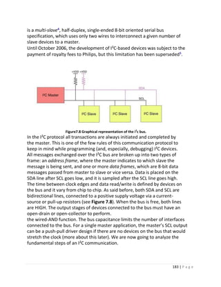
186. 185 | P a g e
The first frame will consist of the code 1111 0XXD2 where XX are the two MSB
bits of the 10-bit slave address and D is the R/W bit as described above. The
first frame ACK bit will be asserted by all slaves matching the first two bits of
the address. As with a normal 7-bit transfer, another transfer begins
immediately, and this transfer contains bits [7:0] of the address. At this point,
the addressed slave should respond with an ACK bit. If it doesn’t, the failure
mode is the same as a 7-bit system.
Note that 10-bit address devices can coexist with 7-bit address devices, since
the leading 11110 part of the address is not a part of any valid 7-bit
addresses.
Acknowledge (ACK) and Not Acknowledge (NACK):
The ACK takes place after every byte. The ACK bit allows the receiver to
signal the transmitter⁹ that the byte was successfully received and
another byte may be sent. The master generates all clock pulses over the
SCL line, including the ACK ninth clock pulse.
The ACK signal is defined as follows: the transmitter releases the SDA line
during the acknowledge clock pulse so that the receiver can pull the SDA
line LOW and it remains stable LOW during the HIGH period of this clock
pulse. When SDA remains HIGH during this ninth clock pulse, this is
defined as the Not Acknowledge (NACK) signal. The master can then
generate either a STOP condition to abort the transfer, or a RESTART
condition to start a new transfer. There are five conditions leading to the
generation of a NACK:
5.No receiver is present on the bus with the transmitted address so there
is no device to respond with an acknowledge.
6.The receiver is unable to receive or transmit because it is performing
some real-time function and is not ready to start communication with
the master.
7.During the transfer, the receiver gets data or commands that it does
not understand.
8.During the transfer, the receiver cannot receive any more data bytes.
9.A master-receiver must signal the end of the transfer to the
slave transmitter.

187. 186 | P a g e
Data Frames:
After the address frame has been sent, data can begin being transmitted.
The master will simply continue generating clock pulses on SCL at a
regular interval, and the data will be placed on SDA by either the master
or the slave, depending on whether the R/W bit indicated a read or write
operation.
Usually, the first or the first two bytes contains the address of the slave
register to write to/read from.
For example, for I²C EEPROMs the first two bytes following the address
frame represent the address of the memory location involved in the
transaction.
Depending on the R/W bit, the successive bytes are filled by the master (if
the R/W bit is set to 1) or the slave (if R/W bit is 0). The number of data
frames is arbitrary, and most slave devices will auto-increment the
internal register, meaning that subsequent reads or writes will come from
the next register in line. This mode is also called sequential or burst mode
and it is a way to speed up transfer speed.
Implementation on code:
As mentioned above in this chapter. We get the decision from laptop and
send it to raspberry-pi then we need to send the decision to Arduino using
i2
c protocol.
Figure7-10 I2c code in raspberry-pi.

188. 187 | P a g e
Figure7.11 I2
c code in Arduino.

189. 188 | P a g e
Software for connections
Chapter 8

190. 189 | P a g e
8.1 Introduction:
Self-Driving car is the most trending technology which already
implemented in Tesla cars, as initially, you can learn about the technology
by using this system. For this, we are using OpenCV, Machine learning
technology. This system contains Raspberry Pi as the core system, which
having functionalities like, Traffic light detection, Vehicle detection,
pedestrian detection, Road sign detection to make the car as autonomous.
Every process is done using the Raspberry Pi with Python programming.
BLOCK DIAGRAM
Figure 8.1 Block diagram of system

191. 190 | P a g e
8.2 Programs setup and analysis:
8.2.1 Raspberry-pi:
The Raspberry Pi is a low cost, credit-card sized computer that plugs into a
computer monitor or TV, and uses a standard keyboard and mouse. It is a
capable little device that enables people of all ages to explore computing, and
to learn how to program in languages like Scratch and Python. It is capable of
doing everything you would expect a desktop computer to do, from browsing
the internet and playing high-definition video, to making spreadsheets, word-
processing, and playing games.
Figure 8.2 (Raspberry pi).
8.2.2 component of raspberry pi:
• 4 USB ports.
• 40 GPIO pins.
• Full HDMI port.
• Ethernet port (10/100 base Ethernet socket).
• Combined 3.5mm audio jack and composite video.
• Camera interface (CSI).
• Display interface (DSI). Micro-SD card slot.
• Video Core IV 3D graphics core.
8.2.3 Hardware interfaces:
Include a UART, an I2C bus, and a SPI bus with two chip selects, I2S audio,
3V3, 5V, and ground. The maximum number of GPIOs can theoretically be
indefinitely expanded by making use of the I2C.

192. 191 | P a g e
8.2.4 Required software:
The Raspberry Pi runs off an operating system based on Linux called Raspbian.
For this project, the most recent Raspbian Jessie Lite image was installed. The
Raspberry Pi website has installation instructions but basically you just
download the image and use a program to copy that image onto your SD card.
Once the operating system image is copied onto the SD card, you should be able
to insert the SD card into the Raspberry Pi, power it on, and get to the initial
desktop.
8.2.4.1 raspberry-pi installation:
We can remotely access the Raspberry Pi by more than one method, We
can give it a fixed IP address and access it through SSH via putty software or
VNC (virtual network connection) software. We can give Raspberry Pi a static IP
by editing the file in cmdline in the main directory of the SD card on the board.
And then give the controlling machine an IP within the same subnet to
complete this process.
Figure 8.3 Then use putty or VNC to access the pi and control it remotely from its terminal.

193. 192 | P a g e
Figure 8.4 VNC viewer
Figure 8.5 putty viewer
8.2.4.2 Arduino:
Arduino refers to an open-source electronics platform or board and the
software used to program it. Arduino is designed to make electronics more
accessible to artists, designers, hobbyists and anyone interested in creating
interactive objects or environments.
An Arduino is a microcontroller motherboard. A microcontroller is a simple
computer that can run one program at a time, over and over again. It is very
easy to use. You can get Arduino board with lots of different I/O and other
interface configurations. The Arduino UNO runs comfortably on just a few

194. 193 | P a g e
milliamps. Arduino can be programmed in C and can help in the projects which
directly interacts with sensors and motor drivers, we can see Arduino board in
the following figure.
Figure 8.6 Arduino board
8.3 Network:
This part of project is responsible for connecting the different parts of the
project together, i.e. connecting the main server on PC with the mobile
application and also connecting the server with Raspberry Pi which controlling
the robot. This task is accomplished by using WLAN technology via an access
point which offers a Wi-Fi coverage and Wi-Fi adapters in the connected
devices, we can conclude this work in this part to two devices access point and
Wi-Fi dongle (adapter) in the Raspberry Pi.
8.4 Connection between Raspberry-pi and laptop:
8.4.1 Access Point:
We used a TP-Link access point which provides 50 Mbps as a maximum data
rate in range of about 50m. Configuration made for this point is simple, we just
have to activate the DHCP server on the access point and determine the range
of IPs we need. Then all the devices connected to the access point are in
wireless LAN and can communicate with each other. Note, we have to give the
main devices in the project a fixed ip to facilitate the communication between
main devices like the server and the Raspberry Pi.

195. 194 | P a g e
Figure 8.7 access point
8.4.2 Socket server:
A socket is one of the most fundamental technologies of computer networking.
Sockets allow applications to communicate using standard mechanisms built
into network hardware and operating systems. Many of today's most popular
software packages including Web browsers, instant messaging applications and
peer to peer file sharing systems rely on sockets. A socket represents a single
connection between exactly two pieces of software. More than two pieces of
software can communicate in client/server or distributed systems (for example,
many Web browsers can simultaneously communicate with a single Web
server) but multiple sockets are required to do this. Socket based Control
System software usually runs on two separate computers on the network, but
sockets can also be used to communicate locally (inter-process) on a single
computer.
Sockets are bidirectional, meaning that either side of the connection is capable
of both sending and receiving data. Sometimes the one application that initiates
communication is termed the client and the other application the server.
Programmer access sockets using code libraries packaged with the operating
system. The stream socket the most commonly used type of sockets a "stream"
requires that the two communicating parties first establish a socket connection,
after which any data passed through that connection will be guaranteed to
arrive in the same order in which it was sent.

196. 195 | P a g e
8.4.3 configure raspberry-pi on SD-Card:
ow we’re ready to configure SD card so that, on boot, Raspberry Pi will connect
to a Wi-Fi network. Once the Raspberry Pi is connected to a network, we can
then access its terminal via SSH.
When Inserting SD card into laptop. We will see a /boot file folder show up.
then, creating a file named wpa_supplicant.conf in the /boot folder.
Information like accepted networks and pre-configured network keys (such as a
Wi-Fi password) can be stored in the wpa_supplicant.conf text file. The
file also configures wpa_supplicant —the software responsible for making
login requests on the wireless network. So, creating the wpa_supplicant.conf
file will configure how Raspberry Pi connects to the internet.
The contents (wpa_supplicant.conf) file should look something like
this:
ctrl_interface=DIR=/var/run/wpa_supplicant GROUP=netdev
update_config=1
country=US network= {ssid="YOURSSID" psk="YOURPASSWORD"
scan_ssid=1
}
The first line means “give the group ‘netdev’ permission to configure network
interfaces.” This means
that any user who is part of the netdev group will be able to update the
network configuration options. The ssid should be the name of your Wi-Fi
network, and the psk should be the Wi-Fi password.
After creating and updating the wpa_supplicant.conf file, add an empty
SSH file in /boot. This SSH file should not have any file extensions. When the
Raspberry-Pi boots up, it will look for the SSH file. If it finds one, SSH will be
enabled. Having this file essentially says, “On boot, enable SSH.”
Having SSH will allow to access the Raspberry Pi terminal over the local
network.

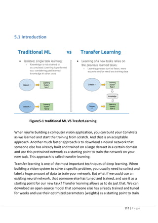
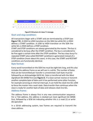
197. 196 | P a g e
8.4.4 connecting raspberry-pi with SSH:
We should make sure that laptop is on the same network as the Raspberry Pi
(the network in the wpa_supplicant.conf file). Next, we want to get the IP
address of the Raspberry Pi on the network. By running arp -a we will see IP
addresses of other devices on the network. This will give a list of devices and
the corresponding IP and MAC addresses. We should see our Raspberry Pi listed
with its IP address.
Then Connecting to the Raspberry Pi by running ssh pi@ [the Pi's IP Address].
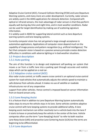
8.5 connection between Arduino and Raspberry-pi:
There are only limited number of GPIO pins available on the Raspberry Pi, so
it would be great to expand the input and output pins by linking Raspberry
Pi with Arduino. In this section we will discuss how we can connect the Pi
with single or multiple Arduino boards. You have three options to connect
them I2C.
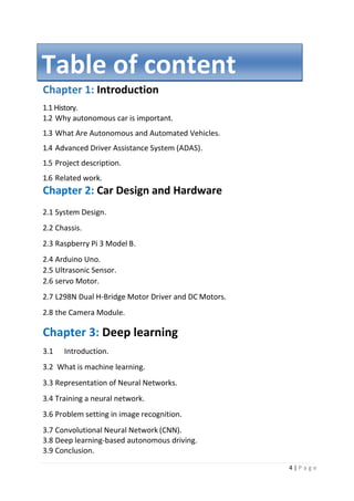
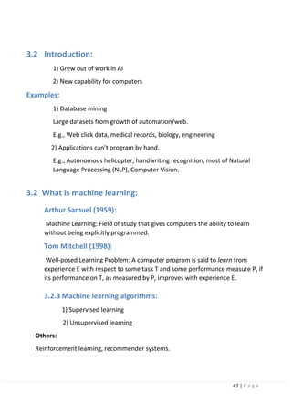
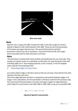
8.5.1 Setup:
Figure 8.8 Hardware schematics

198. 197 | P a g e
first step: Linking the GND of the Raspberry Pi to the GND of the Arduino.
Second step: Connecting the SDA (I2C data) of the Pi (pin 2) to the Arduino SDA.
Third step: Connecting the SCL (I2C clock) of the Pi (pin 3) to the Arduino SCL.
Important note: Raspberry Pi 4 (and earlier) is running under 3.3V, and the
Arduino Uno is running under 5V!
We should really pay attention when we connect 2 pins between those boards.
Usually we’d have to use a level converter between 3.3V and 5V. But in this
specific case we can avoid If the Raspberry Pi is configured as a
master and the Arduino as a slave on the I2C bus, then we can connect the SDA
and SCL pins directly. To make it simple, in this scenario the Raspberry Pi will
impose 3.3V, which is not a problem for the Arduino pins.

199. 198 | P a g e
References:
Chapter 1:
1.The Pathway to Driverless Cars. Claire Perry
2.wordpress.com
3.theguardian.com
Chapter 2:
1.https://www.raspberrypi.org/help/what-%20is-a-raspberry-pi/
2.https://www.arduino.cc/en/guide/introduction
Chapter 3:
1-D. Cheng, Y. Gong, S. Zhou, J. Wang, N. ZhengPerson re- identification by multi-
channel parts-based cnn with improved triplet loss function Proc. of IEEE
Conference on ComputerVision and Pattern Recognition (27-30 June2016),
10.1109/CVPR.2016.149 Google Scholar
2-P. Viola, M. JonesRapid object detection using a boostedcascade of simple features
Proc. of IEEE Conference on Computer Vision and Pattern Recognition (8-14 Dec.
2001), 10.1109/CVPR.2001.990517 Google Scholar
3-N. Dalal, B. TriggsHistograms of oriented gradients forhuman detection Proc. of
IEEE Conference on Computer Vision and Pattern Recognition (20-25 June 2005),
10.1109/CVPR.2005.177 Google Scholar
4-G. Csurka, C. Dance, L. Fan, J. Willamowski, C.BrayVisual categorization with bags of
keypoints Proc. of ECCV Workshop on Statistical Learning in Computer Vision
(2004) Google Scholar
5-D.G. LoweDistinctive image features fromscale-invariant keypoints Int. J. Comput.
Vis., 60 (2004), pp. 91-110 rossRefView Record in Scopus Google Scholar
6-Y. Lecun, L. Bottou, Y. Bengio, P. HaffnerGradient-basedlearning
applied to document recognition Proc. IEEE, 86 (1998), pp. 2278-2324 View
Record in Scopus Google Scholar
7-S. Ren, K. He, R. Girshick, J. Sun“Faster R-CNN: Towards Real- Time Object Detection
with Region Proposal Networks,” inIEEE Transactions on Pattern Analysis and
Machine Intelligence 39 (6) (1 June 2017), pp. 1137-1149,
10.1109/TPAMI.2016.2577031 CrossRefView Record in Scopus Google Scholar
8-J. Redmon, S. Divvala, R. Girshick, A. FarhadiYou only lookonce: unified, real-time
object detection Proc. of IEEE Conference on Computer Vision and Pattern
Recognition (27-30 June 2016), 10.1109/CVPR.2016.91 Google Scholar
9-J. Long, E. Shelhamer, T. DarrellFully convolutional networksfor semantic
segmentation Proc. of IEEE Conference on Computer Vision and Pattern
Recognition (7-12 June 2015), 10.1109/CVPR.2015.7298965 Google Scholar
10-M. Cordts, M. Omran, S. Ramos, T. Rehfeld, M. Enzweiler, R. Bene nson, U. Franke,
S. Roth, B. SchieleThe cityscapes dataset for semantic urban scene understanding
Proc. of IEEE Conference on Computer Vision and Pattern Recognition (27-30 June
2016), 10.1109/CVPR.2016.350 Google Scholar
11-A. Moujahid, M.E. Tantaoui, M.D. Hina, A. Soukane, A. Ortalda, A. ElKhadimi, A.
Ramdane-CherifMachine learning techniques in ADAS: a review Proc. of 2018

200. 199 | P a g e
International Conference on Advances in Computing and Communication
Engineering (22-23 June 2018), 10.1109/ICACCE.2018.8441758 Google Scholar
12- J. Levinson, J. Askeland, J. Becker, J. Dolson, D. Held, S. Kammel, J.Z. Kolter, D.
Langer, O. Pink, V.R. Pratt, M. Sokolsky, G. Stanek, D.M. Stav ens, A. Teichman, M.
Werling, S. ThrunTowards fully autonomous driving: systems and algorithms
Intelligent Vehicles Symposium (2011), pp. 163-168 CrossRefView Record in
ScopusGoogle Scholar
Chapter 4:
1. https://www.dlology.com/blog/how-to-train-an-object-detection-
model-easy-for-free/
2. https://arxiv.org/abs/1806.08342
3. https://machinelearningmastery.com/object-recognition-with-deep-
learning/
4. https://arxiv.org/abs/1512.02325
5. https://arxiv.org/abs/1506.02640
6. https://medium.com/@prvnk10/object-detection-rcnn-
4d9d7ad55067,https://arxiv.org/pdf/1807.05511.pdf
7. https://arxiv.org/abs/1504.08083
8. https://arxiv.org/abs/1506.01497
Chapter 5:
1. Deep Learning for Vision Systems by Mohamed Elgendy
2. https://manalelaidouni.github.io/manalelaidouni.github.io/Evaluatin g-Object-Detection-
Models-Guide-to-Performance-Metrics.html
3. Deep Learning for Vision Systems by Mohamed Elgendy
Chapter 6:
[1] David tian “Deep pi car” [online] available.
https://towardsdatascience.com/deeppicar-part-1- 102e03c83f2c
[2] Mr. Tony Fan, Dr. Gene Yeau-Jian Liao, Prof. Chih-Ping Yeh, Dr. Chung-Tse Michael
Wu, Dr. Jimmy Ching- MingChen “Lane Keeping system by visual technology
“[online] available. https://peer.asee.org/lane-keeping- system- by-visual-
technology.pdf
[3] Prof. Albertengo Guido “Adaptive Lane Keeping Assistance System design based on
driver’sbehavio”. [online] available.
https://webthesis.biblio.polito.it/11978/1/tesi.pdf
[4] David tian ‘’End-to-End Lane Navigation Model via Nvidia Model’’ online
[available].
https://colab.research.google.com/drive/14WzCLYqwjiwuiwap6aXf9imhyctjRMQp

201. 200 | P a g e
Chapter 7:
[1] Carmine Noviello, Mastering STM32A step-by-step guide to themost complete
ARM Cortex-M platform, using a free and powerful development
environment based on Eclipse and GCC.
[2] TCP Connection Establish and Terminate” [online] available.
https://www.vskills.in/certification/tutorial/information-technology/basic- network-
support-professional/tcp-connection-establish-and-terminate/
[3] anonymous007, ashushrma378, abhishek_paul ” Differences between TCP and
UDP” [online] available. https://www.geeksforgeeks.org/differences-between-tcp-
and-udp/