GPUFish is a parallel computing framework for solving very large-scale matrix completion problems on GPUs. It implements parallel stochastic gradient descent to optimize the matrix completion objective function. GPUFish allows customizing the objective function to domain-specific problems like 1-bit matrix completion where entries are binary. Tests show GPUFish achieves a 100x speedup over serial algorithms for 1-bit matrix completion with minimal loss in accuracy using a single GPU.

1. GPUFish: A Parallel Computing Framework for
Matrix Completion from A Few Observations
Charlie Hubbard and Chinmay Hegde
Electrical and Computer Engineering Department
Iowa State University
November 25, 2016
Abstract
The problem of recovering a data matrix from a small sample of observed entries, also known
as matrix completion, arises in several real-world applications including recommender systems,
sensor localization, and system identification. We introduce GPUFish, a parallel computing
software framework for solving very large-scale matrix completion problems. GPUFish is modular,
tunable, inherently parallelizable, and leverages the massive number of multiple concurrent kernel
executions possible on a modern GPU.
The algorithmic core of GPUFish is an optimized implementation of the Jellyfish framework [1]
which employs parallel stochastic gradient descent for solving the matrix completion problem.
GPUFish enables the user to fine-tune the loss function to domain-dependent problems, thus
extending the matrix completion framework to non-numeric observations. As a stylized application,
we demonstrate how to adapt GPUFish to solve the 1-bit matrix completion problem where the
matrix observations are binary [2]. Our results demonstrate that we achieve a 100x speedup over
existing serial algorithms for this problem, with only a minimal loss in prediction accuracy, using
a standard workstation equipped with a single GPU.
1 Introduction
1.1 Motivation
The problem of recovering a data matrix from a small sample of its entries, also called the matrix completion
problem, arises in several real-world applications including content recommender systems, sensor localization,
and system identification.
The matrix completion problem rose to prominence during the Netflix Prize [3]. The problem faced by Netflix
was the following: given a subset of movie ratings provided by users, how best to predict future (unknown)
movie ratings? Put differently, imagine a large ratings matrix M with rows representing users and columns
representing movies. Given a partially observed subset of the entries of M, the goal was to fill in the rest of
the missing (unobserved) entries.
This problem poses three central challenges. First, for a content provider such as Netflix, even the most active
users can only rate a small fraction of the movies available, and therefore the matrix of observed ratings is
extremely sparse. Without additional information, the task of recovering M would seem impossible. However,
the recent, large body of work in matrix completion has shown that as long as the matrix M possess a
sufficiently low rank, we can recover the missing entries of M via a convex optimization procedure [4–7].
1

2. Users/Movies
Han 1 2
Leia 3 2
Luke 3 4
Rey 5 3
Users/Movies
Han 1 4 3 3
Leia 3 3 2 2
Luke 4 3 4 2
Rey 5 2 2 3
GPUFish
Figure 1: In a collaborative filtering environment, one can use GPUFish to predict user-movie ratings and
complete an incomplete ratings matrix.
Second, for large-scale content providers such as Netflix, Amazon, and Spotify, their popularity, and sheer
amount of content available, implies that the number of users and the number of items can both be in the
order of hundreds of millions (as of December 2015, Amazon had over 300 million registered users). Matrices
this large (greater than a few thousand rows/columns) cause problems for typical matrix completion methods,
and convex optimization approaches are not particularly suitable. To resolve this, a non-convex, incremental
heuristic for matrix completion was introduced in [1]. This method, termed as Jellyfish, achieves this
speed-up by using a specific randomized version of incremental gradient descent, which allows data points to
be processed in parallel with no fine-grained memory locking.
Third, the application of standard approaches for matrix completion to the problem of content recommendation
is not seamless. The matrix completion literature assumes that the entries of the matrix are real-valued;
however, the ratings provided by users of content providers are almost always “quantized” to some finite set
of integers (for example, Netflix ratings range from 1 to 5, while Pandora only allows a binary like/dislike
system.) Treating such categorical ratings as if they were quantized versions of a “true” real number creates
a number of issues; for example, if a user’s “true” rating of a particular movie in Netflix is 7.8 but we cap the
reported rating at a maximum of 5, then we have introduced a significant amount of observation noise that
is unaccounted for during the recovery of the remaining ratings. To remedy this, the framework of 1-Bit
matrix completion has been presented in [2] and outperforms contemporary matrix completion methods by
intrinsically modeling the ratings as non-numeric entities. However, the challenge now is to solve an even
more complicated convex optimization procedure, and again the issue of scalability in this setting is further
exacerbated.
1.2 Our contributions
In this technical report, we introduce GPUFish, a parallel computing software framework for solving matrix
completion problems for arbitrary data types. To the best of our knowledge, our proposed framework is the
first to extend and massively parallelize generic matrix completion solution approaches.
2

3. GPUFish is modular, tunable, and leverages the massive number of multiple concurrent kernel executions
possible on a modern GPU. As a stylized application, we demonstrate how to adapt GPUFish to solve the
1-bit matrix completion problem where the matrix observations are binary [2]. Our results demonstrate that
we achieve a 150x speedup over existing serial algorithms, while maintaining comparable prediction accuracy.
Our work demonstrates that a standard workstation equipped with a single GPU can be effectively deployed
to solve very large scale matrix completion problems.
A C++ implementation of GPUFish is available for download at https://github.com/cghubbard/gpu-fish.
1.3 Our techniques
The algorithmic core of GPUFish is an optimized implementation of the Jellyfish framework [1]. Similar
to the approach proposed in [1], our approach also employs a randomized, incremental stochastic gradient
descent; this enables us to work in the factorized space, never having to store the entire ratings matrix in
memory during the training process.
However, GPUFish generalizes the previous approach in two distinct ways: (i) GPUFish enables the user to
transparently adapt to domain-dependent problems, thus extending the matrix completion framework to
numeric as well as non-numeric observations. (ii) GPUFish enables the user to leverage the full parallel
processing power of a GPU, and can concurrently process hundreds of available samples in the training phase;
this considerably accelerates training time over known existing approaches.
2 Application: Scalable Collaborative Filtering
As a stylized application, we describe an instantiation of GPUFish for solving large scale instances of the
matrix completion (also sometimes called collaborative filtering) problem where the user ratings are available
in the form of binary (like/dislike) observations.
2.1 Setup: 1-bit matrix completion
We adopt the 1-bit matrix completion model of [2]. Our goal is to complete any missing entries of a rank-r
matrix M with nr rows and nc columns, given an observed subset of its entries, denoted by Ω ⊆ [nr] × [nc].
Here, the entries of M represent the underlying interest (or “enjoyment”) level that a user i has in item j.
However, in a departure from classical matrix completion, we do not get to directly observe the entries of M.
Instead, consider any twice-differentiable function p : R → [0, 1]. We record observations Y such that:
Yi,j =
+1 with probability p(Mi,j),
−1 with probability 1 − p(Mi,j),
for (i, j) ∈ Ω. (2.1)
In other words, Y is a matrix of identical size as M, where the entry Yi,j is +1 with high probability if
user i “enjoys” item j (i.e., Mi,j is high), and −1 otherwise. As with previous work in matrix completion,
it is important that Ω is chosen uniformly at random; this can be implemented, for example, if any
(i, j) ∈ {1, . . . , nr} × {1, . . . , nc} is independently included in Ω with probability E[|Ω|]
nrnc
.
In [2], the Probit and Logit functions, often employed in model fitting in statistics, are explored as natural
functions to model the underlying distribution of the entries of Y. Suppose we focus on the Logit function
p(x) = ex
1+ex . To recover an estimate of M we can maximize the log-likelihood function of the optimization
variable X over the set of observations Ω. Denote 1A as the indicator function over a Boolean condition A.
Then the log-likelihood function corresponding to the Logit model is given by:
3

4. LΩ,Y(X) :=
(i,j)∈Ω
1Yi,j =1 log(p(Xi,j)) + 1Yi,j =−1 log(1 − p(Xi,j) . (2.2)
The estimate of M, therefore, is given by the solution to the constrained optimization problem1
:
M = argmax
X
LΩ,Y(X),
s.t. rank(X) ≤ r .
(2.3)
2.2 Factorized version of optimization problem
The optimization problem (2.3) is non-convex, due to the presence of the rank constraint on X. The
standard method adopted in matrix completion approaches is to perform a nuclear norm relaxation of the
rank constraint. However, nuclear norm-regularized matrix recovery formulations can incur a high running
time [1,4,6].
In order to resolve this issue, we adopt the Jellyfish approach of [1]. Jellyfish can be used to solve
problems of the form:
minimize
(i,j)∈Ω
fij(Xij) + P(X), (2.4)
where g is any convex loss function of a scalar and P : Rnr×nc
→ R is a matrix regularizer that encourage
low-rank solutions. In our implementation, we use the γ2-norm as a regularizer [8]. The γ2-norm is defined as
the infimum of the matrix maximum-row-norms of the factors of X, measured over all possible factorizations
of X:
X γ2
:= inf max L 2
2,∞, R 2
2,∞ : X = LR∗
, (2.5)
Here, · 2,∞ denotes the maximum row-norm of any matrix, A:
A 2,∞ := maxj
k
A2
jk
1/2
. (2.6)
Assuming that the decision variable X is at most rank-r, we can rewrite it at X = LR∗
, where the size of L and
R are nr × r and nc × r, respectively. Note that explicit storage of X requires memory capacity proportional
to nrnc, which is infeasible for most matrices encountered in large-scale collaborative filtering applications.
Instead, by writing our decision variable as LR∗
, we only incur a memory requirement proportional to
(nr + nc)r, a significant reduction.
We now consider a constrained version of (2.4) (where the regularization term is explicitly bounded by a
parameter B):
minimize
(i,j)∈Ω
fij(Xij) subject to X γ2 ≤ B . (2.7)
The optimal value of B is empirically chosen on a per dataset basis.
We replace f by the negative log-likelihood function specified in 2.3, and also assume the factorized version
of the γ2-norm defined above. With a bit of algebraic simplification, we obtain the bilinear optimization
problem:
1To be precise, the problem formulation in [2] also included a boundedness constraint on M ∞, but we omit that constraint
here.
4

5. minimize
(i,j)∈Ω
−L(LR∗
) subject to L 2
2,∞ ≤ B, R 2
2,∞ ≤ B. (2.8)
To solve (2.8), we adopt the incremental projected gradient descent approach of [1]. We alternately update L
(resp., R) while keeping R (resp., L) fixed. In each iteration, the updates to L and R are given by [1]:
L
(k+1)
ik
= ΠB Lik
− αkL (L
(k)
ik
R
(k)∗
jk
)R
(k)
jk
R
(k+1)
ik
= ΠB Rik
− αkL (L
(k)
ik
R
(k)∗
jk
)L
(k)
jk
(2.9)
where the projection operator Π onto the constraint set in (2.8) admits the closed form expression:
ΠB(v) =
√
Bv
v v 2
≥ B
v otherwise
. (2.10)
Here Li is the ith
row of L and Rj is the jth
row of R so L
(k)
ik
R
(k)∗
jk
is the estimated value of matrix M(i, j).
The step size parameter in the gradient descent iteration, αk, is a positive scalar that decreases by a constant
amount at every iteration.
2.3 Parallelization
The above gradient descent formulation of the matrix recovery has several computational advantages.
Primarily, we observe that the updates performed in (2.9) operate on highly local portions of the matrices
L and R. That is any pair (i, j) ∈ Ω will only read from and write to the rows Li and Rj. Given a pair
of points from Ω, (i1, j1) and (i2, j2) we could perform the gradient updates for these points in parallel as
long as i1 = i2 and j1 = j2; they are entirely unrelated. In the same manner, if we had two sets of points
S1 = {(i, j) : i ∈ I1, j ∈ J1} and S2 = {(i, j) : i ∈ I2, j ∈ J2} with I1 ∩ I2 = ∅ and J1 ∩ J2 = ∅, the gradient
updates for each set could be run, in principle, completely in parallel. This is the intuition exploited in [1];
however, they have focused on standard matrix completion as a special case, and also assume a standard
multi-core computing model.
We first describe the scheme for sample ordering, called cyclic partitioning, developed in depth in [1]. We
introduce some terminology. Any two (row or column) index sets S1 and S2 are said to be overlapping if
either I1 ∩ I2 = ∅ or J1 ∩ J2 = ∅. Therefore, if the observed data points in Ω were suitably partitioned into
non-overlapping groups, then each group could be independently processed.
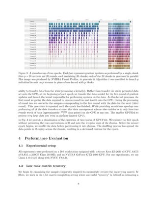
A simple way to group the data is to divide our matrix M into four smaller blocks. An illustration is displayed
in Fig. 2. For consistency with [1] we will refer to these blocks as chunks and index any chunk C as Ca,b
where a and b are row and column indices of the chunk in the partitioned matrix. From Figure (2), it is clear
that the blocks on the diagonal of M, B1,1 and B2,2, are non-overlapping, as are the off-diagonal blocks,
B1,2 and B2,1. It is also clear that any two chunks Ca,b and Ca ,b are overlapping if a = a or b = b .
We know that non-overlapping chunks can be safely processed in parallel; so we will define two rounds of
chunks where R1 = {C1,1, C2,2} and R2 = {C2,1, C1,2}; in this way we are free to process the chunks in each
round in parallel as they are non-overlapping. If we process the rounds sequentially, no two parallel processes
will ever be writing or reading from the same rows of R or L at the same time and we can eschew any locking
delays between the different processes.
Extending our example, we observe that if we have the means to process p chunks in parallel we will need
to divide our matrix into p2
chunks and divide the chunks into p rounds. Before we can determine the
appropriate chunk for the data points (i, j) ∈ Ω we generate random permutations of the row and column
indices of our matrix M, πrow and πcol to ensure that the data points in any chunk differ between subsequent
5

6. L1
L2
R1 R2
L1R1 L1R2
L2R1 L2R2
L R* = M
Figure 2: A chunking of our matrix. Non-overlapping chunks are of the same color and are grouped into
rounds. Here we have 4 chunks in 2 rounds.
passes over that data set. In addition, we use without-replacement sampling to determine the order that
observed samples are placed in chunks. Again, from [1] we place any data point (i, j) ∈ Ω according to the
following shuffling rule:
a =
p
nr
(πrow(i) − 1) + 1 and b =
p
nc
(πcol(j) − 1) + 1. (2.11)
With the entire data set placed into chunks we are ready to perform our parallel gradient updates.
3 GPUFish
3.1 Optimized computation
Thus far, our approach is a straightforward adaptation of Jellyfish for the 1-bit matrix completion problem.
However, in contrast with [1], we will perform our updates on a graphics processing unit (GPU) which, unlike
a traditional CPU, can perform simultaneous computations on different parts of the data.
We provide a high level description of the organization of a GPU. Each process instantiated on the GPU is
known as a kernel. A kernel can be executed in parallel across several threads of the GPU. The programmer
(or compiler) groups the parallel threads into blocks and the blocks into a grid of blocks. When launching a
kernel on the GPU, the user controls the number of blocks to launch as well as the number of threads per
block to launch. Each thread launched by the kernel executes an instance of that kernel. Threads in a block
execute concurrently. The execution of thread blocks is performed by streaming multiprocessors, or SMs for
short. The number of blocks that can be executed in parallel by a single SM depends on the resources used
by each block, the resources available in each SM, and the number of SMs in the GPU.
We leverage this architecture for our incremental gradient descent algorithm. Suppose that we have divided
Ω into p2
chunks. We will launch a single kernel for each of the p rounds we have created. As noted above,
the kernels must be launch sequentially to perform the parallel updates without fine-grained locking. Each
round will contain p chunks so we will instantiate our kernel with p blocks. Each block will be responsible for
performing gradient updates (2.9) for all data points (samples) in the corresponding chunk. Each block of
the kernel will contain r worker threads, where r is the rank of M. Each thread, tk, in a given block will be
6

7. Algorithm 1 GPUFish
Given: a data set Ω
1: Permute rows and columns of M, shuffle Ω
2: Separate Ω into p2
chunks
3: Round[i] = p chunks s.t. all chunks are non-overlapping
4: Transfer data for Round[1] to GPU
5: for i = 1 to p in parallel do
6: Launch GPU Gradient Updates kernel with p blocks and r threads per block
7: Transfer data for Round[i+1] to GPU overwriting the data from Round[i-1]
8: end for
Algorithm 2 GPU Gradient Updates
Given: p chunks
1: for each of p chunks in parallel do
2: for each data point (i, j, rating) in the chunk do
3: apply (2.9) to L and R
4: end for
5: end for
responsible for updating Lik and Rjk, that is the kth
entry in the rows of L and R being updated by 2.9
according to the data point (i, j, Yi,j). In this way, we not only perform the gradient updates for a large
number of data points, but also update in parallel the r entries of any row of L or R. In contrast with [1],
using this procedure we get an r-fold speedup per round.
We can further optimize running time as follows. While a given kernel (corresponding to one of the rounds) is
being processed by the GPU, we simultaneous loading the data required to execute the next kernel onto the
GPU. At the completion of the given we remove its data from the GPU and continue to the next round. The
process of chunking our data and then performing parallel gradient updates over p kernels is known as an
epoch. Because each epoch requires a new shuffle of our dataset, we begin each epoch by launching a separate
CPU thread to compute the shuffle required for the next epoch; this extra CPU thread is executed in parallel
with the GPU kernel launches being handled by the main CPU.
The procedure above is an adaptation of Jellyfish for the GPU, which we will call GPUFish. Algorithm 1
describes the overall action of a single epoch of GPUFish.
3.2 Data management
We discuss some specific schemes for managing the various observations and variables that a practical
implementation of GPUFish would encounter. As mentioned above, to compute our gradient updates (2.9)
we launch p blocks each with r threads; where r is the rank of our matrix. Each block is responsible for the
serial processing of all the points in a single chunk and the threads allocated to each block allow us to load,
update and store in memory the relevant rows L and R in a single step.
Before the first epoch, the matrices L and R are loaded into the global memory of the GPU where they can
be accessed by all threads of the GPU. We initialize L and R with uniformly distributed random entries
from [−0.5, 0.5], we scale these entires by 1
sqrt(nr×nc) . Thread access to global memory is generally slow, so
rather than make repeated calls to global memory we begin by loading the relevant rows of L and R into
shared memory on the GPU. This memory is shared only between the threads of each block and access to it
is significantly faster than global memory. After completing our computation of (2.8) from our copies of L
and R in shared memory we write the our updates to L and R back to global memory.
In addition to making use of the GPU’s faster shared memory, we also make use of the ability of the GPU’s
7

8. Figure 3: A visualization of two epochs. Each bar represents gradient updates as performed by a single chunk.
Here p = 20 so there are 20 rounds, each containing 20 chunks; each of the 20 chunks is processed in parallel.
This image was produced by NVIDIA Visual Profiler, to generate it Algorithm 1 was modified to launch p
individual kernels on p streams in place of one kernel with p blocks.
ability to transfer data from the while processing a kernel(s). Rather than transfer the entire permuted data
set onto the GPU, at the beginning of each epoch we transfer the data needed for the first round of gradient
updates and launch the kernel responsible for performing updates on the data. As this kernel processes the
first round we gather the data required to process round two and load it onto the GPU. During the processing
of round two we overwrite the samples corresponding to the first round with the data for the next (third
round). This procedure is repeated until the epoch has finished. While providing an obvious speedup over
performing all of the data transfers at once, this data management scheme also enables us to only have two
rounds worth of data (approximately 2× Ω
p data points) on the GPU at any one. This enables GPUFish to
process very large data sets even on memory-limited GPUs.
In Fig. 3 we provide a visualization of the execution of two epochs of GPUFish. We execute the first epoch
without permuting the rows and columns of Ω and note the irregular sizes of the chunks. Before the second
epoch begins, we shuffle the data before partitioning it into chunks. The shuffling process has spread the
data points in Ω evenly across the chunks, resulting in a decreased runtime for the epoch.
4 Performance Evaluation
4.1 Experimental setup
All experiments were performed on a Dell workstation equipped with: a 6-core Xeon E5-2620 v3 CPU, 64GB
of RAM, a 256GB Class 30 SSD, and an NVIDIA GeForce GTX 1080 GPU. For our experiments, we use
Linux 3.10.0-327 along with NVCC V8.0.26.
4.2 Low rank matrix recovery
We begin by examining the sample complexity required to successfully recover the underlying matrix M
(Here, we work in the 1-bit matrix completion setting where successful “recovery” is defined as estimating a
8

9. matrix from the signs of a subset of its observations).
We describe the experimental setup. A random nr × nc matrix M was formed such that M = MLM∗
R where
ML is nr × r and MR is nc × r; the entires of ML and MR were independently sampled from a uniform
distribution on [-1
2 , 1
2 ]. Here nr = nc = 4000. Entries of M were drawn at random for both the training
set (the size of which varied) and the test set (1000 entries). The input parameters for our model — the
maximum row sum of M and the gradient step size α — were determined using a grid search. The input
rank to the model was the (known) true rank of M, though overestimating the rank seemed to have little
effect on our results. To measure accuracy of our model we record the percentage of samples in our test
set whose sign is correctly predicted by the sign of f( ˆM) where ˆM is our estimate of M. Figure 1 displays
results for the r = 1 and r = 3 cases.
0 1 2 3 4 5 6 7 8
Number of Samples/(Rank*Dimension)
0.5
0.6
0.7
0.8
0.9
1
PercentTestSamplesRecovered
Samples Recovered vs Number of Samples
Rank =1
Rank = 3
Figure 4: Percentage of test samples recovered as a function of the number of samples input into GPUFish.
Here the number of samples is given as a fraction of the rank of the matrix (r = 1 and r = 3) and the
dimension (d = 4000).
4.3 Collaborative filtering with real data
In our next batch of experiments we test the ability of GPUFish to make predictions in the collaborative
filtering environment on real-world data. Specifically we make predictions about user interest in movies for
the Movielens (100k , 1m and 20m) data set [9]. Where possible we compare our results to those produced
from the code released with [2].
We transform the user-movie ratings from the Movielens data set (integers in [1, 5]) to one-bit observations
by subtracting the average over all ratings (approximately 3.5) from each rating and recording the sign. Our
input parameters, including rank, are again determined by a grid search. Each instance of GPUFish was
terminated after 20 epochs. For each Movielens data set (100k, 1M and 20M) we remove 5,000 ratings for
testing purposes, and train the model with the remaining ratings. In Table 1 we present the percentage of
one-bit ratings correctly recovered by GPUFish as a function of the original rating. We also display the
overall percentage of ratings correctly recovered as well as the runtime of the algorithm.
In Table 2 we present the present the results of GPUFish as run on the Movielens 20M data set. Here users
are allowed to rate movies on a scale from [0.5, 1, 1.5, . . . , 5].
Empirically we were able to determine the number of blocks per kernel (the number of chunks in a round)
that results in the smallest run time. The results are presented in Figure 4.3. For each epoch we perform
two processes in parallel: gradient updates on the GPU and the permuting and chunking Ω; the run time of
each epoch is the max of the time taken by either of these two processes. Examining Figure 4.3 we see that
executing GPUFish with a larger number of blocks per kernel can only decrease our runtime to the extent
9

10. Original Rating 1 2 3 4 5 Overall Runtime(s)
GPUFish: ML 100k 80% 77% 58% 71% 87% 72% 0.30
1-Bit: ML 100k 79% 73% 58% 75% 89% 73% 47
GPUFish: ML 1m 86% 74% 55% 75% 92% 74% 1.1
1-Bit: ML 1m 84% 76% 53% 77% 94% 75% 3130
Table 1: A comparison between 1-bit matrix completion from [2] and the 1-bit matrix completion implemented
in GPUFish. GPUFish produces results on par with the traditional 1-bit approach and is able to do so in a
fraction of the runtime.
Original Rating 0.5 1 1.5 2 2.5 3 3.5 4 4.5 5 Overall
GPUFish: ML 20m 84% 85% 89% 81% 85% 68% 63% 67% 82% 88% 74%
Table 2: The results of GPUFish operating on the almost 20 million entires of the of the Movielens 20m
data set. Runtime: 30 seconds.
0 50 100 150
Blocks per Kernel
0
5
10
15
20
25
Runtime(s)
0 50 100 150
Blocks per Kernel
0
200
400
600
Runtime(s)
Movielens (1m) Movielens (20m)
Figure 5: The runtime of 20 epochs of GPUFish vs the number of blocks per kernel
that it is no longer determined by the execution of gradient updates. At approximately 30 blocks per kernel
our gradient updates can be performed faster than our permutations and chunking and we no longer see a
decrease in runtime.
4.4 Effect of chunking
We now present preliminary results relating to the effect of chunking on the ability of GPUFish to make
accurate predictions. For both the Movielens 1m and 20m data sets GPUFish was run as described in
Algorithm 1 and then run with a modified algorithm where the data was permuted and chunked prior to
epoch one and never again. Recall that chunking for epoch t+1 is performed in parallel with the gradient
updates for epoch t; ideally these steps would take equal amounts of time but, as shown in Table 3, we find
that after the initial permutation of data additional permutations significantly increase the time per epoch of
GPUFish, but have little effect on the accuracy of our predictions.
References
[1] B. Recht and C. R´e. Parallel stochastic gradient algorithms for large-scale matrix completion. Math.
Programming Computation, 5(2):201–226, 2013.
10

11. GPUFish Data set Accuracy Runtime (s) Time per epoch (s)
w/ chunking ML 1m 74% 1.1 0.055
w/o chunking ML 1m 74% 0.48 0.024
w/ chunking ML 20m 74% 30 1.5
w/o chunking ML 20m 74% 6.5 0.33
Table 3: GPUFish run with and without between-round chunking on the Movielens 1m and 20m data sets.
Removing between-round chunking had no effect on accuracy and significantly decreased runtime.
[2] M. Davenport, Y. Plan, E. van den Berg, and M. Wootters. 1-bit matrix completion. Information and
Inference, 3(3):189–223, 2014.
[3] J. Bennett and S. Lanning. The netflix prize. In Proc. KDD Cup and Workshop, 2007.
[4] Emmanuel J Cand`es and Benjamin Recht. Exact matrix completion via convex optimization. Found.
Comput. Math., 9(6):717–772, 2009.
[5] E. Cand`es and T. Tao. The power of convex relaxation: Near-optimal matrix completion. IEEE Trans.
Inform. Theory, 56(5):2053–2080, 2010.
[6] E. Cand`es and Y. Plan. Matrix completion with noise. Proceedings of the IEEE, 98(6):925–936, 2010.
[7] B. Recht. A simpler approach to matrix completion. J. Machine Learning Research, 12(Dec):3413–3430,
2011.
[8] G. Jameson. Summing and nuclear norms in Banach space theory, volume 8. Cambridge University Press,
1987.
[9] F Maxwell Harper and Joseph A Konstan. The movielens datasets: History and context. ACM Transactions
on Interactive Intelligent Systems (TiiS), 5(4):19, 2016.
11