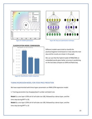
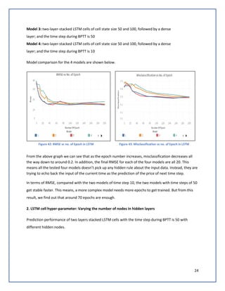
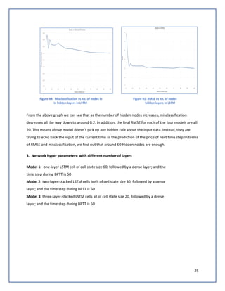
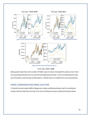
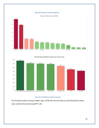
The document discusses predicting Google stock prices using machine learning algorithms. It explores using news sentiment data and historical stock prices to build regression and time series forecasting models. Multiple linear regression, ARIMA, and Holt-Winters exponential smoothing models were tested on the data, with ARIMA producing the best results with an RMSE of 123.73 on test data. The aim is to improve predictive accuracy of Google stock movements.

1. 1
OPIM – 5671 – DATA MINING AND BUSINESS INTELLIGENCE
GOOGLE STOCK PRICE FORECASTING
Project White Paper
August 17, 2018
TEAM DATA SQUAD
Arkaprava Kundu
Rishitha Gajjala
Shanmugha Priya Akhilesshwar
Sanjay Vishwakarma

2. 2
Table of Contents
INTRODUCTION.............................................................................................................................................3
PROBLEM STATMENT....................................................................................................................................3
LITERATURE REVIEW.....................................................................................................................................4
DATA .............................................................................................................................................................4
EXPLORE........................................................................................................................................................6
DATA PRE-PROCESSING ................................................................................................................................8
1. DATA CLEANING ........................................................................................................................................8
2. DATA TRANSFORMATION..........................................................................................................................9
3. DATA PARTITIONING .................................................................................................................................9
MACHINE LEARNING...................................................................................................................................10
MULTIPLE LINEAR REGRESSION..................................................................................................................10
TIME SERIES MODELING .............................................................................................................................10
PROPHET MODEL........................................................................................................................................16
DEEP LEARNING ALGORITHM .....................................................................................................................16
MODEL COMPARISON AND MODEL SELECTION.........................................................................................26
GOOGLE STOCK PRICE FORECASTING FOR JULY 2018 ................................................................................28
LEARNING CURVE FOR THE BEST MODEL...................................................................................................28
BUSINESS INSIGHTS.....................................................................................................................................29
FUTURE WORK............................................................................................................................................30
REFERENCES................................................................................................................................................31

3. 3
INTRODUCTION
Stock price forecasting is a popular and important topic in the field of Finance because of its volatility. It
attracts researchers to capture the unpredictability and predict its next moves. Stock brokers and market
analysts continuously study the pattern of stocks to plan their buy or sell strategies. Internal to Google, it
is important for them to know what triggers the stock price and what downfalls it. This influence various
business decisions taken in Google. Stock market produces huge amount of data every day, so it’s not an
easy task to predict the future stock price considering all the current and past information. There are two
main approaches to predict the stock prices, one being Technical analysis and other being Fundamental
analysis. Technical analysis used the past prices and volume to predict the future trend whereas
Fundamental analysis uses other financial and economic factors which influence the stock prices. In this
paper, we have collected both technical and fundamental data from online sources for Google (Parent
company ALPHABET) to forecast Google stock price. The popularity of Google and availability of heaps of
information online for our research, motivated us to choose Google stock price forecasting.
PROBLEM STATMENT
Our project mainly aims to improve the predictive accuracy of Google stock prices and determine if Time
series forecasting and LSTM models can be used to offer insights regarding the future stock prices and
how other external events and factors are impacting the stock prices. On a broad perspective, we target
to build models to predict the rise and fall of the stock price pattern and forecast the day-to-day stock
price of Google that would help the company for a better planning. Thus, our problem can be categorized
into two: Classification (to predict rise and fall pattern) and Regression (to predict the stock prices).
Our team decided to implement the same using Machine learning, Time series and Deep learning
algorithms. Data sources used and the work corresponding to each of the data sources are mentioned
below.
NEWS HEADLINES
Classification of whether the stock prices will have an upward/downward trend using news headline
data (where previous day’s news is used). Misclassification rate is the estimation metrics used.
HISTORICAL STOCK DATA

4. 4
Stock price prediction based on historical stock data. RMSE is the estimation metrics. Another
estimation metrics is the Misclassification rate (the number of times stock price trend -
upward/downward is correctly predicted on the whole test dataset).
LITERATURE REVIEW
Stock price prediction is based on the implications of Efficient Market Hypothesis (EMH) that stock price
reacts instantaneously to day-to-day news. Work has been done to predict the direction of stock price
index movement using soft computing-based models such as Artificial Neural Networks (ANN) and
Support Vector Machines. Other approaches like Fuzzy Logic, Genetic Algorithm, Machine Learning
algorithms were also implemented. Hidden Markov Models (HMM) approach was used to forecast stock
price for interrelated markets. This approach helped in pattern recognition and classification problems
because of its ability for dynamic system modeling.
Econometric models that include methods such as Autoregressive method (AR), Moving average model
(MA), Autoregressive Moving average (ARMA) model, Autoregressive Integrated moving average
(ARIMA) models have been used for stock prediction and other time series analysis. Researchers have
also experimented to enhance the basic ARIMA model for improved accuracy. These experiments
helped the researchers understand that additional features should be brought into picture apart from
the historical stock data. This resulted in gathering online news related to stock from various public
media and textual information was processed further for news evaluation. One such work includes an
automated text mining approach to gather news data from various sources, analyze using Natural
Language Processing (NLP) techniques to determine the sentiment of news articles and its impact on the
fluctuating energy demands. Work has also been done on Twitter feeds where keyword tagging was
used to understand about the airline's customer satisfaction.
Our approach is to combine the traditional time series analysis with sentiment scores generated from
the text mining process done on New York Times news headlines thereby incorporating additional
features which will help in improving the stock price prediction accuracy.
DATA
Our data of historical stock is sourced from Yahoo Finance and New York Times data is pulled from
official developer site. This data is recorded daily and made publicly available for further analysis.

5. 5
Internal to Google, this data helps them take strategic decisions. External to Google, stock brokers and
market analyst use this information to take buy/sell decisions. Lots of money revolves around this useful
data. We have collected the stock price and New York times data for past 10.5 years -7th
Jan 2008 to
29th
June 2018. Our target variable is opening stock price. The different news sections included were
National, Business, World, U.S. Politics, Opinion, Tech, Science, Health. For web scraping we have used
Newsapi.articles library of python that allows to pull headlines from New York Times using Archive API
from the URL - http://api.nytimes.com/svc/archive/v1/{}/{}.json?api-key={}
Once the web scraping is completed, SentimentIntensityAnalyzer from NLTK API was used to generate
positive, negative, neutral and compound sentiments based on polarity-based and valence-based
approach. Using both approaches helps us not only in classifying a news as positive, negative or neutral
but also takes the intensity of the sentiment into account which is expressed in terms of Compound
sentiment score.
INPUTS AND STATISTICS
The set of predictors includes company finance related predictors, socio – economic predictors and
various events which were captured during this time frame. Sharp rise and falls in the time series were
explored to find events and the duration of those events that had an impact on stock prices.
Events captured
• Stock Market Crash- 2008
• Black Monday -2011
• Apple Impact-2012
• Hurricane Sandy -2012
• Google Internet Growth2013
• Pres- Election -2016
• EU Fine -2017
• Import Tariff -2018, Sep Low,
• Quarterly Impact
Statistics
Open
Prices
Comp
Sentiment
Negative
Sentiment
Neu
Sentiment
Positive
Sentiment
Count 2735 2735 2735 2735 2735
Mean 495.58 -0.79 0.13 0.77 0.09
Std.Dev 270.72 0.52 0.03 0.05 0.02
Min 131 -0.99 0 0 0
25% 275 -0.99 0.11 0.75 0.07
50% 404 -0.99 0.13 0.77 0.09
75% 709 -0.96 0.15 0.8 0.1
Max 1188 0.99 0.27 1 0.23
Table 1: Summary statistics of dataset

6. 6
Feature engineering helped us pull socio economic predictors like Federal Fund Rate, Inflation, Gold, SP
500. Other company related features which we have included are Revenue, Assets and Liabilities. For
each of the event, a dummy variable (new column) has been created and 1s were populated against the
duration of the events. Thus, each of the events contributed to become a variable in our dataset and the
duration of the event that actually influenced the stock price were captured.
EXPLORE
Exploratory Data Analysis (EDA) is the first step in the data analysis process. Statistical graphics is a
collection of techniques--all graphically based and all focusing on one data characterization aspect. We
have incorporated the graphical representations using R, Python and SAS tools.
ANALYSIS OF RAW DATA & ITS DISTRIBUTION
Plots were created to understand the
distribution of each of the variables.
Plot below shows that the variables
Asset, liabilities, Federal Fund rate,
negative Sentiment, stock volume,
open Prices, neutral sentiment and
compound sentiment had skewness
issues and needs to be transformed.
Figure 1: Data distribution

7. 7
CORRELATION
How correlation & multi-collinearity
were handled?
We observed that stock volume and
SP 500 are highly correlated, so we
choose to remove stock volume.
Asset, Liabilities and Revenue seem
to be multicollinear. So, we have
removed these variables.
TIME SERIES DECOMPOSITION
For time series analysis, it is important that the data is stationary. For the data to be stationary, trend and
seasonal components must be removed. We proceeded to decompose the time series using frequency of
100. From the graph below, we can see that there is an upward trend and seasonality in the time series
data.
Figure 3: Time series decomposition
Figure 2: Correlation plot

8. 8
STATIONARITY TESTS
To further confirm the presence of trend and seasonality, Unit root test and seasonal root test were
performed. As per the unit root test of Dickey -Fuller, we observed that series is not stationary. This is
because p value is significantly high, so we reject null hypothesis that series is stationary, which implies
that trend exists.
As per the seasonal root test of Ljung- Box test, we observed that seasonality exists in the time series. This
is because p- value is significantly high, so we reject the null hypothesis that series is stationary, which
also implies that seasonality exists in the series. Having confirmed both trend, trend and seasonlity would
be handled during time series modeling.
Figure 4: Test for stationarity
DATA PRE-PROCESSING
Our dataset went through a series of steps during preprocessing phase. The sub steps under this are
mentioned below in two sections
1. DATA CLEANING
Our data of stock prices is present in frequency of 5 days. Weekday’s stock price is provided, however
the stock prices on holidays was missing. Every year there were around 12 days of missing stock prices.
So, we choose LOCF (Last observation carry forward technique) to impute the missing values. The
previous observation’s stock price is considered on the holiday. This makes our data uniform and useful
for further predictions.

9. 9
2. DATA TRANSFORMATION
Below graph shows the data distribution of each variable. Data looks highly skewed and modeling
wouldn’t be efficient if these variables are used. Transformations are usually applied so that the data
appear to more closely meet the assumptions of a statistical inference procedure that is to be applied, or
to improve the interpretability or appearance of graphs.
We have tried different transformation techniques like log, square root, cube root, auto box- cox. We
further varied lambda value and observed data was looking nearly normalized with auto box-cox
transformation.
Figure 5: Distribution before transformation Figure 6: Distribution after transformation
3. DATA PARTITIONING
We have 10.5 years of data with 2735 rows. Last 1 year of data from 29-June-2017 to 29-June-2018 is
taken as test set (262 rows). We also decided that we would forecast for one month from 30th June
2018 to 29th July 2018.

10. 10
MACHINE LEARNING
MULTIPLE LINEAR REGRESSION
Since multiple linear regression has the ability to capture the trend we began modeling with multiple
linear regression. With all variables included, the model resulted in a very high RSME. So, we decided to
proceed with variable selection. Forward, backward and mixed stepwise algorithms were used to select
significant variables. Inflation, positive
sentiment, negative sentiment,
compound sentiment, gold, Federal fund
rate, Net income, Gross profit margin,
SP500_open and events like Black
Monday, Presidential election, EU Fine,
import tariff, Sept low were also selected
as significant variables. Interactions were
also added and the resulting model ended
up in a RMSE of 120. Above graph is plotted for Actual open prices(blue) versus predicted stock
prices(red) for test data. Though the model was able to capture the increasing trend, the predicted
values showed vast variances when compared to the actual values.
TIME SERIES MODELING
Figure 8: Time series plot
Time series was implemented to do the forecasting process. We first proceeded with decomposing the
time series to find trend, seasonality and then worked to make the data stationary after which
Figure 7: Actual(blue) vs predicted(red) stock price using
Linear regression

11. 11
different time series models like Holt winters, Exponential Smoothing, ARIMA models were
implemented. We also incorporated the sentiment scores and other regressors, and finally added
different events identified for improving the model accuracy.
AUTO CORRELATION
The ACF plots show significant autocorrelation is present in the data.
From ACF plot, we can see that the time
series of open prices is not random, but
rather has a high degree of autocorrelation
between adjacent values.
DIFFERENCING
To make the data stationary, we proceeded with
first differencing of the data. On first differencing
we see that the series plot appears to be stationar
y. On doing the dickey fuller test, the null hypothe
sis is less than 0.01, which means that the series is
stationary.
The ACF plot below shows the absence of any significant autocorrelation in the first difference. The
PACF plot shows random significant lags.
Figure 11: ACF plot after first difference Figure 12: PACF plot after first difference
Figure 9: ACF plot on time series data
Figure 10: After First difference

12. 12
SEASONAL DIFFERENCING
We proceeded with seasonal differencing using a frequency of 365, since we have daily data for 10.5
years. On plotting the series, and doing a Dickey Fuller test, the series proves to be stationary. The ACF
plot shows slow decay of the autocorrelation function suggests the data follow a long-memory process.
A higher order autoregressive term in the data. The PACF plot shows a significant lag till 4
The series plot shows that it is s
tationary, and doing a Dickey F
uller test the p value is 0.01, wh
ich means that we can reject th
e null hypothesis and say that
the series is stationary.
Figure 14: Seasonal difference ACF plot Figure 15: Seasonal difference PACF plot
Once the differencing is applied, we proceeded with time series modeling.
HOLT WINTERS MODEL
Winters is a way to model three aspects of the time series: an average value, trend and seasonality. This
method uses exponential smoothing to encode lots of values from the past and predict typical values for
the future. Initially we used the Holt-winters exponential and holt winters trend models, but they did
not perform well on the test data, giving very high RMSE. Since there is presence of both trend and
seasonality in the data, we proceeded with the Holts seasonal model.
Figure 13: Series with seasonal difference

13. 13
HOLTS SEASONAL MODEL Hol
t-Winters seasonal uses an exponential smoothing with trend and additive seasonal component.
The additive model is used when the seasonal variation remains constant through time.
The model resulted with a hig
h alpha value and the gamma value as 1, which shows that the data highly depends on recent trend and
seasonality. Applying the Holts seasonal model on the test data, we get a very high RMSE of 292.4075.
We see that the Holtwinters seasonal model is not fitting the test data well. Hence, we proceeded with
ARIMA.
ARIMA
Advantages of ARIMA model is that it takes into consideration previous values in the time series (AR
terms) and the errors made by previous predictions (MA terms). This allows the model to rapidly adjust
for sudden changes in trend, resulting in more accurate forecasts. Since the first difference data was
stationary, we did an ARIMA model using first difference and on using auto.arima, it selected the same
ARIMA model as the best model, i.e., ARIMA(0,1,0) . The ACF and PACF plots from figure 11 and figure
12 shows that there is no significant autocorrelation in the data. The model gave an RMSE of 123.73 on
the test data
sigma^2 estimated as 6.031e-05: log likelihood=8508.43
AIC=-17014.87 AICc=-17014.86 BIC=-17009.05
RMSE: 123.73
Table 3: Results of ARIMA(0,1,0)
ARIMA SEASONAL
Since there is seasonality present in the data, we tried ARIMA seasonal models. Taking a frequency of
365, we checked the ACF and PACF plots. The PACF plots indicate an AR model of P value 4. However,
trying to implement a seasonal P value of 4, the model fitting failed for a frequency of 365 with seasonal
SMOOTHING PARAMETERS
alpha: 0.7212766
beta: 0
gamma: 1
RMSE: 292.4075
Table 2: Results from Holts
seasonal modelFigure 16: Actual(blue) vs predicted(red) stock price on test data using Holts Seasonal

14. 14
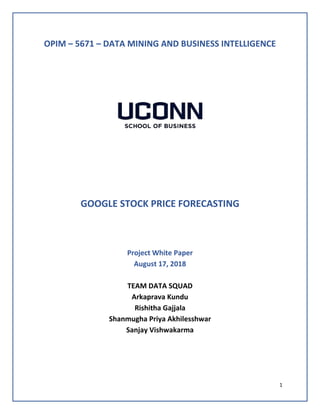
differencing. Hence, we applied an auto ARIMA with seasonal difference of 1, and the best model that
came was ARIMA(1,1,1)(0,1,0). The auto ARIMA function returns the best ARIMA model according to
either AIC, AICC or BIC value. The function conducts a search over all possible models within the order
constraints provided. The RMSE on the test set is 65.755. Best time series model that resulted in lowest
RMSE is ARIMA(1,1,1)(0,1,0).
sigma^2 estimated as 0.0001042: log likelihood=6674.37
AIC=-13342.75 AICc=-13342.74 BIC=-13325.79
RMSE: 65.75556
Table 4: Model Results for ARIMA(1,1,1)(0,1,0)[365]
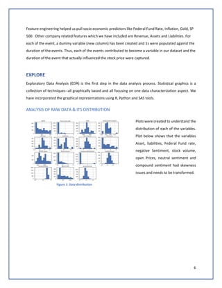
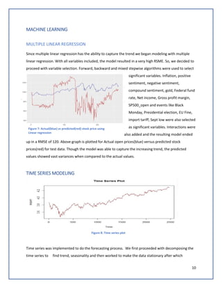
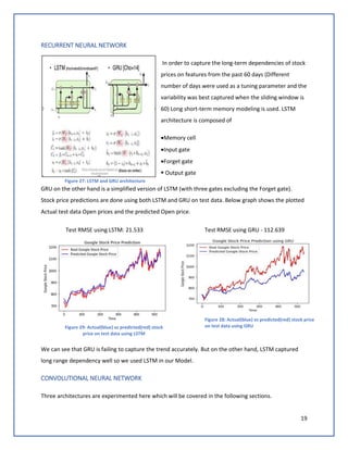
The plot shows th
e difference betw
een actual and pre
dicted open prices
for test dataset.
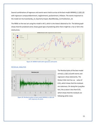
ARIMA WITH REGRESSORS
We then added all regressors (Compound Sentiment, Negative Sentiment, Neutral Sentiment, Positive
Sentiment, Gold, Federal Fund rate, Inflation, Net Income, Gross profit margin, Stock Volume,
SP500_open) on the best model ARIMA (1,1,1)(0,1,0).We observed that the RMSE is increasing to 78.98.
This shows that all the regressors might not be significant for the model.
Proceeded to remove insignificant
regressors, and tried adding certain
events, we found that the model RMSE
decreased to 62.7. This shows that
events greatly influence the stock
prediction.
Figure 17: Actual(blue) vs predicted(red) stock price on test data using ARIMA (1,1,1)(0,1,0)
Figure 18: ARIMA with regressors

15. 15
Several combinations of regressor and events were tried to arrive at the best model ARIMA(1,1,1)(0,1,0)
with regressors compoundSentiment, negSentiment, posSentiment, Inflation. The events important to
the model are HurricaneSandy_12, Quarterly Impact, BlackMonday_11,PresElection_16.
The RMSE on the test set using this model is 44.5, which is the lowest obtained so far. The below graph
shows that the predicted series shows good signs of predicting when there might be a rise or fall in the
stock prices.
RESIDUAL ANALYSIS
The Residual plots of the best model
arima(1,1,1)(0,1,0) with events and
regressors show stationarity. The
Dickey Fuller test has a p value of
0.01, which shows that the residuals
are stationary. On doing the Ljung Box
test, the p value is less than 0.01,
which shows that the residuals are
following white noise.
Figure 19: ARIMA model with regressors and events
Figure 20: Residual analysis of best model ARIMA(1,1,1)(0,1,0)
with regressors & events

16. 16
PROPHET MODEL
We also implemented the Prophet model (a forecasting tool by Facebook) using R. This model uses a
Bayesian based curve fitting method to forecast the time series data. It is advantageous as it doesn’t
require much prior knowledge or experience of forecasting time series data since it automatically finds
seasonal trends in data and provides easily understandable parameters.
The plot of the model is shown below. The forecasted confidence interval was plotted and the forecast
clearly shows an increasing trend. However, when we check the RMSE on test data using the mean
(yhat) value, the RMSE is 87.06718, which shows that this model is not predicting well for exact data
(single point data). This suggests that Prophet model is good for forecasting confidence intervals, but
might not be well suited for predicting exact data.
Figure 21: Actual(blue) vs predicted(red) stock price on test data using PROPHET
Best model from ARIMA shows that Positive, Negative, Compound Sentiments and Inflation variables ar
e significant for stock price prediction. Events like Hurricane Sandy, Quarterly Impact, Black Monday, Pre
sidential election helps in improving the accuracy of the model.
DEEP LEARNING ALGORITHM
FEATURE EXTRACTION FROM NEWS HEADLINES FOR DEEP LEARNING
SP500_open, Net Income, Gold, Federal fund rate, Gross profit margin, Inflation, StockMarketCrash_08,
posSentiment, negSentiment, compoundSentiment are the variables used for Deep learning algorithms.

17. 17
Headlines from “Business & Technology” section of New York Times is extracted resulting in 600 words
for each day stock prediction.
WORD EMBEDDING DICTIONARY
A dictionary is then created for the words extracted and features for each of the words is created to
generate embedded matrix using GloVe vector introduced by Stanford.
Figure 23: Embedded matrix
Since each word has 300 features associated to it, a single day headlines which has 600 words results in
600*300 = 1,80,000 features. Since the number of features is more, CNN algorithm is used for feature
reduction. This data feature is primarily used for the classification part of the problem statement for
identifying the rise and fall for today, next day and day after tomorrow from which the misclassification
rate can be calculated.
MODEL ARCHITECTURE OF HYBRID RNN & CNN MODEL
CLASSIFICATION to detect rise/fall pattern prediction using 2D data for 1 day
Figure 24: Classification model architecture
Figure 22: Data set with features from news headlines

18. 18
News headlines is preprocessed and passed to Convolutional neural network. During pre-processing
vector representation of these words (Word Embeddings) are calculated. Each word has various features
associated to it. Thus, our input to neural network will be an Embedded matrix representation of words
(600 words * 300 features each). Convolution layers are applied on Embedded matrix. They are a set of
filters that have their weights updated as and when the algorithm learns and have a smaller dimension
than the input matrix. Thus, when they slide over the height and width of the input vector, a dot product
is calculated resulting in dimension reduction. Max Pooling is a part of Convolution where layers are
introduced between successive convolution layers helping to reduce the parameters to controlling
overfitting. Output from Max pool layer is then passed on to LSTM cell that has 3 hyper parameters to
set– Activation function, recurrent activation and number of units identified using cross validation. For
the predicted probability to be in the range of 0 to 1, sigmoid function is used.
REGRESSION for stock price prediction using 1D data on sliding window
Data vector is created by
shifting the stock price for 60
days back. We use the 60 days
stock price to predict next day
stock price. We tried by shifting
for different number of days
(30, 60 and 90), but we got better result on 60 days sliding window and proceeded with that. Below
table shows the data vector that has 60 features generated from the past 60 days. Then it is normalized
and passed to the RNN LSTM cells and for the predicted stock price to be zero or positive number, Relu
activation function is used.
Figure 26: 60 features from past 60 days stock price
Figure 25: Regression model architecture

19. 19
RECURRENT NEURAL NETWORK
In order to capture the long-term dependencies of stock
prices on features from the past 60 days (Different
number of days were used as a tuning parameter and the
variability was best captured when the sliding window is
60) Long short-term memory modeling is used. LSTM
architecture is composed of
•Memory cell
•Input gate
•Forget gate
▪ Output gate
GRU on the other hand is a simplified version of LSTM (with three gates excluding the Forget gate).
Stock price predictions are done using both LSTM and GRU on test data. Below graph shows the plotted
Actual test data Open prices and the predicted Open price.
Test RMSE using LSTM: 21.533 Test RMSE using GRU - 112.639
We can see that GRU is failing to capture the trend accurately. But on the other hand, LSTM captured
long range dependency well so we used LSTM in our Model.
CONVOLUTIONAL NEURAL NETWORK
Three architectures are experimented here which will be covered in the following sections.
Figure 27: LSTM and GRU architecture
Figure 29: Actual(blue) vs predicted(red) stock
price on test data using LSTM
Figure 28: Actual(blue) vs predicted(red) stock price
on test data using GRU

20. 20
1. LeNet ARCHITECTURE
Figure 30: LeNet architecture
DIMENSION REDUCTION IN CNN
Word embedded matrix is passed
through LeNet5 architecture for
dimension reduction. A filter with
reduced dimension is applied on data
matrix with stride 1 or 2, and a dot
product is calculated. The resulting
matrix will have reduced dimension.
2. RESIDUAL NETWORK ARCHITECTURE
Residual network architecture is used where-in the weight of a node will also depend on the weight of
the previous node.
Figure 32: Residual network architecture
Figure 31: Dimension reduction in CNN

21. 21
PLAIN NEURAL
With increased number of layers, Plain neural is expected to
overfit reducing the training error. But in reality, the training
error starts to increase after some layer because of exploding
gradient or vanishing gradient. To fix this problem we update
the previous weight to the later part of layer, this way it helps
to retain the information learned by the previous nodes in the
algorithm.
RESIDUAL NETWORK
We can see that the training error is reducing in case of
Residual network and is behaving as expected.
3. INCEPTION MODEL ARCHITECTURE
As shown in the picture below, different dimensional filters are used in this model for capturing the
variation in the data. As the name “Inception” suggests, number of mini models using different
dimensional filters are built within a bigger model.
The diagram shows the
Inception operation on a single
layer where multiple filters have
used to fetch different
information from the different
part of the dataset. This helps to
retrieve features better than the
other network because of the multiple
filters like 5*5, 3*3, 1*1, max pooling, average pooling and so on. Below is the complete Inception
network for all layers where we perform similar operation throughout the network.
Figure 33: Layers vs training error in Plain
Neural
Figure 34: Layers vs training error in Residual
network
Figure 35: Inception model architecture (single layer)

22. 22
Model comparison
Graph shows the model comparison between the three
architectures.
We can see that Inception Network captures better
information the other CNN architectures and gives
highest accuracy.
OPTIMIZATION TECHNIQUE
Adam optimization algorithm is the combination of RMS Prop and Momentum. It does the exponential
smoothing of gradient in both horizontal and vertical direction in order to avoid divergence which helps
to converge gradient descent to global minimum very fast.
Drop out is used to avoid overfitting. It randomly selects nodes to drop in each layer with a given
probability in every cycle of iteration. This forces algorithm to distributes the weight evenly on all the
nodes of network which cause to reduce overfitting. It also has L2 regularization effect.
Figure 36:Figure 35: Inception model architecture (entire network)
Figure 37: Model comparison betweenFigure 38: Model comparison between 3 CNN
architecture

23. 23
Figure 39: ADAM optimization Figure 40: Drop out optimization technique
CLASSIFICATION MODEL COMPARISON
Different models were tried to classify the
positive/negative trend based on news data the next
day and the results are shown in the graph.
We can see that the hybrid model of RNN/CNN on
embedded words gives better accuracy in predicting
on the test data compare to SVM and Naïve bay.
TUNING REGRESSION MODEL FOR STOCK PRICE PREDICTION
We have experimented with three hyper-parameters on RNN LSTM regression model.
1. Training parameters by changing Epoch number and batch size.
Model 1: a one layer LSTM cell of cell state size 100, followed by a dense layer; and the
time step during BPTT is 50.
Model 2: a one layer LSTM cell of cell state size 100, followed by a dense layer; and the
time step during BPTT is 10
Figure 41: Classification model comparison

24. 24
Model 3: two-layer-stacked LSTM cells of cell state size 50 and 100, followed by a dense
layer; and the time step during BPTT is 50
Model 4: two-layer-stacked LSTM cells of cell state size 50 and 100, followed by a dense
layer; and the time step during BPTT is 10
Model comparison for the 4 models are shown below.
Figure 42: RMSE vc no. of Epoch in LSTM Figure 43: Misclassification vs no. of Epoch in LSTM
From the above graph we can see that as the epoch number increases, misclassification decreases all
the way down to around 0.2. In addition, the final RMSE for each of the four models are all 20. This
means all the tested four models doesn’t pick up any hidden rule about the input data. Instead, they are
trying to echo back the input of the current time as the prediction of the price of next time step.
In terms of RMSE, compared with the two models of time step 10, the two models with time steps of 50
get stable faster. This means, a more complex model needs more epochs to get trained. But from this
result, we find out that around 70 epochs are enough.
2. LSTM cell hyper-parameter: Varying the number of nodes in hidden layers
Prediction performance of two layers stacked LSTM cells with the time step during BPTT is 50 with
different hidden nodes.

25. 25
Figure 44: Misclassification vs no. of nodes in Figure 45: RMSE vs no. of nodes
in hidden layers in LSTM hidden layers in LSTM
From the above graph we can see that as the number of hidden nodes increases, misclassification
decreases all the way down to around 0.2. In addition, the final RMSE for each of the four models are all
20. This means above model doesn’t pick up any hidden rule about the input data. Instead, they are
trying to echo back the input of the current time as the prediction of the price of next time step.In terms
of RMSE and misclassification, we find out that around 60 hidden nodes are enough.
3. Network hyper parameters: with different number of layers
Model 1: one-layer LSTM cell of cell state size 60, followed by a dense layer; and the
time step during BPTT is 50
Model 2: two-layer-stacked LSTM cells both of cell state size 30, followed by a dense
layer; and the time step during BPTT is 50
Model 3: three-layer-stacked LSTM cells all of cell state size 20, followed by a dense
layer; and the time step during BPTT is 50

26. 26
One layer - RMSE 17.97 Two layer -RMSE 16.2
Figure 46: One-layered LSTM performance Figure 47: Two-layered LSTM performance
Figure 48: Three-layered LSTM performance
Three layer- RMSE 14.87
Above graph shows that as the number of hidden layers increases, the algorithm captures more trend
and seasonality (left plot) and rise and fall trend (right plot) precisely. In terms of predicting the stock
price fluctuations and next day rise/fall pattern, 3 hidden layers are sufficient for accurate prediction.
MODEL COMPARISON AND MODEL SELECTION
To identify the best model, RMSE of Regression models and Misclassification rate for classification
models tried from Machine Learning, Time series and Deep learning are plotted and shown below.

27. 27
Figure 49: Regression model comparison
Figure 50: Classification model comparison
Our final best model is having 3 hidden -layer, LSTM cells all of cell state size 20, followed by a dense
layer; and the time step during BPTT is 50.

28. 28
GOOGLE STOCK PRICE FORECASTING FOR JULY 2018
With the selected model, we have forecasted the stock price for July 2018 month (our data set is
available only until June 2018). As per our prediction, the stock price in July shows an upward trend and
the price hits $1200. This forecast also matches with last month (July 2018) Google’s stock price which
was around $1200 showing the accuracy of our model.
LEARNING CURVE FOR THE BEST MODEL
Figure 52: Learning curve for Regression model Figure 53: Learning curve for classification model
For the learning curve, we have trained our best model on different sizes of training sets starting
from 100, 250, 400, 600, 800, 1000, 1200, and 1450. We can see that model which is trained on
lower training size has lowest RMSE and Misclassification rate, whereas the same model
performs worst on test data set because as we trained on less data our model is not generalizing
well when we are testing on new data set. As we are increasing the training set size, training
Figure 51: Google stock price forecasted for July 2018

29. 29
errors are increasing and it start performing better on test data set. Finally, the model is trained
on highest size of training set, have almost similar error on test dataset which proves that our best
model is working as expected.
BUSINESS INSIGHTS
• From the table, we can see that when we use the news headlines to do the rise/ fall pattern
classification on same day, the accuracy is lesser compared to predicting next day stock price
and next-to-next day stock
price. This shows that news
headlines have more impact
on next day stock price
compared to today’s stock price and 2 days later stock price.
• Google and stock investors will be able to identify rise and fall pattern of its stock prices for
better planning.
• Past 60 days of stock prices helps in accurate prediction of next day stock price.
• Every Quarter end, Google can expect a fall in stock price.
• Impact of Business & Technology headlines is more on the next day stock price.
CHALLENGES FACED
To retrieve every day’s news headlines from NY Times from multiple huge Json files ranging from 20mb
to 100mb. We wrote an algorithm to scan all files of a folder and parse the Json document and retrieve
the texts from headlines for each day of last 10 and half years using Python from various sections. The
Google Stock price data had missing data for holidays and weekends. So, we choose LOCF (Last
observation carry forward technique) to impute the missing values Stock price data and other features
included were skewed implying that data was not normally distributed. Used Auto Box-cox
transformations on the data to get an approximate normal distribution. During model Selection, based
on different cost functions, different models were available. Final model was selected considering
different metrics.
Figure 54: Business insights from news data

30. 30
FUTURE WORK
• Using sliding window on news headlines, i.e., work with 3D data matrix for improved accuracy.
Lack of infrastructure limited this implementation for the project.
• Increase the size of historical stock price data used.
• RNN Model - Using all feature engineered variables to do predictions on sliding windows.

31. 31
APPENDIX 1 - REFERENCES
https://nlp.stanford.edu/projects/glove/
https://arxiv.org/pdf/1409.4842.pdf
https://adeshpande3.github.io/The-9-Deep-Learning-Papers-You-Need-To-Know-About.html
https://ai.google/research/pubs/pub43022
https://arxiv.org/abs/1512.03385
https://www.sciencedirect.com/science/article/pii/S0022169418303184
https://www.researchgate.net/publication/13853244_Long_Short-term_Memory

32. 32
APPENDIX 2 – FIGURES
Figure 1: Data distribution............................................................................................................................6
Figure 2: Correlation plot..............................................................................................................................7
Figure 3: Time series decomposition............................................................................................................7
Figure 4: Test for stationarity........................................................................................................................8
Figure 5: Distribution before transformation Figure 6: Distribution after transformation......................9
Figure 7: Actual(blue) vs predicted(red) stock price using Linear regression..............10
Figure 8: Time series plot............................................................................................................................10
Figure 9: ACF plot on time series data........................................................................................................11
Figure 10: After First difference..................................................................................................................11
Figure 11: ACF plot after first difference Figure 12: PACF plot after first difference .............................11
Figure 13: Series with seasonal difference .................................................................................................12
Figure 14: Seasonal difference ACF plot Figure 15: Seasonal difference PACF plot.......12
Figure 16: Actual(blue) vs predicted(red) stock price on test data using Holts Seasonal ..........................13
Figure 17: Actual(blue) vs predicted(red) stock price on test data using ARIMA (1,1,1)(0,1,0).................14
Figure 18: ARIMA with regressors ..............................................................................................................14
Figure 19: ARIMA model with regressors and events.................................................................................15
Figure 20: Residual analysis of best model ARIMA(1,1,1)(0,1,0) with regressors & events ..................15
Figure 21: Actual(blue) vs predicted(red) stock price on test data using PROPHET...................................16
Figure 22: Data set with features from news headlines.............................................................................17
Figure 23: Embedded matrix.......................................................................................................................17
Figure 24: Classification model architecture ..............................................................................................17
Figure 25: Regression model architecture..................................................................................................18
Figure 26: 60 features from past 60 days stock price.................................................................................18
Figure 27: LSTM and GRU architecture.......................................................................................................19
Figure 28: Actual(blue) vs predicted(red) stock price on test data using GRU...........................................19
Figure 29: Actual(blue) vs predicted(red) stock price on test data using LSTM .........................................19
Figure 30: LeNet architecture .....................................................................................................................20
Figure 31: Dimension reduction in CNN .....................................................................................................20
Figure 32: Residual network architecture...................................................................................................20
Figure 33: Layers vs training error in Plain Neural......................................................................................21
Figure 34: Layers vs training error in Residual network .............................................................................21
Figure 35: Inception model architecture (single layer)...............................................................................21
Figure 36:Figure 35: Inception model architecture (entire network).........................................................22
Figure 37: Model comparison between......................................................................................................22
Figure 38: Model comparison between 3 CNN architecture......................................................................22
Figure 39: ADAM optimization Figure 40: Drop out optimization technique ....................................23
Figure 41: Classification model comparison ...............................................................................................23
Figure 42: RMSE vc no. of Epoch in LSTM Figure 43: Misclassification vs no. of Epoch in LSTM ...........24
Figure 44: Misclassification vs no. of nodes in Figure 45: RMSE vs no. of nodes...........................25
Figure 46: One-layered LSTM performance Figure 47: Two-layered LSTM performance.....................26

33. 33
Figure 48: Three-layered LSTM performance.............................................................................................26
Figure 49: Regression model comparison...................................................................................................27
Figure 50: Classification model comparison ...............................................................................................27
Figure 51: Google stock price forecasted for July 2018..............................................................................28
Figure 52: Learning curve for Regression model Figure 53: Learning curve for classification model ....28
Figure 54: Business insights from news data..............................................................................................29

34. 34
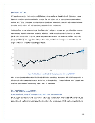
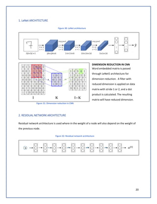
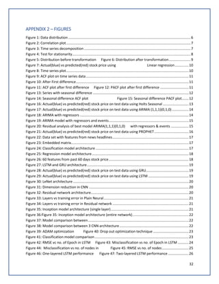
APPENDIX 3 – TABLES
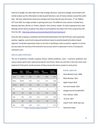
Table 1: Summary statistics of dataset.........................................................................................................5
Table 2: Results from Holts.........................................................................................................................13
Table 3: Results of ARIMA(0,1,0) ................................................................................................................13
Table 4: Model Results for ARIMA(1,1,1)(0,1,0)[365].................................................................................14