Downloaded 21 times
![2 Reinforcement Learning of Policy Networks
The second stage of the training pipeline aims at improving the policy network by policy gradient
reinforcement learning (RL) 25,26
. The RL policy network pρ is identical in structure to the SL
policy network, and its weights ρ are initialised to the same values, ρ = σ. We play games
between the current policy network pρ and a randomly selected previous iteration of the policy
network. Randomising from a pool of opponents stabilises training by preventing overfitting to the
current policy. We use a reward function r(s) that is zero for all non-terminal time-steps t < T.
The outcome zt = ±r(sT ) is the terminal reward at the end of the game from the perspective of the
current player at time-step t: +1 for winning and −1 for losing. Weights are then updated at each
time-step t by stochastic gradient ascent in the direction that maximizes expected outcome 25
,
∆ρ ∝
∂log pρ(at|st)
∂ρ
zt . (2)
We evaluated the performance of the RL policy network in game play, sampling each move
at ∼ pρ(·|st) from its output probability distribution over actions. When played head-to-head,
the RL policy network won more than 80% of games against the SL policy network. We also
tested against the strongest open-source Go program, Pachi 14
, a sophisticated Monte-Carlo search
program, ranked at 2 amateur dan on KGS, that executes 100,000 simulations per move. Using no
search at all, the RL policy network won 85% of games against Pachi. In comparison, the previous
state-of-the-art, based only on supervised learning of convolutional networks, won 11% of games
against Pachi 23
and 12% against a slightly weaker program Fuego 24
.
3 Reinforcement Learning of Value Networks
The final stage of the training pipeline focuses on position evaluation, estimating a value function
vp
(s) that predicts the outcome from position s of games played by using policy p for both players
27–29
,
vp
(s) = E [zt | st = s, at...T ∼ p] . (3)
6](https://image.slidesharecdn.com/deepmindmasteringgoresearchpaper-160129102338/75/Google-Deepmind-Mastering-Go-Research-Paper-6-2048.jpg)
![Methods
Problem setting Many games of perfect information, such as chess, checkers, othello, backgam-
mon and Go, may be defined as alternating Markov games 38
. In these games, there is a state
space S (where state includes an indication of the current player to play); an action space A(s)
defining the legal actions in any given state s ∈ S; a state transition function f(s, a, ξ) defining
the successor state after selecting action a in state s and random input ξ (e.g. dice); and finally a
reward function ri
(s) describing the reward received by player i in state s. We restrict our atten-
tion to two-player zero sum games, r1
(s) = −r2
(s) = r(s), with deterministic state transitions,
f(s, a, ξ) = f(s, a), and zero rewards except at a terminal time-step T. The outcome of the game
zt = ±r(sT ) is the terminal reward at the end of the game from the perspective of the current
player at time-step t. A policy p(a|s) is a probability distribution over legal actions a ∈ A(s).
A value function is the expected outcome if all actions for both players are selected according to
policy p, that is, vp
(s) = E [zt | st = s, at...T ∼ p]. Zero sum games have a unique optimal value
function v∗
(s) that determines the outcome from state s following perfect play by both players,
v∗
(s) =
zT if s = sT ,
max
a
− v∗
(f(s, a)) otherwise.
Prior work The optimal value function can be computed recursively by minimax (or equivalently
negamax) search 39
. Most games are too large for exhaustive minimax tree search; instead, the
game is truncated by using an approximate value function v(s) ≈ v∗
(s) in place of terminal re-
wards. Depth-first minimax search with α − β pruning 39
has achieved super-human performance
in chess 4
, checkers 5
and othello 6
, but it has not been effective in Go 7
.
Reinforcement learning can learn to approximate the optimal value function directly from
games of self-play 38
. The majority of prior work has focused on a linear combination vθ(s) =
φ(s)·θ of features φ(s) with weights θ. Weights were trained using temporal-difference learning 40
in chess 41,42
, checkers 43,44
and Go 29
; or using linear regression in othello 6
and Scrabble 9
.
Temporal-difference learning has also been used to train a neural network to approximate the
optimal value function, achieving super-human performance in backgammon 45
; and achieving
19](https://image.slidesharecdn.com/deepmindmasteringgoresearchpaper-160129102338/75/Google-Deepmind-Mastering-Go-Research-Paper-19-2048.jpg)
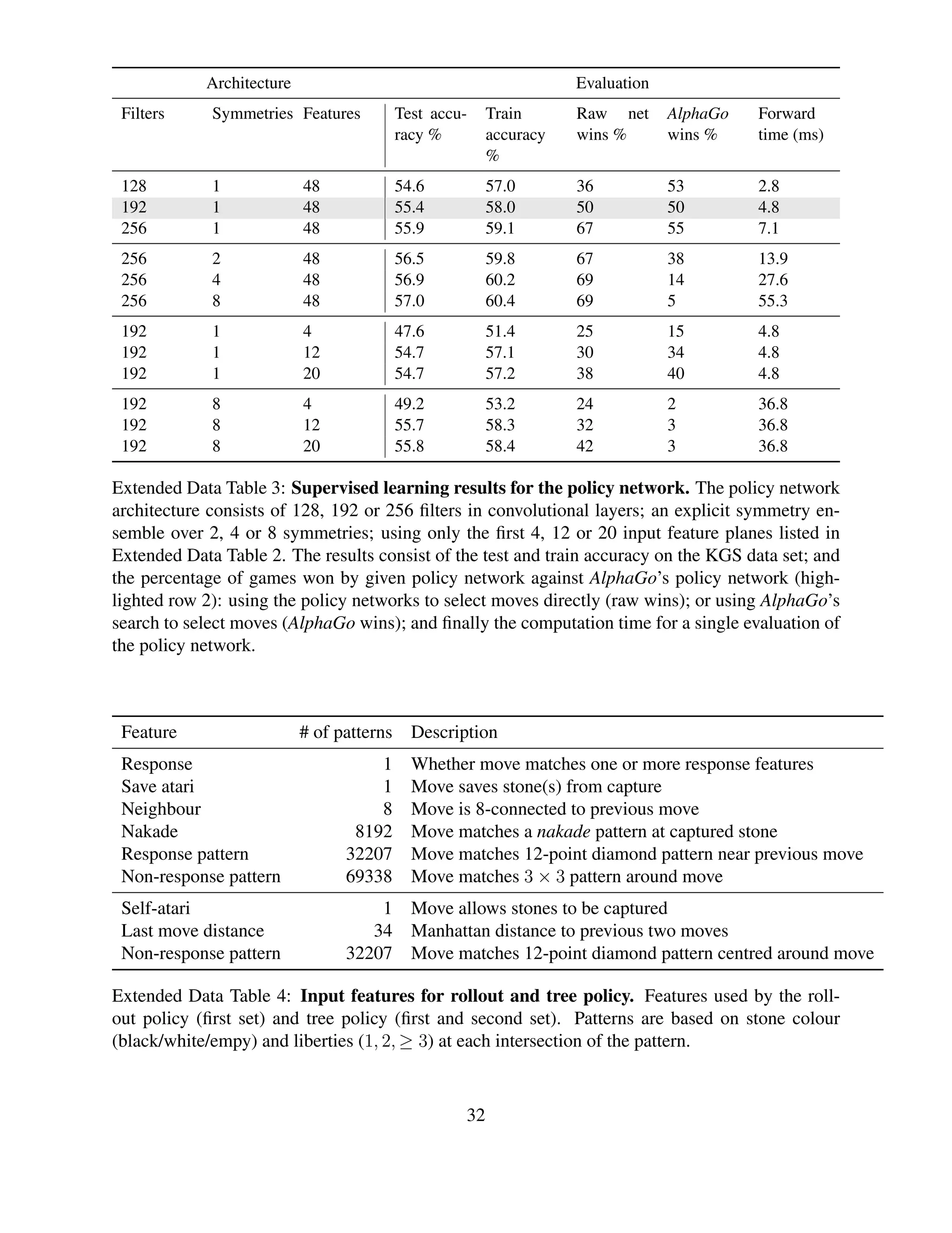
![handcrafted local features encode common-sense Go rules (see Extended Data Table 4). Similar
to the policy network, the weights π of the rollout policy are trained from 8 million positions from
human games on the Tygem server to maximize log likelihood by stochastic gradient descent. Roll-
outs execute at approximately 1,000 simulations per second per CPU thread on an empty board.
Our rollout policy pπ(a|s) contains less handcrafted knowledge than state-of-the-art Go pro-
grams 13
. Instead, we exploit the higher quality action selection within MCTS, which is informed
both by the search tree and the policy network. We introduce a new technique that caches all moves
from the search tree and then plays similar moves during rollouts; a generalisation of the last good
reply heuristic 52
. At every step of the tree traversal, the most probable action is inserted into a
hash table, along with the 3 × 3 pattern context (colour, liberty and stone counts) around both the
previous move and the current move. At each step of the rollout, the pattern context is matched
against the hash table; if a match is found then the stored move is played with high probability.
Symmetries In previous work, the symmetries of Go have been exploited by using rotationally and
reflectionally invariant filters in the convolutional layers 24,27,28
. Although this may be effective in
small neural networks, it actually hurts performance in larger networks, as it prevents the inter-
mediate filters from identifying specific asymmetric patterns 23
. Instead, we exploit symmetries
at run-time by dynamically transforming each position s using the dihedral group of 8 reflections
and rotations, d1(s), ..., d8(s). In an explicit symmetry ensemble, a mini-batch of all 8 positions is
passed into the policy network or value network and computed in parallel. For the value network,
the output values are simply averaged, ¯vθ(s) = 1
8
8
j=1 vθ(dj(s)). For the policy network, the
planes of output probabilities are rotated/reflected back into the original orientation, and averaged
together to provide an ensemble prediction, ¯pσ(·|s) = 1
8
8
j=1 d−1
j (pσ(·|dj(s))); this approach was
used in our raw network evaluation (see Extended Data Table 3). Instead, APV-MCTS makes use
of an implicit symmetry ensemble that randomly selects a single rotation/reflection j ∈ [1, 8] for
each evaluation. We compute exactly one evaluation for that orientation only; in each simulation
we compute the value of leaf node sL by vθ(dj(sL)), and allow the search procedure to average
over these evaluations. Similarly, we compute the policy network for a single, randomly selected
24](https://image.slidesharecdn.com/deepmindmasteringgoresearchpaper-160129102338/75/Google-Deepmind-Mastering-Go-Research-Paper-24-2048.jpg)
![games, using 50 GPUs, for one day.
Value Network: Regression We trained a value network vθ(s) ≈ vpρ
(s) to approximate the value
function of the RL policy network pρ. To avoid overfitting to the strongly correlated positions
within games, we constructed a new data-set of uncorrelated self-play positions. This data-set
consisted of over 30 million positions, each drawn from a unique game of self-play. Each game
was generated in three phases by randomly sampling a time-step U ∼ unif{1, 450}, and sampling
the first t = 1, ..., U −1 moves from the SL policy network, at ∼ pσ(·|st); then sampling one move
uniformly at random from available moves, aU ∼ unif{1, 361} (repeatedly until aU is legal); then
sampling the remaining sequence of moves until the game terminates, t = U + 1, ..., T, from
the RL policy network, at ∼ pρ(·|st). Finally, the game is scored to determine the outcome zt =
±r(sT ). Only a single training example (sU+1, zU+1) is added to the data-set from each game. This
data provides unbiased samples of the value function vpρ
(sU+1) = E [zU+1 | sU+1, aU+1,...,T ∼ pρ].
During the first two phases of generation we sample from noisier distributions so as to increase the
diversity of the data-set. The training method was identical to SL policy network training, except
that the parameter update was based on mean squared error between the predicted values and the
observed rewards, ∆θ = α
m
m
k=1 zk
− vθ(sk
) ∂vθ(sk)
∂θ
. The value network was trained for 50
million mini-batches of 32 positions, using 50 GPUs, for one week.
Features for Policy / Value Network Each position s was preprocessed into a set of 19 × 19
feature planes. The features that we use come directly from the raw representation of the game
rules, indicating the status of each intersection of the Go board: stone colour, liberties (adjacent
empty points of stone’s chain), captures, legality, turns since stone was played, and (for the value
network only) the current colour to play. In addition, we use one simple tactical feature that
computes the outcome of a ladder search 7
. All features were computed relative to the current
colour to play; for example, the stone colour at each intersection was represented as either player
or opponent rather than black or white. Each integer is split into K different 19 × 19 planes of
binary values (one-hot encoding). For example, separate binary feature planes are used to represent
whether an intersection has 1 liberty, 2 liberties, ..., ≥ 8 liberties. The full set of feature planes are
26](https://image.slidesharecdn.com/deepmindmasteringgoresearchpaper-160129102338/75/Google-Deepmind-Mastering-Go-Research-Paper-26-2048.jpg)
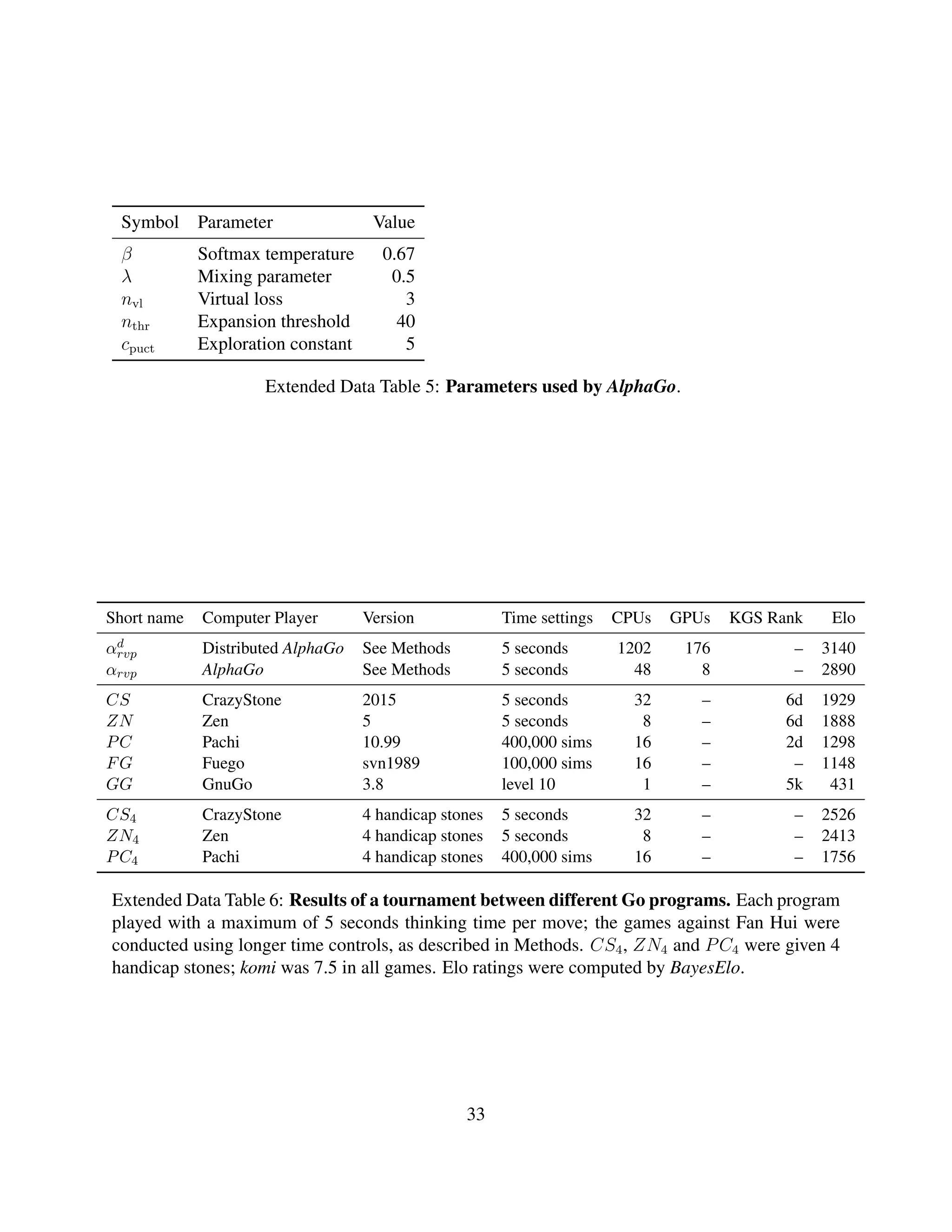
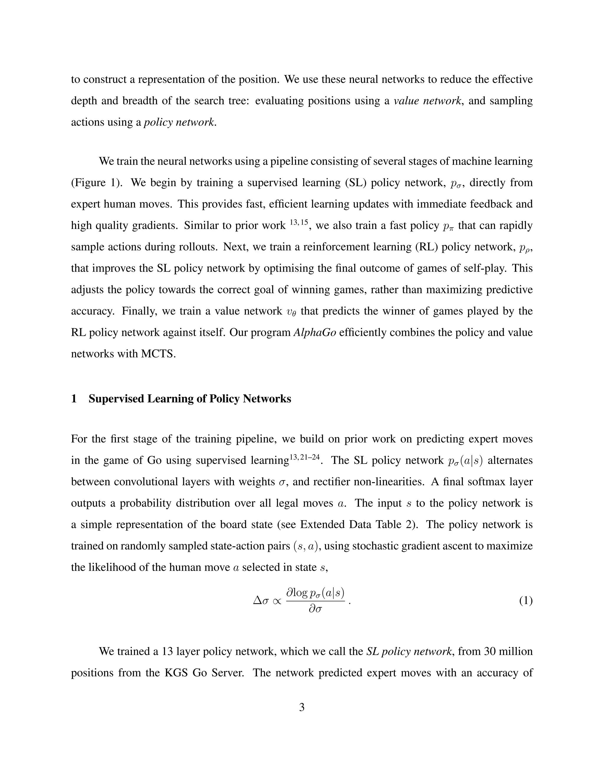
![Short Policy Value Rollouts Mixing Policy Value Elo
name network network constant GPUs GPUs rating
αrvp pσ vθ pπ λ = 0.5 2 6 2890
αvp pσ vθ – λ = 0 2 6 2177
αrp pσ – pπ λ = 1 8 0 2416
αrv [pτ ] vθ pπ λ = 0.5 0 8 2077
αv [pτ ] vθ – λ = 0 0 8 1655
αr [pτ ] – pπ λ = 1 0 0 1457
αp pσ – – – 0 0 1517
Extended Data Table 7: Results of a tournament between different variants of AlphaGo. Eval-
uating positions using rollouts only (αrp, αr), value nets only (αvp, αv), or mixing both (αrvp, αrv);
either using the policy network pσ (αrvp, αvp, αrp), or no policy network (αrvp, αvp, αrp), i.e. in-
stead using the placeholder probabilities from the tree policy pτ throughout. Each program used 5
seconds per move on a single machine with 48 CPUs and 8 GPUs. Elo ratings were computed by
BayesElo.
AlphaGo Search threads CPUs GPUs Elo
Asynchronous 1 48 8 2203
Asynchronous 2 48 8 2393
Asynchronous 4 48 8 2564
Asynchronous 8 48 8 2665
Asynchronous 16 48 8 2778
Asynchronous 32 48 8 2867
Asynchronous 40 48 8 2890
Asynchronous 40 48 1 2181
Asynchronous 40 48 2 2738
Asynchronous 40 48 4 2850
Distributed 12 428 64 2937
Distributed 24 764 112 3079
Distributed 40 1202 176 3140
Distributed 64 1920 280 3168
Extended Data Table 8: Results of a tournament between AlphaGo and distributed AlphaGo,
testing scalability with hardware. Each program played with a maximum of 2 seconds compu-
tation time per move. Elo ratings were computed by BayesElo.
34](https://image.slidesharecdn.com/deepmindmasteringgoresearchpaper-160129102338/75/Google-Deepmind-Mastering-Go-Research-Paper-34-2048.jpg)
![αrvp αvp αrp αrv αr αv αp
αrvp - 1 [0; 5] 5 [4; 7] 0 [0; 4] 0 [0; 8] 0 [0; 19] 0 [0; 19]
αvp 99 [95; 100] - 61 [52; 69] 35 [25; 48] 6 [1; 27] 0 [0; 22] 1 [0; 6]
αrp 95 [93; 96] 39 [31; 48] - 13 [7; 23] 0 [0; 9] 0 [0; 22] 4 [1; 21]
αrv 100 [96; 100] 65 [52; 75] 87 [77; 93] - 0 [0; 18] 29 [8; 64] 48 [33; 65]
αr 100 [92; 100] 94 [73; 99] 100 [91; 100] 100 [82; 100] - 78 [45; 94] 78 [71; 84]
αv 100 [81; 100] 100 [78; 100] 100 [78; 100] 71 [36; 92] 22 [6; 55] - 30 [16; 48]
αp 100 [81; 100] 99 [94; 100] 96 [79; 99] 52 [35; 67] 22 [16; 29] 70 [52; 84] -
CS 100 [97; 100] 74 [66; 81] 98 [94; 99] 80 [70; 87] 5 [3; 7] 36 [16; 61] 8 [5; 14]
ZN 99 [93; 100] 84 [67; 93] 98 [93; 99] 92 [67; 99] 6 [2; 19] 40 [12; 77] 100 [65; 100]
PC 100 [98; 100] 99 [95; 100] 100 [98; 100] 98 [89; 100] 78 [73; 81] 87 [68; 95] 55 [47; 62]
FG 100 [97; 100] 99 [93; 100] 100 [96; 100] 100 [91; 100] 78 [73; 83] 100 [65; 100] 65 [55; 73]
GG 100 [44; 100] 100 [34; 100] 100 [68; 100] 100 [57; 100] 99 [97; 100] 67 [21; 94] 99 [95; 100]
CS4 77 [69; 84] 12 [8; 18] 53 [44; 61] 15 [8; 24] 0 [0; 3] 0 [0; 30] 0 [0; 8]
ZN4 86 [77; 92] 25 [16; 38] 67 [56; 76] 14 [7; 27] 0 [0; 12] 0 [0; 43] -
PC4 99 [97; 100] 82 [75; 88] 98 [95; 99] 89 [79; 95] 32 [26; 39] 13 [3; 36] 35 [25; 46]
Extended Data Table 9: Cross-table of percentage win rates between programs. 95% Agresti-
Coull confidence intervals in grey. Each program played with a maximum of 5 seconds computa-
tion time per move. CN4, ZN4 and PC4 were given 4 handicap stones; komi was 7.5 in all games.
Distributed AlphaGo scored 77% [70; 82] against αrvp and 100% against all other programs (no
handicap games were played).
35](https://image.slidesharecdn.com/deepmindmasteringgoresearchpaper-160129102338/75/Google-Deepmind-Mastering-Go-Research-Paper-35-2048.jpg)
![Threads 1 2 4 8 16 32 40 40 40 40
GPU 8 8 8 8 8 8 8 4 2 1
1 8 - 70 [61;78] 90 [84;94] 94 [83;98] 86 [72;94] 98 [91;100] 98 [92;99] 100 [76;100] 96 [91;98] 38 [25;52]
2 8 30 [22;39] - 72 [61;81] 81 [71;88] 86 [76;93] 92 [83;97] 93 [86;96] 83 [69;91] 84 [75;90] 26 [17;38]
4 8 10 [6;16] 28 [19;39] - 62 [53;70] 71 [61;80] 82 [71;89] 84 [74;90] 81 [69;89] 78 [63;88] 18 [10;28]
8 8 6 [2;17] 19 [12;29] 38 [30;47] - 61 [51;71] 65 [51;76] 73 [62;82] 74 [59;85] 64 [55;73] 12 [3;34]
16 8 14 [6;28] 14 [7;24] 29 [20;39] 39 [29;49] - 52 [41;63] 61 [50;71] 52 [41;64] 41 [32;51] 5 [1;25]
32 8 2 [0;9] 8 [3;17] 18 [11;29] 35 [24;49] 48 [37;59] - 52 [42;63] 44 [32;57] 26 [17;36] 0 [0;30]
40 8 2 [1;8] 7 [4;14] 16 [10;26] 27 [18;38] 39 [29;50] 48 [37;58] - 43 [30;56] 41 [26;58] 4 [1;18]
40 4 0 [0;24] 17 [9;31] 19 [11;31] 26 [15;41] 48 [36;59] 56 [43;68] 57 [44;70] - 29 [18;41] 2 [0;11]
40 2 4 [2;9] 16 [10;25] 22 [12;37] 36 [27;45] 59 [49;68] 74 [64;83] 59 [42;74] 71 [59;82] - 5 [1;17]
40 1 62 [48;75] 74 [62;83] 82 [72;90] 88 [66;97] 95 [75;99] 100 [70;100] 96 [82;99] 98 [89;100] 95 [83;99] -
Extended Data Table 10: Cross-table of percentage win rates between programs in the single-
machine scalability study. 95% Agresti-Coull confidence intervals in grey. Each program played
with 2 seconds per move; komi was 7.5 in all games.
36](https://image.slidesharecdn.com/deepmindmasteringgoresearchpaper-160129102338/75/Google-Deepmind-Mastering-Go-Research-Paper-36-2048.jpg)
![Threads 40 12 24 40 64
GPU 8 64 112 176 280
CPU 48 428 764 1202 1920
40 8 48 - 52 [43; 61] 68 [59; 76] 77 [70; 82] 81 [65; 91]
12 64 428 48 [39; 57] - 64 [54; 73] 62 [41; 79] 83 [55; 95]
24 112 764 32 [24; 41] 36 [27; 46] - 36 [20; 57] 60 [51; 69]
40 176 1202 23 [18; 30] 38 [21; 59] 64 [43; 80] - 53 [39; 67]
64 280 1920 19 [9; 35] 17 [5; 45] 40 [31; 49] 47 [33; 61] -
Extended Data Table 11: Cross-table of percentage win rates between programs in the dis-
tributed scalability study. 95% Agresti-Coull confidence intervals in grey. Each program played
with 2 seconds per move; komi was 7.5 in all games.
37](https://image.slidesharecdn.com/deepmindmasteringgoresearchpaper-160129102338/75/Google-Deepmind-Mastering-Go-Research-Paper-37-2048.jpg)

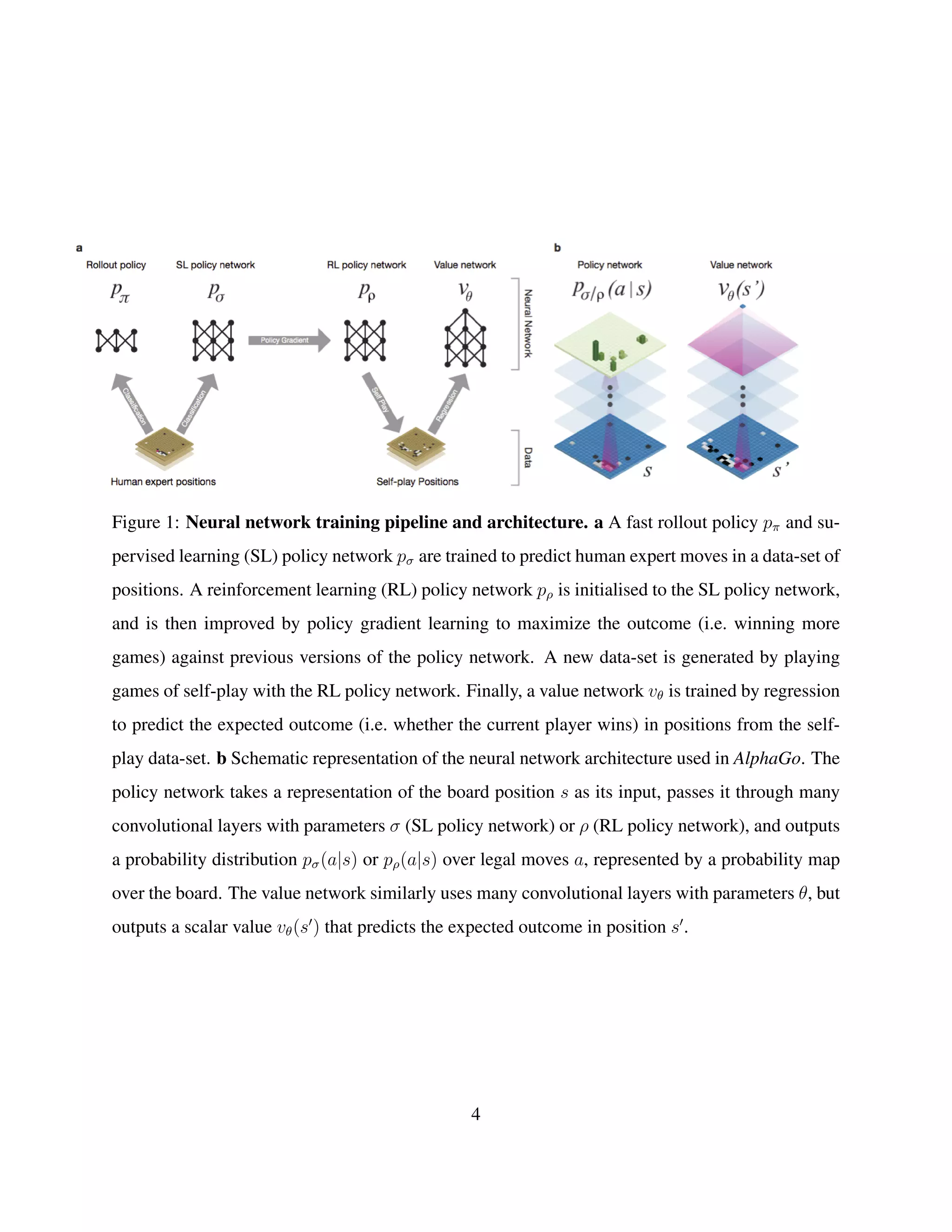
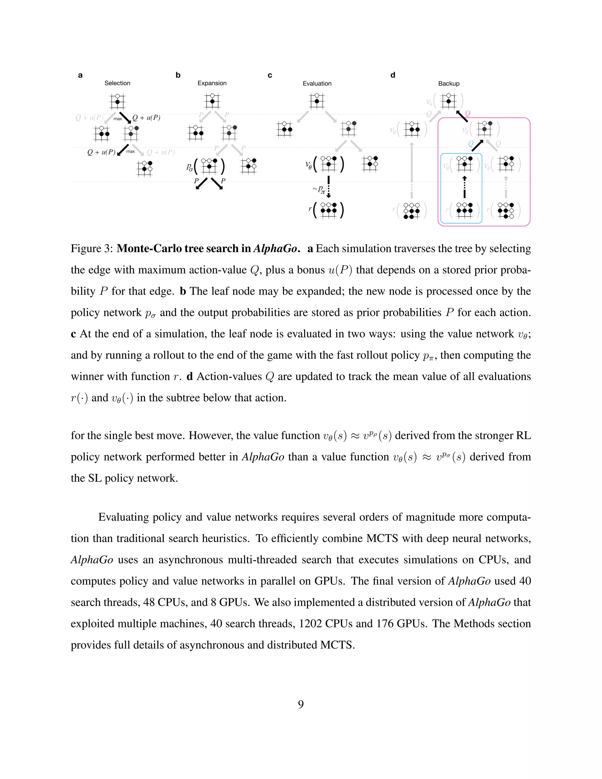
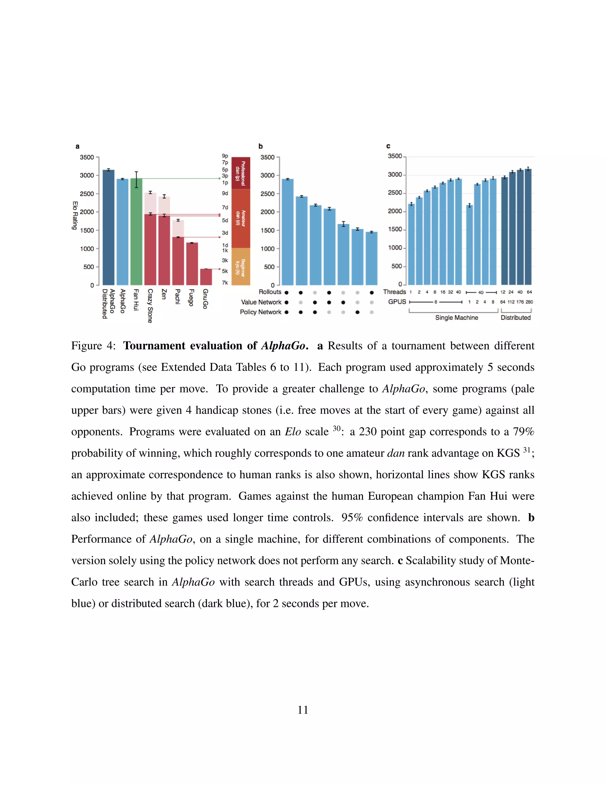
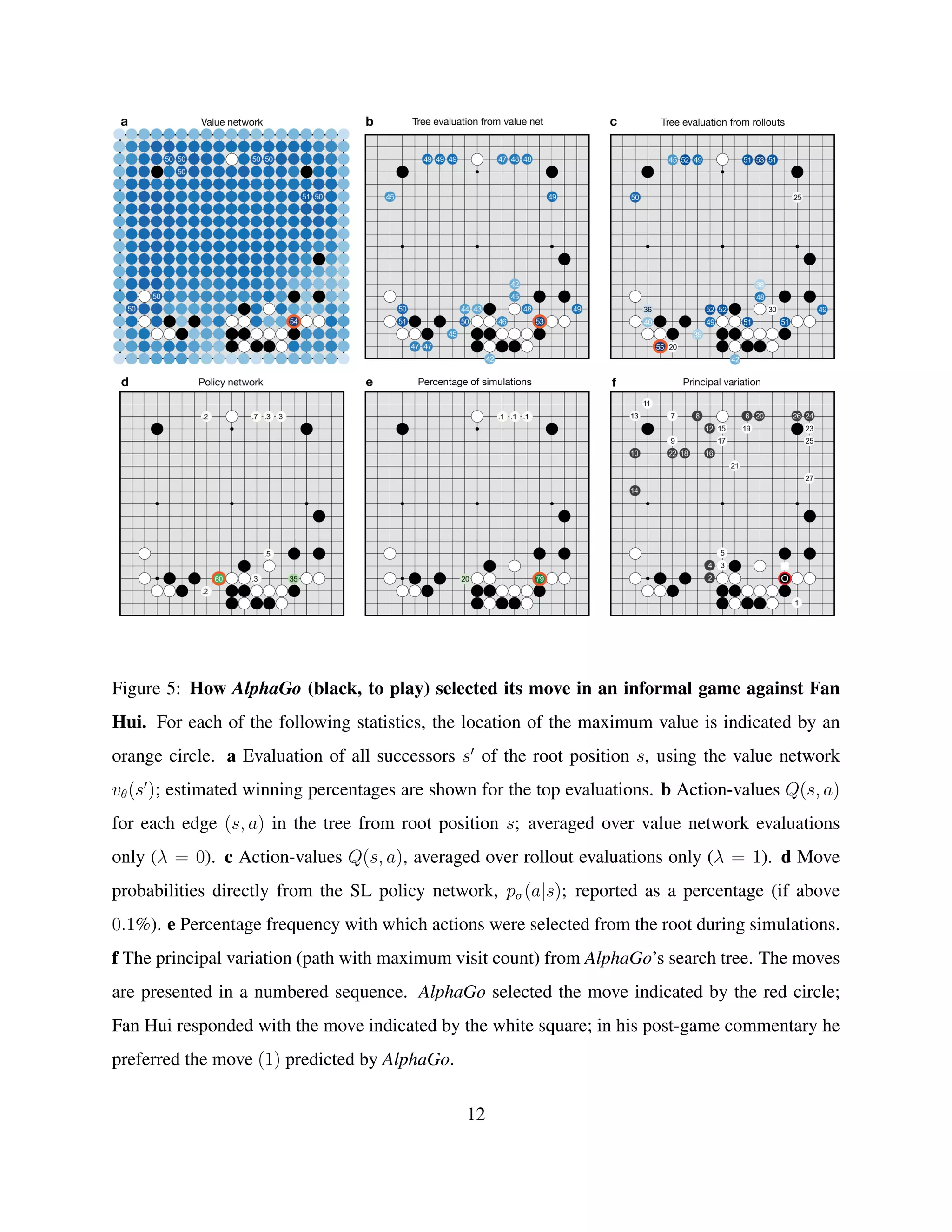
This document summarizes research on developing an AI system called AlphaGo that can defeat human professionals at the game of Go. Key points: 1. AlphaGo uses deep neural networks including a policy network to select moves and a value network to evaluate board positions, trained through both supervised learning from expert games and reinforcement learning from self-play games. 2. Without lookahead search, the neural networks can play Go at a strong amateur level. Combined with a new Monte Carlo tree search algorithm, AlphaGo defeats other Go programs and the European Go champion. 3. This is the first time a computer program has defeated a human professional in the full game of Go, a feat previously thought to be at least