Estimating Static Field Distributions
•
0 likes•121 views

This document discusses techniques for estimating static electric and magnetic fields. It provides examples of point charge fields around lightning rods, power lines, and integrated circuits. It then summarizes the equations that relate electric field strength to charge, geometry, and distance. The document also covers approaches for solving for static fields given boundary conditions or charge/current distributions. These include separation of variables, superposition integrals, and the Biot-Savart law. Finally, it discusses solving for fields in inhomogeneous materials with non-uniform conductivity or permittivity.

Recommended
More Related Content
What's hot
What's hot (20)
Viewers also liked
Viewers also liked (14)
Similar to Estimating Static Field Distributions
Similar to Estimating Static Field Distributions (20)
Recently uploaded
Recently uploaded (20)
Estimating Static Field Distributions
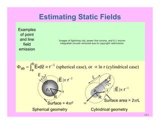
- 1. Estimating Static Fields Examples of point and line Images of lightning rod, power line corona, and 0.1 micron field integrated circuits removed due to copyright restrictions. emission Φ = b E dz − ab ∫a i ∝r 1 (spherical case), or ∝ ln r (cylindrical case) E | |∝ 2 L E E r− ρο r ρο r | |E r∝ −1 R R Surface area = 2πrL Surface = 4πr2 ∞ Spherical geometry Cylindrical geometry L7-1
- 2. L7-2 2 2 2 2 4 ˆ 4 ( ) ( ) = 4 4 • πε = = π ε ⇒ = = πε πε ⇑ ∫ a a r rA V a V aQ Q D n da r E r E r r r r 2 1 1 ( ) 4 4 4 4 ⎛ ⎞ = = = − − ≅ ⇒ = πε⎜ ⎟ πε πε πε⎝ ⎠ ∫ ∫ b b a r aa a Q dr Q Q V E r dr Q V a b a ar (b >> a) a b Simple Static Example Spherical breakdown Q V Lightning rod: a ≅ 1 mm, V 104 volts ⇒ 107 V/m breakdown/corona Power line: a ≅ 1 cm, V 105 volts ⇒ 107 V/m breakdown/corona Integrated Circuit: a ≅ 0.1μm, V = 1 volt ⇒ 107 V/m breakdown/corona > > ( ) = ⇑ a r V E a a ( ) 4 = πε Q V r r ⇓
- 3. L7-3 SOLVING FOR STATIC FIELDS Approaches when given Φ, Ψ on boundaries: q q p V pq Use dv, E4 r ρ Φ = = −∇Φ πε∫ q q p pq 2V pq ˆE r dv 4 r ρ = πε ∫ q p q p q2V p q J (r - r ) H dv 4 | r - r | × = π ∫ Approaches when given ρ, J: z y x dVq rpq Vq rq rp p Superposition integrals Biot-Savart Law Use Laplace’s Equation. Derivation: 2B Electric : ×E = = 0 (statics) E = Φ. ρ = 0 E = 0 Φ = 0 t ∂ ∇ ⇒ ∇ ⇒ ∇ ⇒ ∇ ∂ i . 2D Magnetic : ×H = = 0 (statics; J = 0) H = H = 0 = 0 t ∂ ∇ ⇒ ∇Ψ ∇ ⇒ ∇ Ψ ∂ i
- 4. SEPARATION OF VARIABLES Static charge-free regions obey Laplace’s equation: Electric potential ∇2 Φ(r) = 0 ; Magnetic potential ∇2 Ψ(r) = 0 Assume Φ(x,y) = X(x)Y(y) ⇒ 2 2 2 2 2 ∂ Φ ∂ Φ d X d Y ∇ Φ = + = Y(y) + X(x) = 0 ∂x2 ∂y2 dx2 dy2 2 2 1 d X = − 1 d Y = −k2 "separation constant" X dx2 Y dy2 Solutions: 2 d X 2 = −k X ⇒ X(x) = Acos(kx) + Bsin(kx) dx2 For k2 > 0;2 (swap x,y d Y 2 = + Dsinh(ky)= k Y ⇒ Y(y) Ccosh(ky) dy2 If k2 < 0) or: Y(y) = C'eky + D'e-ky (equivalent to above) L7-4
- 5. SEPARATION OF VARIABLES Solution to Laplace’s equation when k2 = 0: Φ(x,y) = X(x)Y(y) ⇒ Φ(x,y) = (Ax + B)(Cy + D) Example, Cartesian coordinates: {Φ = (Ax+B)(Cy+D) = 0 at x=0 for all y} ⇒ B = 0 Given Φ(x,y) Φo Φ=0 Φ(x,y) 0 y xLx 2 2 0 X dx Y dy = − = Ly 2 2 1 d X 1 d Y 2 2 2 dx 2 d X 0= X(x) = Ax + B d Y 0 Y(y) = Cy + D⇒ dy ⇒ = {Φ = (Ax+B)(Cy+D) = 0 at y=0 for all x} ⇒ D = 0 {Φ = Φo at x=Lx, y=Ly} ⇒ AC = Φo/LxLy Φ = xyΦo/LxLy Φ is matched at all 4 boundaries L7-5
- 6. CIRCULAR COORDINATES Separation of Laplace’s equation: Only in cartesian, cylindrical, spherical, and elliptical coordinates Circular coordinates: 2 r2 (r, ) 1 ∂ (r ∂Φ ) + 1 2 ( ∂ Φ ) = 0 θ∇ Φ θ = 2 r r∂ ∂r r ∂θ r d dR 1 d2 Θ 2 x R(r) ( ) ⇒ (r ) = − ( 2 ) = mΦ = Θ θ R dr dr Θ dθ Solutions (pick the one matching boundary condition): (r, ) (A + θ + Dln r) for m2 = 0Φ θ = B )(C (r, ) (Asin mθ + θ m + Dr−m ) for m2 Φ θ = Bcosm )(Cr > 0 Φ θ =(r, ) [Asinh m θ + Dsin( 2 θ + Bcosh m )[Ccos(mln r) mln r)] for m < 0 Example – conducting cylinder (m = 0): V volts rΦ(r,θ) = C+D ln r = V[2-(lnr/lnR)](r ≥ R); Φ(r,θ) = V (r < R) 0 RE(r) = −∇Φ = −(rˆ ∂ + θˆ 1 ∂ )Φ = V [V/m] (r > R) ∂r r ∂θ r ln R σ = ∞ L7-6
- 7. L7-7 ⎡ ⎤+ ε − ε⎢ ⎥ρ = −∇ • = −∇ • ε − ε = − ε − ε = − ⎢ ⎥σ σ ⎢ ⎥⎣ ⎦ o 3o o p o o o o xJ (1 ) ( )Jd LP ( )E ( ) [C/m ] dx L INHOMOGENEOUS MATERIALS Governing Equations: o f pJ E D E E P D P= σ = ε = ε + ∇ • = ρ ∇ • = −ρ Non-uniform Conductivity σ(x) (e.g., doping gradients in pn junctions): Assume o [S/m] x1 L σ σ = + x 0 I [A] J [A/m2] L o o xJ (1 ) J LˆE x [V/m] + = = σ σ ⎡ ⎤+ ε⎢ ⎥ρ = ∇ • = ∇ • ε = ε =⎢ ⎥σ σ ⎢ ⎥⎣ ⎦ o 3o f o o xJ (1 ) Jd LD E [C/m ] dx L Note: Non-uniform conductors have free charge density ρf and polarization charge density ρp throughout.
- 8. L7-8 INHOMOGENEOUS PERMITTIVITY Governing Equations: o f pJ E D E E P D P= σ = ε = ε + ∇ • = ρ ∇ • = −ρ Example, Non-uniform Permittivity ε(x): Assume: o x(1 ) [F/m] L ε = ε + Non-uniform dielectrics have polarization charge density ρp throughout. x 0 L +V 0 volts o o o o D D E D E f(x) E x x(1 ) (1 ) L L = ε ≠ ⇒ = = = ε ε + + o x o o L L 0 0 E VV E dx dx E Lln2 [V] E = [V/m] x L ln21 L = = = ⇒ + ∫ ∫ VˆTherefore : E x [V/m] xLln2(1 ) L = + − −ρ = −∇ • = −∇ • = ∇ = + = + 1 p o o 2 2 d x VP (D-ε E) ε •E (V/Lln2) (1 ) dx L xL ln2(1 ) L Note: Non-uniform E(x) ε(x)
- 9. MIT OpenCourseWare http://ocw.mit.edu 6.013 Electromagnetics and Applications Spring 2009 For information about citing these materials or our Terms of Use, visit: http://ocw.mit.edu/terms.