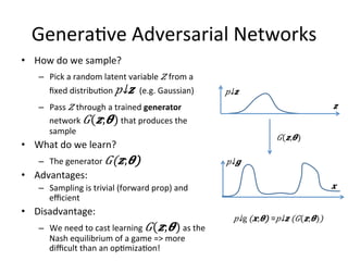
This document provides an introduction to generative adversarial networks (GANs). It discusses how GANs work by framing image generation as a game between a generator network that produces images and a discriminator network that evaluates them. The generator is trained to produce more realistic images that can fool the discriminator while the discriminator is trained to better distinguish real from generated images. GANs allow generating new images in one step by passing random noise to the trained generator network.

1. Introduc)on to
Genera)ve Adversarial Nets
Stefan Mathe

2. Roadmap
1. What are genera)ve models?
2. Mo)va)on
3. A Taxonomy of genera)ve models
4. Genera)ve Adversarial Nets (GANs)
1. Model Defini)on
2. Theore)cal Guarantees
3. Generaliza)ons
4. Evalua)on
5. Conclusions

3. What are Genera)ve Models?
• Input: a training set of samples drawn from a
distribu)on ​𝑝↓data
• Output: an es)mate of ​𝑝↓data
– How do we represent it?

4. Represen)ng ​𝑝↓𝑑𝑎𝑡𝑎
as a probability
density func)on
as a sample
generator
training
samples
model
generated
samples

5. Mo)va)on

6. Why study genera)ve models?
• Model Based Reinforcement Learning
• Semi-supervised Learning
• Handling mul)-modal outputs
• Generate realis)c samples
– Single image super-resolu)on
– Crea)ng art
– HandwriTen Digit Genera)on
– Image-to-image transla)on

7. Single Image Super-Resolu)on
Ledig et al. (2016)
original bicubic interpola)on SRResNet SRGAN
SRResNet: Super-resolu)on ResNet
SRGAN: Super-resolu)on SRGAN mul)-modal response => not blurry!

8. Crea)ng Art: Interac)ve GAN (iGAN)
Zhu et al. (2016)
hTps://www.youtube.com/watch?v=9c4z6YsBGQ0

9. Crea)ng Art: Interac)ve GAN (iGAN)
Zhu et al. (2016)
hTps://www.youtube.com/watch?v=9c4z6YsBGQ0

10. HandwriTen Digit Genera)on
Kingma and Welling (2013)
hTp://dpkingma.com/sgvb_mnist_demo/demo.html

11. Image-to-image Transla)on
Isola et al. (2016)

12. A Taxonomy of Genera)ve
Models

13. Maximum Likelihood (ML)
​𝜽↑∗ =​​arg max┬𝜽 ⁠∑𝑖=1↑𝑛▒log(​​𝑝↓model ↑𝜽
(​𝒙↓𝑖 ))
Figure reproduced from Goodfellow et al. (2016)

14. ML and the
Kullback Leibler (KL) divergence
• Our training samples define an empirical
distribu)on ​​𝑝 ↓data
​​𝑝 ↓data (𝑥)=∑𝑖=1↑𝑛▒​1↓​𝑥↓𝑖 (𝑥)
​𝜽↑∗ =​​arg min┬𝜽 ⁠​𝐷↓𝐾𝐿 (​​𝑝 ↓data ‖​
𝑝↓model )
• ML is equivalent to minimizing the KL
divergence between ​​𝑝 ↓data and ​𝑝↓model

15. A Taxonomy of Genera)ve Models
Genera)ve Model
Explicit Density Implicit Density
Tractable
Density
Approximate
Density
Direct Sampling
Markov Chain
Sampling
Fully Visible
Belief Nets
(FVBN)
Nonlinear
ICA
Varia)onal
Autoencoder
(VAE)
Boltzmann
Machine
Genera)ve
Adversarial
Nets (GAN)
Genera)ve
Stochas)c
Networks (GSN)
Adapted from Goodfellow et al. (2014)
state-of-the-art

16. Explicit Density Models
• Explicitly represent ​𝑝↓model (𝒙;𝜽)
• Advantages:
– Easy to op)mize, just plug ​𝑝↓model into the ML objec)ve
– Can evaluate the likelihood of any sample, if needed
• Disadvantages:
– ​𝑝↓model must be complex enough => tractability issues
• Solu)on 1: restrict ​𝑝↓model to a tractable, but rela)vely strong,
family (FVBN, nonlinear ICA)
• Solu)on 2: approximate ​𝑝↓model (VAEs, Boltzmann Machines)
– Hard to generate new samples

17. Implicit Density Models
• Interact indirectly with ​𝑝↓model (𝒙;𝜽) by sampling
• Advantages:
– Sampling is straighiorward
• Disadvantages:
– Likelihood is expensive to compute
• Sampling procedures
– Itera)ve (GSNs):
• Learn the denoising distribu)on (ojen unimodal) via ML
• Pick a training sample, apply noise and denoise repeatedly
• Ajer enough itera)ons, we get a sample from ​𝑝↓data (𝒙)
– Direct (GANs)
• Sample in a single step
• Objec)ve func)ons

18. Genera)ve Stochas)c Networks
• How do we sample?
– Pick a random training example
– Apply noise and denoise repeatedly
– Ajer enough itera)ons, we get a sample from ​𝑝↓data (𝒙)
• What do we learn?
– the denoising distribu)on 𝑝​𝒙⁠​𝒙 via ML
• Advantages:
– Learning is cast as an op)miza)on problem
– 𝑝​𝒙⁠​𝒙 is known to be easy to learn
• Disadvantage:
– Sampling is expensive

19. Genera)ve Adversarial Networks
​𝑝↓g (𝒙;𝜽) =​𝑝↓𝒛 (𝐺(𝒛;𝜽))
​𝑝↓𝒛
𝒛
​𝑝↓𝒈
𝒙
𝐺(𝒛,𝜽)
• How do we sample?
– Pick a random latent variable 𝑧 from a
fixed distribu)on ​𝑝↓𝒛 (e.g. Gaussian)
– Pass 𝑧 through a trained generator
network 𝐺(𝒛;𝜽) that produces the
sample
• What do we learn?
– The generator 𝐺(𝒛;𝜽)
• Advantages:
– Sampling is trivial (forward prop) and
efficient
• Disadvantage:
– We need to cast learning 𝐺(𝒛;𝜽) as the
Nash equilibrium of a game => more
difficult than an op)miza)on!

20. Genera)ve Adversarial Training
• Formulate the problem as a game between:
– The generator ​𝑝↓g (𝒙;​𝜽↓𝒈 )=​𝑝↓𝒛 (𝐺(𝒛;​𝜽↓𝒈 )) (as
before)
– The discriminator 𝐷(𝒙;​𝜽↓𝒅 ): tries to determine whether
𝒙 was sampled from ​𝑝↓data
Figure reproduced from Goodfellow et al. (2016)

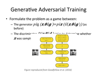
21. Genera)ve Adversarial Training
​​𝜽↓𝒈 ↑∗ =​​argmin┬​𝜽↓𝒈 ⁠​​max┬​𝜽↓𝒅 ⁠​𝔼↓𝑥~​𝑝↓data [​log⁠𝐷(𝒙;​𝜽↓𝒅 ) ] +​𝔼↓𝑧~​𝑝↓𝐳 [​
log⁠(1−𝐷(𝐺(𝒛;​𝜽↓𝒈 )) ]
• Formally:
Figure reproduced from Goodfellow et al. (2014)

22. Genera)ve Adversarial Training
• Cannot find the op)mum D for each G (too expensive)!
• Solu)on: Alternate between op)mizing G (keeping D fixed)
and op)mizing D (keeping G fixed) => a minimax game

23. Convergence Guarantees
• Only available for infinite capacity models
1. Minimax game has a global minimum at ​𝑝↓g =​
𝑝↓data
2. If 𝐷 is allowed to reach its op)mum in the inner
loop in the algorithm, then ​𝑝↓g →​𝑝↓data
• We don’t yet have sufficient theore)cal
support for the success of these models!

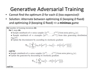
24. The Minimax Game (Generalized)
• D minimizes ​𝐽↑(𝐷) (​𝜽↓𝒈 ,​𝜽↓𝒅 ) w.r.t. ​𝜽↓𝒅 and
updates ​𝜽↓𝒅
• G minimizes ​𝐽↑(𝐺) (​𝜽↓𝒈 ,​𝜽↓𝒅 ) w.r.t. ​𝜽↓𝒈 and
updates ​𝜽↓𝒈
• For D, we always use the cross entropy:
​​𝐽↑(𝐷) =⁠−​𝔼↓𝑥~​𝑝↓data [​log⁠𝐷(𝒙;​𝜽↓𝒅 ) ]−​
𝔼↓𝑧~​𝑝↓𝐳 [​log⁠(1−𝐷(𝐺(𝒛;​𝜽↓𝒈 )) ]
• For G, in the minimax game:

25. Heuris)c non-satura)ng game
• Problem with minimax: when 𝐷 rejects generated
samples, G has no gradient!
• Solu)on: flip the target of the cross-entropy for G
​​𝐽↑(𝐺) =⁠​𝔼↓𝑧~​𝑝↓𝐳 [​log⁠(𝐷(𝐺(𝒛;​𝜽↓𝒈 )) ]
• G minimizes: ​𝐷↓𝐾𝐿 (​𝑝↓model ‖​𝑝↓data )−​2𝐷↓𝐽𝑆
(​𝑝↓data ‖​𝑝↓model )
• L Not nice (but it works!):
– No longer a 0-sum game
– Gets us even further from the theore)cal guarantees
• Recent work by Arjovski et. al. (2017) removes
the need for such tricks J (not presented here)

26. Maximum likelihood game
• It can be shown that the minimax game
op)mizes the Jensen-Shannon (JS) divergence
between ​𝑝↓data and ​𝑝↓model
• We can make the model op)mize the KL
divergence if we set
​​𝐽↑(𝐺) =⁠​−𝔼↓𝑧~​𝑝↓𝐳 [​log⁠(​𝜌↑−1 (𝐺(𝒛;​𝜽↓𝒈 )) ]

27. Quan)ta)ve Evalua)on
• How to compare models?
– Problem: log likelihood not easy to compute for genera)ve
machines
– Solu)on: es)mate via Parzen Windowing
• At least comparable to other methods on MNIST,
TFD

28. Qualita)ve Comparison
• Non-trivial, sharp solu)ons (not memorizing data)
MNIST TFD
CIFAR-10 (fully connected) CIFAR-10 (conv D, deconv. G)

29. What makes GANs work?
(Give sharper results than VAEs)
• Ini)al hypothesis:
– because they minimize JS instead of KL
– KL is not symmetric, minimizing JS similar to reverse KL
• Not true!
– ML GANs s)ll generate sharp results
– GANs prefer far fewer modes than G’s capacity would allow
• Mistery solved recently by Arjovski et. al. (2017)”:
– Both JS and KL induce convergence issues
– There is a probability measure to use
Figure reproduced from Goodfellow et al. (2016)

30. The Convergence Problem
• We only have theore)cal guarantees for convergence in
func)on space
• Typical failure: mode collapse (the Helve4ca Scenario)
• Hypothesis: maximin different from minimax, but the
associated games (simultaneous descent) are almost
iden)cal!
​​min┬​𝜽↓𝒈 ⁠​​max┬​𝜽↓𝒅 ⁠𝑉(​𝜽↓𝒈 ,​𝜽↓𝒅 ) ≠ ​​max┬​𝜽↓𝒅 ⁠​​min┬​𝜽↓𝒈 ⁠𝑉(​𝜽↓𝒈 ,​𝜽↓
Figure reproduced from Goodfellow et al. (2016)

31. Conclusions
• Contribu)on: GANs completely break away from the ML
approach by switching to an adversarial mini-max game
formula)on
• Strengths:
– Easy and efficient sample genera)on process
– Simple training algorithm
– No need for a noise model
– State-of-the art results (qualita)vely the best)
• Weaknesses:
– No explicit likelihood representa)on
– Convergence problems (Helve)ca scenario)
– Model comparison issues (Parzen Windows, high variance)
– We don’t know why they work (no theore)cal guarantees)
• But see: Arjovski et. al. (2017)” for a recent and elegant
solu)on for the former two!

32. Stop GAN Violence!
While the costs of human violence have aFracted a great deal of aFenGon from
the research community, the effects of the network-on-network (NoN) violence
popularised by GeneraGve Adversarial Networks have yet to be addressed. In this
work, we quanGfy the financial, social, spiritual, cultural, grammaGcal and
dermatological impact of this aggression and address the issue by proposing a
more peaceful approach which we term GeneraGve Unadversarial Networks
(GUNs). Under this framework, we simultaneously train two models: a generator
G that does its best to capture whichever data distribuGon it feels it can manage,
and a moGvator M that helps G to achieve its dream. FighGng is strictly verboten
and both models evolve by learning to respect their differences. The framework is
both theoreGcally and electrically grounded in game theory, and can be viewed
as a winner-shares-all two-player game in which both players work as a team to
achieve the best score. Experiments show that by working in harmony, the
proposed model is able to claim both the moral and log-likelihood high ground.
Our work builds on a rich history of carefully argued posiGon-papers, published as
anonymous YouTube comments, which prove that the opGmal soluGon to NoN
violence is more GUNs.
Albanie et al. arXiv:1703.02528, 2017

33. Resources
• Code and pretrained model:
– hTps://github.com/goodfeli/adversarial
• Tutorial:
– hTps://arxiv.org/pdf/1701.00160.pdf

34. References
• [1] I. Goodfellow, J. Pouget-Abadie, M. Mirza, B. Xu, D. Warde-Farley, S.
Ozair, A. Courville and Y. Bengio. “Genera)ve Adversarial Nets”, NIPS,
2014.
• [2] I. Goodfellow, ”Genera)ve Adversarial Networks”, NIPS 2016 Tutorial
• [3] M. Arjovsky, S. Chintala, L. BoTou, “Wasserstein GAN”, ArXiV
1701.07875v2, 2017
• [4] S. Albanie, S. Ehrhardt, J. F. Henriques, “Stopping GAN Violence:
Genera)ve Unadversarial Networks”, ArXiV 1703.02528v1, 2017