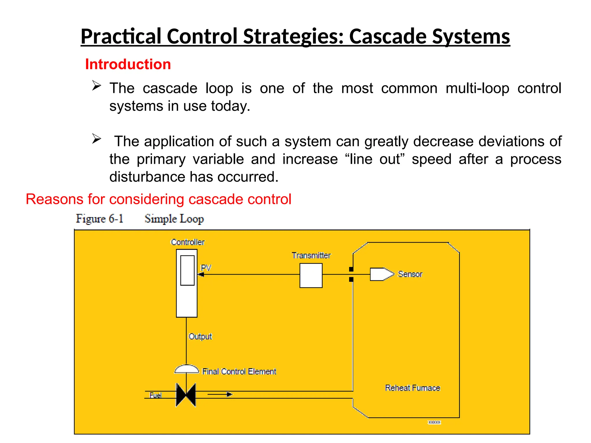
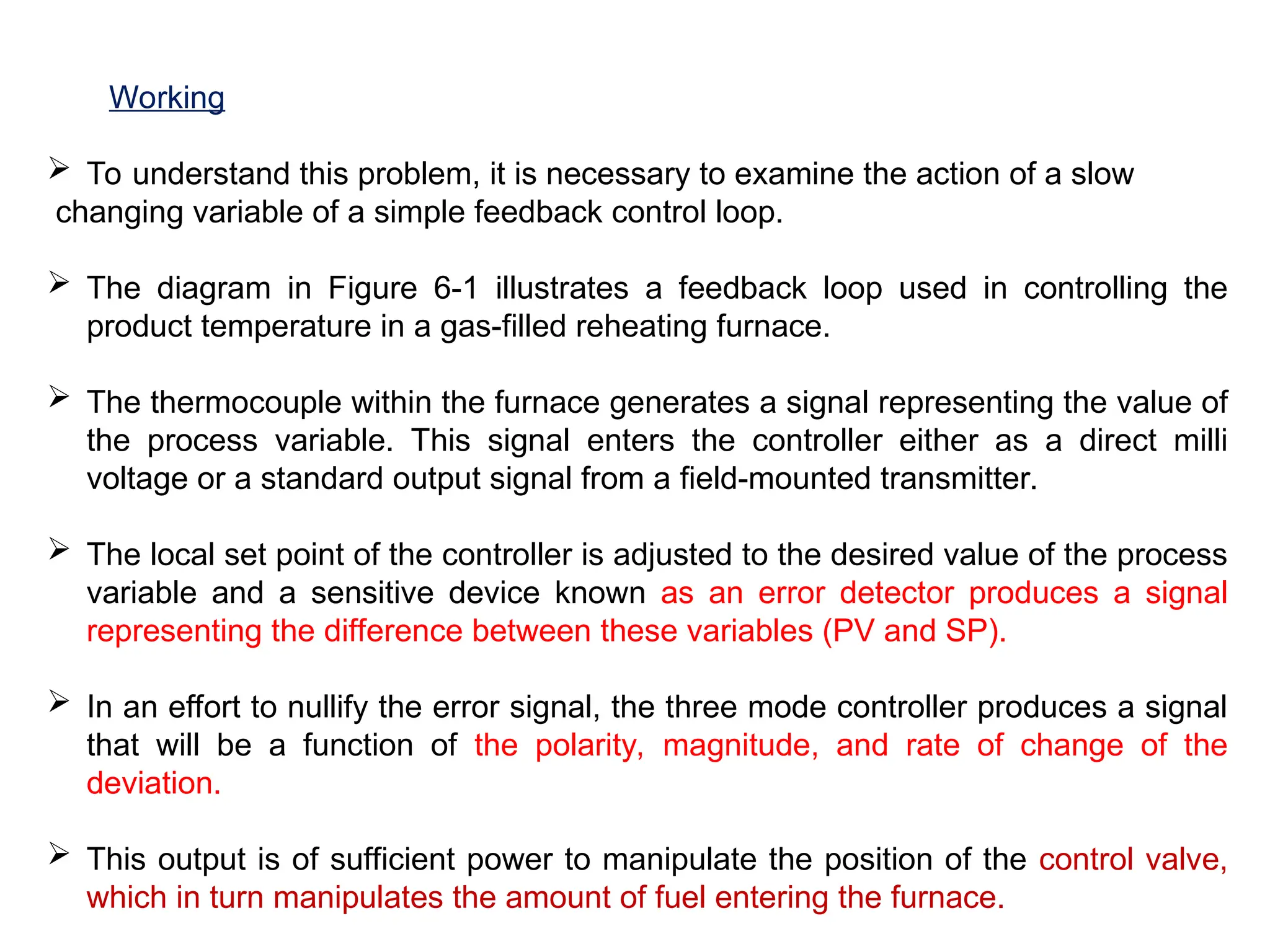
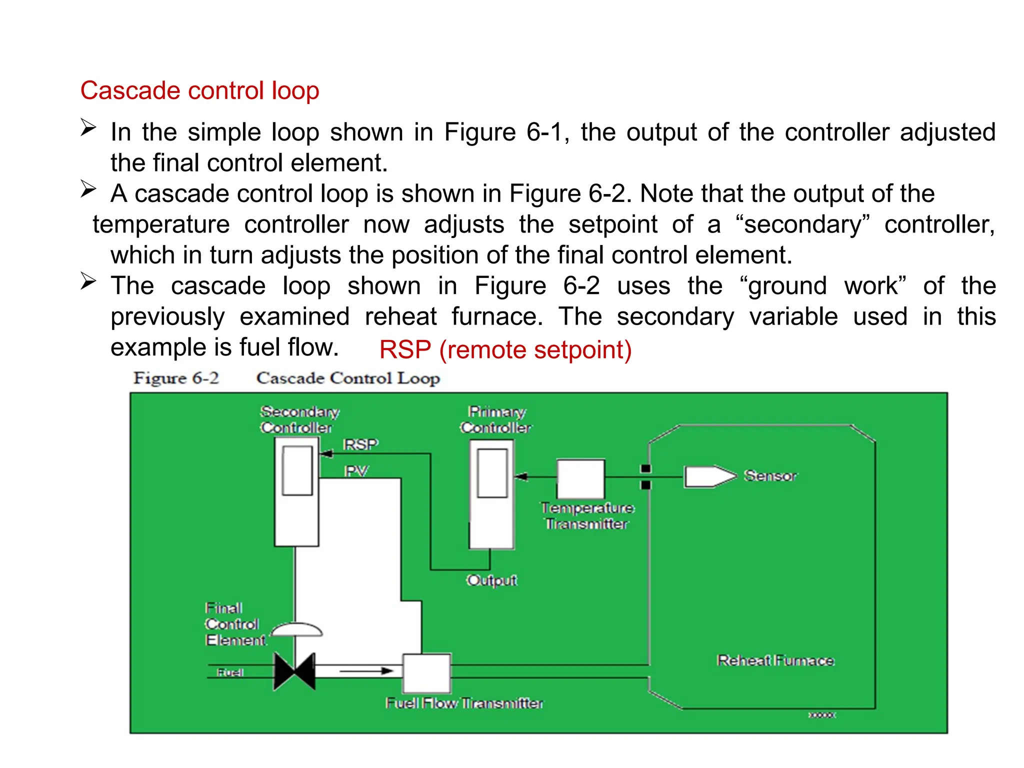
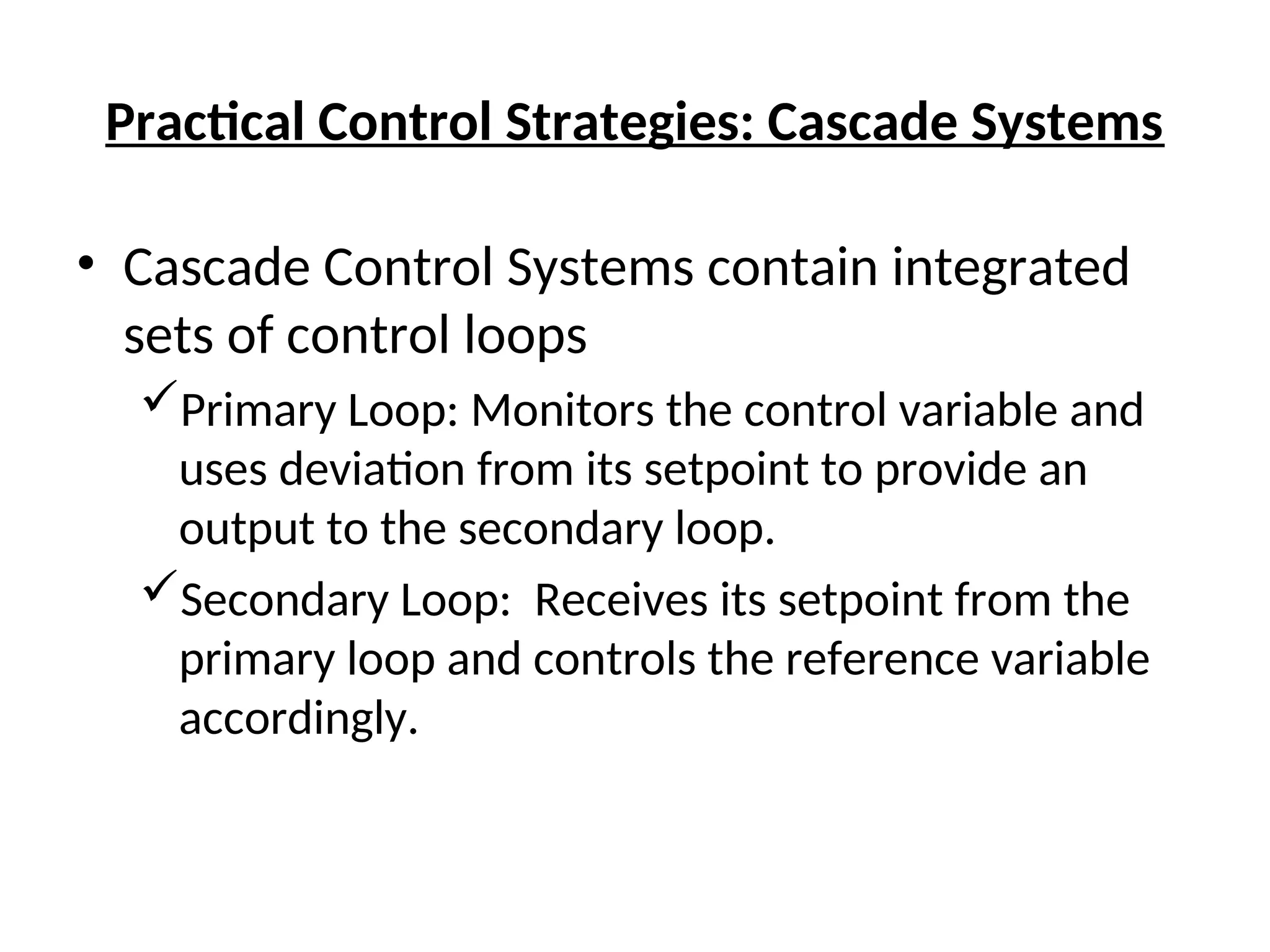
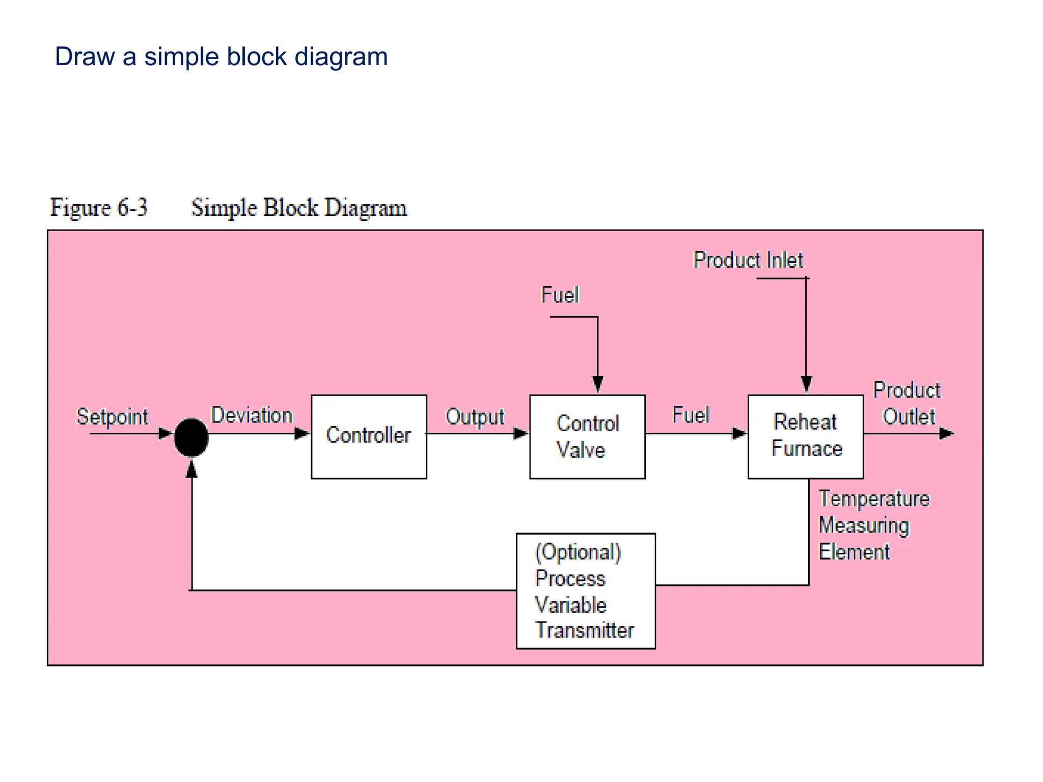
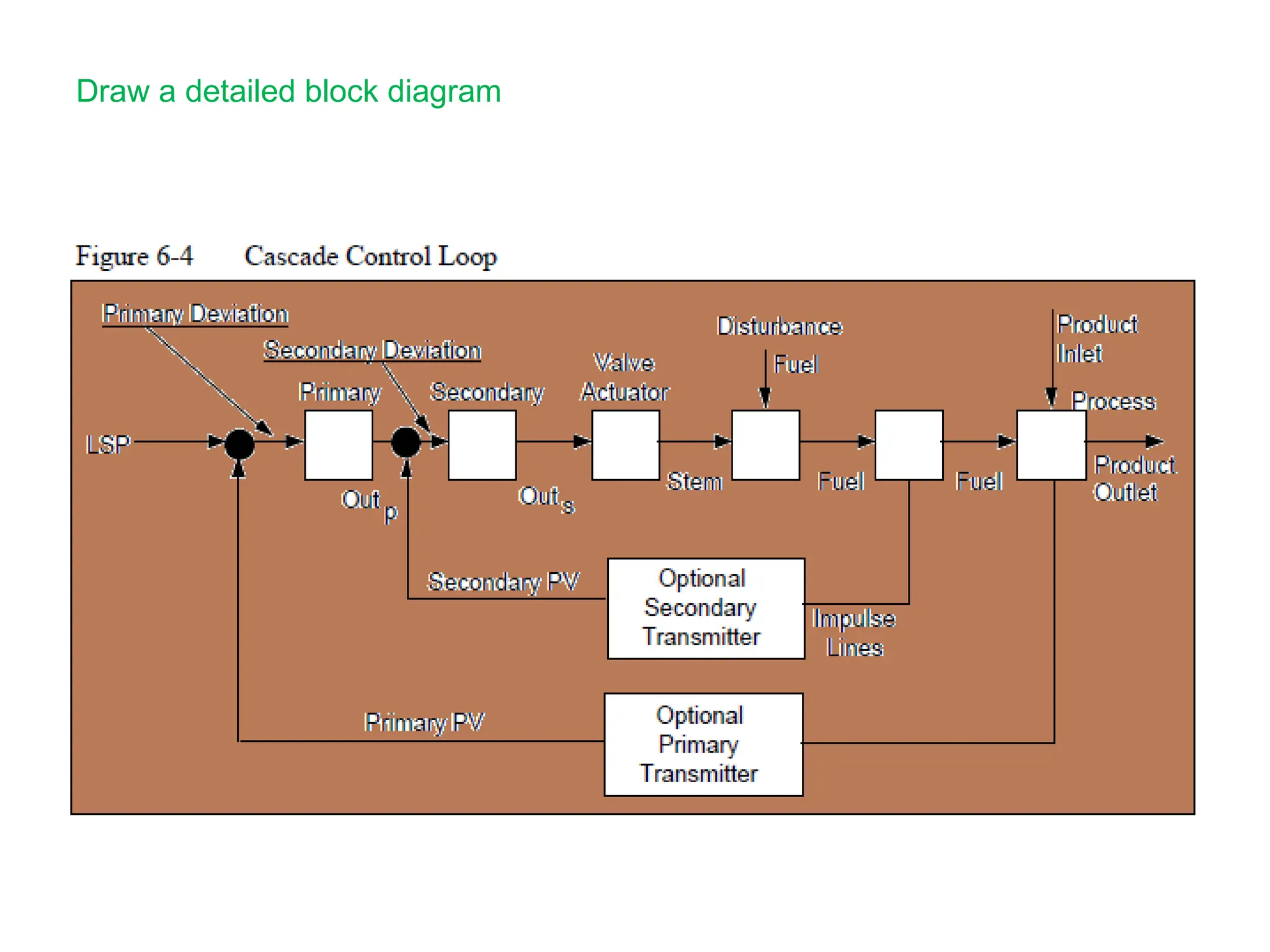
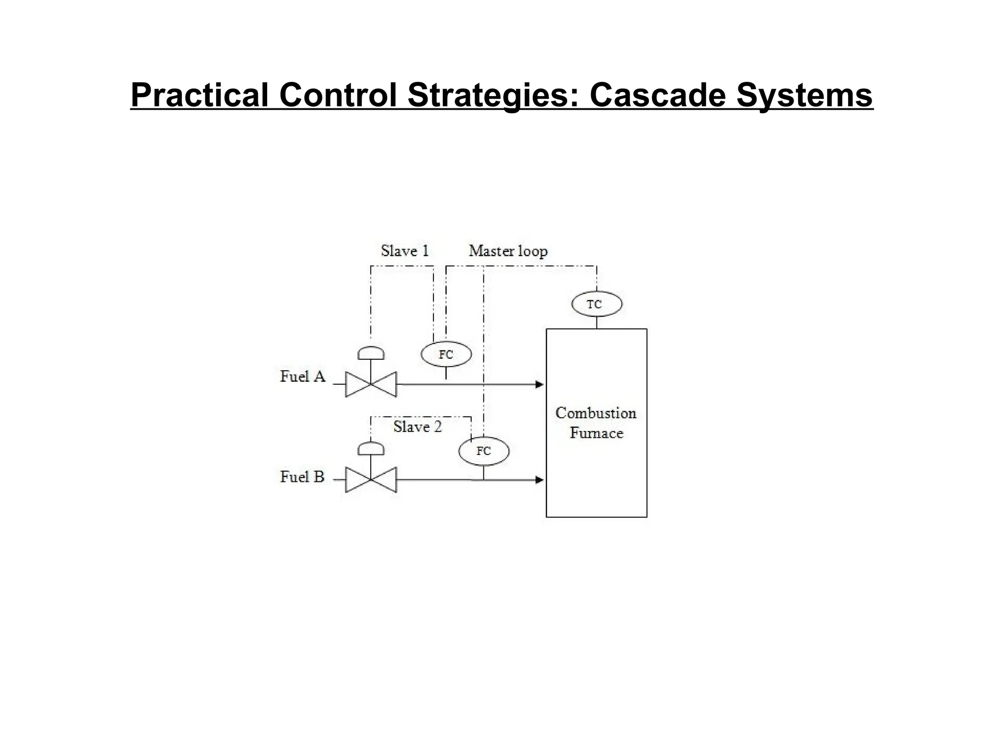
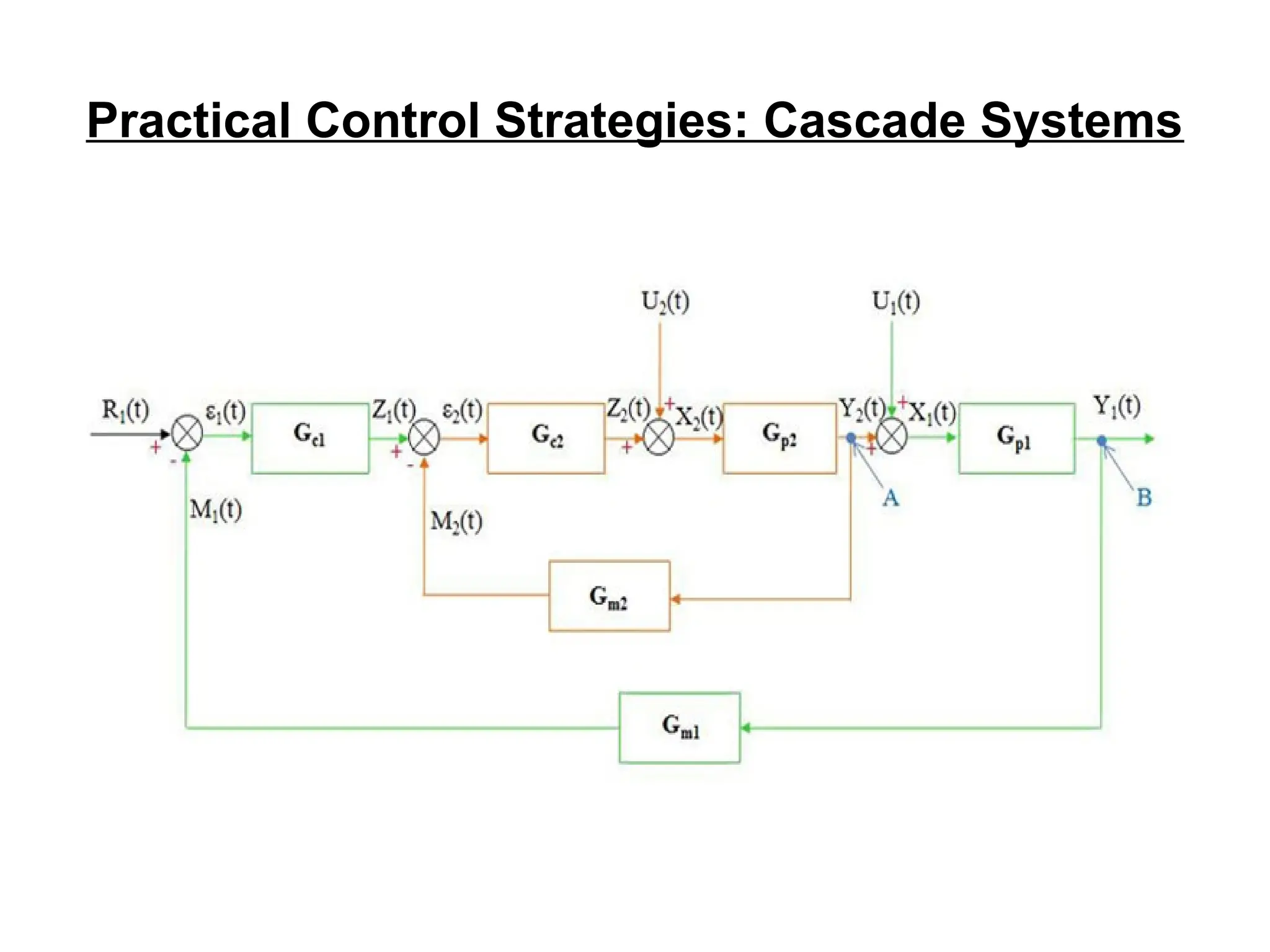
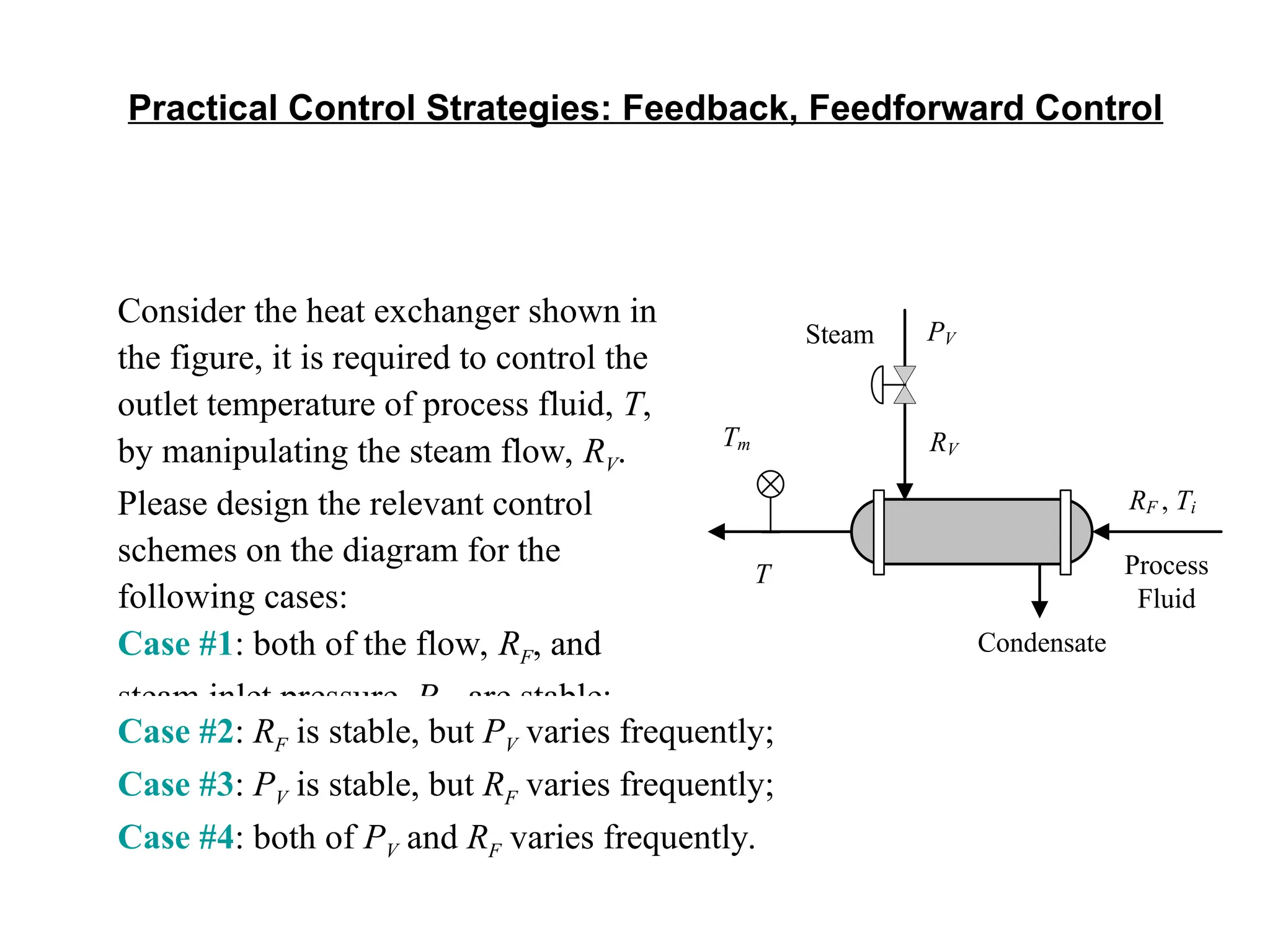
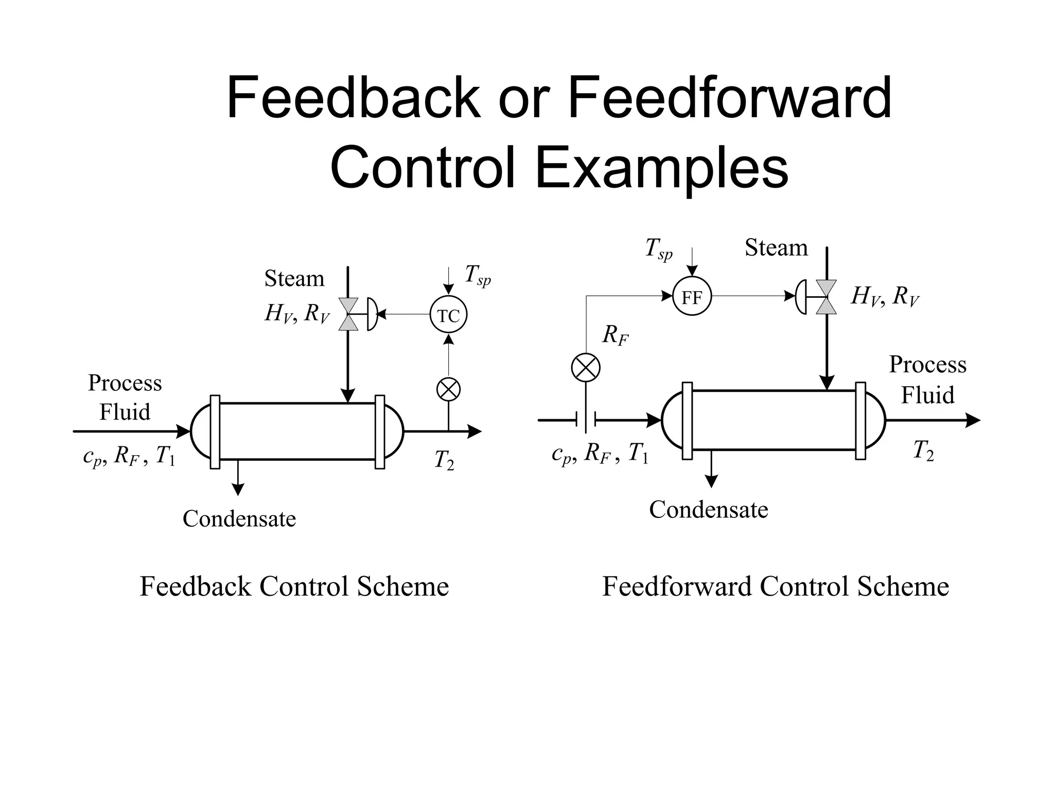
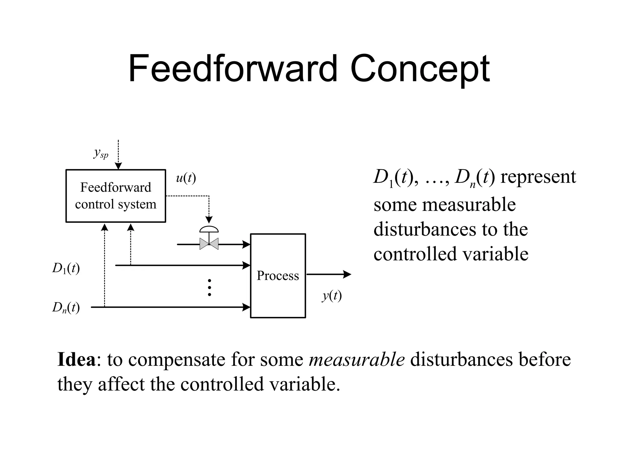
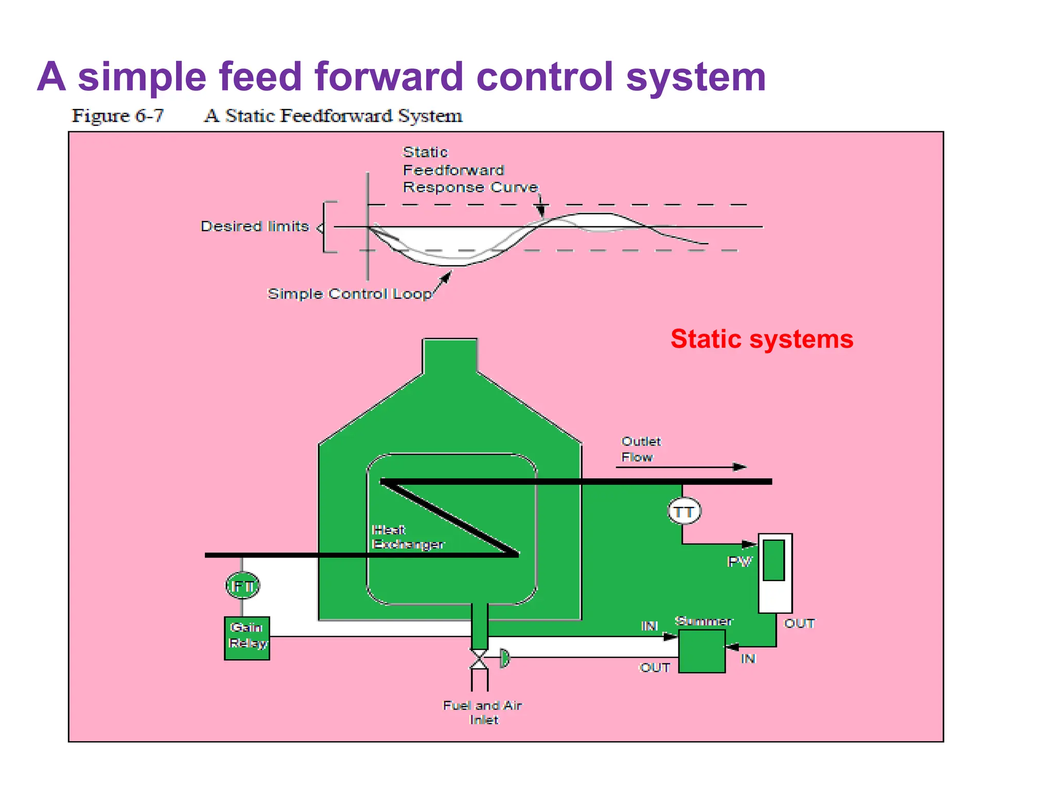
Fundamental process control system Chapter2.ppt

Process Control
Fundamentals
Dr. Amruth RT

Course Overview (2/5)
Chapter 2: Practical Control Strategies
1. Cascade Control
2. Ratio Control
3. Dead Time Control
4. Feedforward Control
5. Feedback Control

Practical Control Strategies: Cascade Systems
Introduction
 The cascade loop is one of the most common multi-loop control
systems in use today.
 The application of such a system can greatly decrease deviations of
the primary variable and increase “line out” speed after a process
disturbance has occurred.
Reasons for considering cascade control

Working
 To understand this problem, it is necessary to examine the action of a slow
changing variable of a simple feedback control loop.
 The diagram in Figure 6-1 illustrates a feedback loop used in controlling the
product temperature in a gas-filled reheating furnace.
 The thermocouple within the furnace generates a signal representing the value of
the process variable. This signal enters the controller either as a direct milli
voltage or a standard output signal from a field-mounted transmitter.
 The local set point of the controller is adjusted to the desired value of the process
variable and a sensitive device known as an error detector produces a signal
representing the difference between these variables (PV and SP).
 In an effort to nullify the error signal, the three mode controller produces a signal
that will be a function of the polarity, magnitude, and rate of change of the
deviation.
 This output is of sufficient power to manipulate the position of the control valve,
which in turn manipulates the amount of fuel entering the furnace.

Drawback
In this simple control loop, the system has been designed to control the process
variable (temperature) by valve adjustment, although heat supply is actually the
factor determining the temperature
 A system which helps to overcome the serious time delays and poor control
caused by fuel pressure and flow disturbances is called cascade control.
Reasons to choose Cascade Controller
In this example, fluctuations in fuel pressure created variations in the fuel flow.
As the flow of fuel to the furnace changed, so did the amount of energy.
 The pressure fluctuations resulted in temporary deviations of the process
variable, which could not be controlled adequately using only the simple
feedback control loop.
Avoiding the deviations was not possible because the disturbance entered the
system without being detected, and once the error began developing, corrective
action was initiated too late.

Cascade control loop
 In the simple loop shown in Figure 6-1, the output of the controller adjusted
the final control element.
 A cascade control loop is shown in Figure 6-2. Note that the output of the
temperature controller now adjusts the setpoint of a “secondary” controller,
which in turn adjusts the position of the final control element.
 The cascade loop shown in Figure 6-2 uses the “ground work” of the
previously examined reheat furnace. The secondary variable used in this
example is fuel flow. RSP (remote setpoint)

• Cascade Control Systems contain integrated
sets of control loops
Primary Loop: Monitors the control variable and
uses deviation from its setpoint to provide an
output to the secondary loop.
Secondary Loop: Receives its setpoint from the
primary loop and controls the reference variable
accordingly.

How it works
 If the temperature of the product within the furnace is too high, the primary
controller lowers its output, requesting a decrease in the fuel flow setpoint.
 If the temperature drops, the device raises the setpoint of the secondary controller,
which in turn increases the fuel flow to match its new setpoint.
 In any case, the primary controller is controlling temperature by adjustments in the
secondary controller’s setpoint.
 Since the secondary controller is designed to measure and control fuel flow, the
primary controller adjusts fuel flow, not valve position.
 Therefore, when a flow disturbance occurs, the fuel flow transmitter will notice it
before it can adversely affect the process.
 The secondary controller will quickly readjust the valve position until flow once
again matches the setpoint dictated by the primary.

Secondary control loop
 The secondary control loop consists of a simple flow loop. This controller
measures the flow of fuel and compares it to the value desired by the primary
controller.
 The function of the controller is to maintain the flow at the remote setpoint it
receives.
 Note that with this configuration, deviations due to fuel should increase, there
will be a rise in fuel flow rate.
 Before this increased flow affects the temperature, it is detected by the
secondary transmitter and thus, the secondary controller.
 In an attempt to maintain a zero error between its PV and RSP (remote setpoint),
the secondary controller quickly changes its output in a direction to reduce the
fuel flow and reestablish a zero error.
 Because of the speed of response of this variable, as compared to that of the
primary, the temperature changes very little.

How to choose a secondary variable
 In the cascade control loop previously introduced, it was noticed that the
selection of fuel flow as a secondary variable was a good one.
 It should be obvious that to obtain the maximum benefits from a cascade
control system, a wise choice of the secondary variable is a vital requirement.
 How does one choose the most appropriate secondary variables?
 Application engineers have developed some “rules of thumb” for choosing
the optimum secondary variable.

• Effectively accounts for external disturbances
• Reduces dead time in variable response
• Compatible with other Control Systems, such
as Feed-Back and Feed-Forward Control
Architectures
Practical Control Strategies: Benefits of
Cascade Systems

Rules for determining secondary elements and variables
After the diagram has been made, plan possible alternates for placement of the
secondary measuring element and selection of the secondary variable, using these
five rules.
1. Make the secondary loop include the input point of the most serious disturbances.
It is the effect of these disturbances which the cascade loop must be most successful
in controlling.
2. Make the secondary loop fast by including only minor lags. When comparing the
speed of response of the primary variable (TP) to that of a possible secondary
variable (TS), the ratio of TP/TS should preferably be at least 3. Ratios of 5 or 10 are
even more desirable.
3. Use a secondary variable with setpoint values that are definitely related to the
value of the primary variable. In undisturbed operation of the system, at line out, the
relationship of the secondary setpoint to the primary variable should be represented
by a single line. If the line is relatively straight rather than curved, this will simplify the
tuning of the primary controller.
4. If the secondary loop can remain relatively fast (see note 2), make it contain as
many of the disturbance inputs as possible. The improvements in close control after a
disturbance has entered a cascade control loop will be roughly related to the gain
settings of both controllers.

• Multiple control loops make physical and
computational architecture more complex
• Additional controllers and sensors can be
costly
Practical Control Strategies: Disadvantages of
Cascade Systems

Consider the heat exchanger shown in
the figure, it is required to control the
outlet temperature of process fluid, T,
by manipulating the steam flow, RV.
Please design the relevant control
schemes on the diagram for the
following cases:
Case #1: both of the flow, RF, and
steam inlet pressure, PV, are stable;
T
RV
RF , Ti
Steam
Condensate
Process
Fluid
PV
Tm
Case #2: RF is stable, but PV varies frequently;
Case #3: PV is stable, but RF varies frequently;
Case #4: both of PV and RF varies frequently.
Practical Control Strategies: Feedback, Feedforward Control

Feedback or Feedforward
Control Examples
TC
cp, RF , T1 T2
HV, RV
Steam
Process
Fluid
Condensate
Tsp
cp, RF , T1 T2
HV, RV
FF
RF
Steam
Process
Fluid
Condensate
Tsp
Feedback Control Scheme Feedforward Control Scheme

Feedforward Concept
Process
y(t)
u(t)
...
Dn(t)
D1(t)
ysp
Feedforward
control system
D1(t), …, Dn(t) represent
some measurable
disturbances to the
controlled variable
Idea: to compensate for some measurable disturbances before
they affect the controlled variable.

Feedforward / Feedback Control
Process
y(t)
u(t)
D(t)
ysp Feedforward
control system
Feedforward
control system
ysp
∑
+ +

Feedforward Plus Feedback Control
System

Design of Linear Feedforward
Controllers
Process
y(t)
u(t)
D(t)
ysp
Feedforward
control system
＋
＋
D (t)
ym (t)
Disturbance
Measurement
GDM (s)
Feedforward
Controller
GFF (s)
Dm (t) u(t) Control Path
GYC (s)
Disturbance Path
GYD (s)
Extended Controlled Process
Design Objective:
( )
( ) ( ) ( ) ( )
( )
0
m
YD YC FF DM
Y s
G s G s G s G s
D s
 


Controllers (cont.)
Design formula for the feedforward
controller:
( )
( )
( ) ( )
YD
FF
YC DM
G s
G s
G s G s

＋
＋
D (t)
ym (t)
Disturbance
Measurement
GDM (s)
Feedforward
Controller
GFF (s)
Dm (t) u(t) Control Path
GYC (s)
Disturbance Path
GYD (s)
Extended Controlled Process
Design Objective:
( )
( ) ( ) ( ) ( )
( )
0
m
YD YC FF DM
Y s
G s G s G s G s
D s
 


Controllers (cont.)
Design formula for the feedforward controller:
( )
( )
( ) ( )
YD
FF
YC DM
G s
G s
G s G s

 
s
s
T
K
s
G D
YD
YD
YD 


 exp
1
)
(  
s
s
T
K
s
G C
YC
YC
YC 


 exp
1
)
(
DM
DM K
s
G 
)
(
 
s
s
T
s
T
K
s
G FF
YD
YC
FF
FF 



 exp
1
1
)
(
DM
YC
YD
FF
K
K
K
K 
  
C
D
FF 

 
 ,
0
max ( Why ? )

Comparison of Feedforward
and Feedback Control
Feedforward Control Feedback Control
Disturbances are measurable CV is measurable
Control MV based on
disturbances
Control MV based on control
ERROR
Open-loop, No Stability
Problem
Closed-loop, Stability is the
most important
Only some disturbances are
detected
All disturbances are detected
Accurate model needed for
both of Control and
Disturbance Paths
No accurate model needed
Not adaptable to nonlinear or
time-varied systems
Adaptable to nonlinear or
time-varied systems

Predictive Feed forward Control
Introduction
 In the previous section, cascade control systems were discussed.
 In these systems, the disturbance was noticed by the secondary sensor and
controller, and brought under control before it could adversely affect the primary
variable.
 For cascade control to be a suitable option, the variable which is creating the
disturbance (the secondary variable) must be controllable.
 For example, in the reheat furnace of the previous discussion, the changes in
fuel flow were causing process upsets. In this example, fuel flow could be
controlled.
 In other words, it can be sensed by the secondary transmitter, and controlled in
an on-going fashion by the secondary controller which manipulates the final
control element.
 It is the disturbed variable’s ability to be measured, compared to a remote
setpoint, and continuously corrected by a final control element which makes it
suited for cascade control.

When to use feed forward control
 In some applications, a disturbance takes place which cannot be controlled
(although it can be measured).
 An example of such an application could be the disturbance in the feed rate of
product through a heat-exchanger.
 In this case, cascade control could not be used. However, a system called
feed forward can anticipate and compensate for the disturbance, although control
of the disturbance is not possible.
 The simple loop and the cascade loop are both types of “feedback” control.

 There are several inherent limitations to feedback control, which the feed
forward system improves upon:
• All feedback control systems obtain control by measuring the error and
supplying a restoring output. The system depends on an error to generate a
corrective signal. Without the error, the controller output is stable. When the
error becomes evident, the controller must slowly integrate for correction.
With a steady state error, gain and derivative cease to offer a contributing
factor to the output.
• All feedback control systems obtain the correct output by trial and error. The
system will never know the correct output necessary to solve the problem.
The basic operation of the system is shown in Figure 6-5.

 The simple flow diagram shown in this figure assumes that the controller output is
changing in the correct direction.
 Some degree of oscillation is common in any trial and error attempt at control.

An approach to feedback problems
 To find methods of solving some of the problems existing with feedback
control systems, one would begin by considering a different approach.
 The approach would be to measure the principle factors that affect the
process, and calculate the correct output to meet current conditions.
 If a disturbance should occur, information will be fed to the final control
device before the system senses that a problem has arrived.
 A flow diagram depicting this concept might appear as shown in Figure 6-6.

Note that in Figure 6-6, the system has no “return” of information.
 The correct output value is computed by changes in the setpoint, process
variable, or fluctuations of external system disturbances.
The process of feeding this information forward to compute the correct
output value is known as FEEDFORWARD.
Essential Feature of Predictive Feed forward Control
The essential feature which distinguishes this system from feedback control
loops is the forward flow of information.
The feedforward scheme can produce tremendous improvements in control
because in practice, it continuously balances the material or energy requirements
of the process against the current demands of the load.

A simple feed forward control system
Static systems

Figure 6-7 depicts a simple feedforward control system.
 The loop is of the continuous form, wherein liquid is fed through a heat exchanger
and is heated to a desired value.
The controller output feeds the final control element through a summation
auxiliary.
 The auxiliary is an analog adder that sums the values of its inputs.
The feed forward transmitter measures inlet flow to the heat exchanger, and its
output is multiplied by the setting on the adjustable gain relay.
The resulting feed forward signal becomes the second input to the summer.
If the influent feed rate should increase, the flow transmitter instantly feeds an
increase signal to the summer.
The magnitude of this signal will depend on the degree of feed flow increase and
the gain set on the relay.
The feed forward signal will increase the output from the summer andproduce an
immediate change in valve position.
The increased fuel inlet can now prevent large deviations of the feed temperature
from occurring.

Static systems
Feedforward strategies that compute corrective output values in a manner
independent of time are known as static systems.
The computed output was instantaneous and is designed to anticipate
current demand changes.
Figure 6-7 is an example of a static system.

Dynamic Feed forward Control
Introduction
Applications often exist, as in the previous example, where
predictive
Feed forward strategies will offer a dramatic improvement in control of
the
process variable.
Yet, even more improvement is sometimes obtainable by using Dynamic
Feed forward.
Illustration of dynamic
feedforward control|

How it works
 Assume that the increase of inlet feed had a much greater effect on
product temperature.
 The alternative, in the static system, would be to increase the gain of the
adjustable gain relay to cause a greater change in valve position.
The stronger initial correction signal could create overcorrection—opening the
valve too much, and causing a larger upset in the opposite direction.
 This deviation would have to be removed by the temperature controller.
The dynamic feedforward control system can provide more correction than the
static system, yet not create the undesired overcorrection.
With dynamic (or time variable) feedforward, the corrective signal will be
momentarily large, then gradually cut back.
 By gradually cutting back the corrective signal, the process will not experience a
large, sustained release of energy and overcorrection can be eliminated.
The “time dependent” feedforward signal can be generated by another auxiliary
device known as a Lead/Lag relay.

The Ratio Control Loop
In many control applications, there are two or more inputs to a process
which must be varied and controlled to meet process demand.
 The value of these variables (most often two flows) must be kept in a
prescribed ratio to achieve a particular end product. The system which
maintains this ratio is known as a ratio control loop.
 Some examples of ratio applications could be blending a base product
with a thinner, water, and foaming agent, or air and fuel.
Ratio control might be used where a continuous process is going on
and an additive is being put into the flow (e.g., chlorination of water).

Ratio control configurations
There are two ratio control configurations that are commonly used:
oSeries and
oParallel configurations.
There are definite advantages in choosing one over the other.

Series configuration
The Series system takes a “lead and follow” approach. According to the
demand of the process, a master controller will control one of the variable
(the “leader”) to a particular value.
The “follower” variable will then be controlled by a remote setpoint controller
to some predetermined ratio of the leader.
This means that as the first input variable rises, so will the value of the
second. If the leading variable falls to zero, so must the follower.
This interaction is the primary characteristic of the series ratio system.
 These systems can be characterized by a definite interlock between the
two controlled variables. This interlock can become a valuable safety feature.

•The master controller, measuring the consistency of the final product
blend, establishes the value of flow B.
•The flow is measured and its percentage equivalent becomes the setpoint
of the flow A controller.
•Controller A is by necessity a remote setpoint controller, identical to the
“secondary” controller of any cascade system.
• If flow B is 20%, then 20% becomes the setpoint for flow A.
Notice that in Figure 6-9, the pipe for flow A is much larger than B.
 This will allow a “pre-set” ratio to be established.
For example, if the range of operation of pipe A is 0 to 1000 cfh and pipe B is 0
to 500 cfh, the A:B ratio of maximum flow capacity would be 2:1.
The 20% fluid flow in pipe B would be 100 cfh, but in pipe A the flow
would be 200 cfh.

Since the value of A will be established by the value of B, the system is
serial.
The ratio of flow is fixed by the scale ranges of both variables and cannot
be changed without a major change in system hardware.
 If pipe A and B were the same size, the system shown in Figure 6-9 would
only be capable of maintaining a 1:1 ratio, since there is no device in the
system to multiply or divide flow B by some gain factor before sending it as a
remote setpoint to controller A.
Series system with ratio relays

•This system provides one major advantage over the previous example.
• By using a device known as a ratio relay between the flow in pipe B
and the flow A controller, the system will operate the same as example
A, except that the ratio of the flows can be easily adjusted.
For example, if pipe A and pipe B are the same size, and the ratio
relay is set at “2”, then flow A will be twice as great as flow B.
If pipe A is twice the size of pipe B, and the ratio relay is set at “2”,
then flow A will be four times as great as flow B.
If pipe A is one-third (.33) as great as pipe B, and the ratio relay is set
at “.5”, then flow A will be (.33 x .5) or .165 times flow B, or about one-
sixth of B.

Parallel systems Configuration
The parallel approach to ratio control allows the master controller to
set the value of both variables.
 Instead of one control system leading and the second one following, the
parallel concept ties both systems to the direct command of the master.
As process demand changes, the master controller adjusts the values of
both control systems simultaneously.
Since both systems receive their set points from the master controller, they
will respond to a change at the same time.
 How well the two systems are kept together will depend upon the
response characteristics of each.

Advantages of parallel ratio control
One of the advantages of parallel ratio control is that any noise occurring in the
“leader” variable will not be reflected in the “follower”.
Without the interlock, both systems are independent of one another.
This configuration can lead to yet another advantage. The simultaneous updating of
both systems could result in a smaller deviation from the desired ratio during changes
in process demand.
 The obvious disadvantage is loss of interlock safety. If one variable of a parallel
system drops to zero, the second will not.

Block diagrams of parallel ratio systems

Parallel ratio system function
This ratio control system has been designed so that instead of the master
controller setting the value of flow B only, the master controller sets the
flow values of both controllers.
Note that while in the series ratio system, the input to the ratio relay came
from the flow B transmitter/square root extractor, in this system, the input
to the ratio relay comes directly from the master controller.
 In the series ratio system, the RSP to controller A did not change until
flow B actually changed, not when the master controller merely called for a
change in flow B.
In the parallel ratio system, the RSP to Controller A changes the moment
the master controller calls for it.

Ratio relay adjustment
 The ratio of the two flows will be determined by the ratio relay
adjustment.
 Since the master controller sends both setpoint commands in a parallel
fashion to the flow controllers, both controllers will respond to a change at the
same time.
 How well the flows track each other over changes in demand will again be
determined by the two response characteristics.
Parallel system disadvantage
The parallel system will, in most cases, result in a better ratio control as
process load changes occur.
The basic disadvantage is the lack of flow interlock. If flow A should fall to zero
in a fault condition, flow B will not be affected.
Note that if an application arises where process personnel would like to
momentarily interrupt one of the flows without affecting the other, this non-
interlocked parallel system would offer such a possibility.

Ratio system with interlock
Some applications require that the ratio between the two flows never
exceeds a set value in one direction, because the result may represent an
uneconomical or unsafe condition.
A typical example of this is the air/fuel mixture in a burner. To keep the
mixture from ever being too rich in fuel, an interlock system is used.
Example of ratio system with interlock
This system, shown in Figure 6-13, is capable of providing this form of interlock
through the use of signal selectors.
In this example, if we use “X” to represent the desired ratio and A and B to
represent the actual flows, then the ratio of the actual flow must be equal to or
greater than the desired ratio.
This is how the system must perform:

If we assume that the desired ratio has been met (A = X) then to satisfy the
limits of the equation:
If a change in demand requires more of both fluids, note that to satisfy the
first rule, flow B cannot increase unless flow A increases first.
Conversely, to satisfy the second rule, if a decrease in both fluids is
necessary, flow A cannot decrease unless flow B does so first.

Fundamental process control system Chapter2.ppt

More Related Content

Similar to Fundamental process control system Chapter2.ppt

More from amruthramesh1

Recently uploaded

Fundamental process control system Chapter2.ppt