NYQUIST DIAGRAM

1. NYQUIST DIAGRAMS
• The Nyquist diagram is an alternative representation of frequency response
information, a polar plot of G(jω) in which frequency ω appears as an implicit
parameter.
• The Nyquist diagram for a transfer function G(s) can be constructed directly
from │G(jω) │ and G(jω) for different values of ω. Alternatively, the Nyquist
diagram can be constructed from the Bode diagram, because AR = │G(jω)│
and Ø= G(jω ).
• Advantages of Bode plots are that frequency is plotted explicitly as the
abscissa, and the log-log and semi-log coordinate systems facilitate block
multiplication.
• The Nyquist diagram, on the other hand, is more compact and is sufficient for
many important analyses, for example, determining system stability.

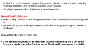
2. • Most of the recent interest in Nyquist diagrams has been in connection with designing
multiloop controllers and for robustness (sensitivity) studies.
• For single-loop controllers, Bode plots are used more often.
Nyquist Stability Criterion
• Bode Stability Criterion is valid for systems with AR and Ø monotonically decreasing with
ω
• For feedback systems with open loop Bode plots the more general Nyquist Criterion is
employed.
Nyquist Stability Criterion states that:
• If the open loop Nyquist plot of a feedback system encircles the point (-1,0) as the
frequency ω takes any value from -∞ to + ∞. The closed loop response is unstable.

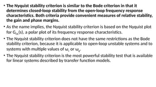
3. • The Nyquist stability criterion is similar to the Bode criterion in that it
determines closed-loop stability from the open-loop frequency response
characteristics. Both criteria provide convenient measures of relative stability,
the gain and phase margins.
• As the name implies, the Nyquist stability criterion is based on the Nyquist plot
for GOL(s), a polar plot of its frequency response characteristics.
• The Nyquist stability criterion does not have the same restrictions as the Bode
stability criterion, because it is applicable to open-loop unstable systems and to
systems with multiple values of ωc or ωg.
• The Nyquist stability criterion is the most powerful stability test that is available
for linear systems described by transfer function models.

4. Nyquist Stability Criterion.
• Consider an open-loop transfer function GOL(s)that is proper and has no
unstable pole-zero cancellations.
• Let N be the number of times that the Nyquist plot for GOL(s)encircles the
(-1, 0) point in the clockwise direction.
• Also let P denote the number of poles of GOL(s) that lie to the right of the
imaginary axis.
• Then, Z = N + P where Z is the number of roots (or zeros) of the characteristic
equation that lie to the right of the imaginary axis.
• The closed-loop system is stable if and only if Z = 0.

5. Important properties of the Nyquist stability criterion are:
• It provides a necessary and sufficient condition for closed-loop stability based
on the open-loop transfer function.
• The reason that the ( -1, 0) point is so important can be deduced from the
characteristic equation, 1 + GOL(s) = 0. This equation can also be written as GOL(s)
= -1, which implies that AROL = 1 and ØOL= -180°, as noted earlier. This point is
referred to as the critical point.
• Most process control problems are open-loop stable. For these situations, P
= 0, and thus Z = N. Consequently, the closed-loop system is unstable if the
Nyquist plot for GOL(s) encircles the critical point, one or more times.
• A negative value of N indicates that the critical point is encircled in the opposite
direction (counterclockwise). This situation implies that each countercurrent
encirclement can stabilize one unstable pole of the open-loop system.

6. • Unlike the Bode stability criterion, the Nyquist stability criterion is
applicable to open-loop unstable processes.
• Unlike the Bode stability criterion, the Nyquist stability criterion can be
applied when multiple values of ωc or ωg occur

9. • Up to this point, the control systems considered have been single-loop systems involving one controller and
one measuring element. In this chapter, several multiloop systems are described; these include cascade
control, feedforward control, ratio control, Smith predictor control, and internal model control.
• The first three have found wide acceptance in industry.
• Cascade
• Feed forward control
• Ratio
• Adaptive
• Model-based
• Multivariable
• Selective
• Split range control

10. FEEDFORWARD CONTROL
• A feedback controller responds only after it detects a deviation in the value of the
controlled output from its desired set point.
• On the other hand, a feedforward controller detects the disturbance directly and takes an
appropriate control action in order to eliminate its effect on the process output.
• Consider the distillation column
• The control objective is to keep the distillate concentration at a desired set point despite
any changes in the inlet feed stream.
(a) shows the conventional feedback loop, which measures the distillate concentration and
after comparing it with the desired setpoint, increases or decreases the reflux ratio.
• A feedforward control system uses a different approach.
• It measures the changes in the inlet feed stream (disturbance) and adjusts the reflux ratio
appropriately.
(b) shows the feedforward control configuration.

12. shows the general form of a feedforward
control system.
It directly measures the disturbance to the
process and anticipates its effect on the
process output.
Eventually it alters the manipulated input in
such a way that the impact of the disturbance
on the process output gets eliminated.
In other words, where the feedback control
action starts after the disturbance is “felt”
through the changes in process output, the
feedforward control action starts immediately
after the disturbance is “measured” directly.
Hence, feedback controller acts in a
compensatory manner whereas the
feedforward controller acts in an anticipatory
manner.

13. • Design of feedforward controller

15. Design of feedforward controller

17. • Remarks:
• The feedforward controller ideally does not get any feedback from the process output.
Hence, it solely works on the merit of the model(s). The better a model represents the
behavior of a process, the better would be the performance of a feedforward controller
designed on the basis of that model. Perfect control necessitates perfect knowledge of
process and disturbance models and this is practically impossible. This in turn is the main
drawback of a feedforward controller.
• The feedforward control configuration can be developed for more than one disturbance in
multi-controller configuration. Any controller in that configuration would act according to the
disturbance for which it is designed.
• External characteristics of a feedforward loop are same as that of a feedback loop. The
primary measurement (disturbance in case of feedforward control and process output in case
of feedback control) is compared to a setpoint and the result of the comparison is used as the
actuating signal for the controller. Except the controller, all other hardware elements of the
feedforward control configuration such as sensor, transducer, transmitter, valves are same as
that of an equivalent feedback control configuration.
• Feedforward controller cannot be expressed in the feedback form such as P, PI and PID
controllers. It is regarded as a special purpose computing machine.

20. CASCADE CONTROL
• The primary disadvantage of conventional feedback control is that the
corrective action for disturbances does not begin until after the controlled
variable deviates from the setpoint.
• In other words, the disturbance must be “felt” by the process before the
control system responds.
• Feedforward control offers large improvements over feedback control for
processes that have large time constant and/or delay.
• However, feedforward control requires that the disturbances be measured
explicitly and that a model be available to calculate the controller output.

21. Cascade control is an alternative approach that can significantly improve the dynamic response to
disturbances by employing a secondary measurement and a secondary feedback controller.
The secondary measurement point is located so that it recognizes the upset condition sooner than the
controlled variable, but the disturbance is not necessarily measured.

24. Few points to remember on Cascade controller:
• The slave loop should be tuned before the master loop.
• After the slave loop is tuned and closed, the master loop should be designed based on the
dynamics of inner loop.
• There is little or no advantage to using cascade control if the secondary process is not
significantly faster than the primary process dynamics.
• In particular, if there is long dead time in the secondary process, it is unlikely that the cascade
controller will be better than the standard feedback control.
• The most common cascade control loop involves flow controller (eg. TC/FC example in distillation
column) as the inner loop.
• This loop easily rejects the disturbances in fluid steam pressure, either upstream or downstream
of the valve.

25. • To provide motivation for the study of cascade control, consider the single-
loop control of a jacketed kettle.
• The system consists of a kettle through which water, entering at temperature
Ti, is heated to To by the flow of hot oil through a jacket surrounding the
kettle.
• The temperature of the water in the kettle is measured and transmitted to the
controller, which in turn adjusts the flow of hot oil through the jacket.
• This control system is satisfactory for controlling the kettle temperature;
however, if the temperature of the oil supply should drop, the kettle
temperature can undergo a large prolonged excursion from the set point
before control is again established.
• The reason is that the controller does not take corrective action until the
effect of the drop in oil supply temperature has worked itself through the
system of several resistances to reach the measuring element.

26. • To prevent the sluggish response of kettle temperature to a disturbance in oil
supply temperature, the control system shown in Fig. 17–1 b is proposed.
• In this system, which includes two controllers and two measuring elements,
the output of the primary controller is used to adjust the set point of a
secondary controller, which is used to control the jacket temperature.
• Under these conditions, the primary controller indirectly adjusts the jacket
temperature.
• If the oil temperature should drop, the secondary control loop will act quickly
to maintain the jacket temperature close to the value determined by the set
point that is adjusted by the primary controller.
• This system shown in Fig. 17–1 b is called a cascade control system.
• The primary controller is also referred to as the master controller, and the
secondary controller is referred to as the slave controller.

28. RATIO CONTROL
• A ratio controller is a special type of feedforward controller where
disturbances are measured and their ratio is held at a desired set point by
controlling one of the streams.
• The other uncontrolled stream is called wild stream.
• The ratio of flow rates of two streams are being held at a desired ratio by
controlling the flow rate of one stream.
• The flow rates are measured through flow transmitters (FTs).
• The chemical process industries have various applications for ratio controllers.
Following are a few such examples:
• Reflux ratio and reboiler feed ratio in a distillation column
• Maintaining the stoichiometric ratio of reactants in a reactor
• Keeping air/fuel ratio in a combustion process

30. ADAPTIVE CONTROL
• First the model of the process is linearized around a certain nominal point and
the controller is designed on the basis of that linearized model and finally
implemented on the process.
• Hence, the controller is applicable for certain domain around the nominal
operating point around which the model has been linearized.
• However, if the process deviates from the nominal point of operation,
controller will lose its efficiency.
• In such cases, the parameters of the controller need to be re-tuned in order to
retain the efficiency of the controller.
• When such retuning of controller is done through some “automatic updating
scheme”, the controller is termed as adaptive controller.
• The technique can be illustrated with the following figure.

32. INFERENTIAL CONTROL
• Often the process plant has certain variables that cannot be measured on-line,
however, needs to be controlled on-line.
• In such cases, the unmeasured variables to be controlled can be estimated by
using other measurements available from the process. Consider the following
example:

34. In other words, the variable y1 is estimated through two measurable quantities y2 and u . The rest is similar to regular
feedback control. This control mechanism is termed as inferential control because here the controlled variable y1 is never
measured, rather it has been estimated through the inference drawn from measurement of other variables (y2 and u in
this case).

36. OVERRIDE CONTROL
• During the operation of a process plant it is possible that a dangerous situation
may arise due to unacceptable process conditions which may destruct the
process or its personnel.
• In such case the normal operation should temporarily be stopped and
preventive measures should be initiated to avert the unacceptable situation.
• In order to facilitate such measures, a single-purpose “switch” can be used
that can take preferential instruction from one controller over the others to
manipulate the final control element in such a way that the dangerous
situation can be averted.
• This is called override control.
• The technique can be illustrated with the following example.

37. Consider a boiler
It has one water inlet and one steam outlet.
The steam outlet is regulated by the valve in the discharge
line that takes the control signal from the control mechanism
in Loop1 (pressure transducer and pressure controller).
In other words, the discharge of steam is regulated on the
basis of its pressure desired in the supply line elsewhere.
However, the water is boiled using a heating coil that needs
to be always submerged below the water level so that the
heating coil does not burn out.
Hence, in order to ensure a certain minimum level of water
inside the boiler, the control Loop 2 is set in place that
contains a level transducer and a level controller.

38. • Both level controller and pressure controller give the control signal to the
valve through an intermediate switch LSS (Low Selection Switch) that takes
the preferential signal from the level controller.
• In other words, Loop 2 remains inactive during the normal operation and
the Loop 1 regulates the process.
• Nevertheless, at critical situation when the water level drops below the
minimum allowable limit, the Loop 2 takes over and takes corrective
measures.

39. AUCTIONEERING CONTROL
• There are conditions in process plant where multiple process
measurements are available for a particular variable that needs to be
regulated through a single control action.
• Thus it is evident that the said control action should be given based on the
most critical measurement condition for the process variable.
• This is termed as Auctioneering Control.
• The technique can be illustrated with the following example.

40. Consider a tubular reactor shown in the Fig V.13. The
reaction is exothermic and hence the temperature
inside the reactor needs to be regulated.
However, the temperature varies along the length of
the tube and if the corrective action, i.e. the coolant
flow rate, is taken on the basis of highest
temperature measurement, it will ensure that the
other temperature zones are also guarded against
overheating.

41. SPLIT RANGE CONTROL
• When there are more than one manipulated inputs available for one single
controlled output then Split Range Control scheme can be implemented.

42. • Consider a reactor shown in the Fig V.14.
• The pressure inside the reactor needs to be controlled.
• The control valve is available in both inlet and outlet lines.
• Hence the control action can be coordination between two valves.
• When the pressure is low, inlet valve should be FULLY OPEN and when the
pressure is high, outlet vale should be FULLY OPEN In either care the other
valve needs to be PARTIALLY OPEN/CLOSED depending upon the
requirement of control action.

43. MULTIVARIABLE CONTROL
• What are examples of multivariable control?
• Here are a few examples of multivariable processes:
• A heated liquid tank where both the level and the temperature shall be
controlled.
• A distillation column where the top and bottom concentration shall be
controlled.
• A robot manipulator where the positions of the manipulators (arms) shall be
controlled.