Downloaded 451 times


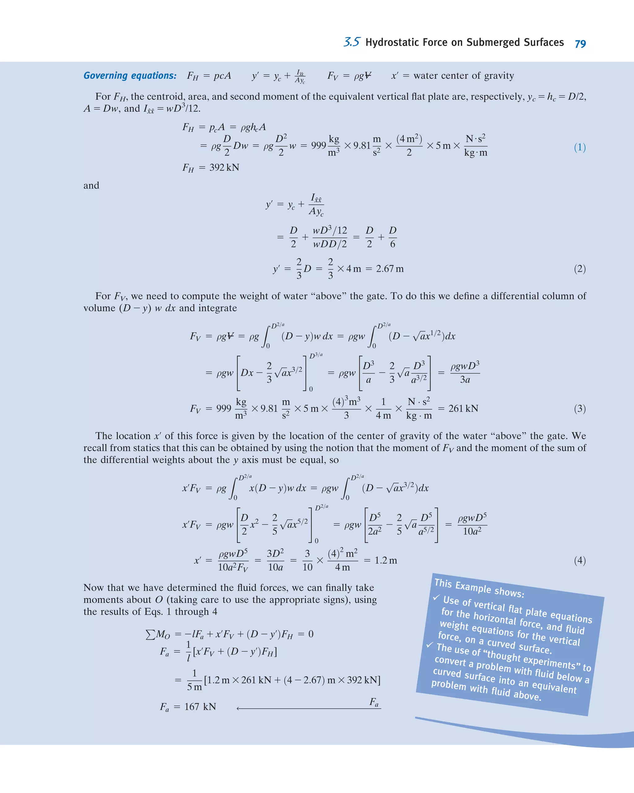
![1.6Dimensions and Units
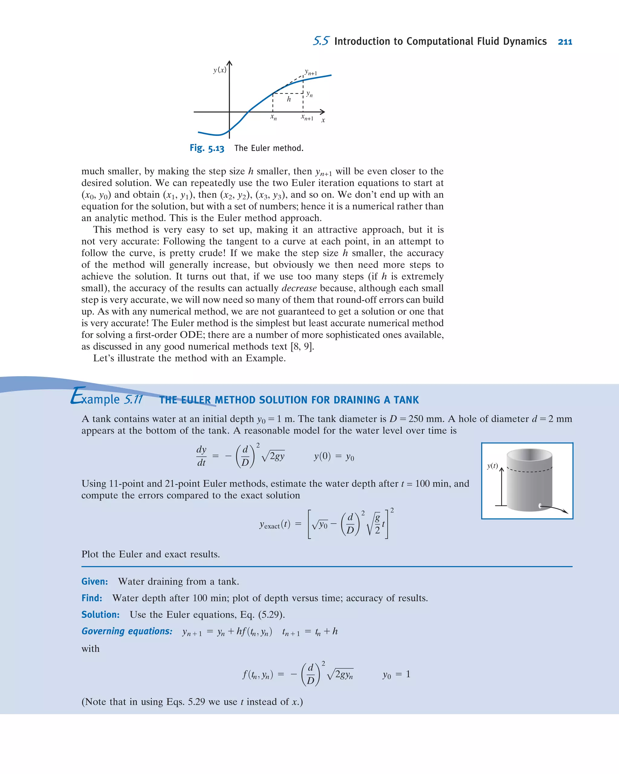
Engineering problems are solved to answer specific questions. It goes without saying
that the answer must include units. In 1999, NASA’s Mars Climate Observer crashed
because the JPL engineers assumed that a measurement was in meters, but the sup-
plying company’s engineers had actually made the measurement in feet! Conse-
quently, it is appropriate to present a brief review of dimensions and units. We say
“review” because the topic is familiar from your earlier work in mechanics.
We refer to physical quantities such as length, time, mass, and temperature as
dimensions. In terms of a particular system of dimensions, all measurable quantities
are subdivided into two groups—primary quantities and secondary quantities. We
refer to a small group of dimensions from which all others can be formed as primary
quantities, for which we set up arbitrary scales of measure. Secondary quantities are
those quantities whose dimensions are expressible in terms of the dimensions of the
primary quantities.
Units are the arbitrary names (and magnitudes) assigned to the primary dimensions
adopted as standards for measurement. For example, the primary dimension of length
may be measured in units of meters, feet, yards, or miles. These units of length are
related to each other through unit conversion factors (1 mile 5 5280 feet 5 1609 meters).
Systems of Dimensions
Any valid equation that relates physical quantities must be dimensionally homo-
geneous; each term in the equation must have the same dimensions. We recognize
that Newton’s second law (~F ~ m~a) relates the four dimensions, F, M, L, and t. Thus
force and mass cannot both be selected as primary dimensions without introducing a
constant of proportionality that has dimensions (and units).
Length and time are primary dimensions in all dimensional systems in common use.
In some systems, mass is taken as a primary dimension. In others, force is selected as a
primary dimension; a third system chooses both force and mass as primary dimen-
sions. Thus we have three basic systems of dimensions, corresponding to the different
ways of specifying the primary dimensions.
a. Mass [M], length [L], time [t], temperature [T]
b. Force [F], length [L], time [t], temperature [T]
c. Force [F], mass [M], length [L], time [t], temperature [T]
In system a, force [F] is a secondary dimension and the constant of proportionality in
Newton’s second law is dimensionless. In system b, mass [M] is a secondary dimension,
and again the constant of proportionality in Newton’s second law is dimensionless. In
system c, both force [F] and mass [M] have been selected as primary dimensions. In this
case the constant of proportionality, gc (not to be confused with g, the acceleration of
gravity!) in Newton’s second law (written ~F 5 m~a/gc) is not dimensionless. The
dimensions of gc must in fact be [ML/Ft2
] for the equation to be dimensionally
homogeneous. The numerical value of the constant of proportionality depends on the
units of measure chosen for each of the primary quantities.
Systems of Units
There is more than one way to select the unit of measure for each primary dimension.
We shall present only the more common engineering systems of units for each of the
basic systems of dimensions. Table 1.1 shows the basic units assigned to the primary
dimensions for these systems. The units in parentheses are those assigned to that unit
1.6 Dimensions and Units 11](https://image.slidesharecdn.com/foxphilipj-160402150646/75/Fox-Philip-J-Pritchard-8-ed-Mc-Donald-s-Introduction-to-Fluid-Mechanics-wiley-2011-33-2048.jpg)


![1.37 An important equation in the theory of vibrations is
m
d2
x
dt2
1 c
dx
dt
1 kx 5 fðtÞ
where m (kg) is the mass and x (m) is the position at time t (s).
For a dimensionally consistent equation, what are the
dimensions of c, k, and f? What would be suitable units for c,
k, and f in the SI and BG systems?
1.38 A parameter that is often used in describing pump
performance is the specific speed, NScu
, given by
Nscu
5
NðrpmÞ½QðgpmÞŠ1=2
½HðftÞŠ3=4
What are the units of specific speed? A particular pump has a
specific speed of 2000. What will be the specific speed in SI
units (angular velocity in rad/s)?
1.39 A particular pump has an “engineering” equation form of
the performance characteristic equation given by H (ft) 5
1.5 2 4.5 3 1025
[Q (gpm)]2
, relating the head H and flow rate
Q. What are the units of the coefficients 1.5 and 4.5 3 1025
?
Derive an SI version of this equation.
Analysis of Experimental Error
1.40 Calculate the density of standard air in a laboratory
from the ideal gas equation of state. Estimate the experi-
mental uncertainty in the air density calculated for standard
conditions (29.9 in. of mercury and 59
F) if the uncertainty in
measuring the barometer height is 60.1 in. of mercury and
the uncertainty in measuring temperature is 60.5
F. (Note
that 29.9 in. of mercury corresponds to 14.7 psia.)
1.41 Repeat the calculation of uncertainty described in Prob-
lem 1.40 for air in a hot air balloon. Assume the measured
barometer height is 759 mm of mercury with an uncertainty
of 61 mm of mercury and the temperature is 60
C with an
uncertainty of 61
C. [Note that 759 mm of mercury corre-
sponds to 101 kPa (abs).]
1.42 The mass of the standard American golf ball is 1.62 6
0.01 oz and its mean diameter is 1.68 6 0.01 in. Determine
the density and specific gravity of the American golf ball.
Estimate the uncertainties in the calculated values.
1.43 A can of pet food has the following internal dimensions:
102 mm height and 73 mm diameter (each 61 mm at odds of
20 to 1). The label lists the mass of the contents as 397 g.
Evaluate the magnitude and estimated uncertainty of the
density of the pet food if the mass value is accurate to 61 g at
the same odds.
1.44 The mass flow rate in a water flow system determined by
collecting the discharge over a timed interval is 0.2 kg/s. The
scales used can be read to the nearest 0.05 kg and the stop-
watch is accurate to 0.2 s. Estimate the precision with which
the flow rate can be calculated for time intervals of (a) 10 s
and (b) 1 min.
1.45 The mass flow rate of water in a tube is measured using a
beaker to catch water during a timed interval. The nominal
mass flow rate is 100 g/s. Assume that mass is measured using
a balance with a least count of 1 g and a maximum capacity of
1 kg, and that the timer has a least count of 0.1 s. Estimate the
time intervals and uncertainties in measured mass flow rate
that would result from using 100, 500, and 1000 mL beakers.
Would there be any advantage in using the largest beaker?
Assume the tare mass of the empty 1000 mL beaker is 500 g.
1.46 The mass of the standard British golf ball is 45.9 6 0.3 g
and its mean diameter is 41.1 6 0.3 mm. Determine the
density and specific gravity of the British golf ball. Estimate
the uncertainties in the calculated values.
1.47 The estimated dimensions of a soda can are D 5 66.0 6
0.5 mm and H 5 110 6 0.5 mm. Measure the mass of a full
can and an empty can using a kitchen scale or postal scale.
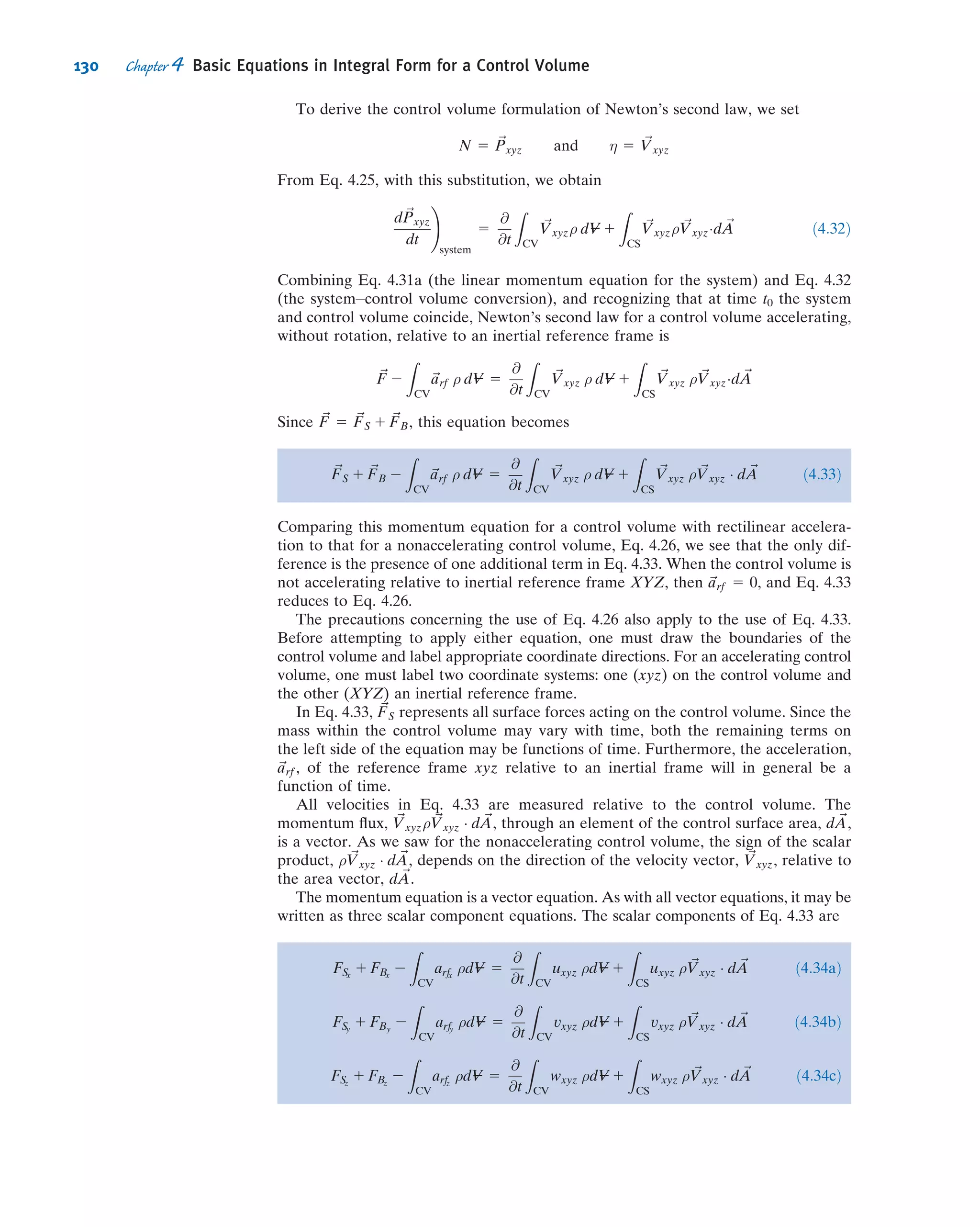
Estimate the volume of soda contained in the can. From your
measurements estimate the depth to which the can is filled
and the uncertainty in the estimate. Assume the value of
SG 5 1.055, as supplied by the bottler.
1.48 From Appendix A, the viscosity μ (N Á s/m2
) of water at
temperature T (K) can be computed from μ = A10B/(T2C)
,
where A = 2.414 3 1025
N Á s/m2
, B = 247.8 K, and C = 140 K.
Determine the viscosity of water at 30
C, and estimate its
uncertainty if the uncertainty in temperature measurement is
60.5
C.
1.49 Using the nominal dimensions of the soda can given
in Problem 1.47, determine the precision with which the
diameter and height must be measured to estimate the volume
of the can within an uncertainty of 60.5 percent.
1.50 An enthusiast magazine publishes data from its road tests
onthe lateralaccelerationcapabilityofcars.Themeasurements
are made using a 150-ft-diameter skid pad. Assume the vehicle
path deviates from the circle by 62 ft and that the vehicle speed
is read from a fifth-wheel speed-measuring system to 60.5 mph.
Estimate the experimental uncertainty in a reported lateral
acceleration of 0.7 g. How would you improve the experimental
procedure to reduce the uncertainty?
1.51 The heightofabuilding maybeestimatedbymeasuringthe
horizontal distance to a point on the ground and the angle from
this point to the top of the building. Assuming these measure-
mentsare L 5 1006 0.5ftandθ 5 306 0.2
, estimatethe height
H of the building and the uncertainty in the estimate. For the
same building height and measurement uncertainties, use
Excel’s Solver to determine the angle (and the corresponding
distance from the building) at which measurements should be
made tominimize the uncertaintyin estimated height. Evaluate
and plot the optimum measurement angle as a function of
building height for 50 # H # 1000 ft.
1.52 An American golf ball is described in Problem 1.42
Assuming the measured mass and its uncertainty as given,
determine the precision to which the diameter of the ball
must be measured so the density of the ball may be estimated
within an uncertainty of 61 percent.
1.53 A syringe pump is to dispense liquid at a flow rate of
100 mL/min. The design for the piston drive is such that the
uncertainty of the piston speed is 0.001 in./min, and the
cylinder bore diameter has a maximum uncertainty of 0.0005
in. Plot the uncertainty in the flow rate as a function of
cylinder bore. Find the combination of piston speed and bore
that minimizes the uncertainty in the flow rate.
Problems 19](https://image.slidesharecdn.com/foxphilipj-160402150646/75/Fox-Philip-J-Pritchard-8-ed-Mc-Donald-s-Introduction-to-Fluid-Mechanics-wiley-2011-41-2048.jpg)


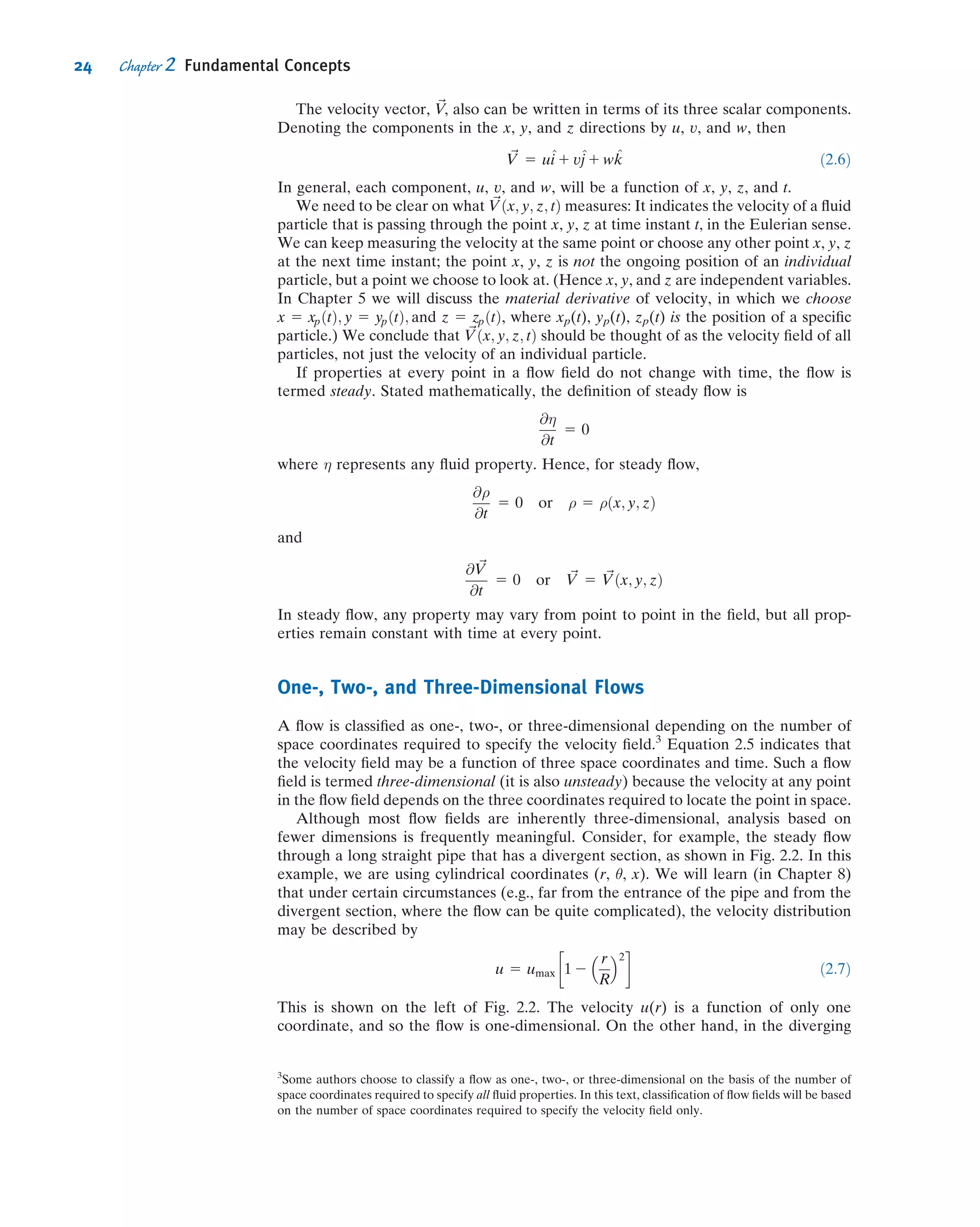
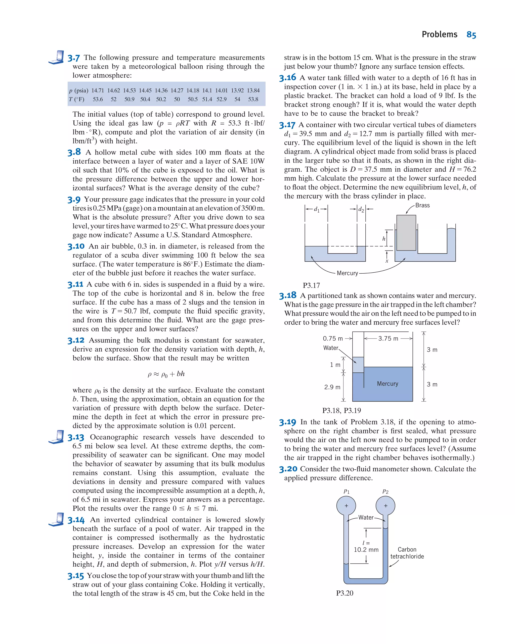
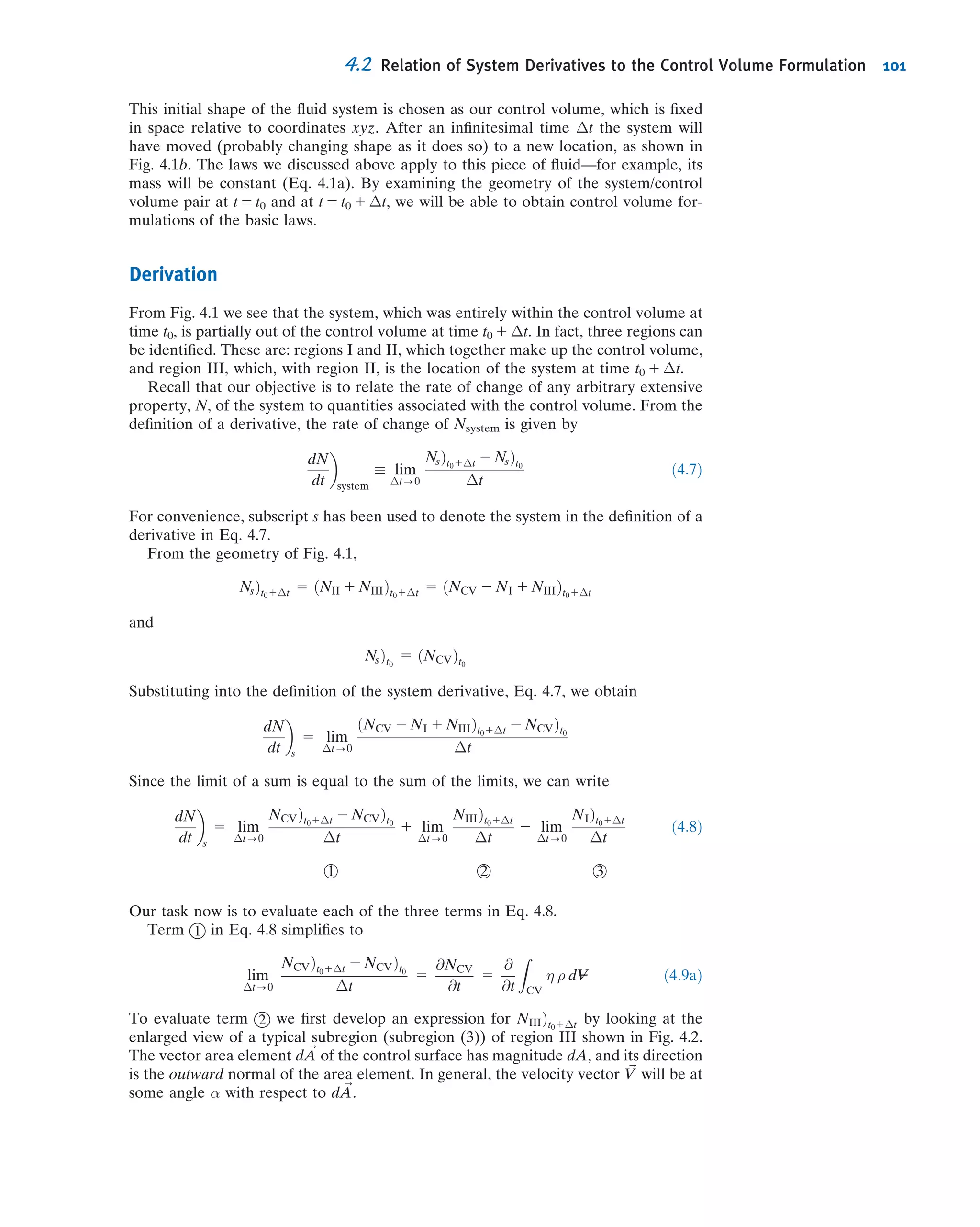
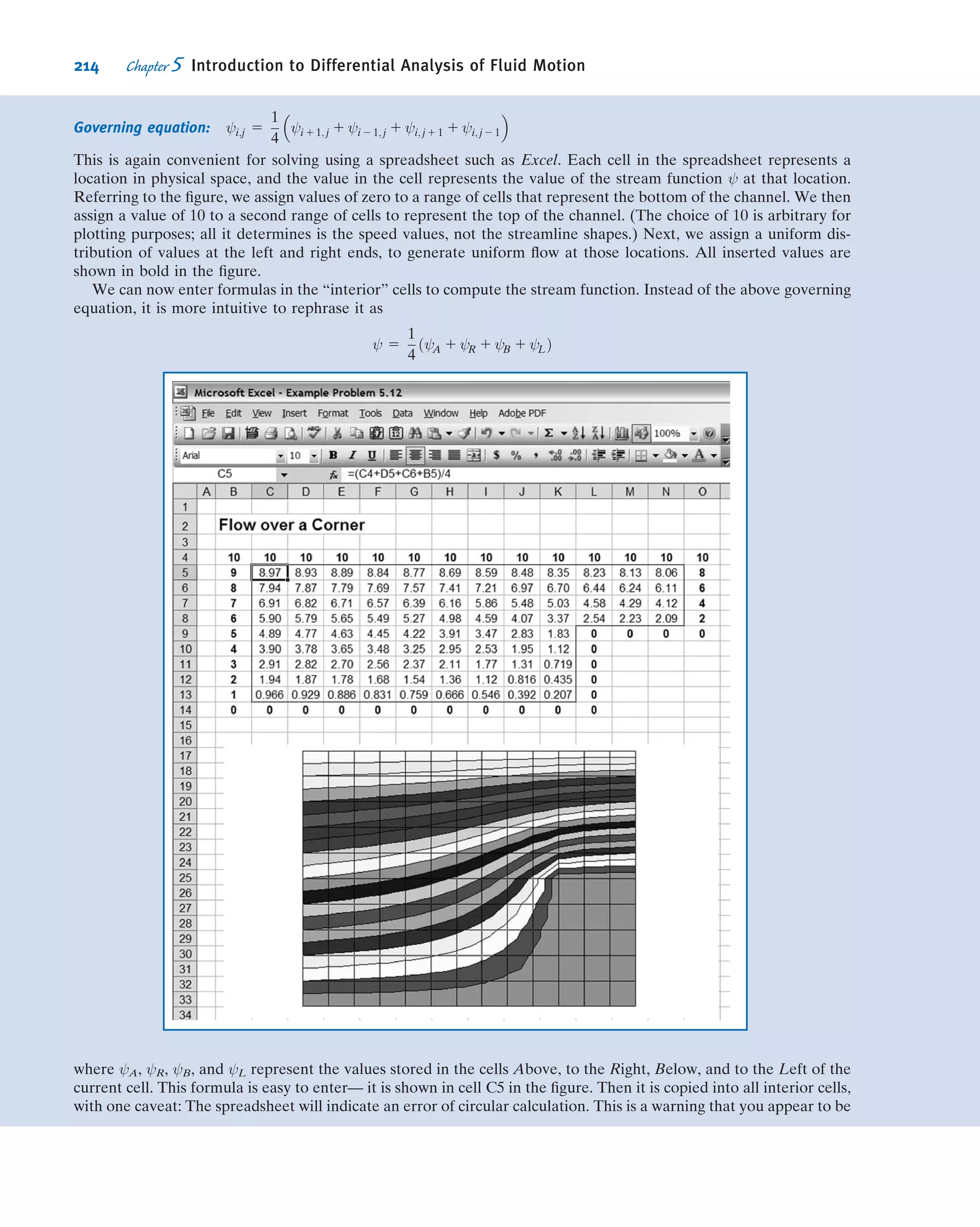
![specialized equipment, we are not aware of the underlying molecular nature of fluids.
This molecular structure is one in which the mass is not continuously distributed in
space, but is concentrated in molecules that are separated by relatively large regions
of empty space. The sketch in Fig. 2.1a shows a schematic representation of this. A
region of space “filled” by a stationary fluid (e.g., air, treated as a single gas) looks like
a continuous medium, but if we zoom in on a very small cube of it, we can see that we
mostly have empty space, with gas molecules scattered around, moving at high speed
(indicated by the gas temperature). Note that the size of the gas molecules is greatly
exaggerated (they would be almost invisible even at this scale) and that we have
placed velocity vectors only on a small sample. We wish to ask: What is the minimum
volume, δV---u, that a “point” C must be, so that we can talk about continuous fluid
properties such as the density at a point? In other words, under what circumstances
can a fluid be treated as a continuum, for which, by definition, properties vary
smoothly from point to point? This is an important question because the concept of a
continuum is the basis of classical fluid mechanics.
Consider how we determine the density at a point. Density is defined as mass per
unit volume; in Fig. 2.1a the mass δm will be given by the instantaneous number of
molecules in δV--- (and the mass of each molecule), so the average density in volume δV---
is given by ρ 5 δm=δV---. We say “average” because the number of molecules in δV---,
and hence the density, fluctuates. For example, if the gas in Fig. 2.1a was air at
standard temperature and pressure (STP1
) and the volume δV--- was a sphere of dia-
meter 0.01 μm, there might be 15 molecules in δV--- (as shown), but an instant later
there might be 17 (three might enter while one leaves). Hence the density at “point” C
randomly fluctuates in time, as shown in Fig. 2.1b. In this figure, each vertical dashed
line represents a specific chosen volume, δV---, and each data point represents the
measured density at an instant. For very small volumes, the density varies greatly, but
above a certain volume, δV---u, the density becomes stable—the volume now encloses a
huge number of molecules. For example, if δV--- 5 0:001 mm3
(about the size of a grain
of sand), there will on average be 2:5 3 1013
molecules present. Hence we can con-
clude that air at STP (and other gases, and liquids) can be treated as a continuous
medium as long as we consider a “point” to be no smaller than about this size; this is
sufficiently precise for most engineering applications.
The concept of a continuum is the basis of classical fluid mechanics. The con-
tinuum assumption is valid in treating the behavior of fluids under normal conditions.
It only breaks down when the mean free path of the molecules2
becomes the same
order of magnitude as the smallest significant characteristic dimension of the problem.
(a) (b)
C
x
y
“Point” C at x,y,z
Volume
of mass
δV
δm
δm/δV
δV δV'
Fig. 2.1 Definition of density at a point.
VIDEO
Fluid as a Continuum.
1
STP for air are 15
C (59
F) and 101.3 kPa absolute (14.696 psia), respectively.
2
Approximately 6 3 1028
m at STP (Standard Temperature and Pressure) for gas molecules that show ideal
gas behavior [1].
22 Chapter 2 Fundamental Concepts](https://image.slidesharecdn.com/foxphilipj-160402150646/75/Fox-Philip-J-Pritchard-8-ed-Mc-Donald-s-Introduction-to-Fluid-Mechanics-wiley-2011-44-2048.jpg)
![section, the velocity decreases in the x direction, and the flow becomes two-dimensional:
u 5 u(r, x).
As you might suspect, the complexity of analysis increases considerably with the
number of dimensions of the flow field. For many problems encountered in engi-
neering, a one-dimensional analysis is adequate to provide approximate solutions of
engineering accuracy.
Since all fluids satisfying the continuum assumption must have zero relative velocity
at a solid surface (to satisfy the no-slip condition), most flows are inherently two-
or three-dimensional. To simplify the analysis it is often convenient to use the notion
of uniform flow at a given cross section. In a flow that is uniform at a given cross
section, the velocity is constant across any section normal to the flow. Under this
assumption,4
the two-dimensional flow of Fig. 2.2 is modeled as the flow shown in
Fig. 2.3. In the flow of Fig. 2.3, the velocity field is a function of x alone, and thus the
flow model is one-dimensional. (Other properties, such as density or pressure, also
may be assumed uniform at a section, if appropriate.)
The term uniform flow field (as opposed to uniform flow at a cross section) is used
to describe a flow in which the velocity is constant, i.e., independent of all space
coordinates, throughout the entire flow field.
Timelines, Pathlines, Streaklines, and Streamlines
Airplane and auto companies and college engineering laboratories, among others,
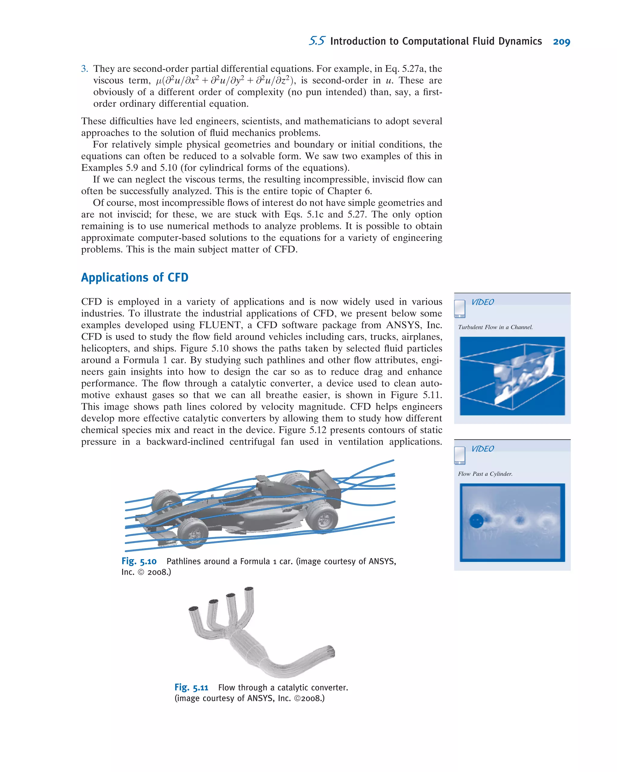
frequently use wind tunnels to visualize flow fields [2]. For example, Fig. 2.4 shows a
flow pattern for flow around a car mounted in a wind tunnel, generated by releasing
smoke into the flow at five fixed upstream points. Flow patterns can be visualized
using timelines, pathlines, streaklines, or streamlines.
If a number of adjacent fluid particles in a flow field are marked at a given instant, they
form a line in the fluid at that instant; this line is called a timeline. Subsequent observa-
tions of the line may provide information about the flow field. For example, in discussing
the behavior of a fluid under the action of a constant shear force (Section 1.2) timelines
were introduced to demonstrate the deformation of a fluid at successive instants.
A pathline is the path or trajectory traced out by a moving fluid particle. To make a
pathline visible, we might identify a fluid particle at a given instant, e.g., by the use of
dye or smoke, and then take a long exposure photograph of its subsequent motion.
The line traced out by the particle is a pathline. This approach might be used to study,
for example, the trajectory of a contaminant leaving a smokestack.
On the other hand, we might choose to focus our attention on a fixed location in
space and identify, again by the use of dye or smoke, all fluid particles passing through
this point. After a short period of time we would have a number of identifiable fluid
u(r)
r
x
R
r
θ
u(r,x)
umax
Fig. 2.2 Examples of one- and two-dimensional flows.
x
Fig. 2.3 Example of uniform
flow at a section.
4
This may seem like an unrealistic simplification, but actually in many cases leads to useful results. Sweeping
assumptions such as uniform flow at a cross section should always be reviewed carefully to be sure they
provide a reasonable analytical model of the real flow.
CLASSIC VIDEO
Flow Visualization.
VIDEO
Streaklines.
2.2 Velocity Field 25](https://image.slidesharecdn.com/foxphilipj-160402150646/75/Fox-Philip-J-Pritchard-8-ed-Mc-Donald-s-Introduction-to-Fluid-Mechanics-wiley-2011-47-2048.jpg)


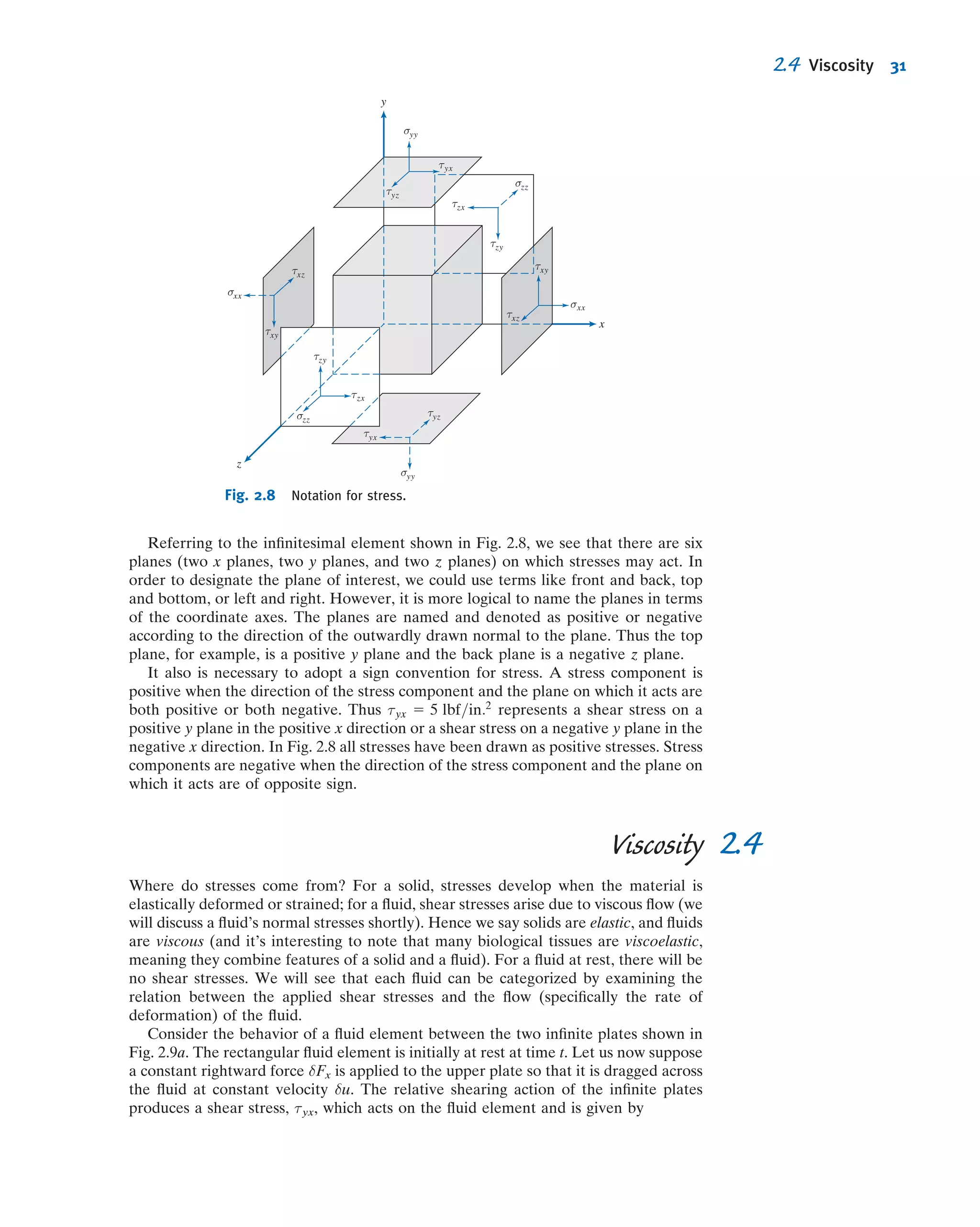

![proportionality in Eq. 2.14 is the absolute (or dynamic) viscosity, μ. Thus in terms of the
coordinates of Fig. 2.9, Newton’s law of viscosity is given for one-dimensional flow by
τyx 5 μ
du
dy
ð2:15Þ
Note that, since the dimensions of τ are [F/L2
] and the dimensions of du/dy are [1/t], μ has
dimensions [Ft/L2
]. Since the dimensions of force, F, mass, M, length, L, and time, t, are
related by Newton’s second law of motion, the dimensions of μ can also be expressed
as [M/Lt]. In the British Gravitational system, the units of viscosity are lbf Á s/ft2
or slug/
(ft Á s). In the Absolute Metric system, the basic unit of viscosity is called a poise [1 poise
1 g/(cm Á s)]; in the SI system the units of viscosity are kg/(m Á s) or Pa Á s (1 PaÁ s 5
1 N Á s/m2
). The calculation of viscous shear stress is illustrated in Example 2.2.
In fluid mechanics the ratio of absolute viscosity, μ, to density, ρ, often arises. This
ratio is given the name kinematic viscosity and is represented by the symbol ν. Since
density has dimensions [M/L3
], the dimensions of ν are [L2
/t]. In the Absolute Metric
system of units, the unit for ν is a stoke (1 stoke 1 cm2
/s).
Viscosity data for a number of common Newtonian fluids are given in Appendix A.
Note that for gases, viscosity increases with temperature, whereas for liquids, viscosity
decreases with increasing temperature.
Example 2.2 VISCOSITY AND SHEAR STRESS IN NEWTONIAN FLUID
An infinite plate is moved over a second plate on a layer of liquid as shown. For small gap width, d, we assume a
linear velocity distribution in the liquid. The liquid viscosity is 0.65 centipoise and its specific gravity is 0.88.
Determine:
(a) The absolute viscosity of the liquid, in lbf Á s/ft2
.
(b) The kinematic viscosity of the liquid, in m2
/s.
(c) The shear stress on the upper plate, in lbf/ft2
.
(d) The shear stress on the lower plate, in Pa.
(e) The direction of each shear stress calculated in parts (c) and (d).
Given: Linear velocity profile in the liquid between infinite parallel
plates as shown.
μ 5 0:65 cp
SG 5 0:88
Find: (a) μ in units of lbf Á s/ft2
.
(b) ν in units of m2
/s.
(c) τ on upper plate in units of lbf/ft2
.
(d) τ on lower plate in units of Pa.
(e) Direction of stresses in parts (c) and (d).
Solution:
Governing equation: τyx 5 μ
du
dy
Definition: ν 5
μ
ρ
Assumptions: (1) Linear velocity distribution (given)
(2) Steady flow
(3) μ 5 constant
(a) μ 5 0:65 cp 3
poise
100 cp
3
g
cmÁsÁpoise
3
lbm
454 g
3
slug
32:2 lbm
3 30:5
cm
ft
3
lbf Á s2
slug Á ft
μ 5 1:36 3 1025
lbf Á s=ft2
ß
μ
x
y
U = 0.3 m/s
d = 0.3 mm
x
y
U = 0.3 m/s
d = 0.3 mm
2.4 Viscosity 33](https://image.slidesharecdn.com/foxphilipj-160402150646/75/Fox-Philip-J-Pritchard-8-ed-Mc-Donald-s-Introduction-to-Fluid-Mechanics-wiley-2011-55-2048.jpg)
![Non-Newtonian Fluids
Fluids in which shear stress is not directly proportional to deformation rate are non-
Newtonian. Although we will not discuss these much in this text, many common fluids
exhibit non-Newtonian behavior. Two familiar examples are toothpaste and Lucite5
paint. The latter is very “thick” when in the can, but becomes “thin” when sheared by
brushing. Toothpaste behaves as a “fluid” when squeezed from the tube. However, it
does not run out by itself when the cap is removed. There is a threshold or yield stress
below which toothpaste behaves as a solid. Strictly speaking, our definition of a fluid is
valid only for materials that have zero yield stress. Non-Newtonian fluids commonly
are classified as having time-independent or time-dependent behavior. Examples of
time-independent behavior are shown in the rheological diagram of Fig. 2.10.
Numerous empirical equations have been proposed [3, 4] to model the observed
relations between τyx and du/dy for time-independent fluids. They may be adequately
(b) ν 5
μ
ρ
5
μ
SG ρH2O
5 1:36 3 1025 lbf Á s
ft2
3
ft3
ð0:88Þ1:94 slug
3
slug Á ft
lbf Á s2
3 ð0:305Þ2 m2
ft2
ν 5 7:41 3 1027
m2
=s ß
ν
(c) τupper 5 τyx; upper 5 μ
du
dy
y5d
Since u varies linearly with y,
du
dy
5
Δu
Δy
5
U 2 0
d 2 0
5
U
d
5 0:3
m
s
3
1
0:3 mm
3 1000
mm
m
5 1000 s21
τupper 5 μ
U
d
5 1:36 3 1025 lbf Á s
ft2
3
1000
s
5 0:0136 lbf=ft2
ß
τupper
(d) τlower 5 μ
U
d
5 0:0136
lbf
ft2
3 4:45
N
lbf
3
ft2
ð0:305Þ2
m2
3
Pa Á m2
N
5 0:651 Pa ß
τlower
(e) Directions of shear stresses on upper and lower plates.
The upper plate is a negative y surface; so
positive τyx acts in the negative x direction:
The lower plate is a positive y surface; so
positive τyx acts in the positive x direction:
ß
ðeÞx
y
τupper
τlower
Part (c) shows that the shear stress
is:
ü Constant across the gap for a lin-
ear velocity profile.ü Directly proportional to the speed
of the upper plate (because of the
linearity of Newtonian fluids).
ü Inversely proportional to the gap
between the plates.Note that multiplying the shear stress
by the plate area in such problems
computes the force required to
maintain the motion.
5
Trademark, E. I. du Pont de Nemours Company.
34 Chapter 2 Fundamental Concepts](https://image.slidesharecdn.com/foxphilipj-160402150646/75/Fox-Philip-J-Pritchard-8-ed-Mc-Donald-s-Introduction-to-Fluid-Mechanics-wiley-2011-56-2048.jpg)

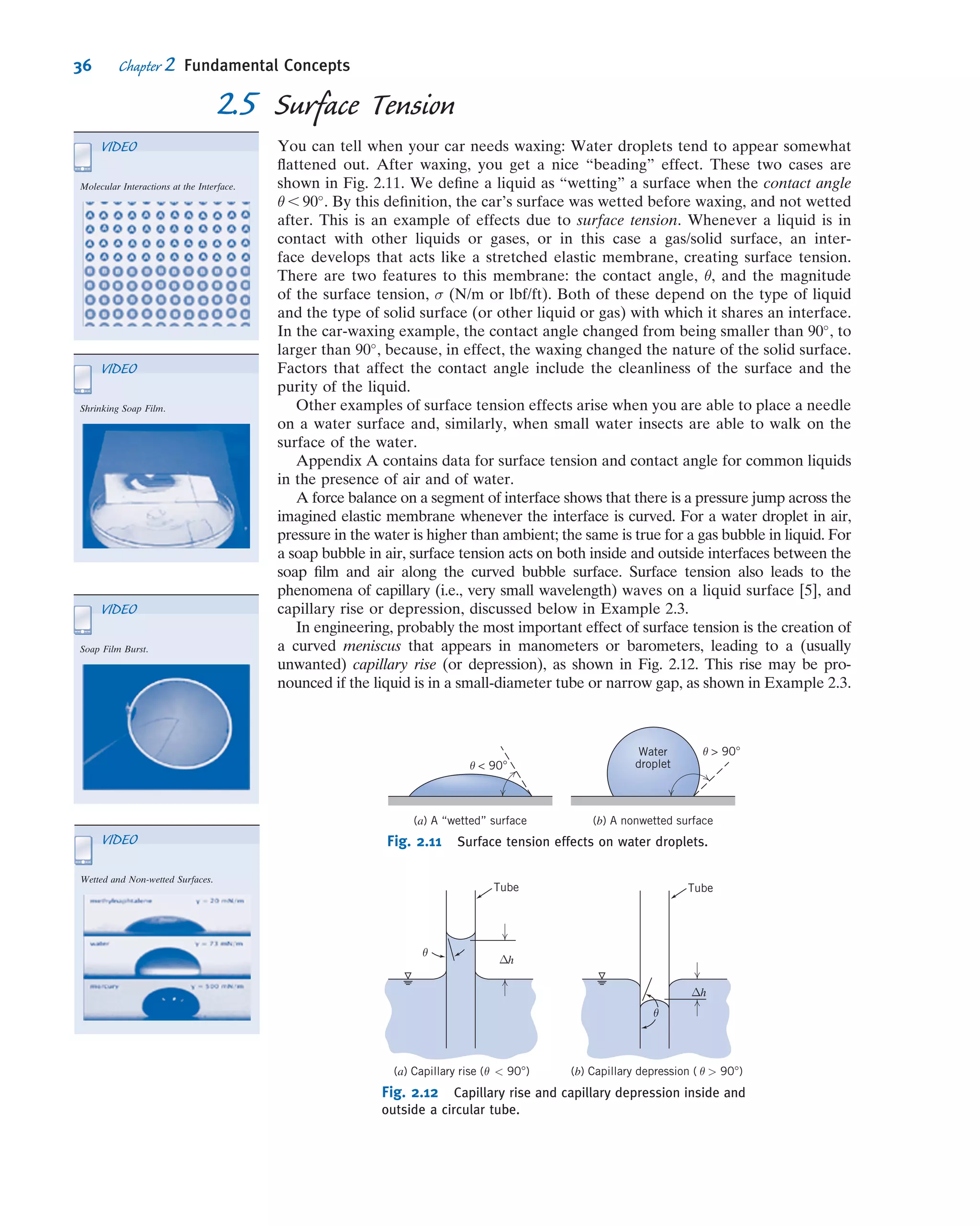


![2.5 Surface Tension
You can tell when your car needs waxing: Water droplets tend to appear somewhat
flattened out. After waxing, you get a nice “beading” effect. These two cases are
shown in Fig. 2.11. We define a liquid as “wetting” a surface when the contact angle
θ , 90
. By this definition, the car’s surface was wetted before waxing, and not wetted
after. This is an example of effects due to surface tension. Whenever a liquid is in
contact with other liquids or gases, or in this case a gas/solid surface, an inter-
face develops that acts like a stretched elastic membrane, creating surface tension.
There are two features to this membrane: the contact angle, θ, and the magnitude
of the surface tension, σ (N/m or lbf/ft). Both of these depend on the type of liquid
and the type of solid surface (or other liquid or gas) with which it shares an interface.
In the car-waxing example, the contact angle changed from being smaller than 90
, to
larger than 90
, because, in effect, the waxing changed the nature of the solid surface.
Factors that affect the contact angle include the cleanliness of the surface and the
purity of the liquid.
Other examples of surface tension effects arise when you are able to place a needle
on a water surface and, similarly, when small water insects are able to walk on the
surface of the water.
Appendix A contains data for surface tension and contact angle for common liquids
in the presence of air and of water.
A force balance on a segment of interface shows that there is a pressure jump across the
imagined elastic membrane whenever the interface is curved. For a water droplet in air,
pressure in the water is higher than ambient; the same is true for a gas bubble in liquid. For
a soap bubble in air, surface tension acts on both inside and outside interfaces between the
soap film and air along the curved bubble surface. Surface tension also leads to the
phenomena of capillary (i.e., very small wavelength) waves on a liquid surface [5], and
capillary rise or depression, discussed below in Example 2.3.
In engineering, probably the most important effect of surface tension is the creation of
a curved meniscus that appears in manometers or barometers, leading to a (usually
unwanted) capillary rise (or depression), as shown in Fig. 2.12. This rise may be pro-
nounced if the liquid is in a small-diameter tube or narrow gap, as shown in Example 2.3.
(a) A “wetted” surface
θ 90°
(b) A nonwetted surface
Water
droplet
θ 90°
Fig. 2.11 Surface tension effects on water droplets.
Tube Tube
h
h
θ
θ
θ(a) Capillary rise ( 90°) (b) Capillary depression ( 90°)θ
Δ
Δ
Fig. 2.12 Capillary rise and capillary depression inside and
outside a circular tube.
VIDEO
Molecular Interactions at the Interface.
VIDEO
Shrinking Soap Film.
VIDEO
Soap Film Burst.
VIDEO
Wetted and Non-wetted Surfaces.
36 Chapter 2 Fundamental Concepts](https://image.slidesharecdn.com/foxphilipj-160402150646/75/Fox-Philip-J-Pritchard-8-ed-Mc-Donald-s-Introduction-to-Fluid-Mechanics-wiley-2011-66-2048.jpg)
![Folsom [6] shows that the simple analysis of Example 2.3 overpredicts the capillary
effect and gives reasonable results only for tube diameters less than 0.1 in. (2.54 mm).
Over a diameter range 0.1 , D , 1.1 in., experimental data for the capillary rise with a
water-air interface are correlated by the empirical expression Δh 5 0.400/e4.37D
.
Manometer and barometer readings should be made at the level of the middle of
the meniscus. This is away from the maximum effects of surface tension and thus
nearest to the proper liquid level.
All surface tension data in Appendix A were measured for pure liquids in contact
with clean vertical surfaces. Impurities in the liquid, dirt on the surface, or surface
inclination can cause an indistinct meniscus; under such conditions it may be difficult
to determine liquid level accurately. Liquid level is most distinct in a vertical tube.
When inclined tubes are used to increase manometer sensitivity (see Section 3.3) it is
important to make each reading at the same point on the meniscus and to avoid use of
tubes inclined less than about 15
from horizontal.
Surfactant compounds reduce surface tension significantly (more than 40% with
little change in other properties [7]) when added to water. They have wide commercial
application: Most detergents contain surfactants to help water penetrate and lift soil
from surfaces. Surfactants also have major industrial applications in catalysis, aero-
sols, and oil field recovery.
2.6 Description and Classification of Fluid Motions
In Chapter 1 and in this chapter, we have almost completed our brief introduction to
some concepts and ideas that are often needed when studying fluid mechanics. Before
beginning detailed analysis of fluid mechanics in the rest of this text, we will describe some
interesting examples to illustrate a broad classification of fluid mechanics on the basis of
important flow characteristics. Fluid mechanics is a huge discipline: It covers everything
from the aerodynamics of a supersonic transport vehicle to the lubrication of human joints
by sinovial fluid. We need to break fluid mechanics down into manageable proportions. It
turns out that the two most difficult aspects of a fluid mechanics analysis to deal with are:
(1) the fluid’s viscous nature and (2) its compressibility. In fact, the area of fluid mechanics
theory that first became highly developed (about 250 years ago!) was that dealing with a
frictionless, incompressible fluid. As we will see shortly (and in more detail later on), this
theory, while extremely elegant, led to the famous result called d’Alembert’s paradox: All
bodies experience no drag as they move through such a fluid—a result not exactly con-
sistent with any real behavior!
Although not the only way to do so, most engineers subdivide fluid mechanics in
terms of whether or not viscous effects and compressibility effects are present, as
shown in Fig. 2.13. Also shown are classifications in terms of whether a flow is laminar
or turbulent, and internal or external. We will now discuss each of these.
Viscous and Inviscid Flows
When you send a ball flying through the air (as in a game of baseball, soccer, or any
number of other sports), in addition to gravity the ball experiences the aerodynamic
drag of the air. The question arises: What is the nature of the drag force of the air on
the ball? At first glance, we might conclude that it’s due to friction of the air as it flows
over the ball; a little more reflection might lead to the conclusion that because air has
such a low viscosity, friction might not contribute much to the drag, and the drag
might be due to the pressure build-up in front of the ball as it pushes the air out of the
way. The question arises: Can we predict ahead of time the relative importance of
the viscous force, and force due to the pressure build-up in front of the ball? Can we
make similar predictions for any object, for example, an automobile, a submarine, a
VIDEO
Capillary Rise.
CLASSIC VIDEO
Surface Tension in Fluid Mechanics.
VIDEO
Examples of Flow over a Sphere.
38 Chapter 2 Fundamental Concepts](https://image.slidesharecdn.com/foxphilipj-160402150646/75/Fox-Philip-J-Pritchard-8-ed-Mc-Donald-s-Introduction-to-Fluid-Mechanics-wiley-2011-68-2048.jpg)


![References
1. Vincenti, W. G., and C. H. Kruger Jr., Introduction to
Physical Gas Dynamics. New York: Wiley, 1965.
2. Merzkirch, W., Flow Visualization, 2nd ed. New York:
Academic Press, 1987.
3. Tanner, R. I., Engineering Rheology. Oxford: Clarendon
Press, 1985.
4. Macosko, C. W., Rheology: Principles, Measurements, and
Applications. New York: VCH Publishers, 1994.
5. Loh, W. H. T., “Theory of the Hydraulic Analogy for
Steady and Unsteady Gas Dynamics,” in Modern Develop-
ments in Gas Dynamics, W. H. T. Loh, ed. New York: Plenum,
1969.
6. Folsom, R. G., “Manometer Errors Due to Capillarity,”
Instruments, 9, 1, 1937, pp. 36À37.
7. Waugh, J. G., and G. W. Stubstad, Hydroballistics Model-
ing. San Diego: Naval Undersea Center, ca. 1972.
Problems
Velocity Field
2.1 For the velocity fields given below, determine:
a. whether the flow field is one-, two-, or three-dimensional,
and why.
b. whether the flow is steady or unsteady, and why.
(The quantities a and b are constants.)
(1) ~V ¼ ½ðax þ tÞeby
Š^i (2) ~V ¼ ðax 2 byÞ^i
(3) ~V ¼ ax^i þ ½ebx
Š^j (4) ~V ¼ ax^i þ bx2 ^j þ ax ^k
(5) ~V ¼ ax^i þ ½ebt
Š^j (6) ~V ¼ ax^i þ bx2 ^j þ ay ^k
(7) ~V ¼ ax^i þ ½ebt
Š^j þ ay ^k (8) ~V ¼ ax^i þ ½eby
Š^j þ az ^k
2.2 For the velocity fields given below, determine:
a. whether the flow field is one-, two-, or three-dimensional,
and why.
b. whether the flow is steady or unsteady, and why.
(The quantities a and b are constants.)
(1) ~V 5 [ay2
e2bt
]^i (2) ~V 5 ax2^i 1 bx^j 1 c ^k
(3) ~V 5 axy^i 2 byt^j (4) ~V 5 ax^i 2 by^j 1 ct ^k
(5) ~V 5 [ae2bx
]^i 1 bt2^j (6) ~V 5 aðx2
1 y2
Þ1=2
ð1=z3
Þ ^k
(7) ~V 5 ðax 1 tÞ^i 2 by2^j (8) ~V 5 ax2^i 1 bxz^j 1 cy ^k
2.3 A viscous liquid is sheared between two parallel disks; the
upper disk rotates and the lower one is fixed. The velocity
field between the disks is given by ~V 5 ^eθrωz=h. (The origin
of coordinates is located at the center of the lower disk; the
upper disk is located at z 5 h.) What are the dimensions of
this velocity field? Does this velocity field satisfy appropriate
physical boundary conditions? What are they?
2.4 For the velocity field ~V ¼ Ax2
y^i þ Bxy2^j, where
A 5 2 m22
s21
and B 5 1 m22
s21
, and the coordinates are
measured in meters, obtain an equation for the flow
streamlines. Plot several streamlines in the first quadrant.
2.5 The velocity field ~V ¼ Ax^i 2 Ay^j, where A 5 2 s21
, can be
interpreted to represent flow in a corner. Find an equation
for the flow streamlines. Explain the relevance of A. Plot
several streamlines in the first quadrant, including the one
that passes through the point (x, y) 5 (0, 0).
2.6 A velocity field is specified as ~V 5 axy^i 1 by2^j, where
a 5 2 m21
s21
, b 5 26 m21
s21
, and the coordinates are mea-
sured in meters. Is the flow field one-, two-, or three-
dimensional? Why? Calculate the velocity components at the
point (2, 1
/2). Develop an equation for the streamline passing
through this point. Plot several streamlines in the first quad-
rant including the one that passes through the point (2, 1
/2).
2.7 A velocity field is given by ~V 5 ax^i 2 bty^j, where a 5 1 s21
and b 5 1 s22
. Find the equation of the streamlines at any
time t. Plot several streamlines in the first quadrant at t 5 0 s,
t 5 1 s, and t 5 20 s.
2.8 A velocity field is given by ~V 5 ax3^i 1 bxy3^j, where
a 5 1 m22
s21
and b 5 1 m23
s21
. Find the equation of the
streamlines. Plot several streamlines in the first quadrant.
2.9 A flow is described by the velocity field ~V 5 ðAx 1 BÞ^i 1
ð2AyÞ^j, where A 5 10 ft/s/ft and B 5 20 ft/s. Plot a few
streamlines in the xy plane, including the one that passes
through the point (x, y) 5 (1, 2).
2.10 The velocity for a steady, incompressible flow in the xy
plane is given by ~V 5 ^iA=x 1 ^jAy=x2
, where A 5 2 m2
/s, and
the coordinates are measured in meters. Obtain an equation
for the streamline that passes through the point (x, y) 5
(1, 3). Calculate the time required for a fluid particle to move
from x 5 1 m to x 5 2 m in this flow field.
2.11 The flow field for an atmospheric flow is given by
~V ¼ 2
My
2π
^i þ
Mx
2π
^j
where M 5 1 s21
, and the x and y coordinates are the parallel
to the local latitude and longitude. Plot the velocity
magnitude along the x axis, along the y axis, and along the
line y 5 x, and discuss the velocity direction with respect to
these three axes. For each plot use a range x or y 5 0 km
to 1 km. Find the equation for the streamlines and sketch
several of them. What does this flow field model?
2.12 The flow field for an atmospheric flow is given by
~V ¼ 2
Ky
2πðx2 þ y2Þ
^i þ
Kx
2πðx2 þ y2Þ
^j
where K 5 105
m2
/s, and the x and y coordinates are parallel to
the local latitude and longitude. Plot the velocity magnitude
along the x axis, along the y axis, and along the line y 5 x, and
discuss the velocity direction with respect to these three axes.
For each plot use a range x or y 5 2 1 km to 1 km, excluding |x|
or |y| , 100 m. Find the equation for the streamlines and
sketch several of them. What does this flow field model?
2.13 A flow field is given by
~V ¼ 2
qx
2πðx2 þ y2Þ
^i 2
qy
2πðx2 þ y2Þ
^j
46 Chapter 2 Fundamental Concepts](https://image.slidesharecdn.com/foxphilipj-160402150646/75/Fox-Philip-J-Pritchard-8-ed-Mc-Donald-s-Introduction-to-Fluid-Mechanics-wiley-2011-82-2048.jpg)
![where q 5 5 3 104
m2
/s. Plot the velocity magnitude along
the x axis, along the y axis, and along the line y 5 x, and
discuss the velocity direction with respect to these three axes.
For each plot use a range x or y = 2 1 km to 1 km, excluding
jxj or jyj , 100 m. Find the equation for the streamlines and
sketch several of them. What does this flow field model?
2.14 Beginning with the velocity field of Problem 2.5, show
that the parametric equations for particle motion are given
by xp ¼ c1eAt
and yp ¼ c2e2 At
. Obtain the equation for the
pathline of the particle located at the point (x, y) 5 (2, 2) at
the instant t 5 0. Compare this pathline with the streamline
through the same point.
2.15 A flow field is given by ~V ¼ Ax^i þ 2Ay^j, where A 5 2 s21
.
Verify that the parametric equations for particle motion are
given by xp 5 c1eAt
and yp 5 c2e2At
. Obtain the equation for the
pathline of the particle located at the point (x, y) 5 (2, 2) at the
instant t 5 0. Compare this pathline with the streamline
through the same point.
2.16 A velocity field is given by ~V 5 ayt^i 2 bx^j, where a 5 1 s22
and b 5 4 s21
. Find the equation of the streamlines at any time t.
Plot several streamlines at t 5 0 s, t 5 1 s, and t 5 20 s.
2.17 Verify that xp 5 2asin(ωt), yp 5 acos(ωt) is the equation
for the pathlines of particles for the flow field of Problem
2.12. Find the frequency of motion ω as a function of the
amplitude of motion, a, and K. Verify that xp 5 2asin(ωt),
yp 5 acos(ωt) is also the equation for the pathlines of parti-
cles for the flow field of Problem 2.11, except that ω is now a
function of M. Plot typical pathlines for both flow fields and
discuss the difference.
2.18 Air flows downward toward an infinitely wide horizontal
flat plate. The velocity field is given by ~V 5 ðax^i 2 ay^jÞð2 1
cos ωtÞ, where a 5 5 s21
, ω 5 2π s21
, x and y (measured in
meters) are horizontal and vertically upward, respectively, and t
is in s. Obtain an algebraic equation for a streamline at t5 0.
Plot the streamline that passes through point (x, y) 5 (3, 3) at
this instant. Will the streamline change with time? Explain
briefly. Show the velocity vector on your plot at the same point
and time. Is the velocity vector tangent to the streamline?
Explain.
2.19 Consider the flow described by the velocity field
~V ¼ Að1 þ BtÞ^i þ Cty^j, with A 5 1 m/s, B 5 1 s21
, and C 5 1
s22
. Coordinates are measured in meters. Plot the pathline
traced out by the particle that passes through the point (1, 1) at
time t 5 0. Compare with the streamlines plotted through the
same point at the instants t 5 0, 1, and 2 s.
2.20 Consider the flow described by the velocity field
~V 5 Bxð1 1 AtÞ^i 1 Cy^j, with A 5 0.5 s21
and B 5 C 5 1 s21
.
Coordinates are measured in meters. Plot the pathline traced
out by the particle that passes through the point (1, 1) at time
t 5 0. Compare with the streamlines plotted through the
same point at the instants t 5 0, 1, and 2 s.
2.21 Consider the flow field given in Eulerian description by
the expression ~V ¼ A^i 2 Bt^j, where A 5 2 m/s, B 5 2 m/s2
,
and the coordinates are measured in meters. Derive the
Lagrangian position functions for the fluid particle that was
located at the point (x, y) 5 (1, 1) at the instant t 5 0. Obtain
an algebraic expression for the pathline followed by this
particle. Plot the pathline and compare with the stream-
lines plotted through the same point at the instants t 5 0, 1,
and 2 s.
2.22 Consider the velocity field V 5 ax^i 1 byð1 1 ctÞ^j, where
a 5 b 5 2 s21
and c 5 0.4 s21
. Coordinates are measured in
meters. For the particle that passes through the point
(x, y) 5 (1, 1) at the instant t 5 0, plot the pathline during the
interval from t 5 0 to 1.5 s. Compare this pathline with
the streamlines plotted through the same point at the
instants t 5 0, 1, and 1.5 s.
2.23 Consider the flow field given in Eulerian des-
criptionby the expression ~V ¼ ax^i þ byt^j, where a 5 0.2 s21
,
b 5 0.04 s22
, and the coordinates are measured in meters.
Derive the Lagrangian position functions for the fluid par-
ticle that was located at the point (x, y) 5 (1, 1) at
the instant t 5 0. Obtain an algebraic expression for the
pathline followed by this particle. Plot the pathline and
compare with the streamlines plotted through the same
point at the instants t 5 0, 10, and 20 s.
2.24 A velocity field is given by ~V 5 axt^i 2 by^j, where
a 5 0.1 s22
and b 5 1 s21
. For the particle that passes through
the point (x, y) 5 (1, 1) at instant t 5 0 s, plot the pathline
during the interval from t 5 0 to t 5 3 s. Compare with the
streamlines plotted through the same point at the instants
t 5 0, 1, and 2 s.
2.25 Consider the flow field ~V 5 axt^i 1 b^j, where a 5 0.1 s22
and b 5 4 m/s. Coordinates are measured in meters. For the
particle that passes through the point (x, y) 5 (3, 1) at the
instant t 5 0, plot the pathline during the interval from t 5 0
to 3 s. Compare this pathline with the streamlines plotted
through the same point at the instants t 5 1, 2, and 3 s.
2.26 Consider the garden hose of Fig. 2.5. Suppose the
velocity field is given by ~V 5 u0
^i 1 v0sin[ωðt 2 x=u0Þ]^j, where
the x direction is horizontal and the origin is at the mean
position of the hose, u0 5 10 m/s, v0 5 2 m/s, and ω 5 5 cycle/s.
Find and plot on one graph the instantaneous streamlines
that pass through the origin at t 5 0 s, 0.05 s, 0.1 s, and 0.15 s.
Also find and plot on one graph the pathlines of particles that
left the origin at the same four times.
2.27 Using the data of Problem 2.26, find and plot the
streakline shape produced after the first second of flow.
2.28 Consider the velocity field of Problem 2.20. Plot the
streakline formed by particles that passed through the point
(1, 1) during the interval from t 5 0 to t 5 3 s. Compare with
the streamlines plotted through the same point at the
instants t 5 0, 1, and 2 s.
2.29 Streaklines are traced out by neutrally buoyant marker
fluid injected into a flow field from a fixed point in space. A
particle of the marker fluid that is at point (x, y) at time t
must have passed through the injection point (x0, y0) at some
earlier instant t 5 τ. The time history of a marker particle
may be found by solving the pathline equations for the initial
conditions that x 5 x0, y 5 y0 when t 5 τ. The present loca-
tions of particles on the streakline are obtained by setting τ
equal to values in the range 0 # τ # t. Consider the flow field
~V 5 axð1 1 btÞ^i 1 cy^j, where a 5 c 5 1 s21
and b 5 0.2 s21
.
Coordinates are measured in meters. Plot the streakline that
Problems 47](https://image.slidesharecdn.com/foxphilipj-160402150646/75/Fox-Philip-J-Pritchard-8-ed-Mc-Donald-s-Introduction-to-Fluid-Mechanics-wiley-2011-83-2048.jpg)


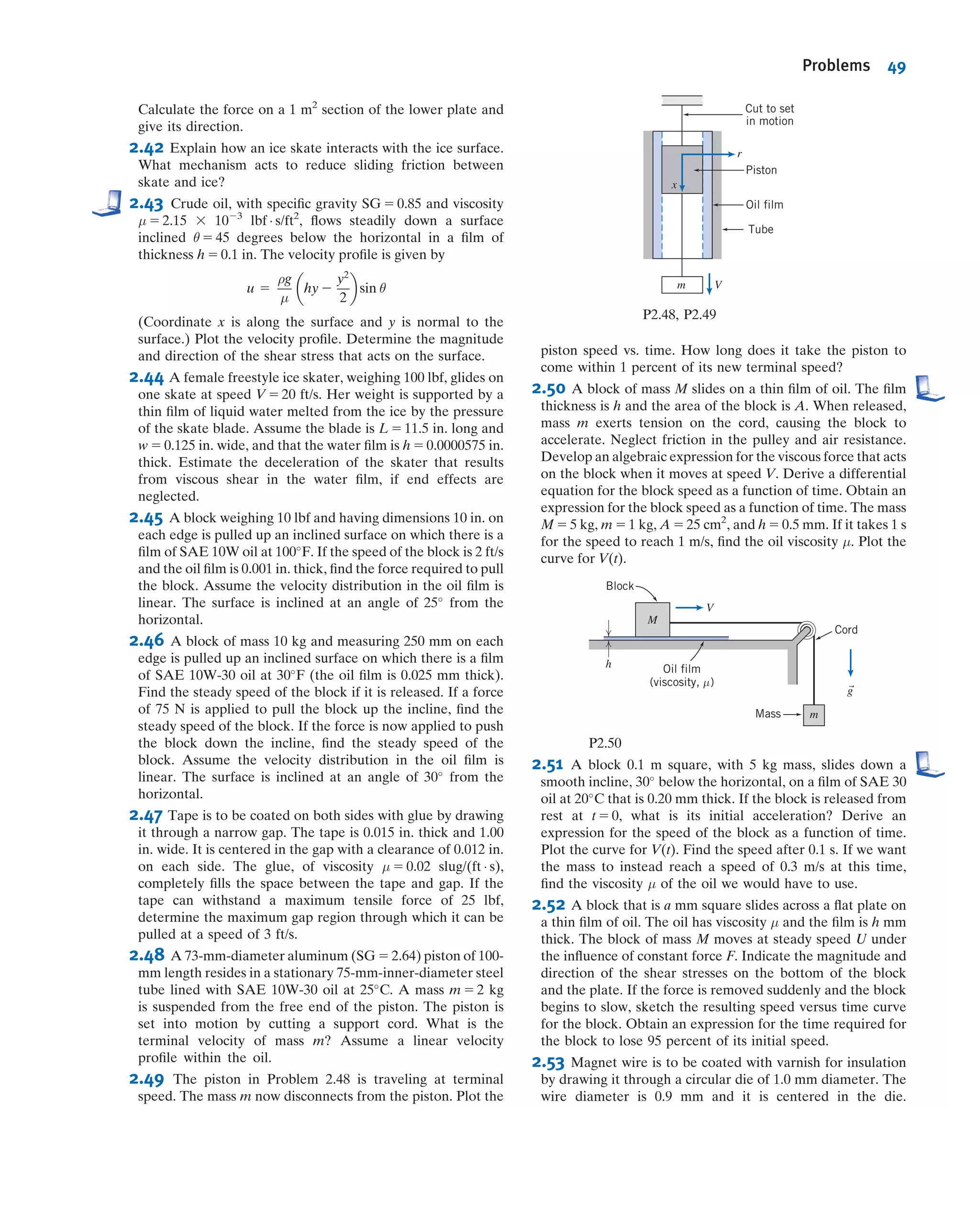
![2.76 A cross section of a rotating bearing is shown. The
spherical member rotates with angular speed ω, a small dis-
tance, a, above the plane surface. The narrow gap is filled
with viscous oil, having μ 5 1250 cp. Obtain an algebraic
expression for the shear stress acting on the spherical
member. Evaluate the maximum shear stress that acts on the
spherical member for the conditions shown. (Is the max-
imum necessarily located at the maximum radius?) Develop
an algebraic expression (in the form of an integral) for the
total viscous shear torque that acts on the spherical member.
Calculate the torque using the dimensions shown.
θ
ω
R = 75 mm
= 70 rpm
a = 0.5 mm
Oil in gap
R0 = 20 mm
P 2.76
Surface Tension
2.77 Small gas bubbles form in soda when a bottle or can is
opened. The average bubble diameter is about 0.1 mm.
Estimate the pressure difference between the inside and
outside of such a bubble.
2.78 You intend to gently place several steel needles on the
free surface of the water in a large tank. The needles come in
two lengths: Some are 5 cm long, and some are 10 cm long.
Needles of each length are available with diameters of 1 mm,
2.5 mm, and 5 mm. Make a prediction as to which needles, if
any, will float.
2.79 According to Folsom [6], the capillary rise Δh (in.) of a
water-air interface in a tube is correlated by the following
empirical expression:
Δh ¼ Ae2 bÁD
where D (in.) is the tube diameter, A 5 0.400, and b 5 4.37.
You do an experiment to measure Δh versus D and obtain:
D (in.) 0.1 0.2 0.3 0.4 0.5 0.6 0.7 0.8 0.9 1 1.1
Δh (in.) 0.232 0.183 0.09 0.059 0.052 0.033 0.017 0.01 0.006 0.004 0.003
What are the values of A and b that best fit this data using
Excel’s Trendline feature? Do they agree with Folsom’s
values? How good is the data?
2.80 Slowly fill a glass with water to the maximum possible
level. Observe the water level closely. Explain how it can be
higher than the rim of the glass.
2.81 Plan an experiment to measure the surface tension of a
liquid similar to water. If necessary, review the NCFMF
video Surface Tension for ideas. Which method would be
most suitable for use in an undergraduate laboratory? What
experimental precision could be expected?
Description and Classification of Fluid Motions
2.82 Water usually is assumed to be incompressible when
evaluating static pressure variations. Actually it is 100 times
more compressible than steel. Assuming the bulk modulus of
water is constant, compute the percentage change in density
for water raised to a gage pressure of 100 atm. Plot the per-
centage change in water density as a function of p/patm up to
a pressure of 50,000 psi, which is the approximate pressure
used for high-speed cutting jets of water to cut concrete and
other composite materials. Would constant density be a rea-
sonable assumption for engineering calculations for cutting
jets?
2.83 The viscous boundary layer velocity profile shown in
Fig. 2.15 can be approximated by a parabolic equation,
uðyÞ 5 a 1 b
y
δ
1 c
y
δ
2
The boundary condition is u 5 U (the free stream velocity) at
the boundary edge δ (where the viscous friction becomes
zero). Find the values of a, b, and c.
2.84 The viscous boundary layer velocity profile shown in
Fig. 2.15 can be approximated by a cubic equation,
uðyÞ 5 a 1 b
y
δ
1 c
y
δ
3
The boundary condition is u 5 U (the free stream velocity)
at the boundary edge δ (where the viscous friction becomes
zero). Find the values of a, b, and c.
2.85 At what minimum speed (in mph) would an automobile
have to travel for compressibility effects to be important?
Assume the local air temperature is 60
F.
2.86 In a food industry process, carbon tetrachloride at 20
C
flows through a tapered nozzle from an inlet diameter Din
5 50 mm to an outlet diameter of Dout. The area varies lin-
early with distance along the nozzle, and the exit area is one-
fifth of the inlet area; the nozzle length is 250 mm. The
flow rate is Q 5 2 L/min. It is important for the process
that the flow exits the nozzle as a turbulent flow. Does it? If
so, at what point along the nozzle does the flow become
turbulent?
2.87 What is the Reynolds number of water at 20
C flowing
at 0.25 m/s through a 5-mm-diameter tube? If the pipe is now
heated, at what mean water temperature will the flow tran-
sition to turbulence? Assume the velocity of the flow remains
constant.
2.88 A supersonic aircraft travels at 2700 km/hr at an alti-
tude of 27 km. What is the Mach number of the aircraft? At
what approximate distance measured from the leading edge
of the aircraft’s wing does the boundary layer change from
laminar to turbulent?
2.89 SAE 30 oil at 100
C flows through a 12-mm-diameter
stainless-steel tube. What is the specific gravity and specific
Problems 53](https://image.slidesharecdn.com/foxphilipj-160402150646/75/Fox-Philip-J-Pritchard-8-ed-Mc-Donald-s-Introduction-to-Fluid-Mechanics-wiley-2011-89-2048.jpg)


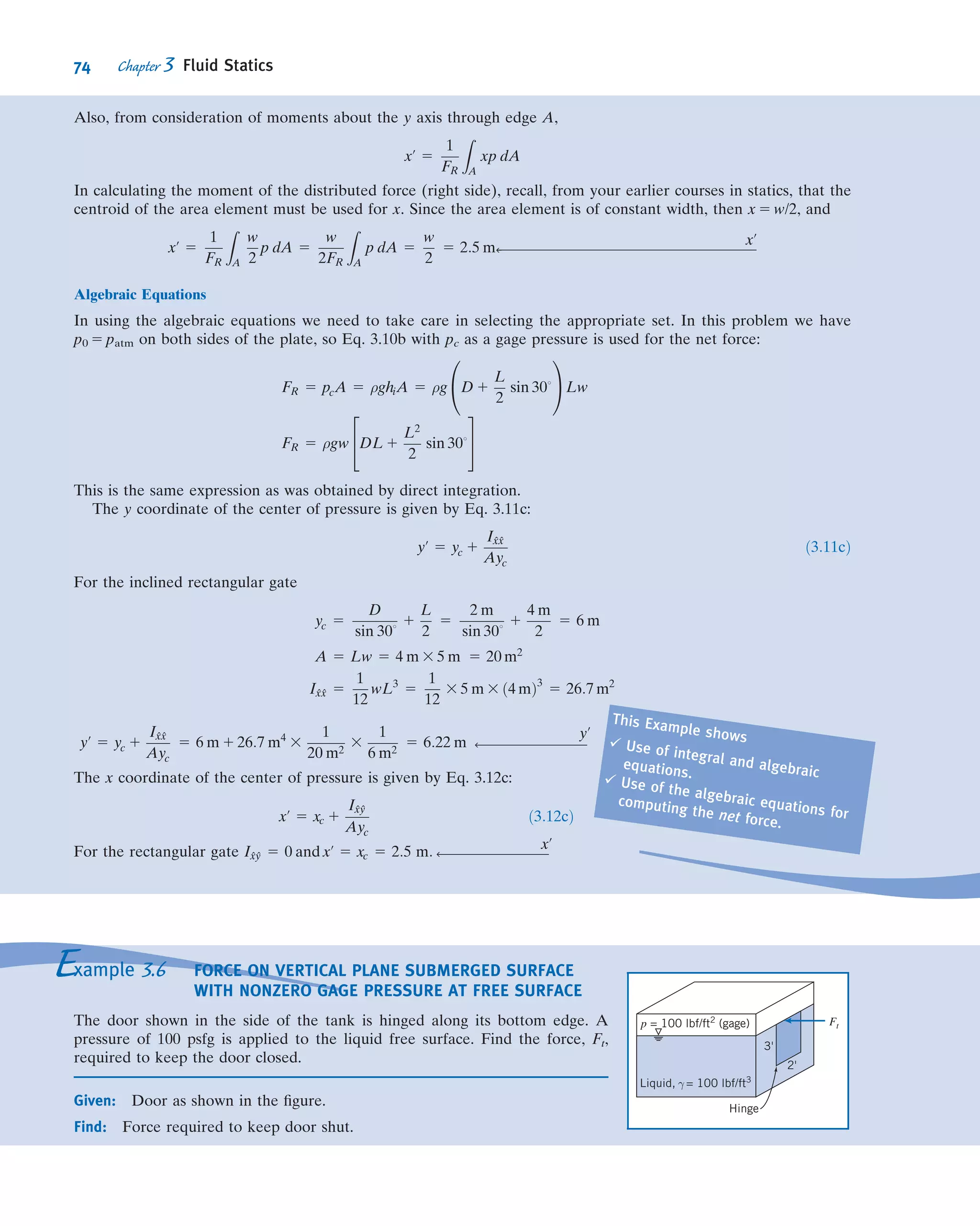


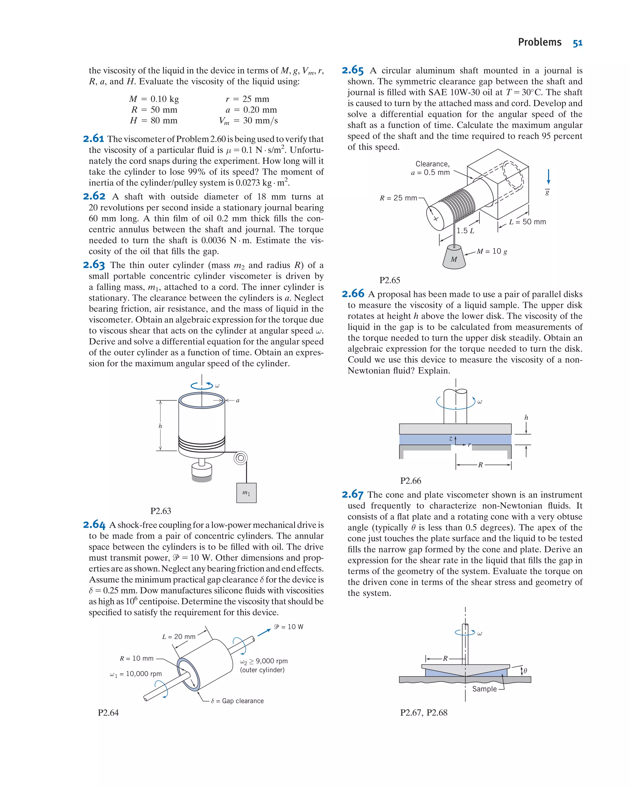
![Governing equations: FH 5 pcA yu 5 yc 1 Ixˆxˆ
Ayc
FV 5 ρgV--- xu 5 water center of gravity
For FH, the centroid, area, and second moment of the equivalent vertical flat plate are, respectively, yc 5 hc 5 D/2,
A 5 Dw, and Ixˆxˆ 5 wD3
/12.
FH 5 pcA 5 ρghcA
5 ρg
D
2
Dw 5 ρg
D2
2
w 5 999
kg
m3
3 9:81
m
s2
3
ð4 m2
Þ
2
3 5 m 3
NUs2
kgUm
FH 5 392 kN
ð1Þ
and
yu 5 yc 1
Ixˆxˆ
Ayc
5
D
2
1
wD3
=12
wDD=2
5
D
2
1
D
6
yu 5
2
3
D 5
2
3
3 4 m 5 2:67 m ð2Þ
For FV, we need to compute the weight of water “above” the gate. To do this we define a differential column of
volume (D 2 y) w dx and integrate
FV 5 ρgV--- 5 ρg
Z D2=a
0
ðD 2 yÞw dx 5 ρgw
Z D2=a
0
ðD 2
ffiffiffi
a
p
x1=2
Þdx
5 ρgw Dx 2
2
3
ffiffiffi
a
p
x3=2
2
4
3
5
D3=a
0
5 ρgw
D3
a
2
2
3
ffiffiffi
a
p D3
a3=2
2
4
3
5 5
ρgwD3
3a
FV 5 999
kg
m3
3 9:81
m
s2
3 5 m 3
ð4Þ3
m3
3
3
1
4 m
3
N Á s2
kg Á m
5 261 kN ð3Þ
The location xu of this force is given by the location of the center of gravity of the water “above” the gate. We
recall from statics that this can be obtained by using the notion that the moment of FV and the moment of the sum of
the differential weights about the y axis must be equal, so
xuFV 5 ρg
Z D2=a
0
xðD 2 yÞw dx 5 ρgw
Z D2=a
0
ðD 2
ffiffiffi
a
p
x3=2
Þdx
xuFV 5 ρgw
D
2
x2
2
2
5
ffiffiffi
a
p
x5=2
2
4
3
5
D2=a
0
5 ρgw
D5
2a2
2
2
5
ffiffiffi
a
p D5
a5=2
2
4
3
5 5
ρgwD5
10a2
xu 5
ρgwD5
10a2FV
5
3D2
10a
5
3
10
3
ð4Þ2
m2
4 m
5 1:2 m ð4Þ
Now that we have determined the fluid forces, we can finally take
moments about O (taking care to use the appropriate signs), using
the results of Eqs. 1 through 4
P
MO 5 2lFa 1 xuFV 1 ðD 2 yuÞFH 5 0
Fa 5
1
l
[xuFV 1 ðD 2 yuÞFH]
5
1
5 m
[1:2 m 3 261 kN 1 ð4 2 2:67Þ m 3 392 kN]
Fa 5 167 kN ß
Fa
This Example shows:ü Use of vertical flat plate equations
for the horizontal force, and fluid
weight equations for the vertical
force, on a curved surface.
ü The use of “thought experiments” to
convert a problem with fluid below a
curved surface into an equivalent
problem with fluid above.
3.5 Hydrostatic Force on Submerged Surfaces 79](https://image.slidesharecdn.com/foxphilipj-160402150646/75/Fox-Philip-J-Pritchard-8-ed-Mc-Donald-s-Introduction-to-Fluid-Mechanics-wiley-2011-115-2048.jpg)
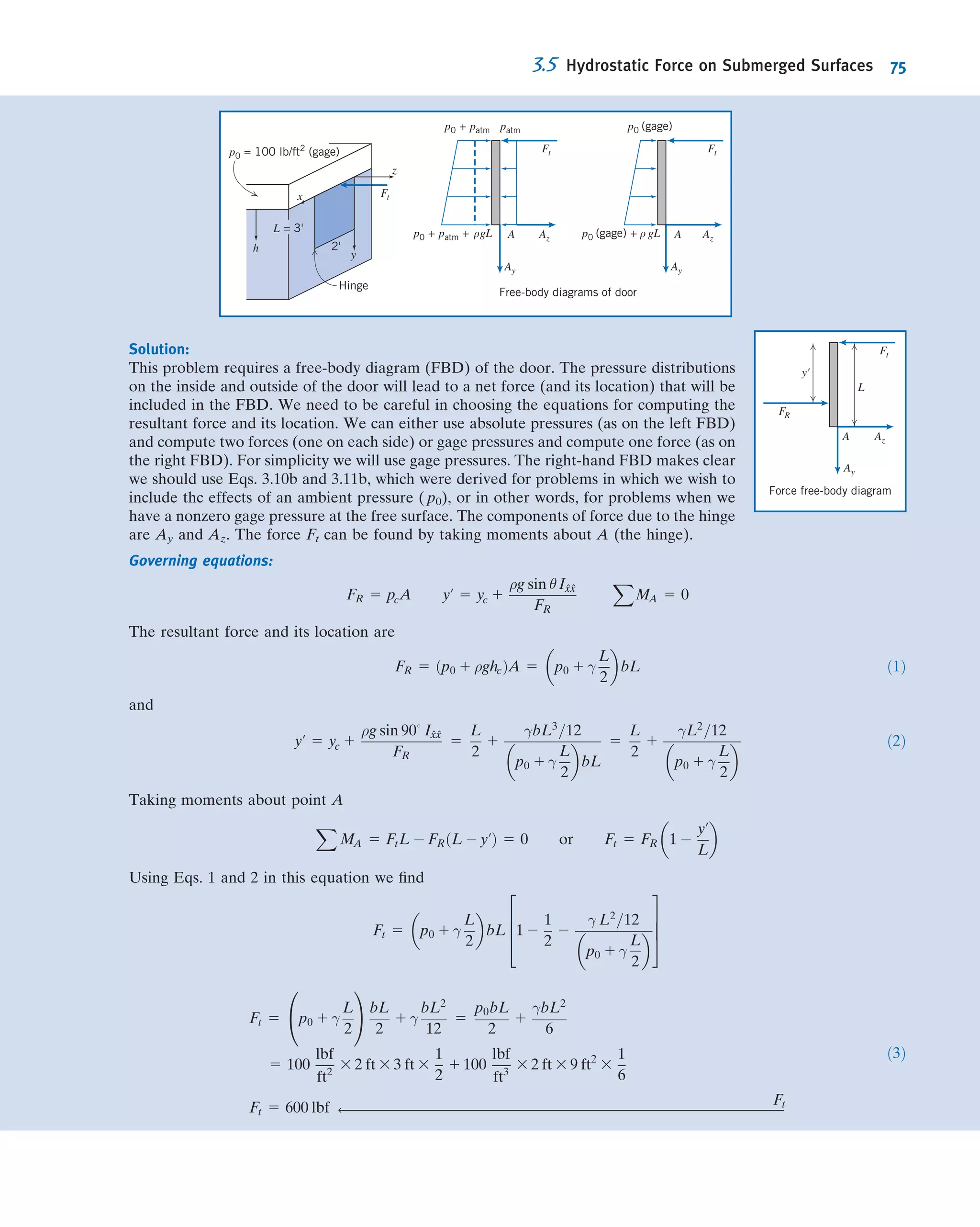
![*3.6 Buoyancy and Stability
If an object is immersed in a liquid, or floating on its surface, the net vertical force
acting on it due to liquid pressure is termed buoyancy. Consider an object totally
immersed in static liquid, as shown in Fig. 3.9.
The vertical force on the body due to hydrostatic pressure may be found most
easily by considering cylindrical volume elements similar to the one shown in Fig. 3.9.
We recall that we can use Eq. 3.7 for computing the pressure p at depth h in a liquid,
p 5 p0 1 ρgh
The net vertical pressure force on the element is then
dFz 5 ð p0 1 ρgh2Þ dA 2 ð p0 1 ρgh1Þ dA 5 ρgðh2 2 h1Þ dA
But ðh2 2 h1ÞdA 5 dV---, the volume of the element. Thus
Fz 5
Z
dFz 5
Z
V---
ρgdV--- 5 ρgV---
where V--- is the volume of the object. Hence we conclude that for a submerged body
the buoyancy force of the fluid is equal to the weight of displaced fluid,
Fbuoyancy 5 ρgV--- ð3:16Þ
This relation reportedly was used by Archimedes in 220 B.C. to determine the gold
content in the crown of King Hiero II. Consequently, it is often called “Archimedes’
Principle.” In more current technical applications, Eq. 3.16 is used to design dis-
placement vessels, flotation gear, and submersibles [1].
The submerged object need not be solid. Hydrogen bubbles, used to visualize
streaklines and timelines in water (see Section 2.2), are positively buoyant; they rise
slowly as they are swept along by the flow. Conversely, water droplets in oil are
negatively buoyant and tend to sink.
Airships andballoons are termed“lighter-than-air” craft. Thedensity of an ideal gas is
proportional to molecular weight, so hydrogen and helium are less dense than air at the
same temperature and pressure. Hydrogen (Mm 5 2) is less dense than helium (Mm 5 4),
but extremely flammable, whereas helium is inert. Hydrogen has not been used com-
mercially since the disastrous explosion of the German passenger airship Hindenburg in
1937. The use of buoyancy force to generate lift is illustrated in Example 3.8.
Equation 3.16 predicts the net vertical pressure force on a body that is totally
submerged in a single liquid. In cases of partial immersion, a floating body displaces its
own weight of the liquid in which it floats.
The line of action of the buoyancy force, which may be found using the methods of
Section 3.5, acts through the centroid of the displaced volume. Since floating bodies
z
h
h1
h2
p0
Liquid,
density = ρd
dA
V
Fig. 3.9 Immersed body in static liquid.
1
This section may be omitted without loss of continuity in the text material.
80 Chapter 3 Fluid Statics](https://image.slidesharecdn.com/foxphilipj-160402150646/75/Fox-Philip-J-Pritchard-8-ed-Mc-Donald-s-Introduction-to-Fluid-Mechanics-wiley-2011-116-2048.jpg)
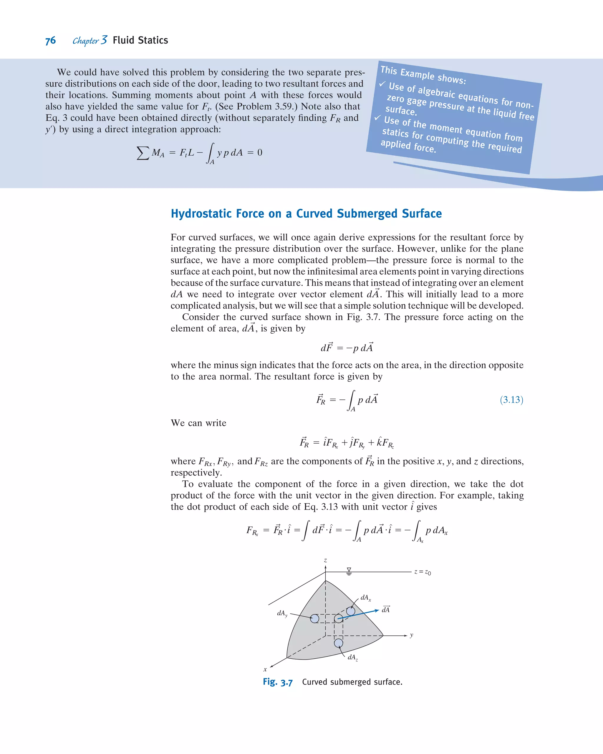
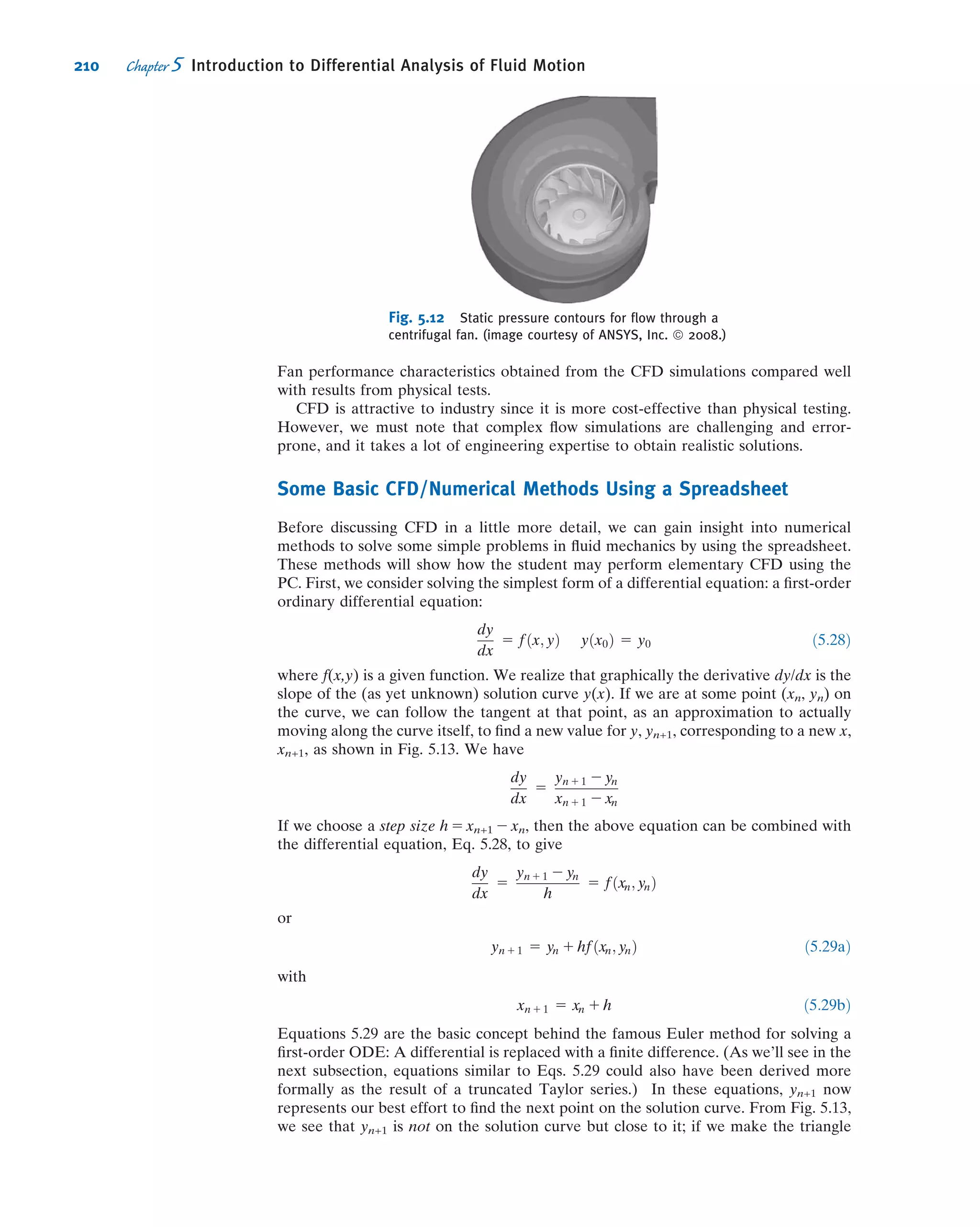
![Modern ships can have stability problems as well: overloaded ferry boats have cap-
sized when passengers all gathered on one side of the upper deck, shifting the CG
laterally. In stacking containers high on the deck of a container ship, care is needed to
avoid raising the center of gravity to a level that may result in the unstable condition
depicted in Fig. 3.10b.
For a vessel with a relatively flat bottom, as shown in Fig. 3.10a, the restoring
moment increases as roll angle becomes larger. At some angle, typically that at which
the edge of the deck goes below water level, the restoring moment peaks and starts to
decrease. The moment may become zero at some large roll angle, known as the angle
of vanishing stability. The vessel may capsize if the roll exceeds this angle; then, if still
intact, the vessel may find a new equilibrium state upside down.
The actual shape of the restoring moment curve depends on hull shape. A broad
beam gives a large lateral shift in the line of action of the buoyancy force and thus a high
restoring moment. High freeboard above the water line increases the angle at which the
moment curve peaks, but may make the moment drop rapidly above this angle.
Sailing vessels are subjected to large lateral forces as wind engages the sails (a boat
under sail in a brisk wind typically operates at a considerable roll angle). The lateral
wind force must be counteracted by a heavily weighted keel extended below the hull
bottom. In small sailboats, crew members may lean far over the side to add additional
restoring moment to prevent capsizing [2].
Within broad limits, the buoyancy of a surface vessel is adjusted automatically as
the vessel rides higher or lower in the water. However, craft that operate fully sub-
merged must actively adjust buoyancy and gravity forces to remain neutrally buoyant.
For submarines this is accomplished using tanks which are flooded to reduce excess
buoyancy or blown out with compressed air to increase buoyancy [1]. Airships may
vent gas to descend or drop ballast to rise. Buoyancy of a hot-air balloon is controlled
by varying the air temperature within the balloon envelope.
For deep ocean dives use of compressed air becomes impractical because of the high
pressures (the Pacific Ocean is over 10 km deep; seawater pressure at this depth is
greater than 1000 atmospheres!). A liquid such as gasoline, which is buoyant in seawater,
may be used to provide buoyancy. However, because gasoline is more compressible than
water, its buoyancy decreases as the dive gets deeper. Therefore it is necessary to carry
and drop ballast to achieve positive buoyancy for the return trip to the surface.
The most structurally efficient hull shape for airships and submarines has a circular
cross-section. The buoyancy force passes through the center of the circle. Therefore,
for roll stability the CG must be located below the hull centerline. Thus the crew
compartment of an airship is placed beneath the hull to lower the CG.
3.7 Fluids in Rigid-Body Motion (on the Web)
buoyancy
buoyancygravity
gravity
(a) Stable (b) Unstable
CG
CG
Fig. 3.10 Stability of floating bodies.
82 Chapter 3 Fluid Statics](https://image.slidesharecdn.com/foxphilipj-160402150646/75/Fox-Philip-J-Pritchard-8-ed-Mc-Donald-s-Introduction-to-Fluid-Mechanics-wiley-2011-118-2048.jpg)


![For uniform properties, assumption (2), we can write
ϩ gz1)(Ϫ 1V1A1) ϩ (h2 ϩQ ϭ Ws ϩ (h1 ϩ
Ϸ0(6)
V1
2
2
ϩ gz2)( 2V2A2)
V2
2
2
For steady flow, from conservation of mass,
Z
CS
ρ ~V Á d ~A 5 0
Therefore, 2(ρ1V1A1) 1 (ρ2V2A2) 5 0, or ρ1V1A1 5 ρ2V2A2 5 _m. Hence we can write
Q ϭ Ws ϩ m [(h2 Ϫ h1) ϩ ϩ g(z2 Ϫ z1)]
ϭ0(5)
V2
2
2
Assume that air behaves as an ideal gas with constant cp. Then h2 2 h1 5 cp(T2 2 T1), and
_Q 5 _Ws 1 _m cpðT2 2 T1Þ 1
V2
2
2
From continuity V2 5 _m=ρ2A2. Since p2 5 ρ2RT2,
V2 5
_m
A2
RT2
p2
5 20
lbm
s
3
1
1 ft2
3 53:3
ft Á lbf
lbmÁ3R
3 5603
R 3
in:2
50 lbf
3
ft2
144 in:2
V2 5 82:9 ft=s
Note that power input is to the CV, so _Ws 5 2600 hp, and
_Q 5 _Ws 1 _mcp ðT2 2 T1Þ 1 _m
V2
2
2
_Q 5 2600 hp 3 550
ft Á lbf
hp Á s
3
Btu
778 ft Á lbf
1 20
lbm
s
3 0:24
Btu
lbm Á R
3 30
R
1 20
lbm
s
3
ð82:9Þ2
2
ft2
s2
3
slug
32:2 lbm
3
Btu
778 ft Á lbf
3
lbf Á s2
slug Á ft
_Q 5 2277 Btu=sß
fheat rejectiong _Q
This problem illustrates use of the first
law of thermodynamics for a control
volume. It is also an example of the
care that must be taken with unit con-
versions for mass, energy, and power.
Example 4.17 TANK FILLING: FIRST LAW ANALYSIS
A tank of 0.1 m3
volume is connected to a high-pressure air line; both line and tank are initially at a uniform
temperature of 20
C. The initial tank gage pressure is 100 kPa. The absolute line pressure is 2.0 MPa; the line is large
enough so that its temperature and pressure may be assumed constant. The tank temperature is monitored by a fast-
response thermocouple. At the instant after the valve is opened, the tank temperature rises at the rate of 0.05
C/s.
Determine the instantaneous flow rate of air into the tank if heat transfer is neglected.
144 Chapter 4 Basic Equations in Integral Form for a Control Volume](https://image.slidesharecdn.com/foxphilipj-160402150646/75/Fox-Philip-J-Pritchard-8-ed-Mc-Donald-s-Introduction-to-Fluid-Mechanics-wiley-2011-188-2048.jpg)


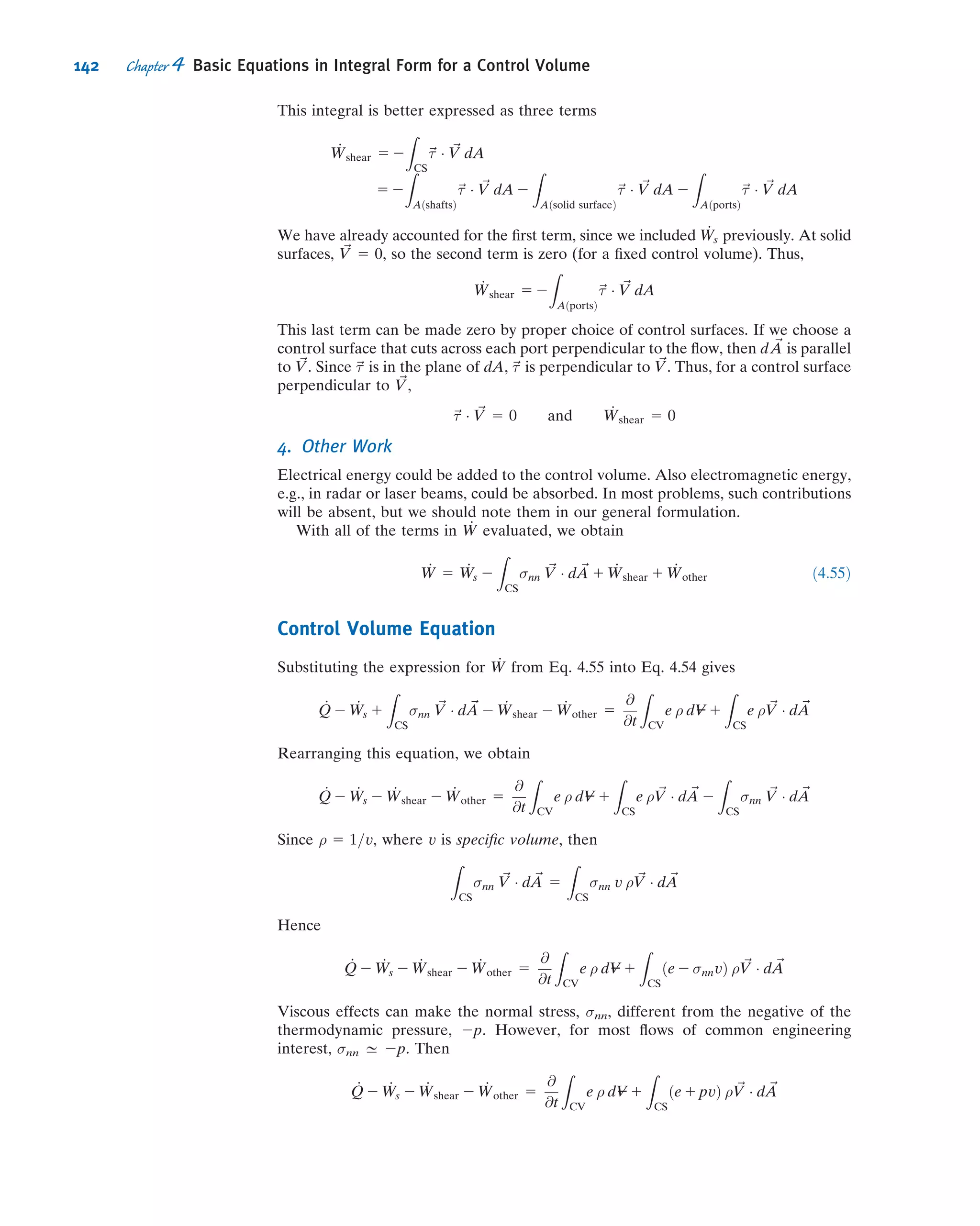
![4.52 Water flows steadily past a porous flat plate. Constant
suction is applied along the porous section. The velocity
profile at section cd is
u
UN
5 3
y
δ
h i
2 2
y
δ
h i3=2
Evaluate the mass flow rate across section bc.
L = 2 m
V = –0.2j mm/s
^ d
a
c
u δ = 1.5 mm
Width,
w = 1.5 m
y
x
U = 3 m/s
b
P4.52, P4.53
4.53 Consider incompressible steady flow of standard air in a
boundary layer on the length of porous surface shown.
Assume the boundary layer at the downstream end of the
surface has an approximately parabolic velocity profile,
u/UN 5 2(y/δ) 2 (y/δ)2
. Uniform suction is applied along
the porous surface, as shown. Calculate the volume flow
rate across surface cd, through the porous suction surface,
and across surface bc.
4.54 A tank of fixed volume contains brine with initial
density, ρi, greater than water. Pure water enters the tank
steadily and mixes thoroughly with the brine in the tank. The
liquid level in the tank remains constant. Derive expressions
for (a) the rate of change of density of the liquid mixture
in the tank and (b) the time required for the density to reach
the value ρf, where ρi . ρf . ρH2O.
min
•
ρ
mout
•
ρ
H2
O
V = constant
P4.54
4.55 A conical funnel of half-angle θ 5 30
drains through a
small hole of diameter d 5 0.25 in. at the vertex. The speed
of the liquid leaving the funnel is approximately V ¼
ffiffiffiffiffiffiffiffi
2gy
p
,
where y is the height of the liquid free surface above the
hole. The funnel initially is filled to height y0 5 12 in. Obtain
an expression for the time, t, for the funnel to completely
drain, and evaluate. Find the time to drain from 12 in. to 6 in.
(a change in depth of 6 in.), and from 6 in. to completely
empty (also a change in depth of 6 in.). Can you explain the
discrepancy in these times? Plot the drain time t as a function
diameter d for d ranging from 0.25 in. to 0.5 in.
4.56 For the funnel of Problem 4.55, find the diameter d
required if the funnel is to drain in t 5 1 min. from an initial
depth y0 5 12 in. Plot the diameter d required to drain the
funnel in 1 min as a function of initial depth y0, for y0 ranging
from 1 in. to 24 in.
4.57 Over time, air seeps through pores in the rubber of high-
pressure bicycle tires. The saying is that a tire loses pressure at
the rate of “a pound [1 psi] a day.” The true rate of pressure
loss is not constant; instead, the instantaneous leakage mass
flow rate is proportional to the air density in the tire and to the
gage pressure in the tire, _m~ρp. Because the leakage rate is
slow, air in the tire is nearly isothermal. Consider a tire that
initially is inflated to 0.6 MPa (gage). Assume the initial rate
of pressure loss is 1 psi per day. Estimate how long it will take
for the pressure to drop to 500 kPa. How accurate is “a pound
a day” over the entire 30 day period? Plot the pressure as a
function of time over the 30 day period. Show the rule-of-
thumb results for comparison.
Momentum Equation for Inertial Control Volume
4.58 Evaluate the net rate of flux of momentum out through
the control surface of Problem 4.24.
4.59 For the conditions of Problem 4.34, evaluate the ratio of
the x-direction momentum flux at the channel outlet to that
at the inlet.
4.60 For the conditions of Problem 4.35, evaluate the ratio of
the x-direction momentum flux at the pipe outlet to that at
the inlet.
4.61 Evaluate the net momentum flux through the bend of
Problem 4.38, if the depth normal to the diagram is w 5 1 m.
4.62 Evaluate the net momentum flux through the channel
of Problem 4.39. Would you expect the outlet pressure to be
higher, lower, or the same as the inlet pressure? Why?
4.63 Water jets are being used more and more for metal
cutting operations. If a pump generates a flow of 1 gpm
through an orifice of 0.01 in. diameter, what is the average jet
speed? What force (lbf) will the jet produce at impact,
assuming as an approximation that the water sprays sideways
after impact?
4.64 Considering that in the fully developed region of a pipe,
the integral of the axial momentum is the same at all cross
sections, explain the reason for the pressure drop along
the pipe.
4.65 Find the force required to hold the plug in place at the
exit of the water pipe. The flow rate is 1.5 m3
/s, and the
upstream pressure is 3.5 MPa.
F
0.2 m0.25 m
P4.65
4.66 A jet of water issuing from a stationary nozzle at 10 m/s
(Aj 5 0.1 m2
) strikes a turning vane mounted on a cart as
shown. The vane turns the jet through angle θ 5 40
.
Determine the value of M required to hold the cart sta-
tionary. If the vane angle θ is adjustable, plot the mass, M,
needed to hold the cart stationary versus θ for 0 # θ # 180
.
154 Chapter 4 Basic Equations in Integral Form for a Control Volume](https://image.slidesharecdn.com/foxphilipj-160402150646/75/Fox-Philip-J-Pritchard-8-ed-Mc-Donald-s-Introduction-to-Fluid-Mechanics-wiley-2011-198-2048.jpg)


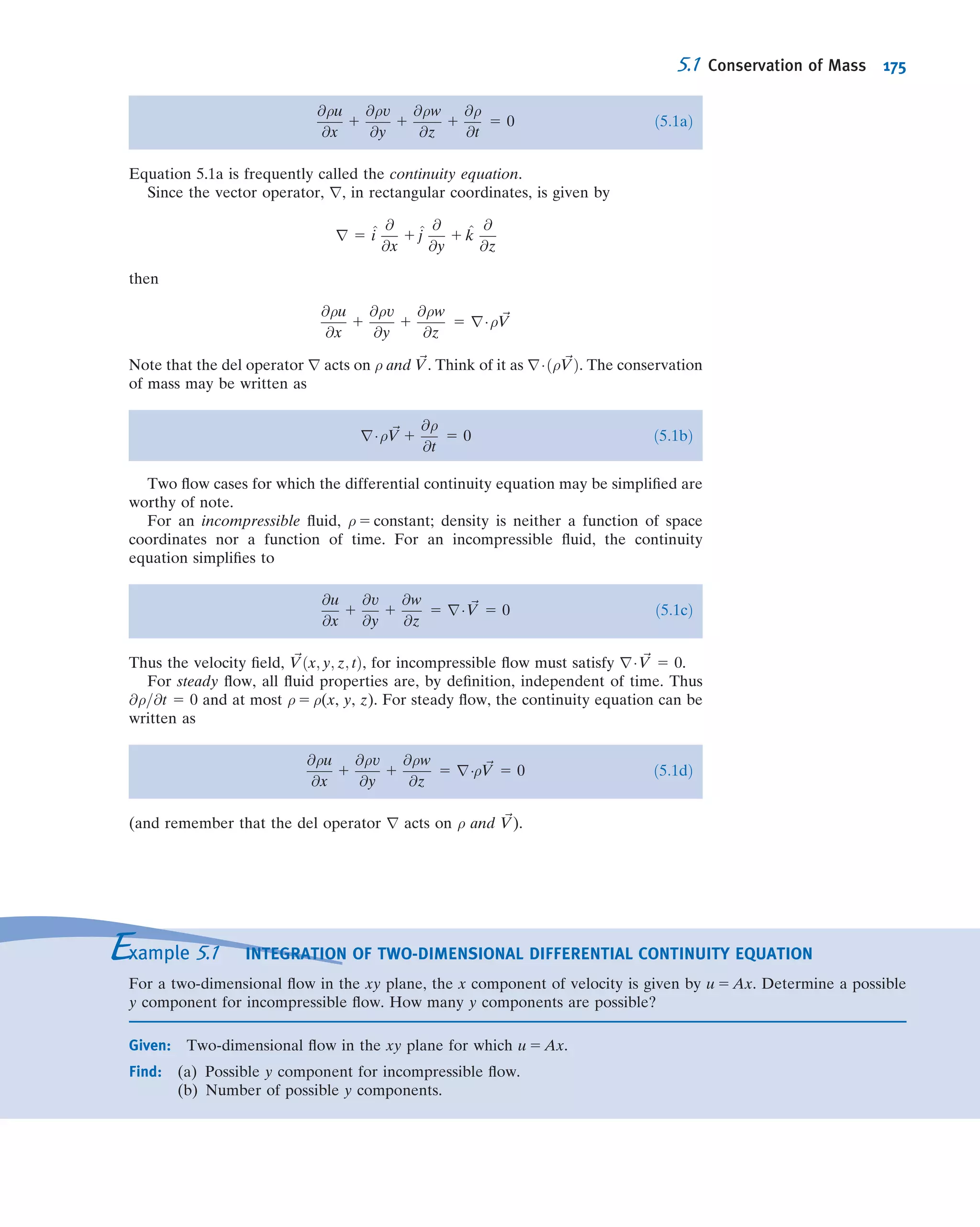
![Table 5.1 shows the details of this evaluation. Note: We assume that the velocity
components u, v, and w are positive in the x, y, and z directions, respectively; the area
normal is by convention positive out of the cube; and higher-order terms [e.g., (dx)2
]
are neglected in the limit as dx, dy, and dz - 0.
The result of all this work is
@ρu
@x
1
@ρv
@x
1
@ρw
@x
dx dy dz
This expression is the surface integral evaluation for our differential cube. To com-
plete Eq. 4.12, we need to evaluate the volume integral (recall that @=@t
R
CV ρdV--- is the
rate of change of mass in the control volume):
@
@t
Z
CV
ρdV----
@
@t
½ρdx dy dzŠ 5
@ρ
@t
dx dy dz
Hence, we obtain (after canceling dx dy dz) from Eq. 4.12 a differential form of the
mass conservation law
Table 5.1
Mass Flux Through the Control Surface of a Rectangular Differential Control Volume
Surface Evaluation of
Z
ρ~V Ád~A
Left
ð2xÞ
5 2 ρ 2
@ρ
@x
dx
2
u 2
@u
@x
dx
2
dy dz 5 2ρu dy dz 1
1
2
u
@ρ
@x
1 ρ
@u
@x
dx dy dz
Right
ð1xÞ
5 ρ 1
@ρ
@x
dx
2
u 1
@u
@x
dx
2
dy dz 5 ρu dy dz 1
1
2
u
@ρ
@x
1 ρ
@u
@x
dx dy dz
Bottom
ð2yÞ
5 2 ρ 2
@ρ
@y
dy
2
v 2
@v
@y
dy
2
dx dz 5 2ρv dx dz 1
1
2
v
@ρ
@y
1 ρ
@v
@y
dx dy dz
Top
ð1yÞ
5 ρ 1
@ρ
@y
dy
2
v 1
@v
@y
dy
2
dx dz 5 ρv dx dz 1
1
2
v
@ρ
@y
1 ρ
@v
@y
dx dy dz
Back
ð2zÞ
5 2 ρ 2
@ρ
@z
dz
2
w 2
@w
@z
dz
2
dx dy 5 2ρw dx dy 1
1
2
w
@ρ
@z
1 ρ
@w
@z
dx dy dz
Front
ð1zÞ
5 ρ 1
@ρ
@z
dz
2
w 1
@w
@z
dz
2
dx dy 5 ρw dx dy 1
1
2
w
@ρ
@z
1 ρ
@w
@z
dx dy dz
Adding the results for all six faces,
Z
CS
ρ ~VÁd ~A 5 u
@ρ
@x
1 ρ
@u
@x
1 v
@ρ
@y
1 ρ
@v
@y
1 w
@ρ
@z
1 ρ
@w
@z
dx dy dz
or
Z
CS
ρ ~V Ád ~A 5
@ρu
@x
1
@ρv
@y
1
@ρw
@z
dx dy dz
174 Chapter 5 Introduction to Differential Analysis of Fluid Motion](https://image.slidesharecdn.com/foxphilipj-160402150646/75/Fox-Philip-J-Pritchard-8-ed-Mc-Donald-s-Introduction-to-Fluid-Mechanics-wiley-2011-218-2048.jpg)


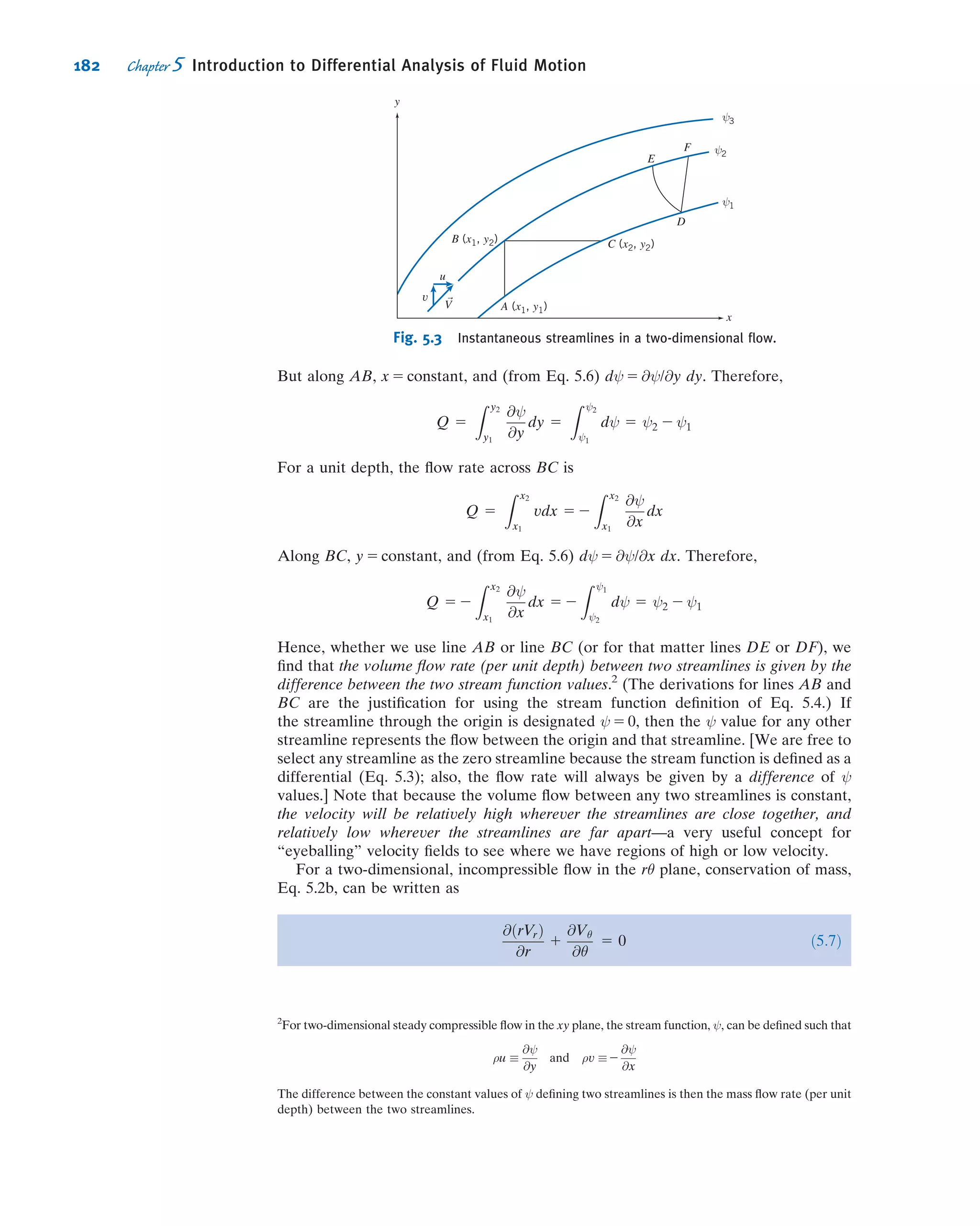
![But along AB, x 5 constant, and (from Eq. 5.6) dψ 5 @ψ/@y dy. Therefore,
Q 5
Z y2
y1
@ψ
@y
dy 5
Z ψ2
ψ1
dψ 5 ψ2 2 ψ1
For a unit depth, the flow rate across BC is
Q 5
Z x2
x1
vdx 5 2
Z x2
x1
@ψ
@x
dx
Along BC, y 5 constant, and (from Eq. 5.6) dψ 5 @ψ/@x dx. Therefore,
Q 5 2
Z x2
x1
@ψ
@x
dx 5 2
Z ψ1
ψ2
dψ 5 ψ2 2 ψ1
Hence, whether we use line AB or line BC (or for that matter lines DE or DF), we
find that the volume flow rate (per unit depth) between two streamlines is given by the
difference between the two stream function values.2
(The derivations for lines AB and
BC are the justification for using the stream function definition of Eq. 5.4.) If
the streamline through the origin is designated ψ 5 0, then the ψ value for any other
streamline represents the flow between the origin and that streamline. [We are free to
select any streamline as the zero streamline because the stream function is defined as a
differential (Eq. 5.3); also, the flow rate will always be given by a difference of ψ
values.] Note that because the volume flow between any two streamlines is constant,
the velocity will be relatively high wherever the streamlines are close together, and
relatively low wherever the streamlines are far apart—a very useful concept for
“eyeballing” velocity fields to see where we have regions of high or low velocity.
For a two-dimensional, incompressible flow in the rθ plane, conservation of mass,
Eq. 5.2b, can be written as
@ðrVrÞ
@r
1
@Vθ
@θ
5 0 ð5:7Þ
y
x
A (x1, y1)
C (x2, y2)B (x1, y2)
D
E
F
V
u
ψ3
ψ2
ψ1
v
Fig. 5.3 Instantaneous streamlines in a two-dimensional flow.
2
For two-dimensional steady compressible flow in the xy plane, the stream function, ψ, can be defined such that
ρu
@ψ
@y
and ρv 2
@ψ
@x
The difference between the constant values of ψ defining two streamlines is then the mass flow rate (per unit
depth) between the two streamlines.
182 Chapter 5 Introduction to Differential Analysis of Fluid Motion](https://image.slidesharecdn.com/foxphilipj-160402150646/75/Fox-Philip-J-Pritchard-8-ed-Mc-Donald-s-Introduction-to-Fluid-Mechanics-wiley-2011-230-2048.jpg)

![Now we can determine from Δα and Δβ a measure of the particle’s angular
deformation, as shown in Fig. 5.7d. To obtain the deformation of side oa in Fig. 5.7d,
we use Fig. 5.7b and 5.7c: If we subtract the particle rotation 1
2(Δα 2 Δβ), in Fig. 5.7c,
from the actual rotation of oa, Δα, in Fig. 5.7b, what remains must be pure defor-
mation [Δα 2 1
2(Δα 2 Δβ) 5 1
2(Δα 1 Δβ), in Fig. 5.7d]. Using the assigned values, the
deformation of side oa is 6
2 1
2(6
2 4
) 5 5
. By a similar process, for side ob we end
with Δβ 2 1
2(Δα 2 Δβ) 521
2(Δα 1 Δβ), or a clockwise deformation 1
2(Δα 1 Δβ), as
shown in Fig. 5.7d. The total deformation of the particle is the sum of the deforma-
tions of the sides, or (Δα 1 Δβ) (with our example values, 10
). We verify that this
leaves us with the correct value for the particle’s deformation: Recall that in Section
2.4 we saw that deformation is measured by the change in a 90
angle. In Fig. 5.7a we
see this is angle aob, and in Fig. 5.7d we see the total change of this angle is indeed
1
2(Δα 1 Δβ) 1 1
2(Δα 1 Δβ) 5 (Δα 1 Δβ).
We need to convert these angular measures to quantities obtainable from the flow
field. To do this, we recognize that (for small angles) Δα 5 Δη=Δx, and
Δβ 5 Δξ=Δy. But Δξ arises because, if in interval Δt point o moves horizontally
distance uΔt, then point b will have moved distance ðu 1 ½@u=@yŠΔyÞΔt (using a
Taylor series expansion). Likewise, Δη arises because, if in interval Δt point o moves
vertically distance vΔt, then point a will have moved distance ðv 1 ½@v=@xŠΔxÞΔt.
Hence,
Δξ 5 u 1
@u
@y
Δy
Δt 2 uΔt 5
@u
@y
ΔyΔt
and
Δη 5 v 1
@v
@x
Δx
Δt 2 vΔt 5
@v
@x
ΔxΔt
We can now compute the angular velocity of the particle about the z axis, ωz, by
combining all these results:
ωz 5 lim
Δt-0
1
2
ðΔα 2 ΔβÞ
Δt
5 lim
Δt-0
1
2
Δη
Δx
2
Δξ
Δy
Δt
5 lim
Δt-0
1
2
@v
@x
Δx
Δx
Δt 2
@u
@y
Δy
Δy
Δt
Δt
ωz 5
1
2
@v
@x
2
@u
@y
By considering the rotation of pairs of perpendicular line segments in the yz and xz
planes, one can show similarly that
ωx 5
1
2
@w
@y
2
@v
@z
and ωy 5
1
2
@u
@z
2
@w
@x
Then ~ω 5 ^iωx 1 ^jωy 1 ^kωz becomes
~ω 5
1
2
^i
@w
@y
2
@v
@z
1 ^j
@u
@z
2
@w
@x
1 ^k
@v
@x
2
@u
@y
ð5:13Þ
We recognize the term in the square brackets as
curl ~V 5 r 3 ~V
5.3 Motion of a Fluid Particle (Kinematics) 191](https://image.slidesharecdn.com/foxphilipj-160402150646/75/Fox-Philip-J-Pritchard-8-ed-Mc-Donald-s-Introduction-to-Fluid-Mechanics-wiley-2011-239-2048.jpg)


![On simplifying, we obtain
dFSx
5
@σxx
@x
1
@τyx
@y
1
@τzx
@z
dxdydz
When the force of gravity is the only body force acting, then the body force per unit
mass is ~g. The net force in the x direction, dFx, is given by
dFx 5 dFBx
1 dFSx
5 ρgx 1
@σxx
@x
1
@τyx
@y
1
@τzx
@z
dxdydz ð5:23aÞ
We can derive similar expressions for the force components in the y and z directions:
dFy 5 dFBy
1 dFSy
5 ρgy 1
@τxy
@x
1
@σyy
@y
1
@τzy
@z
dxdydz ð5:23bÞ
dFz 5 dFBz
1 dFSz
5 ρgz 1
@τxz
@x
1
@τyz
@y
1
@σzz
@z
dxdydz ð5:23cÞ
Differential Momentum Equation
We have now formulated expressions for the components, dFx, dFy, and dFz, of the
force, d~F, acting on the element of mass dm. If we substitute these expressions
(Eqs. 5.23) for the force components into the x, y, and z components of Eq. 5.22, we
obtain the differential equations of motion,
ρgx 1
@σxx
@x
1
@τyx
@y
1
@τzx
@z
5 ρ
@u
@t
1 u
@u
@x
1 v
@u
@y
1 w
@u
@z
ð5:24aÞ
ρgy 1
@τxy
@x
1
@σyy
@y
1
@τzy
@z
5 ρ
@v
@t
1 u
@v
@x
1 v
@v
@y
1 w
@v
@z
ð5:24bÞ
ρgz 1
@τxz
@x
1
@τyz
@y
1
@σzz
@z
5 ρ
@w
@t
1 u
@w
@x
1 v
@w
@y
1 w
@w
@z
ð5:24cÞ
Equations 5.24 are the differential equations of motion for any fluid satisfying the
continuum assumption. Before the equations can be used to solve for u, v, and w,
suitable expressions for the stresses must be obtained in terms of the velocity and
pressure fields.
Newtonian Fluid: NavierÀStokes Equations
For a Newtonian fluid the viscous stress is directly proportional to the rate of shearing
strain (angular deformation rate). We saw in Chapter 2 that for one-dimensional
laminar Newtonian flow the shear stress is proportional to the rate of angular defor-
mation: τyx 5 du/dy (Eq. 2.15). For a three-dimensional flow the situation is a bit more
complicated (among other things we need to use the more complicated expressions for
rate of angular deformation, Eq. 5.19). The stresses may be expressed in terms of
velocity gradients and fluid properties in rectangular coordinates as follows:6
6
The derivation of these results is beyond the scope of this book. Detailed derivations may be found in Daily
and Harleman [2], Schlichting [3], and White [4].
5.4 Momentum Equation 199](https://image.slidesharecdn.com/foxphilipj-160402150646/75/Fox-Philip-J-Pritchard-8-ed-Mc-Donald-s-Introduction-to-Fluid-Mechanics-wiley-2011-247-2048.jpg)
![τxy 5 τyx 5 μ
@v
@x
1
@u
@y
ð5:25aÞ
τyz 5 τzy 5 μ
@w
@y
1
@v
@z
ð5:25bÞ
τzx 5 τxz 5 μ
@u
@z
1
@w
@x
ð5:25cÞ
σxx 5 2p 2
2
3
μrÁ ~V 1 2μ
@u
@x
ð5:25dÞ
σyy 5 2p 2
2
3
μrÁ ~V 1 2μ
@v
@y
ð5:25eÞ
σzz 5 2p 2
2
3
μrÁ ~V 1 2μ
@w
@z
ð5:25fÞ
where p is the local thermodynamic pressure.7
Thermodynamic pressure is related to
the density and temperature by the thermodynamic relation usually called the
equation of state.
If these expressions for the stresses are introduced into the differential equations of
motion (Eqs. 5.24), we obtain
ρ
Du
Dt
5 ρgx 2
@p
@x
1
@
@x
μ
2
@u
@x
2
2
3
rÁ ~V
1
@
@y
μ
@u
@y
1
@v
@x
1
@
@z
μ
@w
@x
1
@u
@z
ð5:26aÞ
ρ
Dv
Dt
5 ρgy 2
@p
@y
1
@
@x
μ
@u
@y
1
@v
@x
1
@
@y
μ
2
@v
@y
2
2
3
rÁ ~V
1
@
@z
μ
@v
@z
1
@w
@y
ð5:26bÞ
ρ
Dw
Dt
5 ρgz 2
@p
@z
1
@
@x
μ
@w
@x
1
@u
@z
1
@
@y
μ
@w
@z
1
@w
@y
1
@
@z
μ
2
@w
@z
2
2
3
rÁ ~V
ð5:26cÞ
These equations of motion are called the NavierÀStokes equations. The equations are
greatly simplified when applied to incompressible flow with constant viscosity. Under
these conditions the equations reduce to
ρ
@u
@t
1 u
@u
@x
1 v
@u
@y
1 w
@u
@z
5 ρgx 2
@p
@x
1 μ
@2
u
@x2
1
@2
u
@y2
1
@2
u
@z2
ð5:27aÞ
7
Sabersky et al. [5] discuss the relation between the thermodynamic pressure and the average pressure
defined as p 5 2 ðσxx 1 σyy 1 σzzÞ=3.
200 Chapter 5 Introduction to Differential Analysis of Fluid Motion](https://image.slidesharecdn.com/foxphilipj-160402150646/75/Fox-Philip-J-Pritchard-8-ed-Mc-Donald-s-Introduction-to-Fluid-Mechanics-wiley-2011-248-2048.jpg)
![ρ
@v
@t
1 u
@v
@x
1 v
@v
@y
1 w
@v
@z
5 ρgy 2
@p
@y
1 μ
@2
v
@x2
1
@2
v
@y2
1
@2
v
@z2
ð5:27bÞ
ρ
@w
@t
1 u
@w
@x
1 v
@w
@y
1 w
@w
@z
5 ρgz 2
@p
@z
1 μ
@2
w
@x2
1
@2
w
@y2
1
@2
w
@z2
ð5:27cÞ
This form of the NavierÀStokes equations is probably (next to the Bernoulli equa-
tion) the most famous set of equations in fluid mechanics, and has been widely
studied. These equations, with the continuity equation (Eq. 5.1c), form a set of four
coupled nonlinear partial differential equations for u, v, w, and p. In principle, these
four equations describe many common flows; the only restrictions are that the fluid be
Newtonian (with a constant viscosity) and incompressible. For example, lubrication
theory (describing the behavior of machine bearings), pipe flows, and even the motion
of your coffee as you stir it are explained by these equations. Unfortunately, they are
impossible to solve analytically, except for the most basic cases [3], in which we have
simple boundaries and initial or boundary conditions! We will solve the equations for
such a simple problem in Example 5.9.
The NavierÀStokes equations for constant density and viscosity are given in
cylindrical coordinates in Appendix B; they have also been derived for spherical
coordinates [3]. We will apply the cylindrical coordinate form in solving Example 5.10.
In recent years computational fluid dynamics (CFD) computer applications (such
as Fluent [6] and STAR-CD [7]) have been developed for analyzing the NavierÀ
Stokes equations for more complicated, real-world problems. Although a detailed
treatment of the topic is beyond the scope of this text, we shall have a brief intro-
duction to CFD in the next section.
For the case of frictionless flow (μ 5 0) the equations of motion (Eqs. 5.26 or Eqs.
5.27) reduce to Euler’s equation,
ρ
D ~V
Dt
5 ρ~g 2 rp
We shall consider the case of frictionless flow in Chapter 6.
Example 5.9 ANALYSIS OF FULLY DEVELOPED LAMINAR FLOW DOWN AN INCLINED PLANE SURFACE
A liquid flows down an inclined plane surface in a steady, fully developed laminar film of thickness h. Simplify the
continuity and NavierÀStokes equations to model this flow field. Obtain expressions for the liquid velocity profile,
the shear stress distribution, the volume flow rate, and the average velocity. Relate the liquid film thickness to the
volume flow rate per unit depth of surface normal to the flow. Calculate the volume flow rate in a film of water h 5 1 mm
thick, flowing on a surface b 5 1 m wide, inclined at θ 515
to the horizontal.
Given: Liquid flow down an inclined plane surface in a steady, fully developed laminar film of thickness h.
Find: (a) Continuity and NavierÀStokes equations simplified to model this flow field.
(b) Velocity profile.
(c) Shear stress distribution.
(d) Volume flow rate per unit depth of surface normal to diagram.
(e) Average flow velocity.
(f) Film thickness in terms of volume flow rate per unit depth of surface normal to diagram.
(g) Volume flow rate in a film of water 1 mm thick on a surface 1 m wide, inclined at 15
to the horizontal.
5.4 Momentum Equation 201](https://image.slidesharecdn.com/foxphilipj-160402150646/75/Fox-Philip-J-Pritchard-8-ed-Mc-Donald-s-Introduction-to-Fluid-Mechanics-wiley-2011-249-2048.jpg)

![The continuity, NavierÀStokes, and tangential shear stress equations (from Appendix B) written for incom-
pressible flow with constant viscosity are
r
(rvr) ϩ
z
(vz) ϭ 0
1
r
(v ) ϩ
1
r
34
ðB:1Þ
r component:
v
ϭ gr Ϫ ϩ ϩ
( )
vr
t
ϩ vr
1
v
r
vr
r
ϩ Ϫ ϩ vz
5
vr
4
r
[rvr])1
r
2vr
2
ϩ1
r2
4
2vr
z2
3
Ϫ
2
r2
4
v2
r
vr
z
3
0 5
{ }(p
r r
ðB:3aÞ
θ component:
2v
2
ϩ vr
ϩϭ g Ϫ
v
4
v
t
1
ϩ ϩ ϩ vz
v
r
5
v
r
v
z
3
vrv
r
5
( )
v
4
ϩϩ p
40
2v
z2
2
r2
[rv ])ϩ( 1
r2 }
3
4
1
r
1
r r{ r
ðB:3bÞ
z component:
2vz
2
2vz
z2
ϭ gz Ϫ ϩ ϩ vr
vz vz
z
4
vr
4
3
vz
t
1
p
z
ϩ ϩ vz
vz
r
5
v
r
vz
r( {
( ) ]1
r
v
rr
ϩ)ϩ
1
r2 }) (r
3
3
1
r r
3
r ϭ [r ϩ
ðB:3cÞ
ðB:2Þ
The terms canceled to simplify the basic equations are keyed by number to the assumptions listed below. The
assumptions are discussed in the order in which they are applied to simplify the equations.
Assumptions: (1) Steady flow; angular speed of outer cylinder is constant.
(2) Incompressible flow; ρ 5 constant.
(3) No flow or variation of properties in the z direction; vz 5 0 and @/@z 5 0.
(4) Circumferentially symmetric flow, so properties do not vary with θ, so @/@θ 5 0.
Assumption (1) eliminates time variations in fluid properties.
Assumption (2) eliminates space variations in density.
Assumption (3) causes all terms in the z component of the NavierÀStokes equation (Eq. B.3c) to cancel, except
for the hydrostatic pressure distribution.
After assumptions (3) and (4) are applied, the continuity equation (Eq. B.1) reduces to
1
r
@
@r
ðrvrÞ 5 0
Because @/@θ 5 0 and @/@z 5 0 by assumptions (3) and (4), then
@
@r
-
d
dr
, so integrating gives
rvr 5 constant
Since vr is zero at the solid surface of each cylinder, then vr must be zero everywhere.
The fact that vr 5 0 reduces the NavierÀStokes equations further, as indicated by cancellations (5). The final
equations (Eqs. B.3a and B.3b) reduce to
5.4 Momentum Equation 205](https://image.slidesharecdn.com/foxphilipj-160402150646/75/Fox-Philip-J-Pritchard-8-ed-Mc-Donald-s-Introduction-to-Fluid-Mechanics-wiley-2011-253-2048.jpg)


![much smaller, by making the step size h smaller, then yn+1 will be even closer to the
desired solution. We can repeatedly use the two Euler iteration equations to start at
(x0, y0) and obtain (x1, y1), then (x2, y2), (x3, y3), and so on. We don’t end up with an
equation for the solution, but with a set of numbers; hence it is a numerical rather than
an analytic method. This is the Euler method approach.
This method is very easy to set up, making it an attractive approach, but it is
not very accurate: Following the tangent to a curve at each point, in an attempt to
follow the curve, is pretty crude! If we make the step size h smaller, the accuracy
of the method will generally increase, but obviously we then need more steps to
achieve the solution. It turns out that, if we use too many steps (if h is extremely
small), the accuracy of the results can actually decrease because, although each small
step is very accurate, we will now need so many of them that round-off errors can build
up. As with any numerical method, we are not guaranteed to get a solution or one that
is very accurate! The Euler method is the simplest but least accurate numerical method
for solving a first-order ODE; there are a number of more sophisticated ones available,
as discussed in any good numerical methods text [8, 9].
Let’s illustrate the method with an Example.
Example 5.11 THE EULER METHOD SOLUTION FOR DRAINING A TANK
A tank contains water at an initial depth y0 5 1 m. The tank diameter is D 5 250 mm. A hole of diameter d 5 2 mm
appears at the bottom of the tank. A reasonable model for the water level over time is
dy
dt
5 2
d
D
2 ffiffiffiffiffiffiffiffi
2gy
p
yð0Þ 5 y0
Using 11-point and 21-point Euler methods, estimate the water depth after t = 100 min, and
compute the errors compared to the exact solution
yexactðtÞ 5
ffiffiffiffiffi
y0
p
2
d
D
2 ffiffiffi
g
2
r
t
#2
Plot the Euler and exact results.
Given: Water draining from a tank.
Find: Water depth after 100 min; plot of depth versus time; accuracy of results.
Solution: Use the Euler equations, Eq. (5.29).
Governing equations: yn 1 1 5 yn 1 hfðtn; ynÞ tn 1 1 5 tn 1 h
with
fðtn; ynÞ 5 2
d
D
2 ffiffiffiffiffiffiffiffiffi
2gyn
p
y0 5 1
(Note that in using Eqs. 5.29 we use t instead of x.)
y(t)
xxn xn+1
y(x)
yn
h
yn+1
Fig. 5.13 The Euler method.
5.5 Introduction to Computational Fluid Dynamics 211](https://image.slidesharecdn.com/foxphilipj-160402150646/75/Fox-Philip-J-Pritchard-8-ed-Mc-Donald-s-Introduction-to-Fluid-Mechanics-wiley-2011-259-2048.jpg)

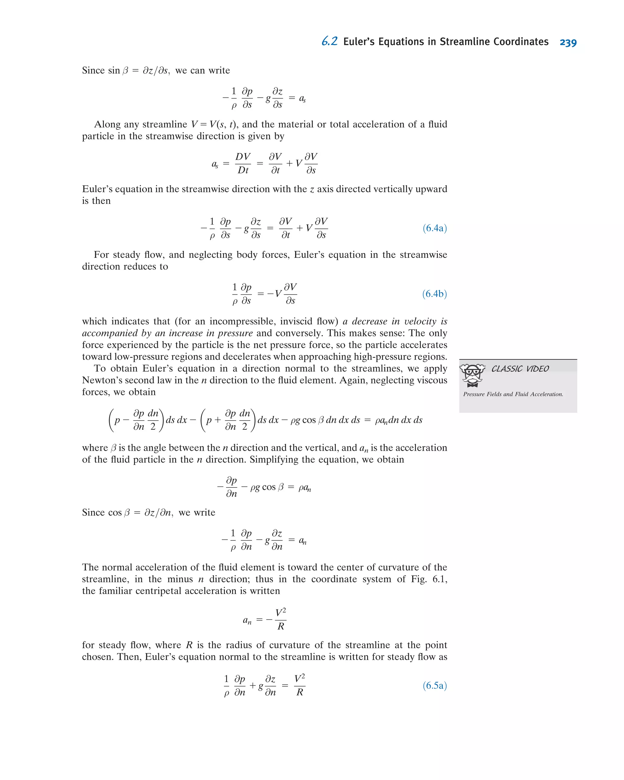

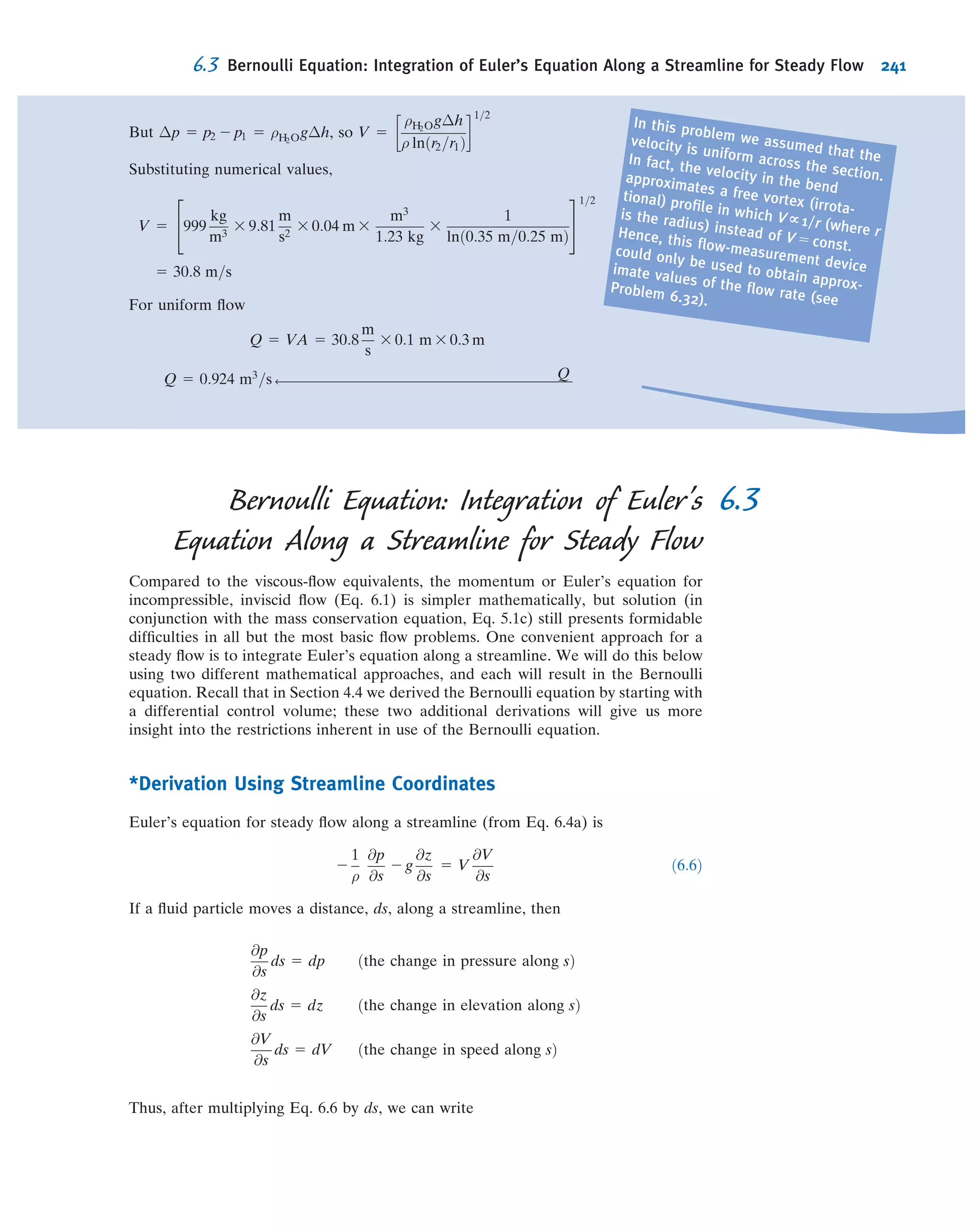

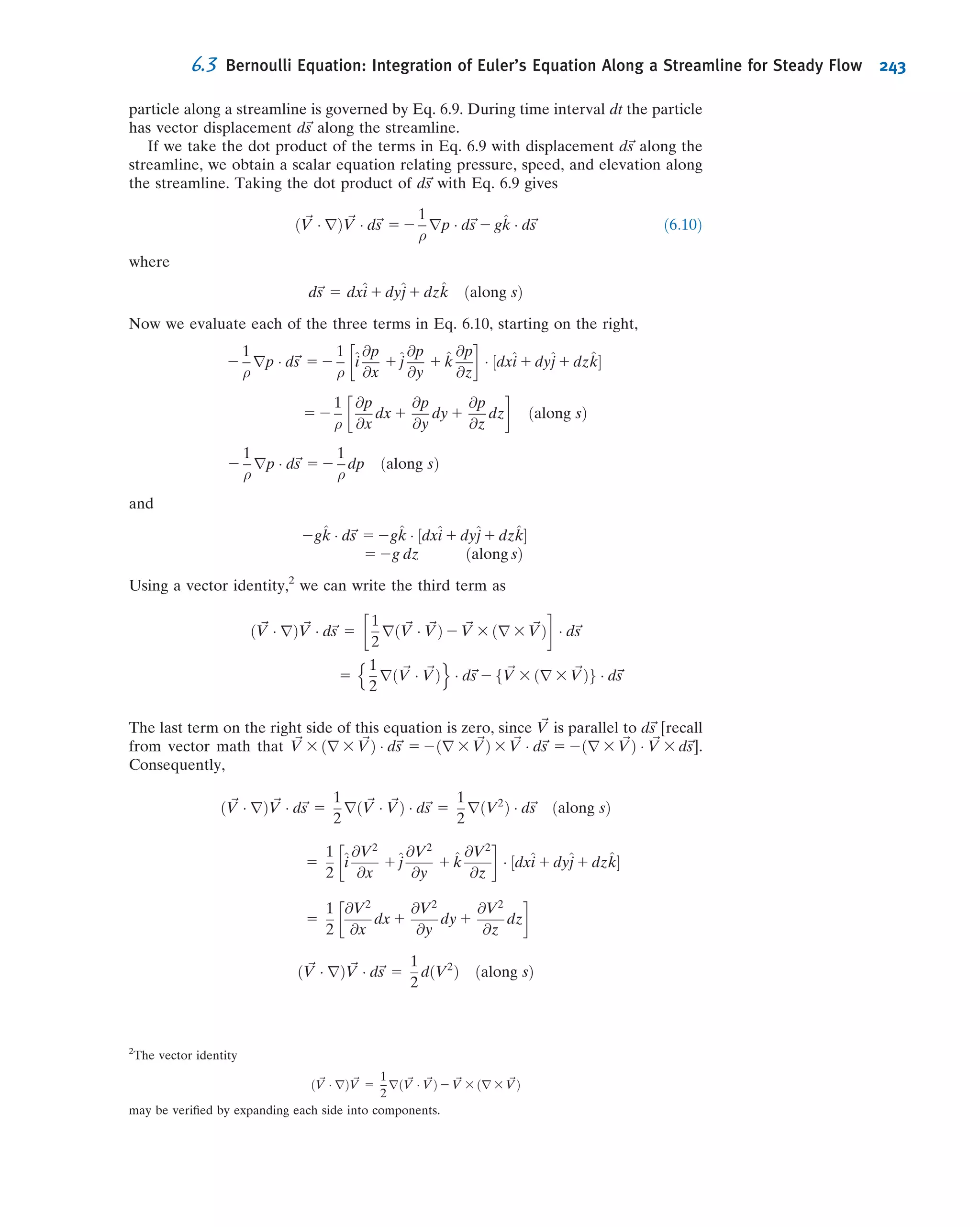
![Equations 5.36 form a system of four simultaneous algebraic equations in the four
unknowns u1, u2, u3, and u4. It’s convenient to write this system in matrix form:
1 0 0 0
21 1 1 Δx 0 0
0 21 1 1 Δx 0
0 0 21 1 1 Δx
2
6
6
4
3
7
7
5
u1
u2
u3
u4
2
6
6
4
3
7
7
5 5
1
0
0
0
2
6
6
4
3
7
7
5 ð5:37Þ
In a general situation (e.g., 2D or 3D domains), we would apply the discrete equations
to the grid points in the interior of the domain. For grid points at or near the
boundary, we would apply a combination of the discrete equations and boundary
conditions. In the end, one would obtain a system of simultaneous algebraic equations
similar to Eqs. 5.36 and a matrix equation similar to Eq. 5.37, with the number of
equations being equal to the number of independent discrete variables. The process is
essentially the same as for the model equation above, with the details obviously being
much more complex.
Solution of Discrete System
The discrete system (Eq. 5.37) for our own simple 1D example can be easily inverted,
using any number of techniques of linear algebra, to obtain the unknowns at the grid
points. For Δx 5 1
3, the solution is
u1 5 1 u2 5
3
4
u3 5
9
16
u4 5
27
64
The exact solution for Eq. 5.31 with m 5 1 is easily shown to be
uexact 5 e2x
Figure 5.18 shows the comparison of the discrete solution obtained on the four-point
grid with the exact solution, using Excel. The error is largest at the right boundary,
where it is equal to 14.7 percent. [It also shows the results using eight points (N 5 8,
Δx 5 1
7) and sixteen points (N 5 16, Δx 5 1
15), which we discuss below.]
In a practical CFD application, we would have thousands, even millions, of
unknowns in the discrete system; if one were to use, say, a Gaussian elimination
procedure to invert the calculations, it would be extremely time-consuming even with
a fast computer. Hence a lot of work has gone into optimizing the matrix inversion in
0.9
0.8
1
0.7
0.6
0.5
0.4
0.3
0.2 0.4 0.6 0.8 10
N = 4
N = 8
N = 16
Exact solution
x
u
Fig. 5.18 Comparison of the numerical solution obtained on three
different grids with the exact solution.
218 Chapter 5 Introduction to Differential Analysis of Fluid Motion](https://image.slidesharecdn.com/foxphilipj-160402150646/75/Fox-Philip-J-Pritchard-8-ed-Mc-Donald-s-Introduction-to-Fluid-Mechanics-wiley-2011-266-2048.jpg)

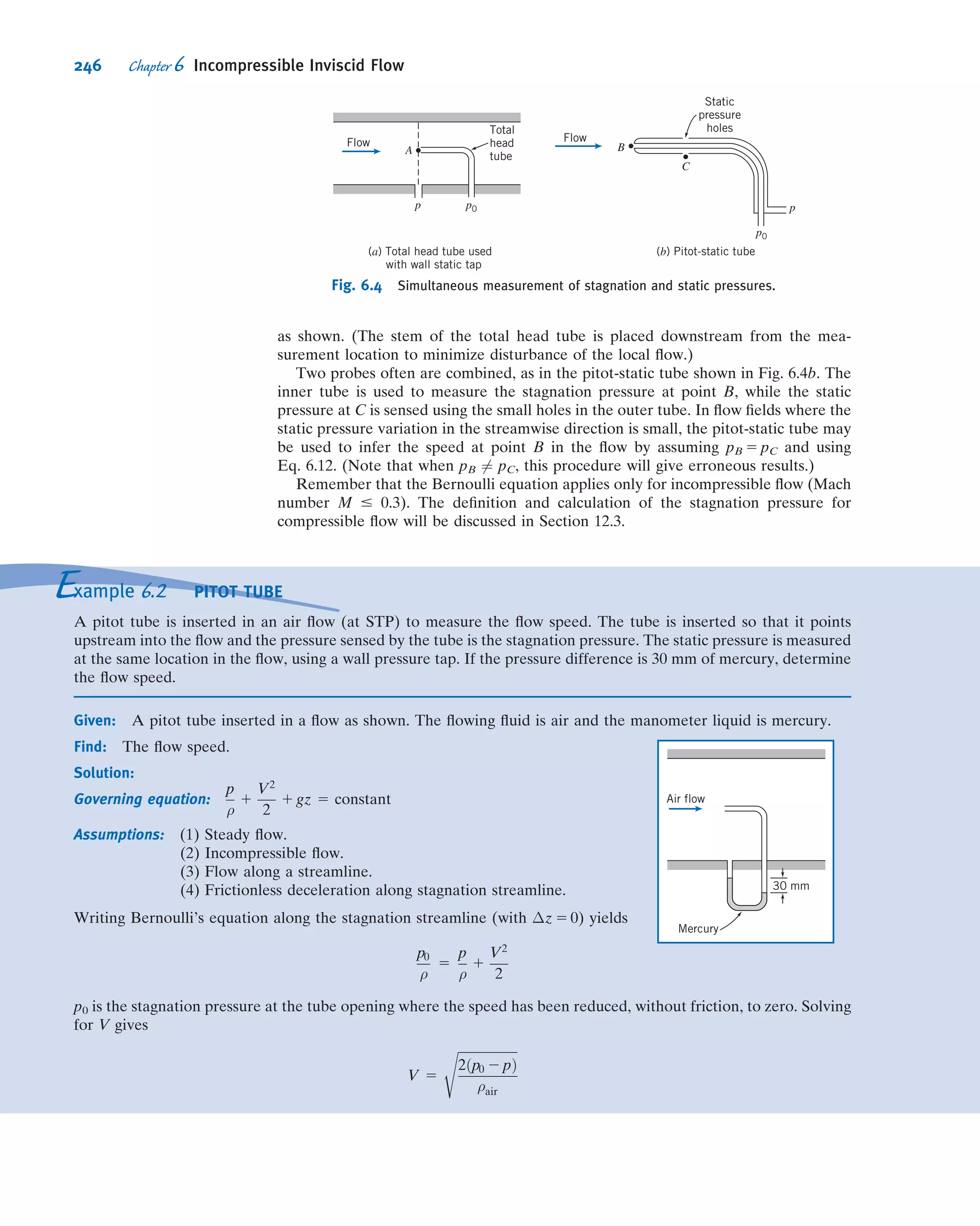
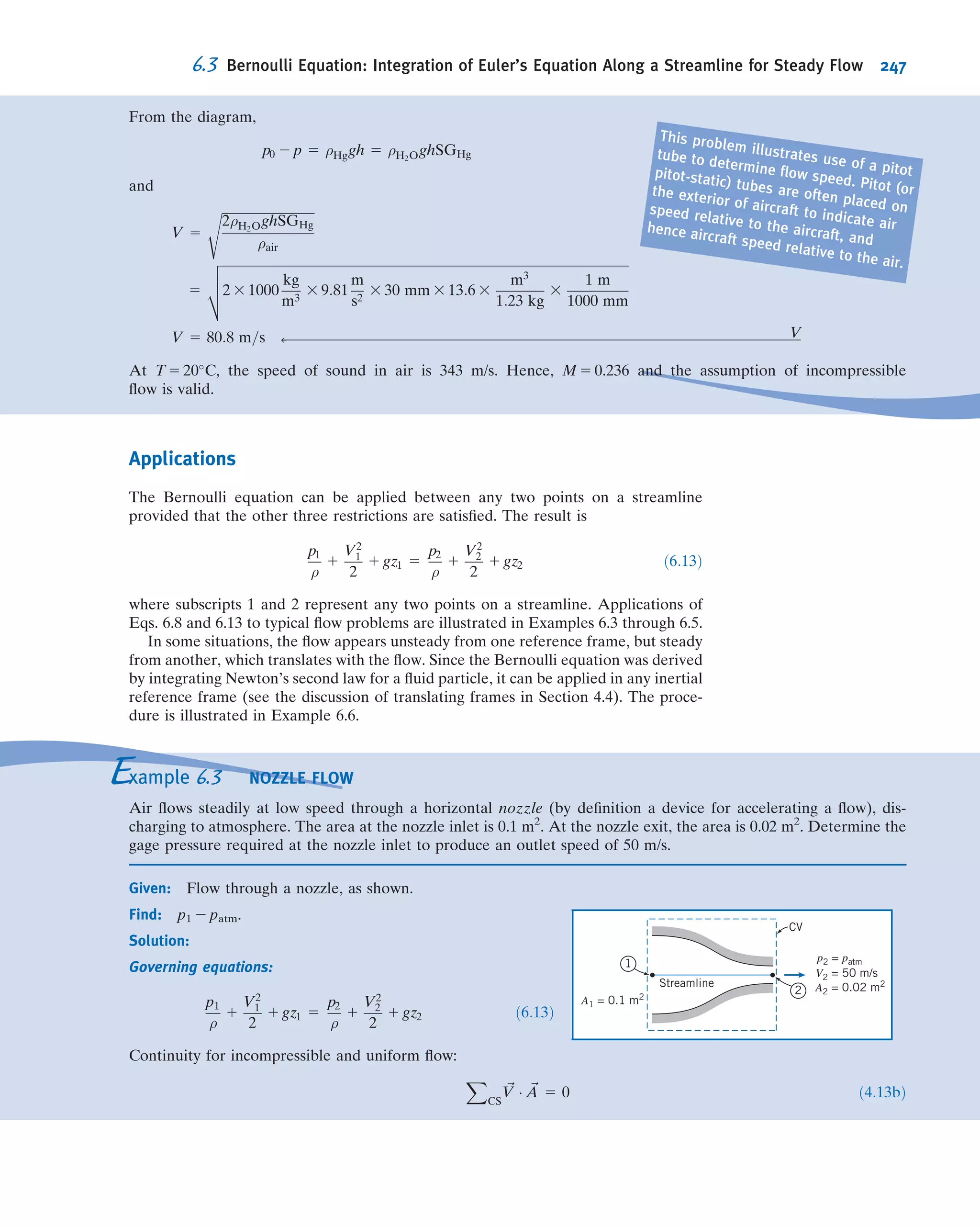

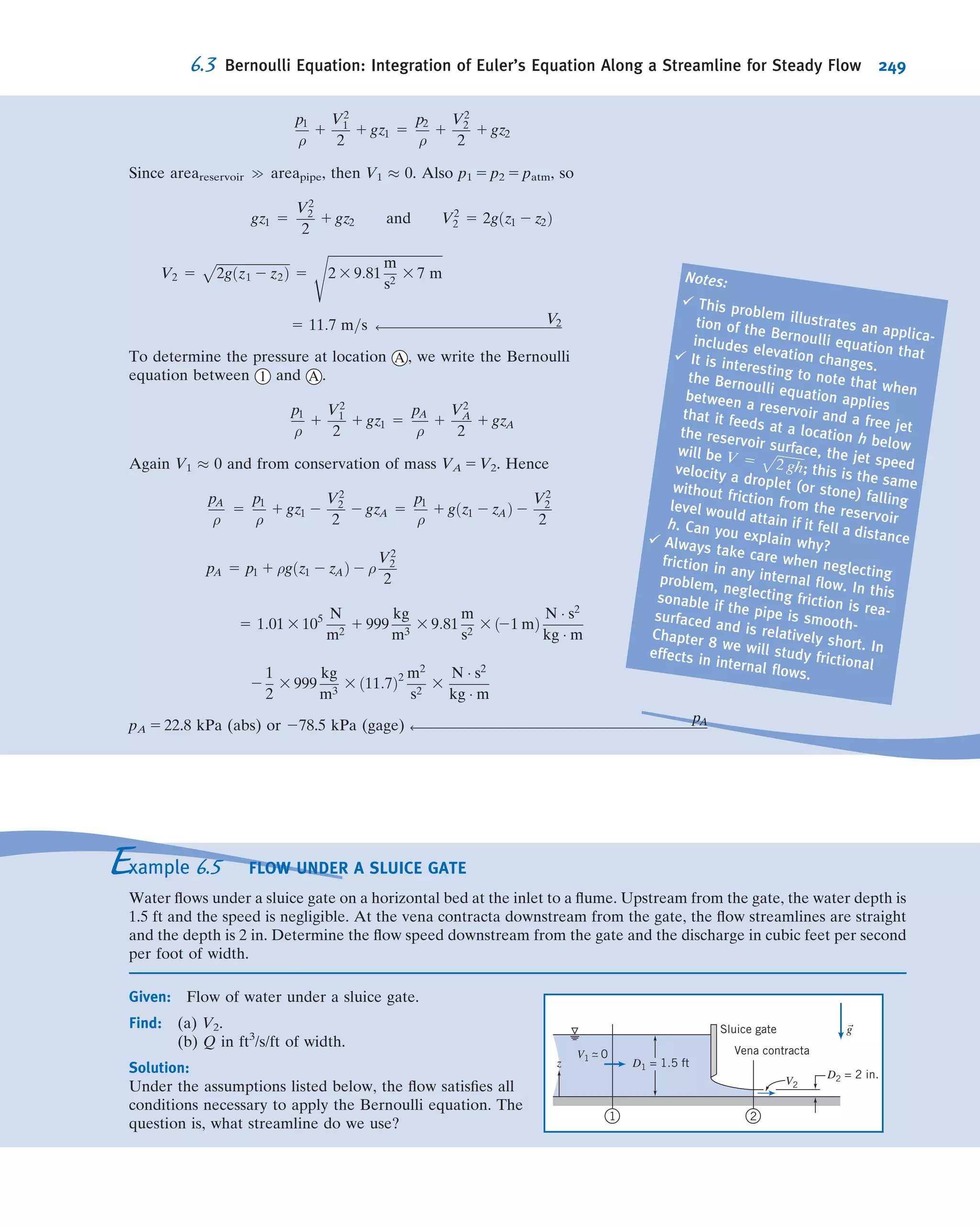
![Many engineering flows are turbulent, characterized by large, nearly random fluc-
tuationsinvelocityand pressureinbothspace andtime.Turbulent flowsoften occurinthe
limit of high Reynolds numbers. For most turbulent flows, it is not possible to resolve
the vast range of time and length scales, even with powerful computers. Instead, one
solves for a statistical average of the flow properties. In order to do this, it is necessary to
augment the governing equations with a turbulence model. Unfortunately, there is no
single turbulence model that is uniformly valid for all flows, so most CFD packages allow
you to choose from among several models. Before you use a turbulence model, you need
to understand its possibilities and limitations for the type of flow being considered.
In this brief introduction we have tried to explain some of the concepts behind CFD.
Because it is so difficult and time consuming to develop CFD code, most engineers
use commercial packages such as Fluent [6] and STAR-CD [7]. This introduction will
have hopefully indicated for you the complexity behind those applications, so that they
are not completely a “black box” of magic tricks.
VIDEO
Fully Turbulent Duct Flow.
5.6 Summary and Useful Equations
In this chapter we have:
ü Derived the differential form of the conservation of mass (continuity) equation in vector form as well as in rectangular and
cylindrical coordinates.
ü *Defined the stream function ψ for a two-dimensional incompressible flow and learned how to derive the velocity components
from it, as well as to find ψ from the velocity field.
ü Learned how to obtain the total, local, and convective accelerations of a fluid particle from the velocity field.
ü Presented examples of fluid particle translation and rotation, and both linear and angular deformation.
ü Defined vorticity and circulation of a flow.
ü Derived, and solved for simple cases, the NavierÀStokes equations, and discussed the physical meaning of each term.
ü *Been introduced to some basis ideas behind computational fluid dynamics.
We have also explored such ideas as how to determine whether a flow is incompressible by using the velocity field
and, given one velocity component of a two-dimensional incompressible flow field, how to derive the other velocity
component.
In this chapter we studied the effects of viscous stresses on fluid particle deformation and rotation; in the next
chapter we examine flows for which viscous effects are negligible.
Note: Most of the Useful Equations in the table below have a number of constraints or limitations—be sure to refer
to their page numbers for details!
Useful Equations
Continuity equation (general, rectan-
gular coordinates):
@ρu
@x
1
@ρv
@y
1
@ρw
@z
1
@ρ
@t
5 0
rÁρ ~V 1
@ρ
@t
5 0
(5.1a)
(5.1b)
Page 175
Continuity equation (incompressible,
rectangular coordinates):
@u
@x
1
@v
@y
1
@w
@z
5 rÁ ~V 5 0
(5.1c) Page 175
Continuity equation (steady, rectangu-
lar coordinates):
@ρu
@x
1
@ρv
@y
1
@ρw
@z
5 rÁρ ~V 5 0
(5.1d) Page 175
Continuity equation (general, cylindri-
cal coordinates):
1
r
@ðrρVrÞ
@r
1
1
r
@ðρVθÞ
@θ
1
@ðρVzÞ
@z
1
@ρ
@t
5 0
rÁρ ~V 1
@ρ
@t
5 0
(5.2a)
(5.1b)
Pages 178
*This section may be omitted without loss of continuity in the text material.
224 Chapter 5 Introduction to Differential Analysis of Fluid Motion](https://image.slidesharecdn.com/foxphilipj-160402150646/75/Fox-Philip-J-Pritchard-8-ed-Mc-Donald-s-Introduction-to-Fluid-Mechanics-wiley-2011-272-2048.jpg)


![and y are measured in feet. Find a possible y component for
steady, incompressible flow. Is it also valid for unsteady,
incompressible flow? Why? How many y components are
possible?
5.4 The three components of velocity in a velocity field are
given by u 5 Ax 1 By 1 Cz, v 5 Dx 1 Ey 1 Fz, and w 5 Gx 1
Hy 1 Jz. Determine the relationship among the coefficients
A through J that is necessary if this is to be a possible
incompressible flow field.
5.5 For a flow in the xy plane, the x component of velocity is
given by u 5 3x2
y 2 y3
. Determine a possible y component
for steady, incompressible flow. Is it also valid for unsteady,
incompressible flow? Why? How many possible y compo-
nents are there?
5.6 The x component of velocity in a steady, incompressible
flow field in the xy plane is u 5 A/x, where A 5 2 m2
/s, and x
is measured in meters. Find the simplest y component of
velocity for this flow field.
5.7 The y component of velocity in a steady, incompressible
flow field in the xy plane is v 5 Axy(x2
2 y2
), where A 5
3 m23
Ás21
and x and y are measured in meters. Find the
simplest x component of velocity for this flow field.
5.8 The y component of velocity in a steady incompressible
flow field in the xy plane is
v 5
2xy
ðx2 1 y2Þ2
Show that the simplest expression for the x component of
velocity is
u 5
1
ðx2 1 y2Þ
2
2y2
ðx2 1 y2Þ2
5.9 The x component of velocity in a steady incompressible
flow field in the xy plane is u 5 Aex/b
cos(y/b), where
A 5 10 m/s, b 5 5 m, and x and y are measured in meters.
Find the simplest y component of velocity for this flow field.
5.10 A crude approximation for the x component of velocity
in an incompressible laminar boundary layer is a linear
variation from u 5 0 at the surface (y 5 0 ) to the freestream
velocity, U, at the boundary-layer edge (y 5 δ). The equation
for the profile is u 5 Uy/δ, where δ 5 cx1/2
and c is a constant.
Show that the simplest expression for the y component of
velocity is v 5 uy/4x. Evaluate the maximum value of the
ratio v/U, at a location where x 5 0.5 m and δ 5 5 mm.
5.11 A useful approximation for the x component of velocity
in an incompressible laminar boundary layer is a parabolic
variation from u 5 0 at the surface (y 5 0) to the freestream
velocity, U, at the edge of the boundary layer (y 5 δ). The
equation for the profile is u/U 5 2(y/δ) 2 (y/δ)2
, where δ 5
cx1/2
and c is a constant. Show that the simplest expression
for the y component of velocity is
v
U
5
δ
x
1
2
y
δ
2
2
1
3
y
δ
3
Plot v/U versus y/δ to find the location of the maximum value of
the ratio v/U. Evaluate the ratio where δ 5 5 mm and x 5 0.5 m.
5.12 A useful approximation for the x component of velocity
in an incompressible laminar boundary layer is a sinusoidal
variation from u 5 0 at the surface (y 5 0) to the freestream
velocity, U, at the edge of the boundary layer (y 5 δ). The
equation for the profile is u 5 U sin(πy/2δ), where δ 5 cx1/2
and c is a constant. Show that the simplest expression for the
y component of velocity is
v
U
5
1
π
δ
x
cos
π
2
y
δ
1
π
2
y
δ
sin
π
2
y
δ
2 1
h i
Plot u/U and v/U versus y/δ, and find the location of the
maximum value of the ratio v/U. Evaluate the ratio where
x 5 0.5 m and δ 5 5 mm.
5.13 A useful approximation for the x component of velocity
in an incompressible laminar boundary layer is a cubic var-
iation from u 5 0 at the surface (y 5 0) to the freestream
velocity, U, at the edge of the boundary layer (y 5 δ). The
equation for the profile is u/U 5 3
2 (y/δ) 2 1
2(y/δ)3
, where
δ 5 cx1/2
and c is a constant. Derive the simplest expression
for v/U, the y component of velocity ratio. Plot u/U and v/U
versus y/δ, and find the location of the maximum value of the
ratio v/U. Evaluate the ratio where δ 5 5 mm and x 5 0.5 m.
5.14 For a flow in the xy plane, the x component of velocity is
given by u 5 Ax2
y2
, where A 5 0.3 m23
Á s21
, and x and y are
measured in meters. Find a possible y component for steady,
incompressible flow. Is it also valid for unsteady, incom-
pressible flow? Why? How many possible y components are
there? Determine the equation of the streamline for the
simplest y component of velocity. Plot the streamlines
through points (1, 4) and (2, 4).
5.15 The y component of velocity in a steady, incompressible
flow field in the xy plane is v 52Bxy3
, where B 5 0.2 m23
Á s21
,
and x and y are measured in meters. Find the simplest x com-
ponent of velocity for this flow field. Find the equation of
the streamlines for thisflow.Plot the streamlines throughpoints
(1, 4) and (2, 4).
5.16 Consider a water stream from a jet of an oscillating lawn
sprinkler. Describe the corresponding pathline and
streakline.
5.17 Derive the differential form of conservation of mass in
rectangular coordinates by expanding the products of density
and the velocity components, ρu, ρv, and ρw, in a Taylor series
about a point O. Show that the result is identical to Eq. 5.1a.
5.18 Which of the following sets of equations represent
possible incompressible flow cases?
(a) Vr 5 U cos θ; Vθ 5 2U sin θ
(b) Vr 52q/2πr; Vθ 5 K/2πr
(c) Vr 5 U cos θ [1 2 (a/r)2
]; Vθ 5 2U sin θ[1 1 (a/r)2
]
5.19 Which of the following sets of equations represent(s)
possible incompressible flow cases?
(a) Vr 5 2K/r; Vθ 5 0
(b) Vr 5 0; Vθ 5 K/r
(c) Vr 5 2K cos θ/r2
; Vθ 5 2K sin θ/r2
5.20 For an incompressible flow in the rθ plane, the r com-
ponent of velocity is given as Vr 5 U cos θ.
(a) Determine a possible θ component of velocity.
(b) How many possible θ components are there?
Problems 227](https://image.slidesharecdn.com/foxphilipj-160402150646/75/Fox-Philip-J-Pritchard-8-ed-Mc-Donald-s-Introduction-to-Fluid-Mechanics-wiley-2011-275-2048.jpg)

![the initial particle position, (x0, y0) at t 5 0. Determine
the time required for a particle to travel from initial position,
(x0, y0) 5 (1
2, 2) to positions ðx; yÞ 5 ð1; 1Þ and ð2; 1
2Þ: Com-
pare the particle accelerations determined by differentiating
f1(t) and f2(t) with those obtained in Problem 5.56.
5.68 Consider the one-dimensional, incompressible flow
through the circular channel shown. The velocity at section
1 is given by U 5 U0 1 U1 sin ωt, where U0 5 20 m/s,
U1 5 2 m/s, and ω 5 0.3 rad/s. The channel dimensions are
L 5 1 m, R1 5 0.2 m, and R2 5 0.1 m. Determine the particle
acceleration at the channel exit. Plot the results as a function
of time over a complete cycle. On the same plot, show the
acceleration at the channel exit if the channel is constant
area, rather than convergent, and explain the difference
between the curves.
L
x2
R2
x1
R1
P5.68
5.69 Which, if any, of the following flow fields are irrotational?
(a) u 5 2x2
1 y2
2 x2
y; v 5 x3
1 x(y2
2 2y)
(b) u 5 2xy 2 x2
1 y; v 5 2xy 2 y2
1 x2
(c) u 5 xt 1 2y; v 5 xt2
2 yt
(d) u 5 (x 1 2y)xt; v 5 2 (2x 1 y)yt
5.70 Expand ð ~V ÁrÞ ~V in cylindrical coordinates by direct
substitution of the velocity vector to obtain the convective
acceleration of a fluid particle. (Recall the hint in footnote 1
on page 178.) Verify the results given in Eqs. 5.12.
5.71 Consider again the sinusoidal velocity profile used to
model the x component of velocity for a boundary layer in
Problem 5.12. Neglect the vertical component of velocity.
Evaluate the circulation around the contour bounded by
x 5 0.4 m, x 5 0.6 m, y 5 0, and y 5 8 mm. What would be the
results of this evaluation if it were performed 0.2 m further
downstream? Assume U 5 0.5 m/s.
5.72 Consider the velocity field for flow in a rectangular
“corner,” ~V 5 Ax^i 2 Ay^j; with A 5 0.3 s21
, as in Example 5.8.
Evaluate the circulation about the unit square of Example 5.8.
5.73 A flow is represented by the velocity field ~V 5 ðx7
2
21x5
y2
1 35x3
y4
2 7xy6
Þ^i 1 ð7x6
y 2 35x4
y3
1 21x2
y5
2 y7
Þ^j.
Determine if the field is (a) a possible incompressible flow
and (b) irrotational.
5.74 Consider the two-dimensional flow field in which u 5 Ax2
and v 5 Bxy, where A 5 1/2 ft21
Ás21
, B 5 21 ft21
Ás21
, and the
coordinates are measured in feet. Show that the velocity field
represents a possible incompressible flow. Determine the
rotation at point (x, y) 5 (1, 1). Evaluate the circulation about
the “curve” bounded by y 5 0, x 5 1, y 5 1, and x 5 0.
5.75 Consider the two-dimensional flow field in which u 5 Axy
and v 5 By2
, where A 5 1m2 1
Ás2 1
; B 5 2 1
2 m2 1
Á s2 1
; and
the coordinates are measured in meters. Show that the velocity
field represents a possible incompressible flow. Determine the
rotation at point (x, y) 5 (1, 1). Evaluate the circulation about
the “curve” bounded by y 5 0, x 5 1, y 5 1, and x 5 0.
*5.76 Consider a flow field represented by the stream function
ψ 5 3x5
y 2 10x3
y3
1 3xy5
. Is this a possible two-dimensional
incompressible flow? Is the flow irrotational?
*5.77 Consider the flow field represented by the stream
function ψ 5 x6
2 15x4
y2
1 15x2
y4
2 y6
. Is this a possible two-
dimensional, incompressible flow? Is the flow irrotational?
*5.78 Consider a velocity field for motion parallel to the x
axis with constant shear. The shear rate is du/dy 5 A, where
A 5 0.1 s21
. Obtain an expression for the velocity field, ~V.
Calculate the rate of rotation. Evaluate the stream function
for this flow field.
*5.79 Consider a flow field represented by the stream function
ψ 52 A/2(x2
1 y2
), where A 5 constant. Is this a possible two-
dimensional incompressible flow? Is the flow irrotational?
*5.80 Consider the flow field represented by the stream func-
tion ψ 5 Axy 1 Ay2
, where A 5 1 s21
. Show that this represents
apossibleincompressibleflowfield.Evaluatetherotationofthe
flow. Plot a few streamlines in the upper half plane.
*5.81 A flow field is represented by the stream function
ψ 5 x2
2 y2
. Find the corresponding velocity field. Show that
this flow field is irrotational. Plot several streamlines and
illustrate the velocity field.
*5.82 Consider the velocity field given by ~V 5 Ax2^i 1 Bxy^j,
where A 5 1 ft21
Ás21
, B 5 22 ft21
Ás21
, and the coordinates
are measured in feet.
(a) Determine the fluid rotation.
(b) Evaluate the circulation about the “curve” bounded by
y 5 0, x 5 1, y 5 1, and x 5 0.
(c) Obtain an expression for the stream function.
(d) Plot several streamlines in the first quadrant.
*5.83 Consider the flow represented by the velocity field
~V 5 ðAy þ BÞ^i þ Ax^j, where A 5 10 s21
, B 5 10 ft/s, and the
coordinates are measured in feet.
(a) Obtain an expression for the stream function.
(b) Plot several streamlines (including the stagnation
streamline) in the first quadrant.
(c) Evaluate the circulation about the “curve” bounded by
y 5 0, x 5 1, y 5 1, and x 5 0.
5.84 Consider again the viscometric flow of Example 5.7.
Evaluate the average rate of rotation of a pair of perpendicular
line segments oriented at 645
from the x axis. Show that this
is the same as in the example.
5.85 Consider the pressure-driven flow between stationary
parallel plates separated by distance b. Coordinate y is mea-
sured from the bottom plate. The velocity field is given by
u 5 U(y/b)[12 (y/b)]. Obtain an expression for the circulation
about a closed contour of heighth and length L. Evaluate when
h 5 b/2 and when h 5 b. Show that the same result is obtained
from the area integral of the Stokes Theorem (Eq. 5.18).
*5.86 The velocity field near the core of a tornado can be
approximated as
*These problems require material from sections that may be omitted without loss of continuity in the text material.
Problems 231](https://image.slidesharecdn.com/foxphilipj-160402150646/75/Fox-Philip-J-Pritchard-8-ed-Mc-Donald-s-Introduction-to-Fluid-Mechanics-wiley-2011-279-2048.jpg)
![~V 5 2
q
2πr
ˆer 1
K
2πr
ˆeθ
Is this an irrotational flow field? Obtain the stream function
for this flow.
5.87 The velocity profile for fully developed flow in a circular
tube is Vz 5 Vmax[1 2 (r/R)2
]. Evaluate the rates of linear and
angular deformation for this flow. Obtain an expression for
the vorticity vector, ~ζ:
5.88 Consider the pressure-driven flow between stationary
parallel plates separated by distance 2b. Coordinate y is
measured from the channel centerline. The velocity field is
given by u 5 umax[1 2 (y/b)2
]. Evaluate the rates of linear and
angular deformation. Obtain an expression for the vorticity
vector, ~ζ: Find the location where the vorticity is a maximum.
Momentum Equation
5.89 Consider a steady, laminar, fully developed, incom-
pressible flow between two infinite plates, as shown. The flow
is due to the motion of the left plate as well a pressure
gradient that is applied in the y direction. Given the condi-
tions that ~V 6¼ ~VðzÞ, w 5 0, and that gravity points in the
negative y direction, prove that u 5 0 and that the pressure
gradient in the y direction must be constant.
V0
x
z
y
P5.89
5.90 Assume the liquid film in Example 5.9 is not isothermal,
but instead has the following distribution:
TðyÞ 5 T0 1 ðTw 2 T0Þ 1 2
y
h
where T0 and Tw are, respectively, the ambient temperature
and the wall temperature. The fluid viscosity decreases with
increasing temperature and is assumed to be described by
μ 5
μ0
1 1 aðT 2 T0Þ
with a . 0. In a manner similar to Example 5.9, derive an
expression for the velocity profile.
5.91 The x component of velocity in a laminar boundary
layer in water is approximated as u 5 U sin(πy/2δ), where
U 5 3 m/s and δ 5 2 mm. The y component of velocity is
much smaller than u. Obtain an expression for the net shear
force per unit volume in the x direction on a fluid element.
Calculate its maximum value for this flow.
5.92 A linear velocity profile was used to model flow in a
laminar incompressible boundary layer in Problem 5.10.
Express the rotation of a fluid particle. Locate the maximum
rate of rotation. Express the rate of angular deformation for a
fluid particle. Locate the maximum rate of angular deforma-
tion. Express the rates of linear deformation for a fluid
particle. Locate the maximum rates of linear deformation.
Express the shear force per unit volume in the x direction.
Locate the maximum shear force per unit volume; interpret
this result.
5.93 Problem 4.35 gave the velocity profile for fully devel-
oped laminar flow in a circular tube as u 5 umax[1 2 (r/R)2
].
Obtain an expression for the shear force per unit volume
in the x direction for this flow. Evaluate its maximum value
for the conditions of Problem 4.35.
5.94 Assume the liquid film in Example 5.9 is horizontal (i.e.,
θ 5 0
) and that the flow is driven by a constant shear stress
on the top surface (y 5 h), τyx 5 C. Assume that the liquid
film is thin enough and flat and that the flow is fully devel-
oped with zero net flow rate (flow rate Q 5 0). Determine the
velocity profile u(y) and the pressure gradient dp/dx.
5.95 Consider a planar microchannel of width h, as shown (it is
actually very long in the x direction and open at both ends).
A Cartesian coordinate system with its origin positioned at the
center of the microchannel is used in the study. The micro-
channel is filled with a weakly conductive solution. When an
electric current is applied across the two conductive walls, the
current density, ~J, transmitted through the solution is parallel
to the y axis. The entire device is placed in a constant magnetic
field, ~B, which is pointed outward from the plane (the z
direction), as shown. Interaction between the current density
and the magnetic field induces a Lorentz force of density
~J 3 ~B. Assume that the conductive solution is incompressible,
and since the sample volume is very small in lab-on-a-chip
applications, the gravitational body force is neglected. Under
steady state, the flow driven by the Lorentz force is described
by the continuity (Eq. 5.1a) and NavierÀStokes equations
(Eqs. 5.27), except the x, y, and z components of the latter have
extra Lorentz force components on the right. Assuming that
the flow is fully developed and the velocity field ~V is a function
of y only, find the three components of velocity.
Conductive wall
J
y
x h
B
Conductive wall
P5.95
5.96 The common thermal polymerase chain reaction (PCR)
process requires the cycling of reagents through three dis-
tinct temperatures for denaturation (90À94
C), annealing
(50À55
C), and extension (72
C). In continuous-flow PCR
reactors, the temperatures of the three thermal zones are
maintained as fixed while the reagents are cycled con-
tinuously through these zones. These temperature variations
induce significant variations in the fluid density, which under
appropriate conditions can be used to generate fluid motion.
The figure depicts a thermosiphon-based PCR device
(Chen et al., 2004, Analytical Chemistry, 76, 3707À3715).
232 Chapter 5 Introduction to Differential Analysis of Fluid Motion](https://image.slidesharecdn.com/foxphilipj-160402150646/75/Fox-Philip-J-Pritchard-8-ed-Mc-Donald-s-Introduction-to-Fluid-Mechanics-wiley-2011-280-2048.jpg)
![The closed loop is filled with PCR reagents. The plan of the
loop is inclined at an angle α with respect to the vertical.
The loop is surrounded by three heaters and coolers that
maintain different temperatures.
(a) Explain why the fluid automatically circulates in the
closed loop along the counterclockwise direction.
(b) What is the effect of the angle α on the fluid velocity?
y
α
50–55°C 90–94°C
72°C
Cooling section
Flow
P5.96
5.97 Electro-osmotic flow (EOF) is the motion of liquid
induced by an applied electric field across a charged capillary
tube or microchannel. Assume the channel wall is negatively
charged, a thin layer called the electric double layer (EDL)
forms in the vicinity of the channel wall in which the number
of positive ions is much larger than that of the negative ions.
The net positively charged ions in the EDL then drag the
electrolyte solution along with them and cause the fluid to
flow toward the cathode. The thickness of the EDL is typically
on the order of 10 nm. When the channel dimensions are
much larger than the thickness of EDL, there is a slip velocity,
y 2
εζ
μ
~E, on the channel wall, where ε is the fluid permittivity,
ζ is the negative surface electric potential, ~E is the electric
field intensity, and μ is the fluid dynamic viscosity. Consider a
microchannel formed by two parallel plates. The walls of the
channel have a negative surface electric potential of ζ. The
microchannel is filled with an electrolyte solution, and the
microchannel ends are subjected to an electric potential dif-
ference that gives rise to a uniform electric field strength of E
along the x direction. The pressure gradient in the channel is
zero. Derive the velocity of the steady, fully developed elec-
tro-osmotic flow. Compare the velocity profile of the EOF to
that of pressure-driven flow. Calculate the EOF velocity using
ε 5 7.08 3 10210
CÁV21
m21
, ζ 5 20.1 V, μ 5 1023
PaÁs, and
E 5 1000 V/m.
Negatively charged wall
y
x
h
E
Anode Cathode
Negatively charged wall
P5.97
Introduction to Computational Fluid Dynamics
*5.98 A tank contains water (20
C) at an initial depth y0 5
1 m. The tank diameter is D 5 250 mm, and a tube of diameter
d 5 3 mm and length L 5 4 m is attached to the bottom of the
tank. For laminar flow a reasonable model for the water level
over time is
dy
dt
5 2
d4
ρg
32D2μL
y yð0Þ 5 y0
Using Euler methods with time steps of 12 min and 6 min:
(a) Estimate the water depth after 120 min, and compute
the errors compared to the exact solution
yexactðtÞ 5 y0e
2
d4
ρg
32D2μL
t
(b) Plot the Euler and exact results.
d
L
D
P5.98
*5.99 Use the Euler method to solve and plot
dy
dx
5 cosðxÞ yð0Þ 5 0
from x 5 0 to x 5 π/2, using step sizes of π/48, π/96, and π/144.
Also plot the exact solution,
yðxÞ 5 sinðxÞ
and compute the errors at x 5 π/2 for the three Euler method
solutions.
*5.100 Use Excel to generate the solution of Eq. 5.31 for m 5 1
shown in Fig. 5.18. To do so, you need to learn how to perform
linear algebra in Excel. For example, for N 5 4 you will end up
with the matrix equation of Eq. 5.37. To solve this equation for
the u values, you will have to compute the inverse of the 4 3 4
matrix, and then multiply this inverse into the 4 3 1 matrix on
the right of the equation. In Excel, to do array operations,
you must use the following rules: Pre-select the cells that will
contain the result; use the appropriate Excel array function
(look at Excel’s Help for details); press Ctrl1Shift1Enter,
not just Enter. For example, to invert the 4 3 4 matrix you
would: Pre-select a blank 4 3 4 array that will contain the
inverse matrix; type5 minverse([array containing matrix to be
inverted]); press Ctrl1Shift1Enter. To multiply a 4 3 4 matrix
into a 4 3 1 matrix you would: Pre-select a blank 4 3 1 array
that will contain the result; type 5 mmult([array containing
4 3 4 matrix], [array containing 4 3 1 matrix]); press
Ctrl1Shift1Enter.
*These problems require material from sections that may be omitted without loss of continuity in the text material.
Problems 233](https://image.slidesharecdn.com/foxphilipj-160402150646/75/Fox-Philip-J-Pritchard-8-ed-Mc-Donald-s-Introduction-to-Fluid-Mechanics-wiley-2011-281-2048.jpg)

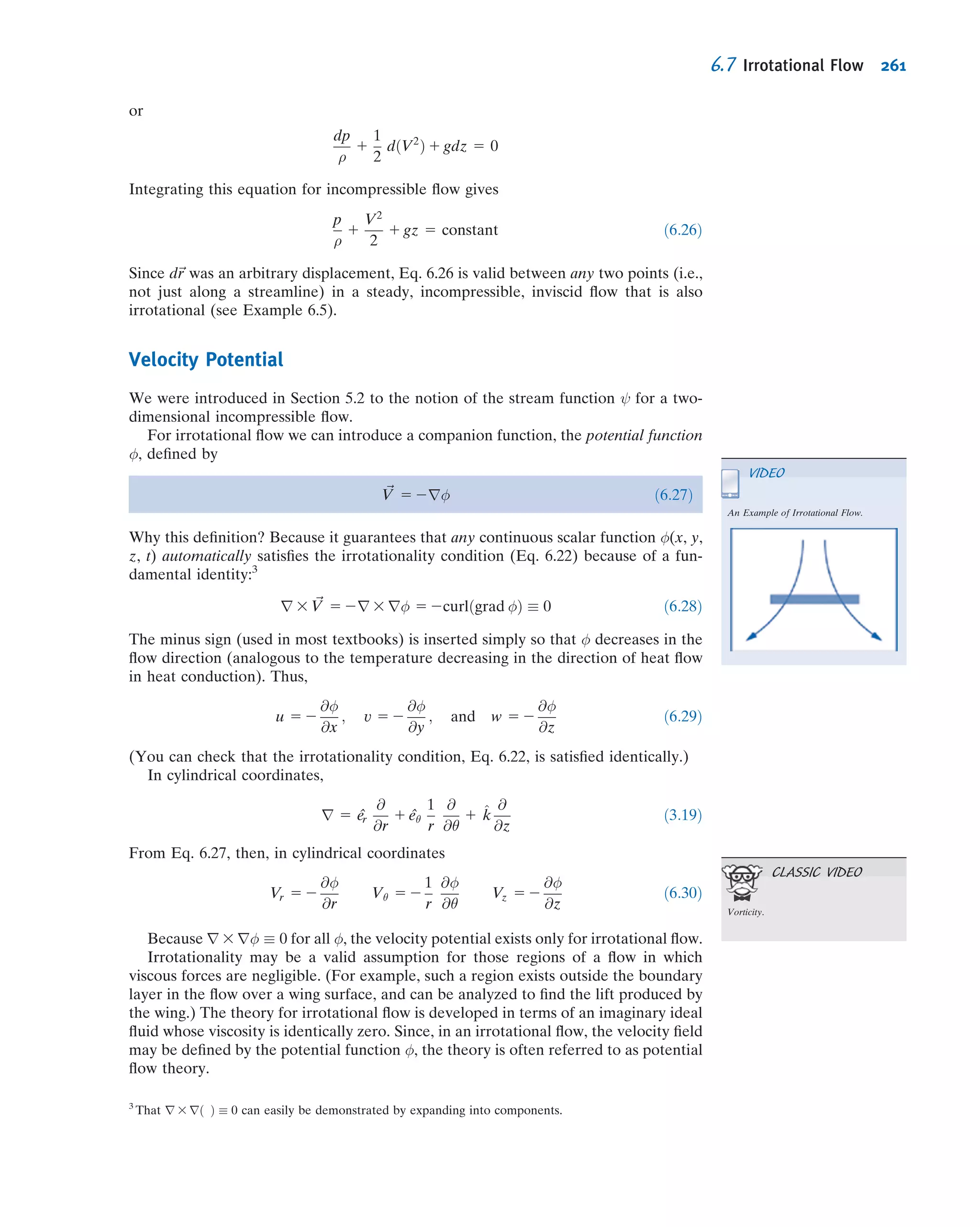


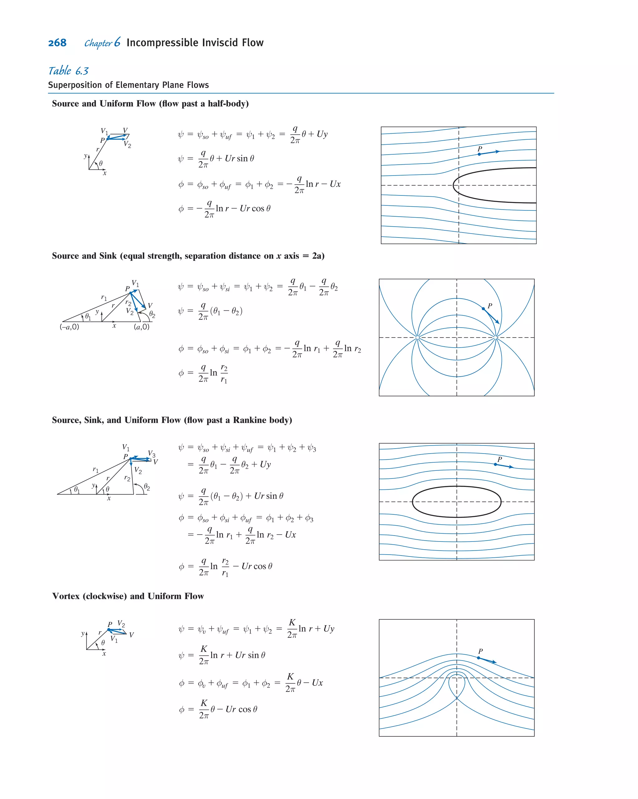
![particle along a streamline is governed by Eq. 6.9. During time interval dt the particle
has vector displacement d~s along the streamline.
If we take the dot product of the terms in Eq. 6.9 with displacement d~s along the
streamline, we obtain a scalar equation relating pressure, speed, and elevation along
the streamline. Taking the dot product of d~s with Eq. 6.9 gives
ð ~V Á rÞ ~V Á d~s 5 2
1
ρ
rp Á d~s 2 g^k Á d~s ð6:10Þ
where
d~s 5 dx^i 1 dy^j 1 dz^k ðalong sÞ
Now we evaluate each of the three terms in Eq. 6.10, starting on the right,
2
1
ρ
rp Á d~s 5 2
1
ρ
^i
@p
@x
1^j
@p
@y
1 ^k
@p
@z
!
Á ½dx^i 1 dy^j 1 dz^kŠ
5 2
1
ρ
@p
@x
dx 1
@p
@y
dy 1
@p
@z
dz
!
ðalong sÞ
2
1
ρ
rp Á d~s 5 2
1
ρ
dp ðalong sÞ
and
2g^k Á d~s 5 2g^k Á ½dx^i 1 dy^j 1 dz^kŠ
5 2g dz ðalong sÞ
Using a vector identity,2
we can write the third term as
ð ~V Á rÞ ~V Á d~s 5
1
2
rð ~V Á ~VÞ 2 ~V 3 ðr 3 ~VÞ
!
Á d~s
5
n 1
2
rð ~V Á ~VÞ
o
Á d~s 2 f ~V 3 ðr 3 ~VÞg Á d~s
The last term on the right side of this equation is zero, since ~V is parallel to d~s [recall
from vector math that ~V 3 ðr 3 ~VÞ Á d~s 5 2ðr 3 ~VÞ 3 ~V Á d~s 5 2ðr 3 ~VÞ Á ~V 3 d~s].
Consequently,
ð ~V Á rÞ ~V Á d~s 5
1
2
rð ~V Á ~VÞ Á d~s 5
1
2
rðV2
Þ Á d~s ðalong sÞ
5
1
2
^i
@V2
@x
1^j
@V2
@y
1 ^k
@V2
@z
!
Á ½dx^i 1 dy^j 1 dz^kŠ
5
1
2
@V2
@x
dx 1
@V2
@y
dy 1
@V2
@z
dz
!
ð ~V Á rÞ ~V Á d~s 5
1
2
dðV2
Þ ðalong sÞ
2
The vector identity
ð ~V Á rÞ ~V 5
1
2
rð ~V Á ~VÞ 2 ~V 3 ðr 3 ~VÞ
may be verified by expanding each side into components.
6.3 Bernoulli Equation: Integration of Euler’s Equation Along a Streamline for Steady Flow 243](https://image.slidesharecdn.com/foxphilipj-160402150646/75/Fox-Philip-J-Pritchard-8-ed-Mc-Donald-s-Introduction-to-Fluid-Mechanics-wiley-2011-291-2048.jpg)
![Substituting these three terms into Eq. 6.10 yields
dp
ρ
1
1
2
dðV2
Þ 1 g dz 5 0 ðalong sÞ
Integrating this equation, we obtain
Z
dp
ρ
1
V2
2
1 gz 5 constant ðalong sÞ
If the density is constant, we obtain the Bernoulli equation
p
ρ
1
V2
2
1 gz 5 constant
As expected, we see that the last two equations are identical to Eqs. 6.7 and 6.8
derived previously using streamline coordinates. The Bernoulli equation, derived
using rectangular coordinates, is still subject to the restrictions: (1) steady flow,
(2) incompressible flow, (3) frictionless flow, and (4) flow along a streamline.
Static, Stagnation, and Dynamic Pressures
The pressure, p, which we have used in deriving the Bernoulli equation, Eq. 6.8, is the
thermodynamic pressure; it is commonly called the static pressure. The static pressure
is the pressure experienced by the fluid particle as it moves (so it is something of a
misnomer!)—we also have the stagnation and dynamic pressures, which we will define
shortly. How do we measure the pressure in a fluid in motion?
In Section 6.2 we showed that there is no pressure variation normal to straight
streamlines. This fact makes it possible to measure the static pressure in a flowing fluid
using a wall pressure “tap,” placed in a region where the flow streamlines are straight,
as shown in Fig. 6.2a. The pressure tap is a small hole, drilled carefully in the wall, with
its axis perpendicular to the surface. If the hole is perpendicular to the duct wall and
free from burrs, accurate measurements of static pressure can be made by connecting
the tap to a suitable pressure-measuring instrument [1].
In a fluid stream far from a wall, or where streamlines are curved, accurate static
pressure measurements can be made by careful use of a static pressure probe, shown
in Fig. 6.2b. Such probes must be designed so that the measuring holes are placed
correctly with respect to the probe tip and stem to avoid erroneous results [2]. In use,
the measuring section must be aligned with the local flow direction. (In these figures, it
may appear that the pressure tap and small holes would allow flow to enter or leave or
otherwise be entrained by the main flow, but each of these is ultimately attached to a
pressure sensor or manometer and is therefore a dead-end, leading to no flow being
possible—see Example 6.2.)
Pressure
tap
Flow
streamlines
(a) Wall pressure tap (b) Static pressure probe
Flow
Small holes
Stem
To manometer or
pressure gage
Fig. 6.2 Measurement of static pressure.
244 Chapter 6 Incompressible Inviscid Flow](https://image.slidesharecdn.com/foxphilipj-160402150646/75/Fox-Philip-J-Pritchard-8-ed-Mc-Donald-s-Introduction-to-Fluid-Mechanics-wiley-2011-292-2048.jpg)
![Static pressure probes, such as that shown in Fig 6.2b, and in a variety of other
forms, are available commercially in sizes as small as 1.5 mm ( 1
16 in.) in diameter [3].
The stagnation pressure is obtained when a flowing fluid is decelerated to zero
speed by a frictionless process. For incompressible flow, the Bernoulli equation can be
used to relate changes in speed and pressure along a streamline for such a process.
Neglecting elevation differences, Eq. 6.8 becomes
p
ρ
1
V2
2
5 constant
If the static pressure is p at a point in the flow where the speed is V, then the stag-
nation pressure, p0, where the stagnation speed, V0, is zero, may be computed from
ϭ 0
p0
ϩ
V0
2
ϭ
p
ϩ
V2
2
2
or
p0 5 p 1
1
2
ρV2
ð6:11Þ
Equation 6.11 is a mathematical statement of the definition of stagnation pressure,
valid for incompressible flow. The term 1
2 ρV2
generally is called the dynamic pressure.
Equation 6.11 states that the stagnation (or total) pressure equals the static pressure
plus the dynamic pressure. One way to picture the three pressures is to imagine you are
standing in a steady wind holding up your hand: The static pressure will be atmo-
spheric pressure; the larger pressure you feel at the center of your hand will be the
stagnation pressure; and the buildup of pressure (the difference between the stagnation
and static pressures) will be the dynamic pressure. Solving Eq. 6.11 for the speed,
V 5
ffiffiffiffiffiffiffiffiffiffiffiffiffiffiffiffiffiffiffi
2ðp0 2 pÞ
ρ
s
ð6:12Þ
Thus, if the stagnation pressure and the static pressure could be measured at a point,
Eq. 6.12 would give the local flow speed.
Stagnation pressure is measured in the laboratory using a probe with a hole that
faces directly upstream as shown in Fig. 6.3. Such a probe is called a stagnation
pressure probe, or pitot (pronounced pea-toe) tube. Again, the measuring section
must be aligned with the local flow direction.
We have seen that static pressure at a point can be measured with a static pressure
tap or probe (Fig. 6.2). If we knew the stagnation pressure at the same point, then
the flow speed could be computed from Eq. 6.12. Two possible experimental setups
are shown in Fig. 6.4.
In Fig. 6.4a, the static pressure corresponding to point A is read from the wall static
pressure tap. The stagnation pressure is measured directly at A by the total head tube,
Flow
To manometer or
pressure gage
Small hole
Fig. 6.3 Measurement of stagnation pressure.
6.3 Bernoulli Equation: Integration of Euler’s Equation Along a Streamline for Steady Flow 245](https://image.slidesharecdn.com/foxphilipj-160402150646/75/Fox-Philip-J-Pritchard-8-ed-Mc-Donald-s-Introduction-to-Fluid-Mechanics-wiley-2011-293-2048.jpg)


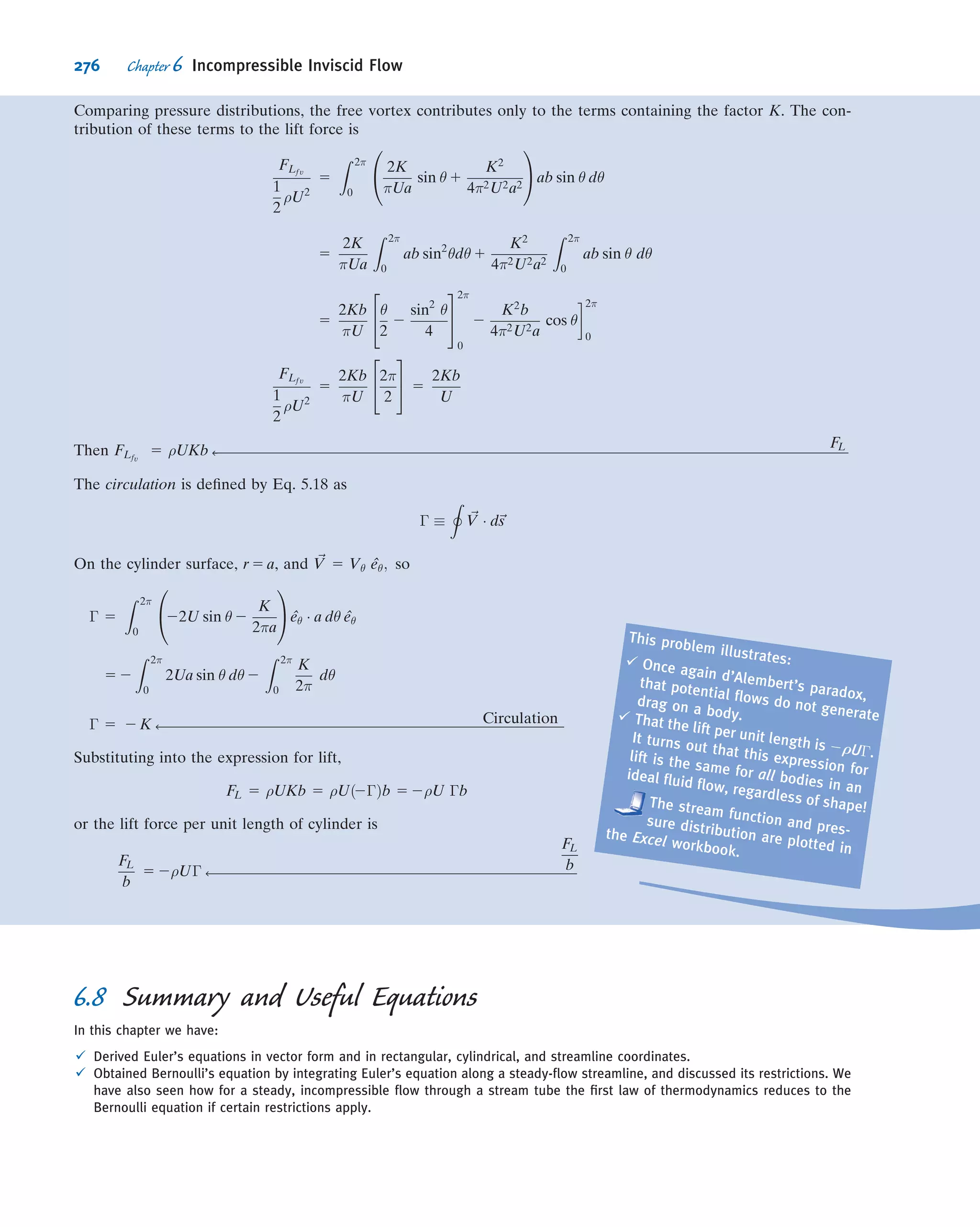
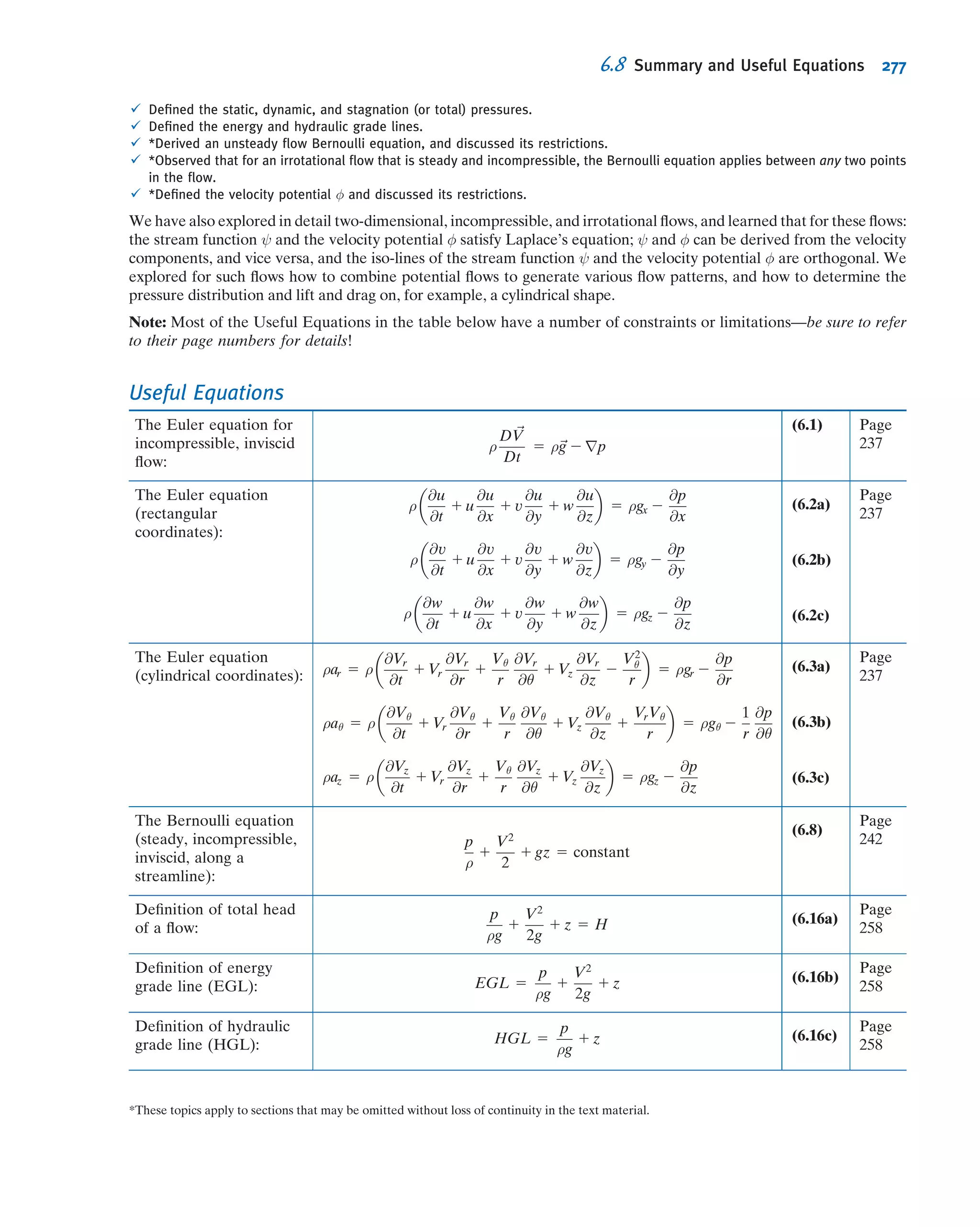
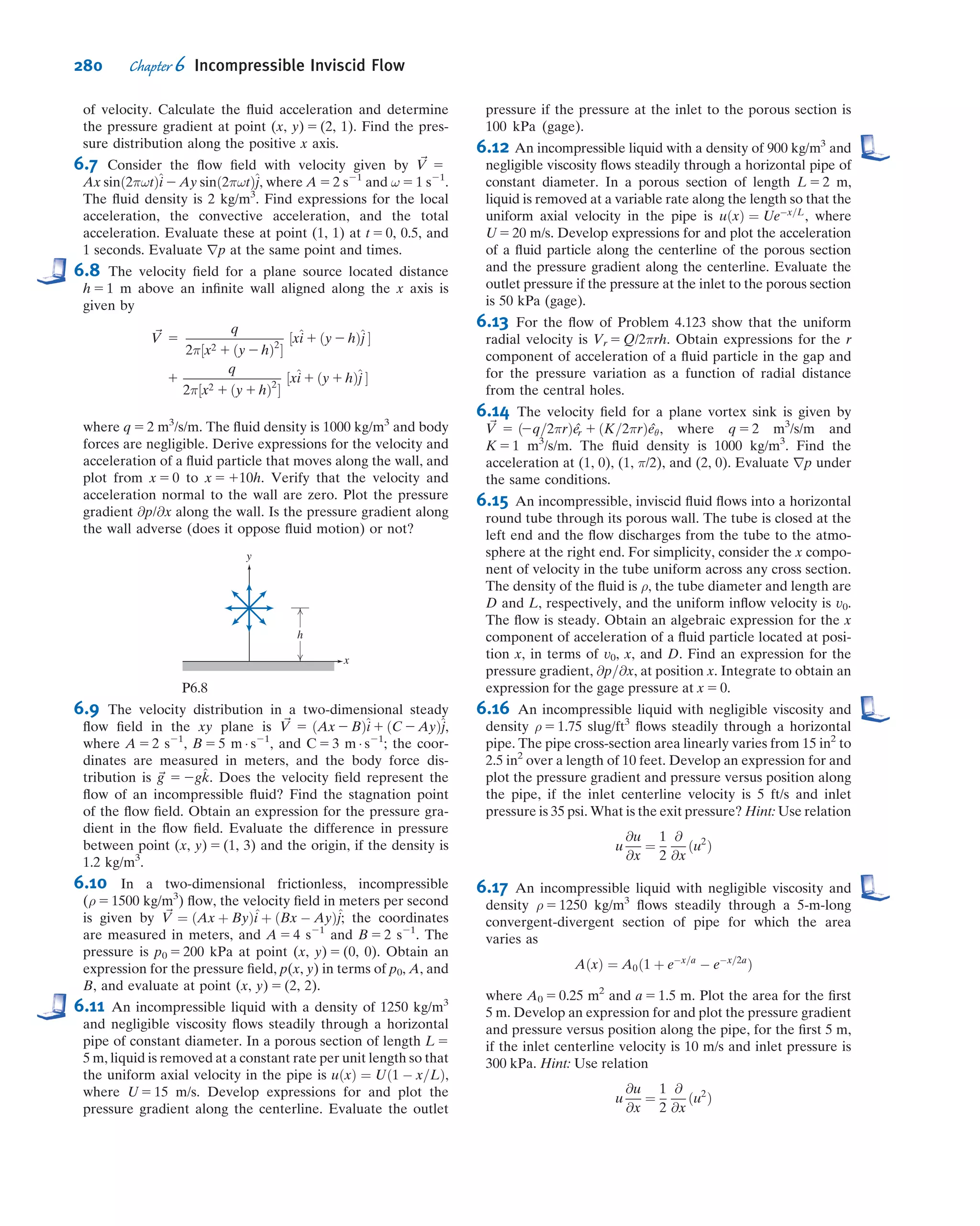
![It looks like we needed restriction (7) to finallytransform the energy equation into the
Bernoulli equation. In fact, we didn’t! It turns out that for an incompressible and fric-
tionless flow [restriction (6), and the fact we are looking only at flows with no shear
forces], restriction (7) is automatically satisfied, as we will demonstrate in Example 6.7.
For the steady, frictionless, and incompressible flow considered in this section, it is
true that the first law of thermodynamics reduces to the Bernoulli equation. Each term
in Eq. 6.15 has dimensions of energy per unit mass (we sometimes refer to the three
terms in the equation as the “pressure” energy, kinetic energy, and potential energy per
unit mass of the fluid). It is not surprising that Eq. 6.15 contains energy terms—after all,
we used the first law of thermodynamics in deriving it. How did we end up with
the same energy-like terms in the Bernoulli equation, which we derived from the
momentum equation? The answer is because we integrated the momentum equation
(which involves force terms) along a streamline (which involves distance), and by doing
so ended up with work or energy terms (work being defined as force times distance):
The work of gravity and pressure forces leads to a kinetic energy change (which came
from integrating momentum over distance). In this context, we can think of the Ber-
noulli equation as a mechanical energy balance—the mechanical energy (“pressure”
plus potential plus kinetic) will be constant. We must always bear in mind that for the
Bernoulli equation to be valid along a streamline requires an incompressible inviscid
flow, in addition to steady flow. It’s interesting that these two properties of the flow—its
compressibility and friction—are what “link” thermodynamic and mechanical energies.
If a fluid is compressible, any flow-induced pressure changes will compress or expand
the fluid, thereby doing work and changing the particle thermal energy; and friction, as
we know from everyday experience, always converts mechanical to thermal energy.
Their absence, therefore, breaks the link between the mechanical and thermal energies,
and they are independent—it’s as if they’re in parallel universes!
Example 6.7 INTERNAL ENERGY AND HEAT TRANSFER IN FRICTIONLESS INCOMPRESSIBLE FLOW
Consider frictionless, incompressible flow with heat transfer. Show that
u2 2 u1 5
δQ
dm
Given: Frictionless, incompressible flow with heat transfer.
Show: u2 2 u1 5
δQ
dm
.
Solution:
In general, internal energy can be expressed as u 5 u(T, v). For incompressible flow, v 5 constant, and u 5 u(T). Thus
the thermodynamic state of the fluid is determined by the single thermodynamic property, T. For any process, the
internal energy change, u2 2 u1, depends only on the temperatures at the end states.
From the Gibbs equation, Tds 5 du 1 ρ dv, valid for a pure substance undergoing any process, we obtain
Tds 5 du
for incompressible flow, since dv 5 0. Since the internal energy change, du, between specified end states, is inde-
pendent of the process, we take a reversible process, for which Tds 5 d(δQ/dm) 5 du. Therefore,
u2 2 u1 5
δQ
dm
ß
6.4 The Bernoulli Equation Interpreted as an Energy Equation 255](https://image.slidesharecdn.com/foxphilipj-160402150646/75/Fox-Philip-J-Pritchard-8-ed-Mc-Donald-s-Introduction-to-Fluid-Mechanics-wiley-2011-303-2048.jpg)
![In summary, when the conditions are satisfied for the Bernoulli equation to be
valid, we can consider separately the mechanical energy and the internal thermal
energy of a fluid particle (this is illustrated in Example 6.8); when they are not
satisfied, there will be an interaction between these energies, the Bernoulli equation
becomes invalid, and we must use the full first law of thermodynamics.
Example 6.8 FRICTIONLESS FLOW WITH HEAT TRANSFER
Water flows steadily from a large open reservoir through a short length of pipe and a nozzle with cross-sectional area
A 5 0.864 in.2
A well-insulated 10 kW heater surrounds the pipe. Find the temperature rise of the water.
Given: Water flows from a large reservoir through the system shown and
discharges to atmospheric pressure. The heater is 10 kW; A4 5 0.864 in.2
Find: The temperature rise of the water between points 1 and 2 .
Solution:
Governing equations:
p
ρ
1
V2
2
1 gz 5 constant ð6:8Þ
X
CS
~V Á ~A 5 0 ð4:13bÞ
ϩ gz) V и dA
V2
2
Q Ϫ Ws Ϫ Wshear ϭ
CV
e dV ϩ
CS
(u ϩ pv ϩ
ϭ 0(4) ϭ 0(4) ϭ 0(1)
͵ ͵t
ð4:56Þ
Assumptions: (1) Steady flow.
(2) Frictionless flow.
(3) Incompressible flow.
(4) No shaft work, no shear work.
(5) Flow along a streamline.
(6) Uniform flow at each section [a consequence of assumption (2)].
Under the assumptions listed, the first law of thermodynamics for the CV shown becomes
_Q 5
Z
CS
u 1 pv 1
V2
2
1 gz
ρ ~V Á d ~A
5
Z
A1
u 1 pv 1
V2
2
1 gz
ρ ~V Á d ~A 1
Z
A2
u 1 pv 1
V2
2
1 gz
ρ ~V Á d ~A
For uniform properties at 1 and 2
_Q 5 2ðρV1A1Þ u1 1 p1v 1
V2
1
2
1 gz1
1 ðρV2A2Þ u2 1 p2v 1
V2
2
2
1 gz2
From conservation of mass, ρV1A1 5 ρV2A2 5 Ám; so
_Q 5 Ám u2 2 u1 1
p2
ρ
1
V2
2
2
1 gz2
2
p1
ρ
1
V2
1
2
1 gz1
!
1
3
2
4
10 ft
Heater
CV
256 Chapter 6 Incompressible Inviscid Flow](https://image.slidesharecdn.com/foxphilipj-160402150646/75/Fox-Philip-J-Pritchard-8-ed-Mc-Donald-s-Introduction-to-Fluid-Mechanics-wiley-2011-304-2048.jpg)

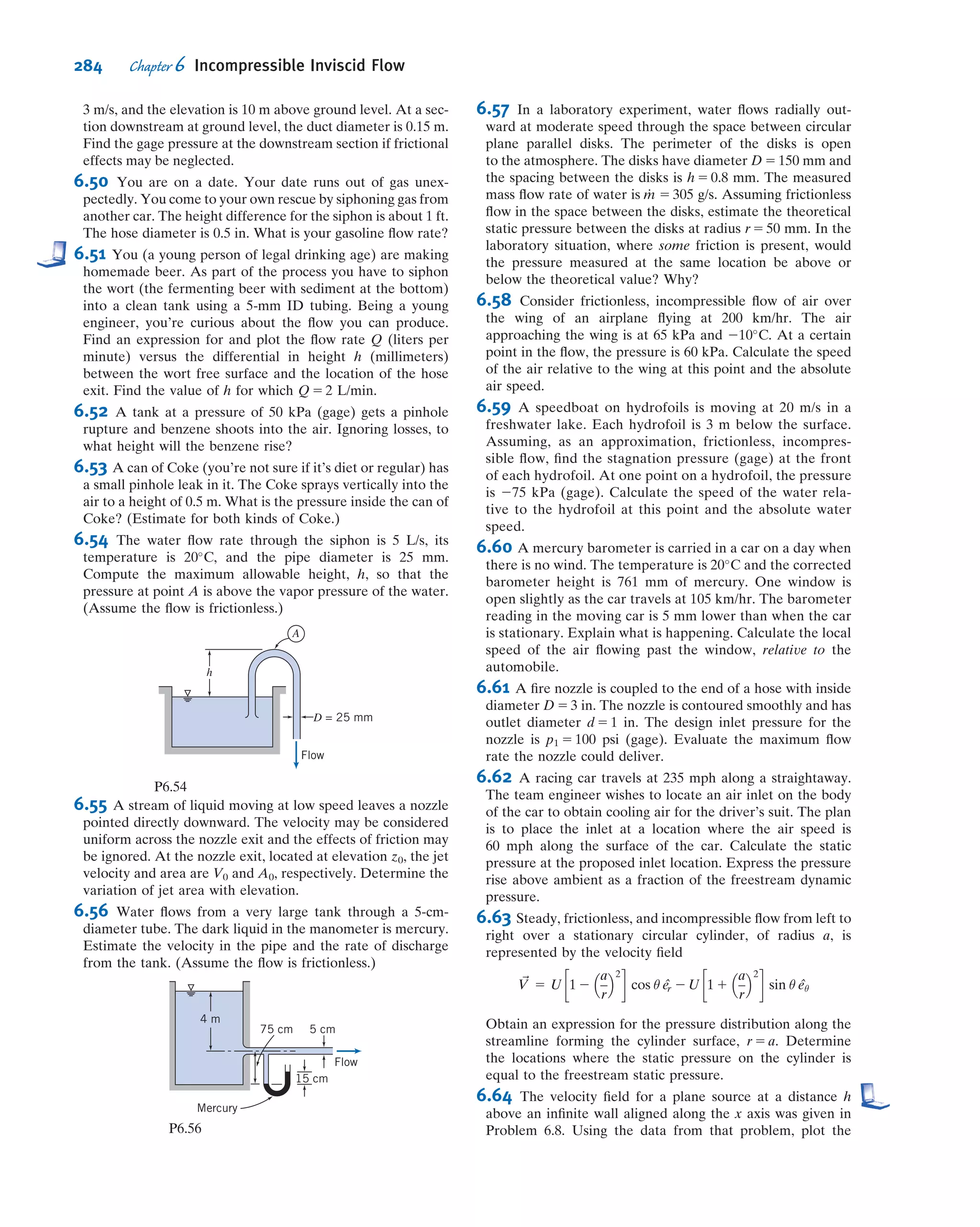
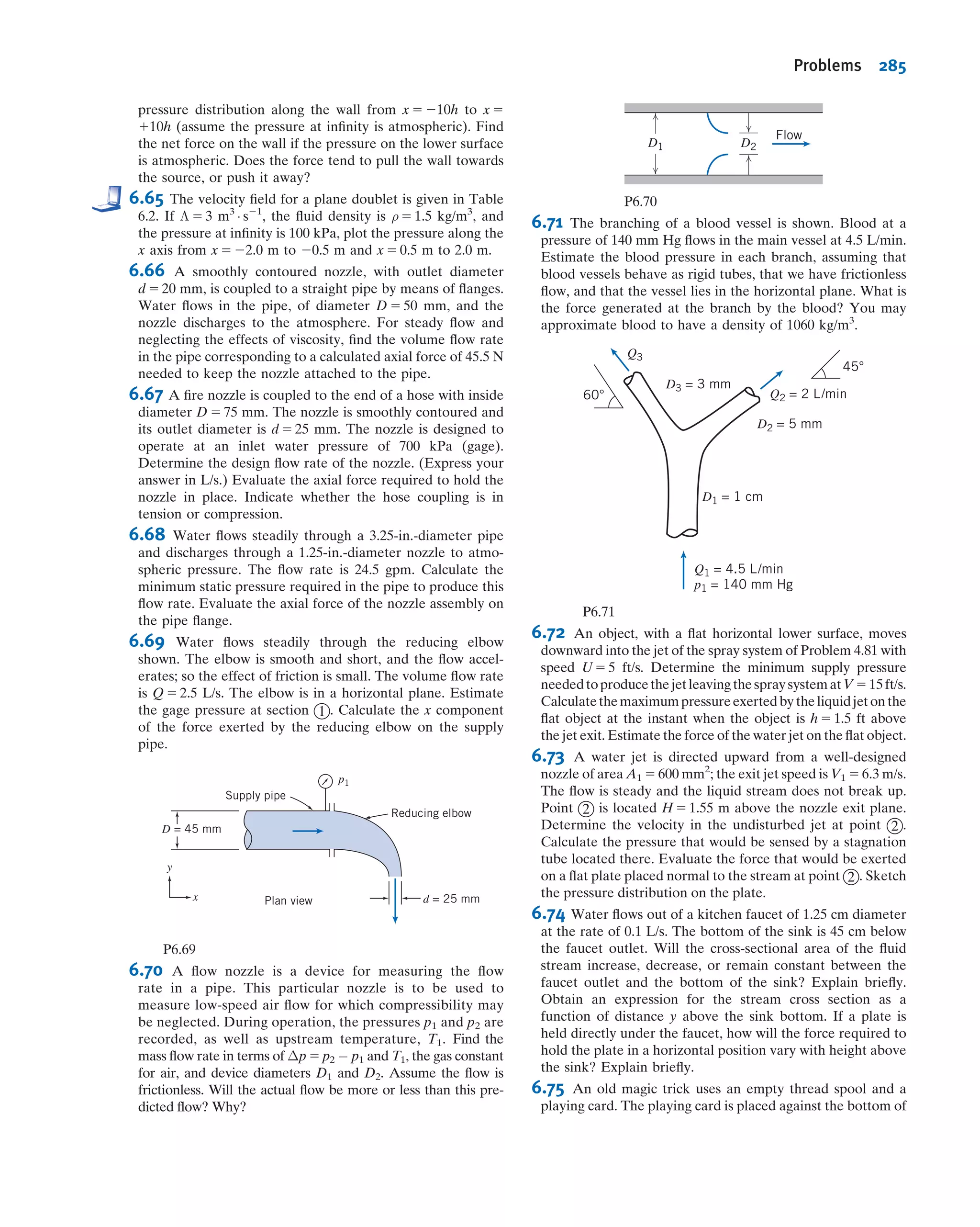


![All real fluids possess viscosity, but there are many situations in which the
assumption of inviscid flow considerably simplifies the analysis and, at the same time,
gives meaningful results. Because of its relative simplicity and mathematical beauty,
potential flow has been studied extensively.4
Stream Function and Velocity Potential for Two-Dimensional,
Irrotational, Incompressible Flow: Laplace’s Equation
For a two-dimensional, incompressible, irrotational flow we have expressions for the
velocity components, u and v, in terms of both the stream function ψ, and the velocity
potential φ,
u 5
@ψ
@y
v 5 2
@ψ
@x
ð5:4Þ
u 5 2
@φ
@x
v 5 2
@φ
@y
ð6:29Þ
Substituting for u and v from Eq. 5.4 into the irrotationality condition,
@v
@x
2
@u
@y
5 0 ð6:23Þ
we obtain
@2
ψ
@x2
1
@2
ψ
@y2
5 r2
ψ 5 0 ð6:31Þ
Substituting for u and v from Eq. 6.29 into the continuity equation,
@u
@x
1
@v
@y
5 0 ð5:3Þ
we obtain
@2
φ
@x2
1
@2
φ
@y2
5 r2
φ 5 0 ð6:32Þ
Equations 6.31 and 6.32 are forms of Laplace’s equation—an equation that arises in
many areas of the physical sciences and engineering. Any function ψ or φ that satisfies
Laplace’s equation represents a possible two-dimensional, incompressible, irrota-
tional flow field.
Table 6.1 summarizes the results of our discussion of the stream function and
velocity potential for two dimensional flows.
The same rules (of when incompressibility and irrotationality apply, and with the
appropriate form of Laplace’s equation) are valid for the stream function and velocity
potential when expressed in cylindrical coordinates,
Vr 5
1
r
@ψ
@θ
and Vθ 5 2
@ψ
@r
ð5:8Þ
4
Anyone interested in a detailed study of potential flow theory may find [4À6] of interest.
262 Chapter 6 Incompressible Inviscid Flow](https://image.slidesharecdn.com/foxphilipj-160402150646/75/Fox-Philip-J-Pritchard-8-ed-Mc-Donald-s-Introduction-to-Fluid-Mechanics-wiley-2011-310-2048.jpg)


![streamline patterns to see where we have regions of high or low velocity and hence
low or high pressure, is very useful. We will examine these last two flows in Examples
6.11 and 6.12. The last example in Table 6.3, the vortex pair, hints at a way to create
flows that simulate the presence of a wall or walls: for the y axis to be a stream-
line (and thus a wall), simply make sure that any objects (e.g., a source, a vortex) in
the positive x quadrants have mirror-image objects in the negative x quadrants; the y
axis will thus be a line of symmetry. For a flow pattern in a 90
corner, we need to
place objects so that we have symmetry with respect to both the x and y axes. For flow
in a corner whose angle is a fraction of 90
(e.g., 30
), we need to place objects in a
radially symmetric fashion.
Because Laplace’s equation appears in many engineering and physics applications,
it has been extensively studied. We saw in Example 5.12 that Laplace’s equation is
sometimes amenable to a fairly simple numerical solution using a spreadsheet. For
analytic solutions, one approach is to use conformal mapping with complex notation.
It turns out that any continuous complex function f(z) (where z 5 x 1 iy, and
i 5
ffiffiffiffiffiffi
21
p
) is a solution of Laplace’s equation, and can therefore represent both φ
and ψ. With this approach many elegant mathematical results have been derived
[7À10]. We mention only two: the circle theorem, which enables any given flow [e.g.,
from a source at some point (a, b)] to be easily transformed to allow for the presence
of a cylinder at the origin; and the Schwarz-Christoffel theorem, which enables a given
flow to be transformed to allow for the presence of virtually unlimited stepwise linear
boundaries (e.g., the presence on the x axis of the silhouette of a building).
Table 6.3
Superposition of Elementary Plane Flows (Continued )
Sink and Vortex
y
x
r
V P
V1
V2
θ
ψ 5 ψsi 1 ψv 5 ψ1 1 ψ2 5 2
q
2π
θ 2
K
2π
ln r
φ 5 φsi 1 φv 5 φ1 1 φ2 5
q
2π
ln r 2
K
2π
θ
P
Vortex Pair (equal strength, opposite rotation, separation distance on x axis 5 2a)
y
x
r2
r1
1
V1
V2
PV
θ 2θ
(a,0)(–a,0)
ψ 5 ψv1 1 ψv2 5 ψ1 1 ψ2 5 2
K
2π
ln r1 1
K
2π
ln r2
ψ 5
K
2π
ln
r2
r1
φ 5 φv1 1 φv2 5 φ1 1 φ2 5 2
K
2π
θ1 1
K
2π
θ2
φ 5
K
2π
ðθ2 2 θ1Þ
P
270 Chapter 6 Incompressible Inviscid Flow](https://image.slidesharecdn.com/foxphilipj-160402150646/75/Fox-Philip-J-Pritchard-8-ed-Mc-Donald-s-Introduction-to-Fluid-Mechanics-wiley-2011-318-2048.jpg)
![Much of this analytical work was done centuries ago, when it was called “hydro-
dynamics” instead of potential theory. A list of famous contributors includes Ber-
noulli, Lagrange, d’Alembert, Cauchy, Rankine, and Euler [11]. As we discussed in
Section 2.6, the theory immediately ran into difficulties: In an ideal fluid flow no body
experiences drag—the d’Alembert paradox of 1752—a result completely counter
to experience. Prandtl, in 1904, resolved this discrepancy by describing how real flows
may be essentially inviscid almost everywhere, but there is always a “boundary layer”
adjacent to the body. In this layer significant viscous effects occur, and the no-slip
condition is satisfied (in potential flow theory the no-slip condition is not satisfied).
Development of this concept, and the Wright brothers’ historic first human flight, led
to rapid developments in aeronautics starting in the 1900s. We will study boundary
layers in detail in Chapter 9, where we will see that their existence leads to drag on
bodies, and also affects the lift of bodies.
An alternative superposition approach is the inverse method in which distributions
of objects such as sources, sinks, and vortices are used to model a body [12]. It is called
inverse because the body shape is deduced based on a desired pressure distribution.
Both the direct and inverse methods, including three-dimensional space, are today
mostly analyzed using computer applications such as Fluent [13] and STAR-CD [14].
Example 6.11 FLOW OVER A CYLINDER: SUPERPOSITION OF DOUBLET AND UNIFORM FLOW
For two-dimensional, incompressible, irrotational flow, the superposition of a doublet and a uniform flow represents
flow around a circular cylinder. Obtain the stream function and velocity potential for this flow pattern. Find the
velocity field, locate the stagnation points and the cylinder surface, and obtain the surface pressure distribution.
Integrate the pressure distribution to obtain the drag and lift forces on the circular cylinder.
Given: Two-dimensional, incompressible, irrotational flow formed from superposition of a doublet and
a uniform flow.
Find: (a) Stream function and velocity potential.
(b) Velocity field.
(c) Stagnation points.
(d) Cylinder surface.
(e) Surface pressure distribution.
(f) Drag force on the circular cylinder.
(g) Lift force on the circular cylinder.
Solution: Stream functions may be added because the flow field is incompressible and irrotational. Thus from Table
6.2, the stream function for the combination is
ψ 5 ψd 1 ψuf 5 2
Λ sin θ
r
1 Ur sin θ ß
ψ
The velocity potential is
φ 5 φd 1 φuf 5 2
Λ cos θ
r
2 Ur cos θ ß
φ
The corresponding velocity components are obtained using Eqs. 6.30 as
Vr 5 2
@φ
@r
5 2
Λ cos θ
r2
1 U cos θ
Vθ 5 2
1
r
@φ
@θ
5 2
Λ sin θ
r2
2 U sin θ
6.7 Irrotational Flow 271](https://image.slidesharecdn.com/foxphilipj-160402150646/75/Fox-Philip-J-Pritchard-8-ed-Mc-Donald-s-Introduction-to-Fluid-Mechanics-wiley-2011-319-2048.jpg)


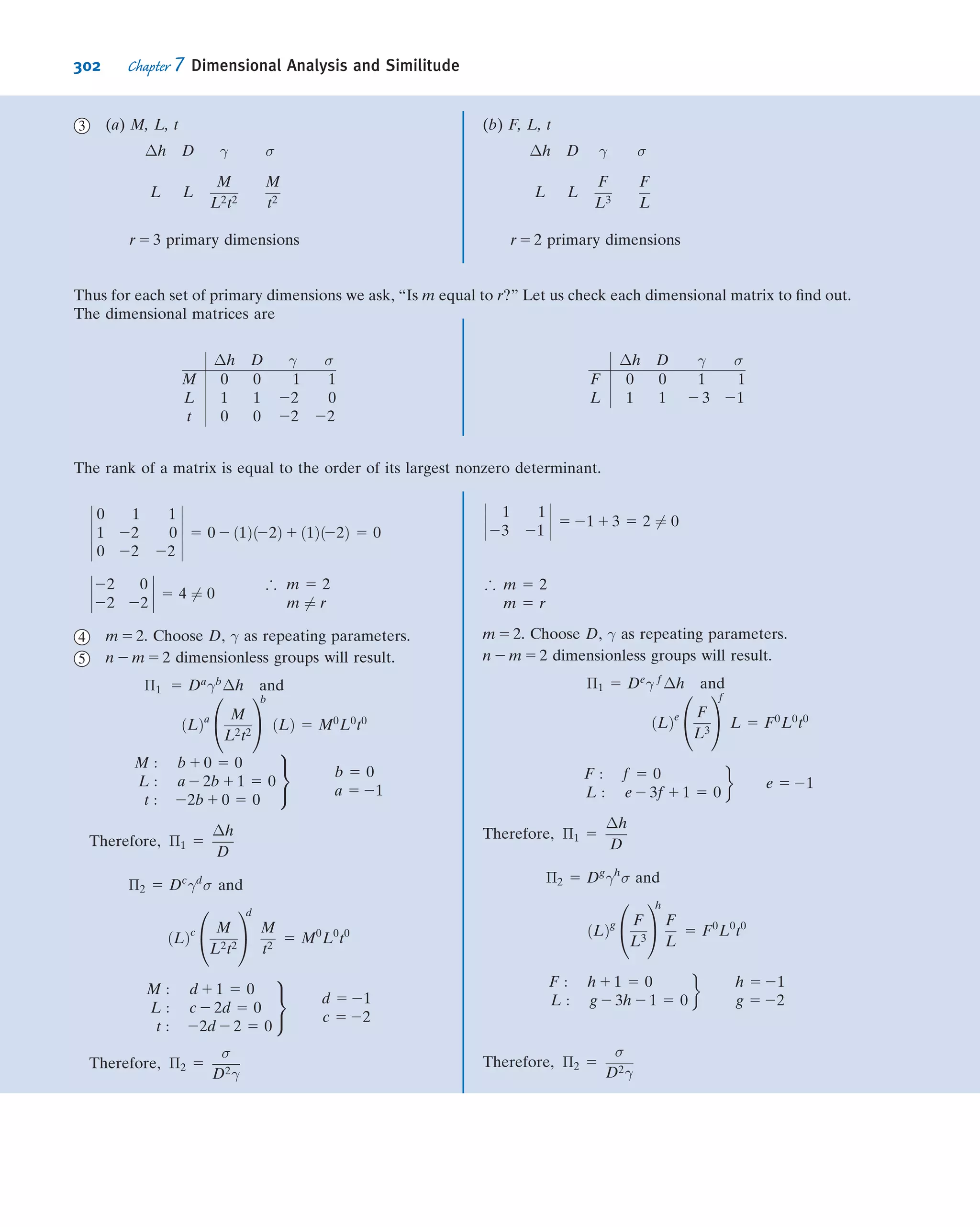
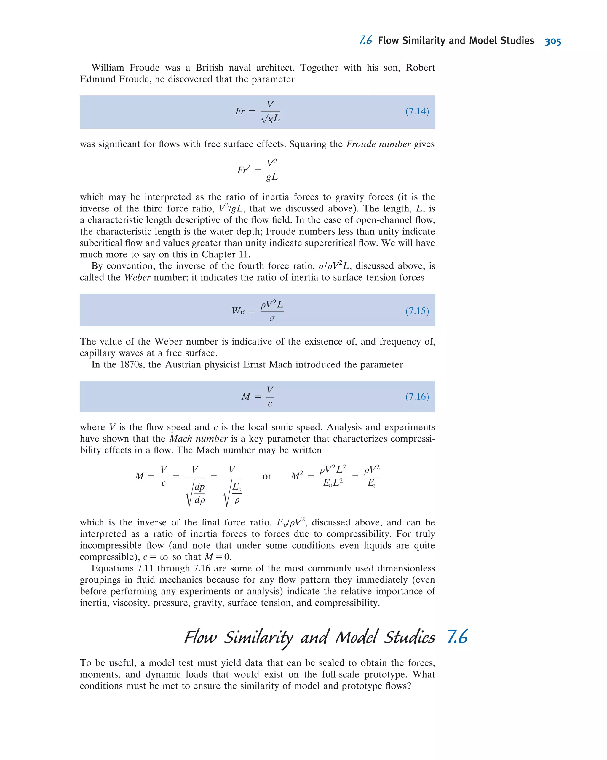
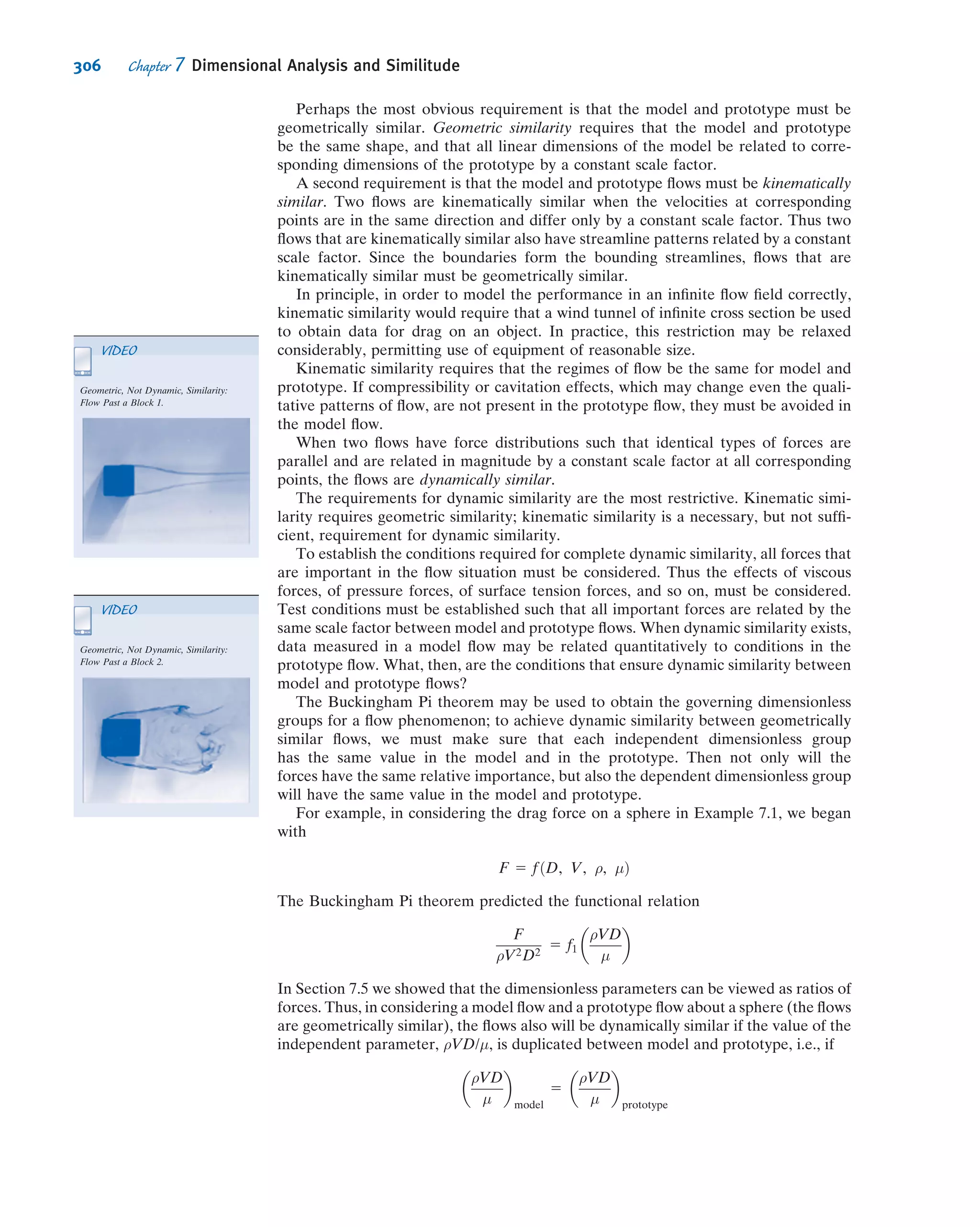

![streamline passing through this point. Plot the streamline
and show both the velocity vector and the acceleration vec-
tor on the plot. (Assume the simplest form of the x compo-
nent of velocity.)
6.27 Consider the velocity field ~V 5 A[x4
2 6x2
y2
1 y4
]^i 1 B
[x3
y 2 xy3
]^j; A 5 2 m23
Á s21
, B is a constant, and the coor-
dinates are measured in meters. Find B for this to be an
incompressible flow. Obtain the equation of the streamline
through point (x, y) 5 (1, 2). Derive an algebraic expression
for the acceleration of a fluid particle. Estimate the radius of
curvature of the streamline at (x, y) 5 (1, 2).
6.28 The velocity field for a plane doublet is given in Table 6.2.
Find an expression for the pressure gradient at any point (r, θ).
6.29 Air flow over a stationary circular cylinder of radius a is
modeled as a steady, frictionless, and incompressible flow
from right to left, given by the velocity field
~V ¼ U
a
r
2
À 1
!
cos θ ^er þ U
a
r
2
þ 1
!
sin θ ^eθ
Consider flow along the streamline forming the cylinder
surface, r 5 a. Express the components of the pressure gra-
dient in terms of angle θ. Obtain an expression for the var-
iation of pressure (gage) on the surface of the cylinder. For
U 5 75 m/s and a 5 150 mm, plot the pressure distribution
(gage) and explain, and find the minimum pressure. Plot the
speed V as a function of r along the radial line θ 5 π/2 for
r . a (that is, directly above the cylinder), and explain.
6.30 To model the velocity distribution in the curved inlet
section of a water channel, the radius of curvature of the
streamlines is expressed as R 5 LR0/2y. As an approximation,
assume the water speed along each streamline is V 5 10 m/s.
Find an expression for and plot the pressure distribution from
y 5 0 to the tunnel wall at y 5 L/2, if the centerline pressure
(gage) is 50 kPa, L 5 75 mm, and R0 5 0.2 m. Find the value of
V for which the wall static pressure becomes 35 kPa.
R
R0
y
x
L___
2
P6.30
6.31 Air at 20 psia and 100
F flows around a smooth corner
at the inlet to a diffuser. The air speed is 150 ft/s, and the
radius of curvature of the streamlines is 3 in. Determine
the magnitude of the centripetal acceleration experienced by
a fluid particle rounding the corner. Express your answer in
gs. Evaluate the pressure gradient, @p/@r.
6.32 Repeat Example 6.1, but with the somewhat more
realistic assumption that the flow is similar to a free vortex
(irrotational) profile, Vθ 5 c/r (where c is a constant), as
shown in Fig. P6.32. In doing so, prove that the flow rate is
given by Q 5 k
ffiffiffiffiffiffiffi
Δp
p
, where k is
k 5 w ln
r2
r1
ffiffiffiffiffiffiffiffiffiffiffiffiffiffiffiffiffiffiffiffi
2r2
2r2
1
ρðr2
2 2 r2
1Þ
s
and w is the depth of the bend.
r1
Vθ
θ
r2
P6.32
6.33 The velocity field in a two-dimensional, steady, inviscid
flow field in the horizontal xy plane is given by
~V 5 ðAx 1 BÞ^i 2 Ay^j, where A 5 1 s21
and B 5 2 m/s; x and
y are measured in meters. Show that streamlines for this flow
are given by (x 1 B/A)y 5 constant. Plot streamlines passing
through points (x, y) 5 (1, 1), (1, 2), and (2, 2). At point
(x, y) 5 (1, 2), evaluate and plot the acceleration vector and
the velocity vector. Find the component of acceleration
along the streamline at the same point; express it as a vector.
Evaluate the pressure gradient along the streamline at the
same point if the fluid is air. What statement, if any, can you
make about the relative value of the pressure at points (1, 1)
and (2, 2)?
6.34 Using the analyses of Example 6.1 and Problem 6.32,
plot the discrepancy (percent) between the flow rates
obtained from assuming uniform flow and the free vortex
(irrotational) profile as a function of inner radius r1.
6.35 The x component of velocity in a two-dimensional,
incompressible flow field is given by u 5 Ax2
; the coordi-
nates are measured in feet and A 5 1 ft21
Á s21
. There is no
velocity component or variation in the z direction. Calcu-
late the acceleration of a fluid particle at point (x, y) 5 (1,
2). Estimate the radius of curvature of the streamline
passing through this point. Plot the streamline and show
both the velocity vector and the acceleration vector on the
plot. (Assume the simplest form of the y component of
velocity.)
6.36 The x component of velocity in a two-dimensional
incompressible flow field is given by u 5 2Λðx2
2 y2
Þ=
ðx2
1 y2
Þ2
, where u is in m/s, the coordinates are measured in
meters, and Λ 5 2 m3
Á s21
. Show that the simplest form of the
y component of velocity is given by v 5 22Λxy=ðx2
1 y2
Þ2
.
There is no velocity component or variation in the z direc-
tion. Calculate the acceleration of fluid particles at points
(x, y) 5 (0, 1), (0, 2), and (0, 3). Estimate the radius of cur-
vature of the streamlines passing through these points. What
does the relation among the three points and their radii of
curvature suggest to you about the flow field? Verify this by
282 Chapter 6 Incompressible Inviscid Flow](https://image.slidesharecdn.com/foxphilipj-160402150646/75/Fox-Philip-J-Pritchard-8-ed-Mc-Donald-s-Introduction-to-Fluid-Mechanics-wiley-2011-330-2048.jpg)
![plotting these streamlines. [Hint: You will need to use an
integrating factor.]
6.37 The x component of velocity in a two-dimensional,
incompressible flow field is given by u 5 Axy; the coordi-
nates are measured in meters and A 5 2 m21
Á s21
. There is
no velocity component or variation in the z direction.
Calculate the acceleration of a fluid particle at point
(x, y) 5 (2, 1). Estimate the radius of curvature of the
streamline passing through this point. Plot the streamline
and show both the velocity vector and the acceleration
vector on the plot. (Assume the simplest form of the y
component of velocity.)
The Bernoulli Equation
6.38 Water flows at a speed of 25 ft/s. Calculate the dynamic
pressure of this flow. Express your answer in inches of
mercury.
6.39 Calculate the dynamic pressure that corresponds to a
speed of 100 km/hr in standard air. Express your answer in
millimeters of water.
6.40 Plot the speed of air versus the dynamic pressure
(in millimeters of mercury), up to a dynamic pressure of
250 mm Hg.
6.41 You present your open hand out of the window of an
automobile perpendicular to the airflow. Assuming for sim-
plicity that the air pressure on the entire front surface is
stagnation pressure (with respect to automobile coordi-
nates), with atmospheric pressure on the rear surface, esti-
mate the net force on your hand when driving at (a) 30 mph
and (b) 60 mph. Do these results roughly correspond with
your experience? Do the simplifications tend to make the
calculated force an over- or underestimate?
6.42 A jet of air from a nozzle is blown at right angles
against a wall in which two pressure taps are located. A
manometer connected to the tap directly in front of the
jet shows a head of 25 mm of mercury above atmospheric.
Determine the approximate speed of the air leaving the
nozzle if it is at 210
C and 200 kPa. At the second tap
a manometer indicates a head of 5 mm of mercury
above atmospheric; what is the approximate speed of the air
there?
6.43 A pitot-static tube is used to measure the speed of air at
standard conditions at a point in a flow. To ensure that the
flow may be assumed incompressible for calculations of
engineering accuracy, the speed is to be maintained at 100
m/s or less. Determine the manometer deflection, in milli-
meters of water, that corresponds to the maximum desirable
speed.
6.44 The inlet contraction and test section of a laboratory
wind tunnel are shown. The air speed in the test section is
U 5 50 m/s. A total-head tube pointed upstream indicates
that the stagnation pressure on the test section centerline is
10 mm of water below atmospheric. The laboratory is main-
tained at atmospheric pressure and a temperature of 25
C.
Evaluate the dynamic pressure on the centerline of the wind
tunnel test section. Compute the static pressure at the same
point. Qualitatively compare the static pressure at the tunnel
wall with that at the centerline. Explain why the two may not
be identical.
Contraction
Test section
U = 50 m/sFlow
P6.44
6.45 Maintenance work on high-pressure hydraulic systems
requires special precautions. A small leak can result in a high-
speed jet of hydraulic fluid that can penetrate the skin and
cause serious injury (therefore troubleshooters are cautioned
to use a piece of paper or cardboard, not a finger, to search for
leaks). Calculate and plot the jet speed of a leak versus system
pressure, for pressures up to 40 MPa (gage). Explain how a
high-speed jet of hydraulic fluid can cause injury.
6.46 An open-circuit wind tunnel draws in air from the
atmosphere through a well-contoured nozzle. In the test
section, where the flow is straight and nearly uniform, a static
pressure tap is drilled into the tunnel wall. A manometer
connected to the tap shows that static pressure within the
tunnel is 45 mm of water below atmospheric. Assume that
the air is incompressible, and at 25
C, 100 kPa (abs). Cal-
culate the air speed in the wind-tunnel test section.
6.47 The wheeled cart shown in Problem 4.128 rolls with
negligible resistance. The cart is to accelerate to the right.
The jet speed is V 5 40 m/s. The jet area remains constant at
A 5 25 mm2
. Neglect viscous forces between the water and
vane. When the cart attains speed U 5 15 m/s, calculate the
stagnation pressure of the water leaving the nozzle with
respect to a fixed observer, the stagnation pressure of the
water jet leaving the nozzle with respect to an observer on
the vane, the absolute velocity of the jet leaving the vane
with respect to a fixed observer, and the stagnation pressure
of the jet leaving the vane with respect to a fixed observer.
How would viscous forces affect the latter stagnation pres-
sure, i.e., would viscous forces increase, decrease, or leave
unchanged this stagnation pressure? Justify your answer.
6.48 Water flows steadily up the vertical 1-in.-diameter pipe
and out the nozzle, which is 0.5 in. in diameter, discharging to
atmospheric pressure. The stream velocity at the nozzle exit
must be 30 ft/s. Calculate the minimum gage pressure
required at section 1 . If the device were inverted, what
would be the required minimum pressure at section 1 to
maintain the nozzle exit velocity at 30 ft/s?
2
1
Flow
10 ft
V2
P6.48
6.49 Water flows in a circular duct. At one section the diam-
eter is 0.3 m, the static pressure is 260 kPa(gage), the velocity is
Problems 283](https://image.slidesharecdn.com/foxphilipj-160402150646/75/Fox-Philip-J-Pritchard-8-ed-Mc-Donald-s-Introduction-to-Fluid-Mechanics-wiley-2011-331-2048.jpg)
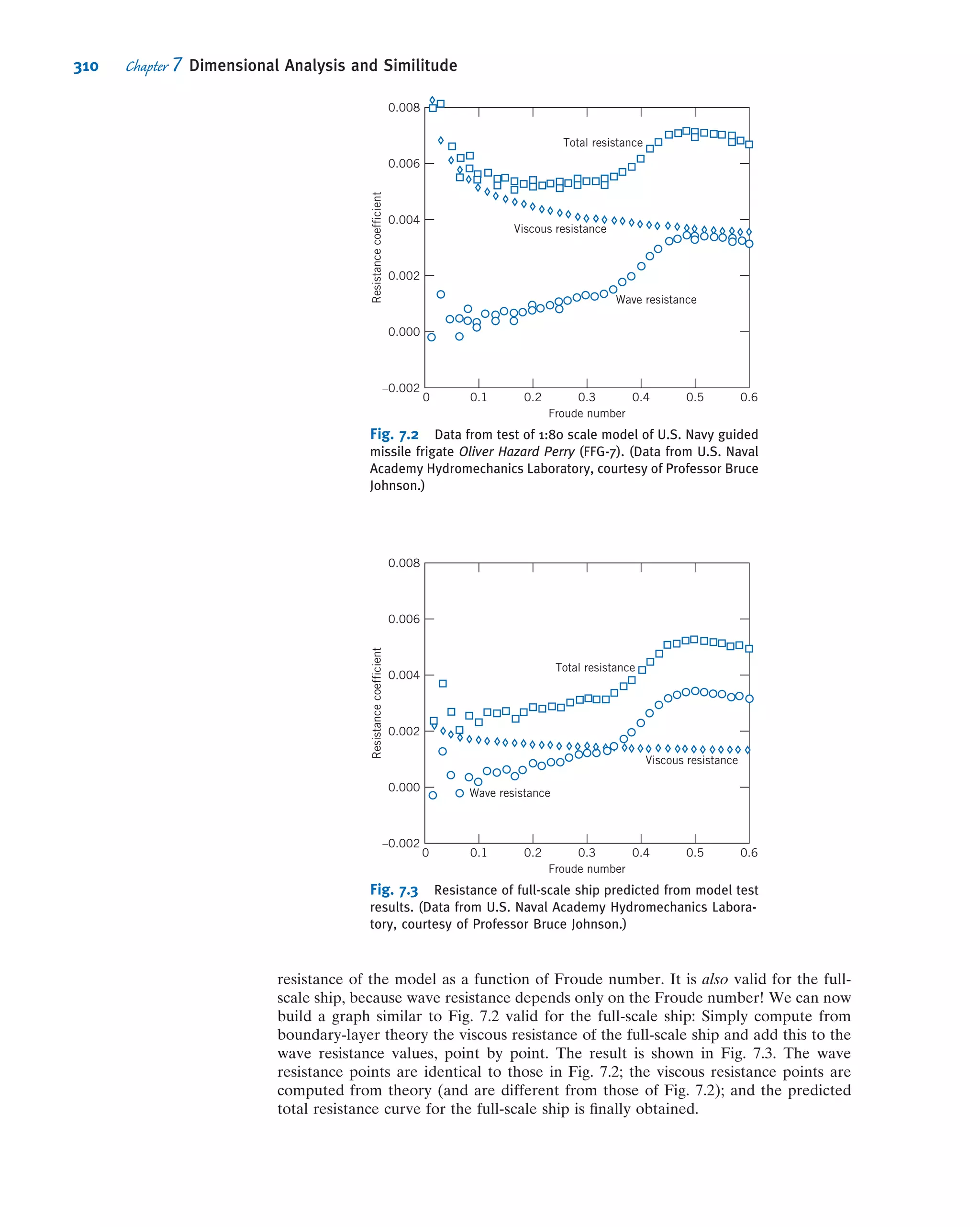

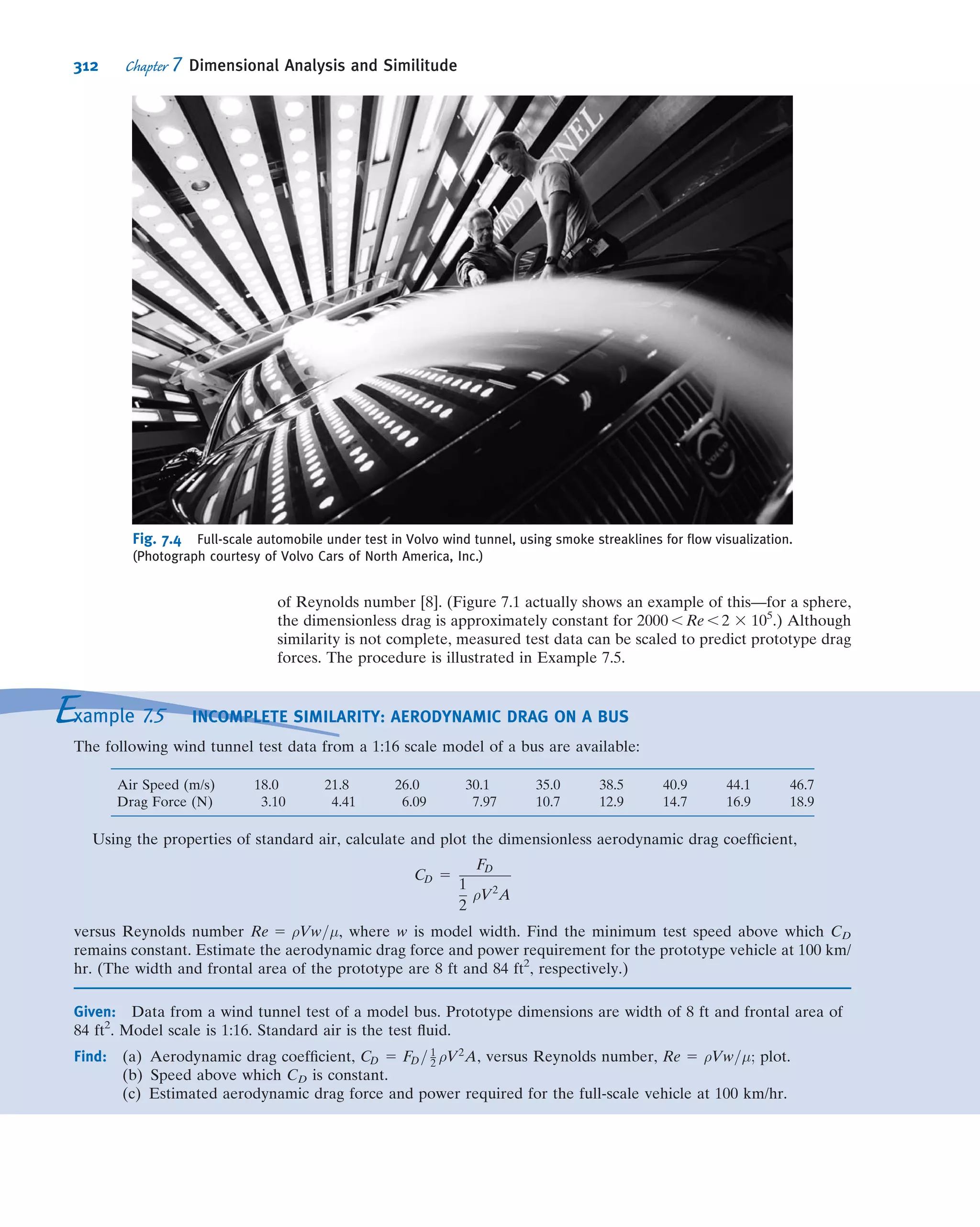


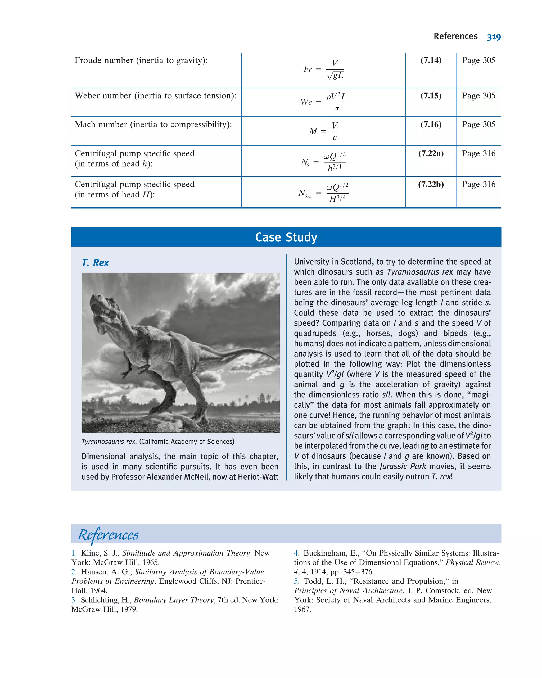
![u*
@u*
@x*
1 v*
@u*
@y*
5 2
@p*
@x*
1
μ
ρVNL
@2
u*
@x*2
1
@2
u*
@y*2
ð7:9Þ
u*
@v*
@x*
1 v*
@v*
@y*
5 2
gL
V2
N
2
@p*
@y*
1
μ
ρVNL
@2
v*
@x*2
1
@2
v*
@y*2
ð7:10Þ
Equations 7.8, 7.9, and 7.10 are the nondimensional forms of our original equations
(Eqs. 7.1, 7.2, 7.3). As such, we can think about their solution (with appropriate
boundary conditions) as an exercise in applied mathematics. Equation 7.9 contains a
dimensionless coefficient μ/ρVNL (which we recognize as the inverse of the Reynolds
number) in front of the second-order (viscous) terms; Eq. 7.10 contains this and
another dimensionless coefficient, gL/V2
N (which we will discuss shortly) for the
gravity force term. We recall from the theory of differential equations that
the mathematical form of the solution of such equations is very sensitive to the values
of the coefficients in the equations (e.g., certain second-order partial differential
equations can be elliptical, parabolic, or hyperbolic depending on coefficient values).
These equations tell us that the solution, and hence the actual flow pattern they
describe, depends on the values of the two coefficients. For example, if μ/ρVNL is
very small (i.e., we have a high Reynolds number), the second-order differentials,
representing viscous forces, can be neglected, at least in most of the flow, and we end
up with a form of Euler’s equations (Eqs. 6.2). We say “in most of the flow” because
we have already learned that in reality for this case we will have a boundary layer in
which there is significant effect of viscosity; in addition, from a mathematical point of
view, it is always dangerous to neglect higher-order derivatives, even if their coeffi-
cients are small, because reduction to a lower-order equation means we lose a
boundary condition (specifically the no-slip condition). We can predict that if μ/ρVNL
is large or small, then viscous forces will be significant or not, respectively; if gLV2
N is
large or small, we can predict that gravity forces will be significant or not, respectively.
We can thus gain insight even before attempting a solution to the differential equa-
tions. Note that for completeness, we would have to apply the same non-
dimensionalizing approach to the boundary conditions of the problem, which often
introduce further dimensionless coefficients.
Writing nondimensional forms of the governing equations, then, can yield insight
into the underlying physical phenomena, and indicate which forces are dominant. If
we had two geometrically similar but different scale flows satisfying Eqs. 7.8, 7.9, and
7.10 (for example, a model and a prototype), the equations would only yield the same
mathematical results if the two flows had the same values for the two coefficients (i.e.,
had the same relative importance of gravity, viscous, and inertia forces). This non-
dimensional form of the equations is also the starting point in numerical methods,
which is very often the only way of obtaining their solution. Additional derivations
and examples of establishing similitude from the governing equations of a problem
are presented in Kline [1] and Hansen [2].
We will now see how the method of dimensional analysis can be used instead of the
above procedure to find appropriate dimensionless groupings of physical parameters.
As we have mentioned, using dimensionless groupings is very useful for experimental
measurements, and we will see in the next two sections that we can obtain them even
when we do not have the governing equations such as Eqs. 7.1, 7.2, and 7.3 to work from.
7.2 Nature of Dimensional Analysis
Most phenomena in fluid mechanics depend in a complex way on geometric and flow
parameters. For example, consider the drag force on a stationary smooth sphere
immersed in a uniform stream. What experiments must be conducted to determine the
294 Chapter 7 Dimensional Analysis and Similitude](https://image.slidesharecdn.com/foxphilipj-160402150646/75/Fox-Philip-J-Pritchard-8-ed-Mc-Donald-s-Introduction-to-Fluid-Mechanics-wiley-2011-342-2048.jpg)

![sphere) as it moves through the aorta—in either case, given the fluid (ρ and μ), the
flow speed V, and the sphere diameter D, we could compute a value for ρVD/μ, then
read the corresponding value for CD, and finally compute the drag force F.
In Section 7.3 we introduce the Buckingham Pi theorem, a formalized procedure
for deducing the dimensionless groups appropriate for a given fluid mechanics or
other engineering problem. This section, and Section 7.4, may seem a bit difficult to
follow; we suggest you read them once, then study Examples 7.1, 7.2, and 7.3 to see
how practical and useful the method in fact is, before returning to the two sections for
a reread.
The Buckingham Pi theorem is a statement of the relation between a function
expressed in terms of dimensional parameters and a related function expressed in
terms of nondimensional parameters. The Buckingham Pi theorem allows us to
develop the important nondimensional parameters quickly and easily.
7.3 Buckingham Pi Theorem
In the previous section we discussed how the drag F on a sphere depends on the
sphere diameter D, fluid density ρ and viscosity μ, and fluid speed V, or
F 5 FðD, ρ, μ, VÞ
with theory or experiment being needed to determine the nature of function f. More
formally, we write
gðF, D, ρ, μ, VÞ 5 0
where g is an unspecified function, different from f. The Buckingham Pi theorem [4]
states that we can transform a relationship between n parameters of the form
gðq1, q2, . . . , qnÞ 5 0
into a corresponding relationship between n 2 m independent dimensionless Π
parameters in the form
GðΠ1, Π2, . . . , Πn2mÞ 5 0
400
200
100
60
40
20
10
6
4
2
1
0.6
0.4
0.2
0.1
0.06
10–1
100
101
1022 224 446 688 8 2 4 68103 2 4 68104 2 4 68105
1062 4 686
VD____ρ
μ
F___________
V21__
2
ρ π D2
___
4
Fig. 7.1 Experimentally derived relation between the nondimensional parameters [3].
296 Chapter 7 Dimensional Analysis and Similitude](https://image.slidesharecdn.com/foxphilipj-160402150646/75/Fox-Philip-J-Pritchard-8-ed-Mc-Donald-s-Introduction-to-Fluid-Mechanics-wiley-2011-344-2048.jpg)

![Similarly,
Π2 5 ρd
Ve
Df
μ and
M
L3
d
L
t
e
ðLÞf M
Lt
5 M0
L0
t0
M : d 1 1 5 0 d 5 21
L : 23d 1 e 1 f 2 1 5 0 f 5 21
t : 2e 2 1 5 0 e 5 21
9
=
;
Therefore, Π2 5
μ
ρVD
6 Check using F, L, t dimensions
½Π1Š 5
F
ρV2D2
and F
L4
Ft2
t
L
2 1
L2
5 1
where [ ] means “has dimensions of,” and
½Π2Š 5
μ
ρVD
and
Ft
L2
L4
Ft2
t
L
1
L
5 1
The functional relationship is Π1 5 f(Π2), or
F
ρV2D2
5 f
μ
ρVD
as noted before. The form of the function, f, must be determined
experimentally (see Fig. 7.1).
The Excel workbook for thisExample is convenient for com-
puting the values of a, b, and c for this
and other problems.
Example 7.2 PRESSURE DROP IN PIPE FLOW
The pressure drop, Δp, for steady, incompressible viscous flow through a straight horizontal pipe depends on the
pipe length, l, the average velocity, V, the fluid viscosity, μ, the pipe diameter, D, the fluid density, ρ, and the average
“roughness” height, e. Determine a set of dimensionless groups that can be used to correlate data.
Given: Δp 5 f(ρ, V, D, l, μ, e) for flow in a circular pipe.
Find: A suitable set of dimensionless groups.
Solution:
(Circled numbers refer to steps in the procedure for determining dimensionless Π parameters.)
1 Δp ρ μ V l D e n 5 7 dimensional parameters
2 Choose primary dimensions M, L, and t.
3 Δp ρ μ V l D e
M
Lt2
M
L3
M
Lt
L
t
L L L r 5 3 primary dimensions
4 Select repeating parameters ρ, V, D. m 5 r 5 3 repeating parameters
7.4 Determining the Π Groups 299](https://image.slidesharecdn.com/foxphilipj-160402150646/75/Fox-Philip-J-Pritchard-8-ed-Mc-Donald-s-Introduction-to-Fluid-Mechanics-wiley-2011-347-2048.jpg)


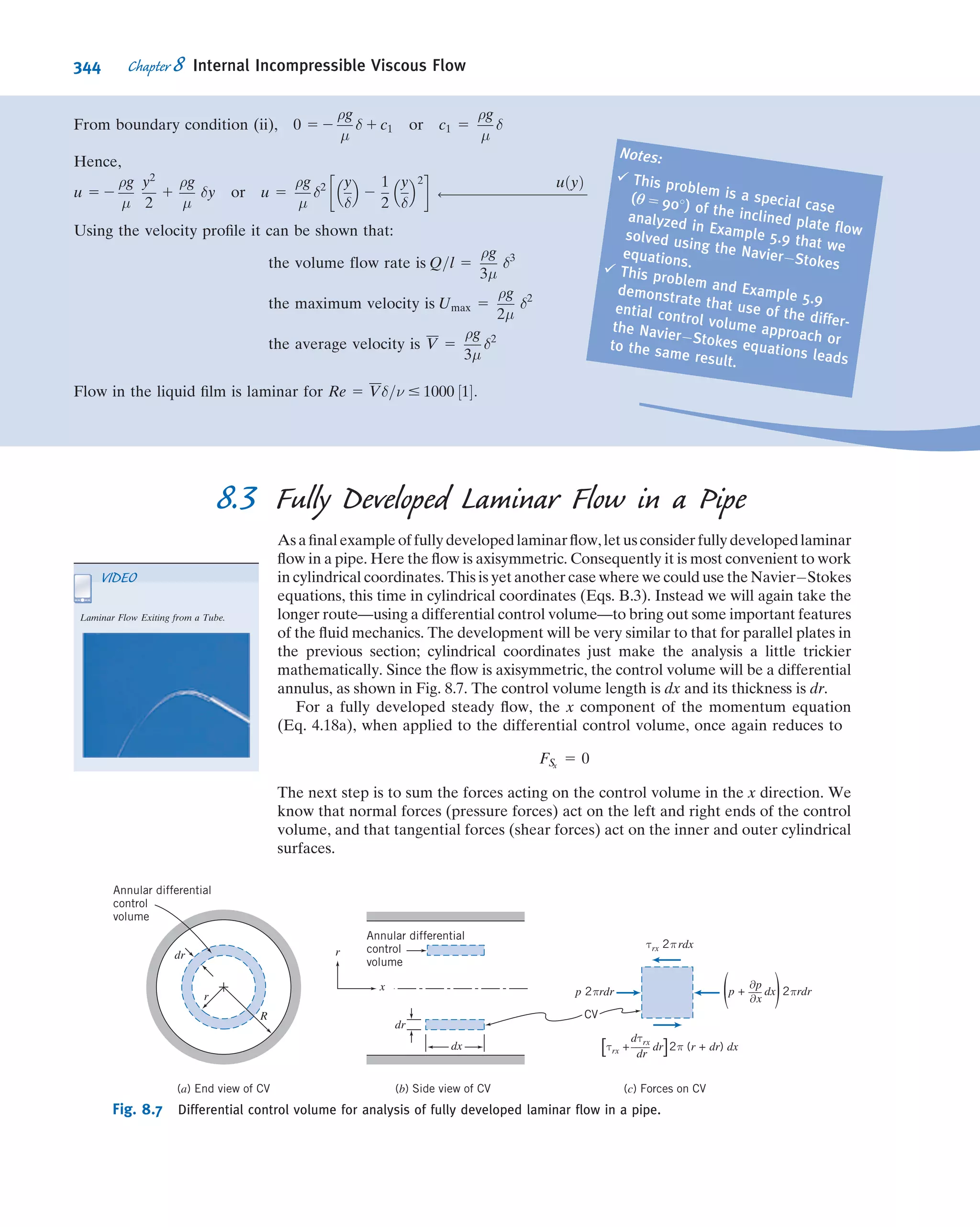

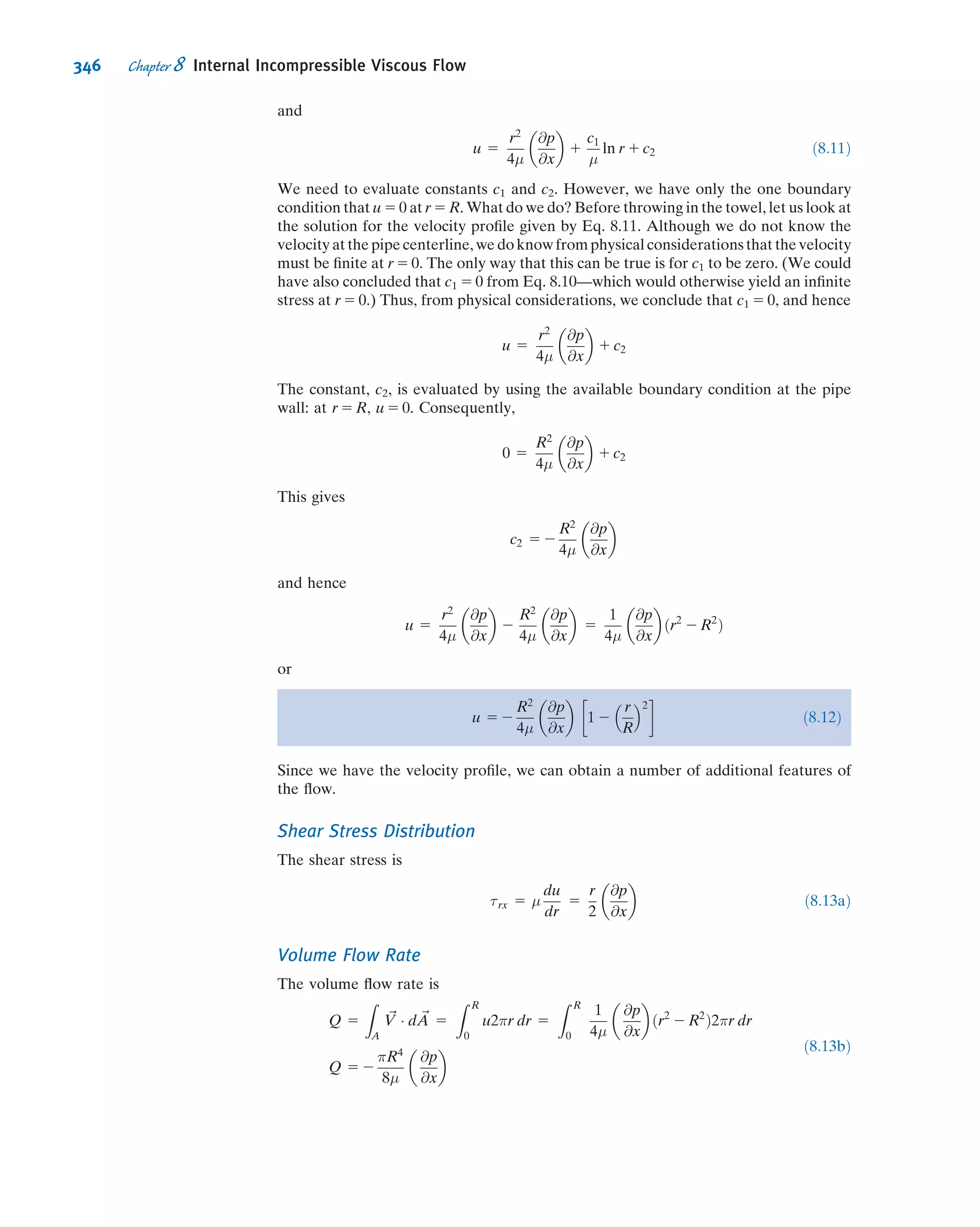

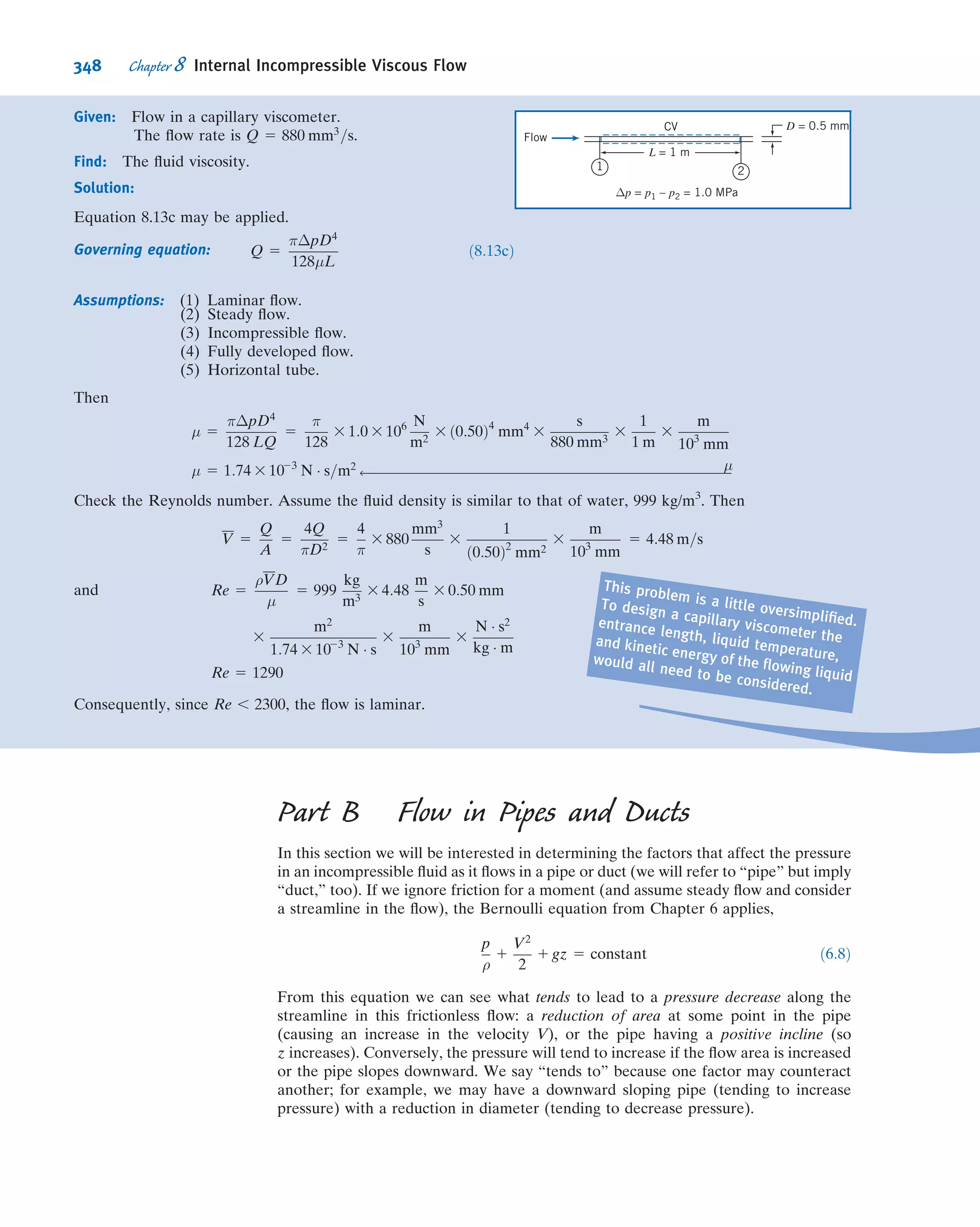

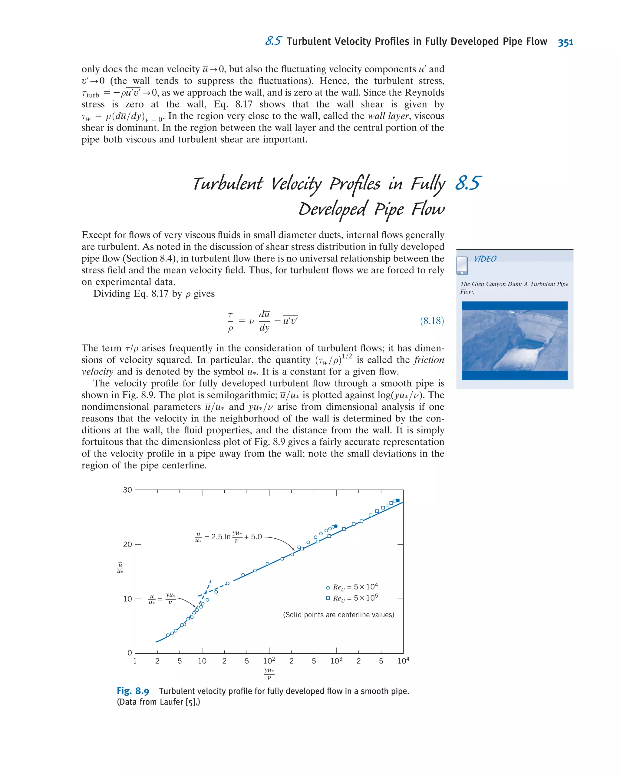


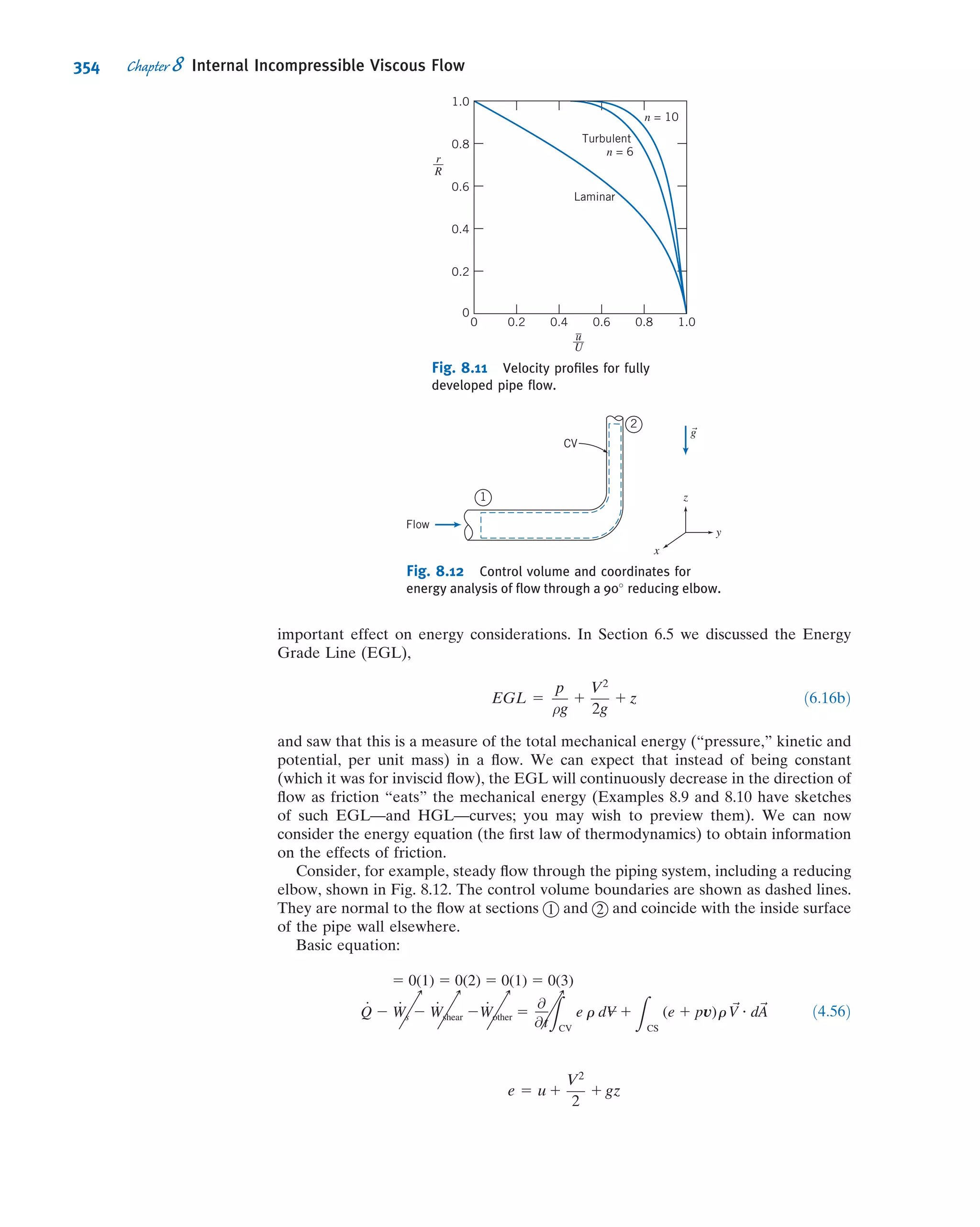


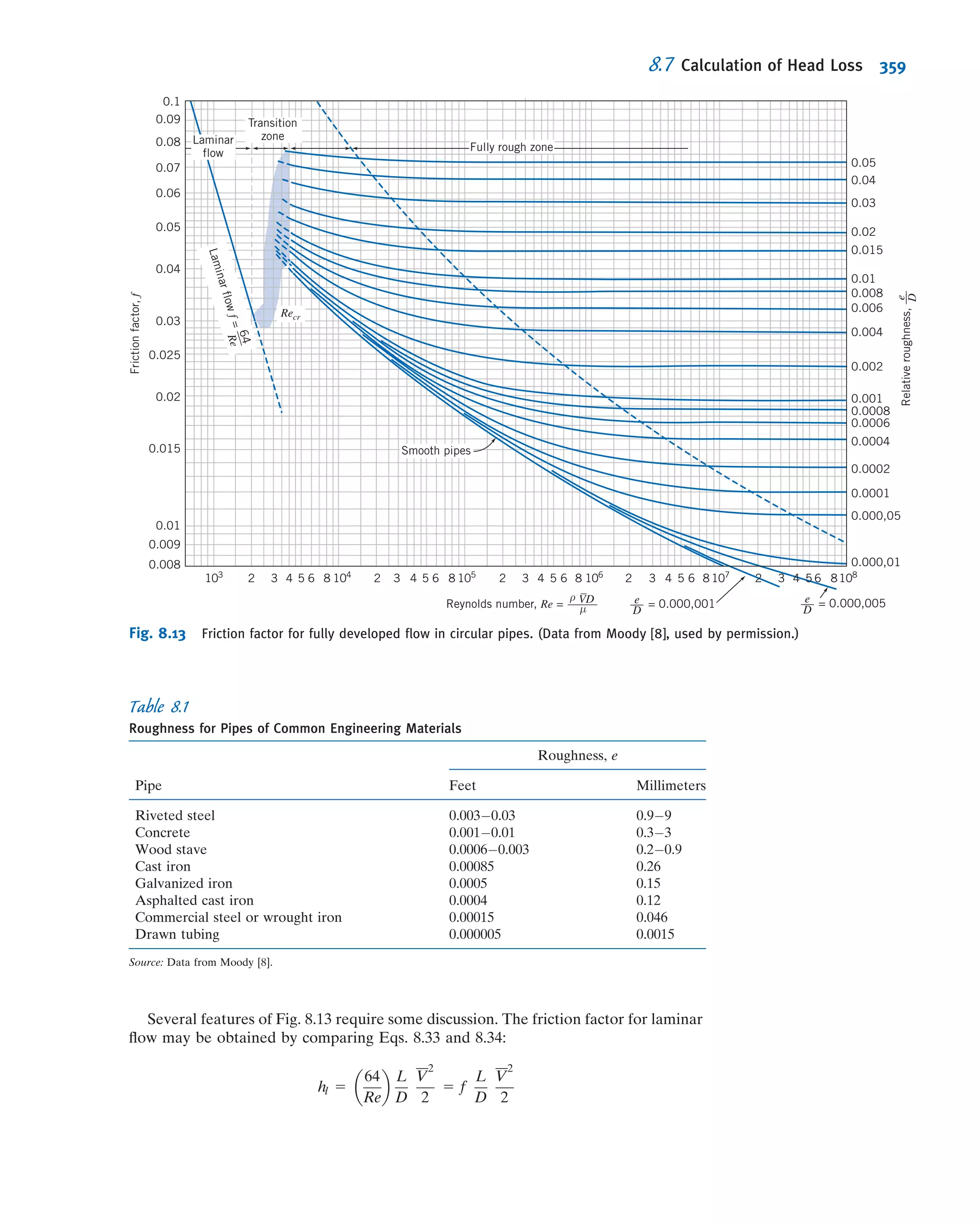
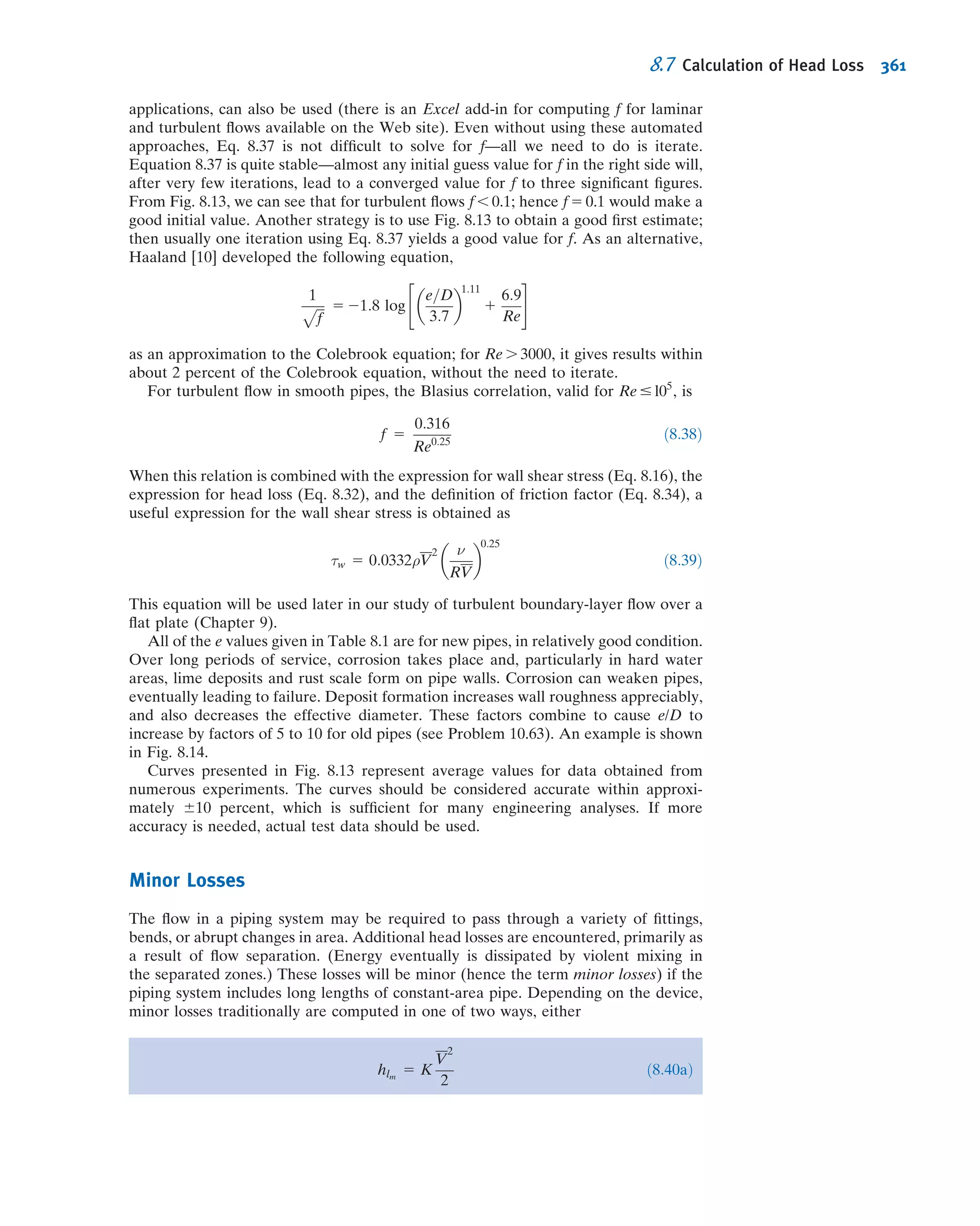


![In this example, incomplete modeling was overcome by using analytical compu-
tations; the model experiments modeled the Froude number, but not the Reynolds
number.
Because the Reynolds number cannot be matched for model tests of surface ships,
the boundary-layer behavior is not the same for model and prototype. The model
Reynolds number is only (Lm/Lp)3/2
as large as the prototype value, so the extent of
laminar flow in the boundary layer on the model is too large by a corresponding
factor. The method just described assumes that boundary-layer behavior can be
scaled. To make this possible, the model boundary layer is “tripped” or “stimulated”
to become turbulent at a location that corresponds to the behavior on the full-scale
vessel. “Studs” were used to stimulate the boundary layer for the model test results
shown in Fig. 7.2.
A correction sometimes is added to the full-scale coefficients calculated from
model test data. This correction accounts for roughness, waviness, and unevenness
that inevitably are more pronounced on the full-scale ship than on the model. Com-
parisons between predictions from model tests and measurements made in full-scale
trials suggest an overall accuracy within 65 percent [5].
As we will see in Chapter 11, the Froude number is an important parameter in the
modeling of rivers and harbors. In these situations it is not practical to obtain com-
plete similarity. Use of a reasonable model scale would lead to extremely small water
depths, so that viscous forces and surface tension forces would have much larger
relative effects in the model flow than in the prototype. Consequently, different length
scales are used for the vertical and horizontal directions. Viscous forces in the deeper
model flow are increased using artificial roughness elements.
Emphasis on fuel economy has made reduction of aerodynamic drag important for
automobiles, trucks, and buses. Most work on development of low-drag configurations
is done using model tests. Traditionally, automobile models have been built to 3
8 scale,
at which a model of a full-size automobile has a frontal area of about 0.3 m2
. Thus
testing can be done in a wind tunnel with test section area of 6 m2
or larger. At 3
8 scale,
a wind speed of about 150 mph is needed to model a prototype automobile traveling
at the legal speed limit. Thus there is no problem with compressibility effects, but the
scale models are expensive and time-consuming to build.
A large wind tunnel (test section dimensions are 5.4 m high, 10.4 m wide, and
21.3 m long; maximum air speed is 250 km/hr with the tunnel empty) is used by
General Motors to test full-scale automobiles at highway speeds. The large test sec-
tion allows use of production autos or of full-scale clay mockups of proposed auto
body styles. Many other vehicle manufacturers are using comparable facilities; Fig. 7.4
shows a full-size sedan under test in the Volvo wind tunnel. The relatively low speed
permits flow visualization using tufts or “smoke” streams.1
Using full-size “models,”
stylists and engineers can work together to achieve optimum results.
It is harder to achieve dynamic similarity in tests of trucks and buses; models must
be made to smaller scale than those for automobiles.2
A large scale for truck and bus
testing is 1:8. To achieve complete dynamic similarity by matching Reynolds numbers
at this scale would require a test speed of 440 mph. This would introduce unwanted
compressibility effects, and model and prototype flows would not be kinematically
similar. Fortunately, trucks and buses are “bluff” objects. Experiments show that
above a certain Reynolds number, their nondimensional drag becomes independent
1
A mixture of liquid nitrogen and steam may be used to produce “smoke” streaklines that evaporate and do
not clog the fine mesh screens used to reduce the turbulence level in a wind tunnel. Streaklines may be made
to appear “colored” in photos by placing a filter over the camera lens. This and other techniques for flow
visualization are detailed in Reference [6] and Merzkirch [7].
2
The vehicle length is particularly important in tests at large yaw angles to simulate crosswind behavior.
Tunnel blockage considerations limit the acceptable model size. See Reference [8] for recommended
practices.
7.6 Flow Similarity and Model Studies 311](https://image.slidesharecdn.com/foxphilipj-160402150646/75/Fox-Philip-J-Pritchard-8-ed-Mc-Donald-s-Introduction-to-Fluid-Mechanics-wiley-2011-387-2048.jpg)
![of Reynolds number [8]. (Figure 7.1 actually shows an example of this—for a sphere,
the dimensionless drag is approximately constant for 2000 , Re , 2 3 105
.) Although
similarity is not complete, measured test data can be scaled to predict prototype drag
forces. The procedure is illustrated in Example 7.5.
Fig. 7.4 Full-scale automobile under test in Volvo wind tunnel, using smoke streaklines for flow visualization.
(Photograph courtesy of Volvo Cars of North America, Inc.)
Example 7.5 INCOMPLETE SIMILARITY: AERODYNAMIC DRAG ON A BUS
The following wind tunnel test data from a 1:16 scale model of a bus are available:
Air Speed (m/s) 18.0 21.8 26.0 30.1 35.0 38.5 40.9 44.1 46.7
Drag Force (N) 3.10 4.41 6.09 7.97 10.7 12.9 14.7 16.9 18.9
Using the properties of standard air, calculate and plot the dimensionless aerodynamic drag coefficient,
CD 5
FD
1
2
ρV2
A
versus Reynolds number Re 5 ρVw=μ, where w is model width. Find the minimum test speed above which CD
remains constant. Estimate the aerodynamic drag force and power requirement for the prototype vehicle at 100 km/
hr. (The width and frontal area of the prototype are 8 ft and 84 ft2
, respectively.)
Given: Data from a wind tunnel test of a model bus. Prototype dimensions are width of 8 ft and frontal area of
84 ft2
. Model scale is 1:16. Standard air is the test fluid.
Find: (a) Aerodynamic drag coefficient, CD 5 FD= 1
2 ρV2
A, versus Reynolds number, Re 5 ρVw=μ; plot.
(b) Speed above which CD is constant.
(c) Estimated aerodynamic drag force and power required for the full-scale vehicle at 100 km/hr.
312 Chapter 7 Dimensional Analysis and Similitude](https://image.slidesharecdn.com/foxphilipj-160402150646/75/Fox-Philip-J-Pritchard-8-ed-Mc-Donald-s-Introduction-to-Fluid-Mechanics-wiley-2011-388-2048.jpg)

![For additional details on techniques and applications of dimensional analysis
consult [9À12].
Scaling with Multiple Dependent Parameters
In some situations of practical importance there may be more than one dependent
parameter. In such cases, dimensionless groups must be formed separately for each
dependent parameter.
As an example, consider a typical centrifugal pump. The detailed flow pattern
within a pump changes with volume flow rate and speed; these changes affect the
pump’s performance. Performance parameters of interest include the pressure rise (or
head) developed, the power input required, and the machine efficiency measured
under specific operating conditions.3
Performance curves are generated by varying an
independent parameter such as the volume flow rate. Thus the independent variables
are volume flow rate, angular speed, impeller diameter, and fluid properties.
Dependent variables are the several performance quantities of interest.
Finding dimensionless parameters begins from the symbolic equations for the
dependence of head, h (energy per unit mass, L2
/t2
), and power, 3, on the indepen-
dent parameters, given by
h 5 g1ðQ, ρ, ω, D, μÞ
and
3 5 g2ðQ, ρ, ω, D, μÞ
Straightforward use of the Pi theorem gives the dimensionless head coefficient and
power coefficient as
h
ω2D2
5 f1
Q
ωD3
,
ρωD2
μ
ð7:17Þ
The corresponding power required to overcome aerodynamic drag is
3p 5 FDp
Vp
5 1:71 3 103
N 3 100
km
hr
3 1000
m
km
3
hr
3600 s
3
W Ás
N Á m
3p 5 47:5 kW ß
3p
This problem illustrates a common
phenomenon in aerodynamics: Above a
certain minimum Reynolds number the
drag coefficient of an object usually
approaches a constant—that is,
becomes independent of the Reynolds
number. Hence, in these situations we
do not have to match the Reynolds
numbers of the model and prototype in
order for them to have the same drag
coefficient—a considerable advantage.
However, the SAE Recommended
Practices [8] suggests Re $ 2 3 106
for
truck and bus testing.
3
Efficiency is defined as the ratio of power delivered to the fluid divided by input power, η 5 3/3in. For
incompressible flow, we will see in Chapter 8 that the energy equation reduces to 3 5 ρQh (when “head” h
is expressed as energy per unit mass) or to 3 5 ρgQH (when head H is expressed as energy per unit weight).
314 Chapter 7 Dimensional Analysis and Similitude](https://image.slidesharecdn.com/foxphilipj-160402150646/75/Fox-Philip-J-Pritchard-8-ed-Mc-Donald-s-Introduction-to-Fluid-Mechanics-wiley-2011-390-2048.jpg)

![Comments on Model Testing
While outlining the procedures involved in model testing, we have tried not to imply
that testing is a simple task that automatically gives results that are easily interpreted,
accurate, and complete. As in all experimental work, careful planning and execution
are needed to obtain valid results. Models must be constructed carefully and accu-
rately, and they must include sufficient detail in areas critical to the phenomenon
being measured. Aerodynamic balances or other force measuring systems must be
aligned carefully and calibrated correctly. Mounting methods must be devised that
offer adequate rigidity and model motion, yet do not interfere with the phenomenon
being measured. References [13À15] are considered the standard sources for details
of wind tunnel test techniques. More specialized techniques for water impact testing
are described in Waugh and Stubstad [16].
Experimental facilities must be designed and constructed carefully. The quality
of flow in a wind tunnel must be documented. Flow in the test section should be
as nearly uniform as possible (unless the desire is to simulate a special profile
such as an atmospheric boundary layer), free from angularity, and with little swirl. If
they interfere with measurements, boundary layers on tunnel walls must be
removed by suction or energized by blowing. Pressure gradients in a wind tunnel
test section may cause erroneous drag-force readings due to pressure variations in
the flow direction.
Special facilities are needed for unusual conditions or for special test requirements,
especially to achieve large Reynolds numbers. Many facilities are so large or spe-
cialized that they cannot be supported by university laboratories or private industry.
A few examples include [17À19]:
Then H/ω2
D2
5 constant, so
H2 5 H1
ω2
ω1
2
D2
D1
2
5 21:9 ft
1750
1170
2
ð1Þ2
5 49:0 ft ß
H2
The pump output power is 31 5 ρgQ1H1, so at ω1 5 1170 rpm,
31 5 1:94
slug
ft3
3 32:2
ft
s2
3 300
gal
min
3 21:9 ft 3
ft3
7:48 gal
3
min
60 s
3
lbf Á s2
slug Á ft
3
hp Á s
550 ft Á lbf
31 5 1:66 hp
But 3=ρω3
D5
5 constant, so
32 5 31
ρ2
ρ1
ω2
ω1
3
D2
D1
5
5 1:66 hpð1Þ
1750
1170
3
ð1Þ5
5 5:55 hp ß
32
The required input power may be calculated as
3in 5
32
η
5
5:55 hp
0:80
5 6:94 hp ß
3in
Thus a 7.5-hp motor (the next larger standard size) probably would be
specified.
The specific speed at ω2 5 1750 rpm is
Nscu
5
ωQ1=2
H3=4
5
1750ð449Þ1=2
ð49:0Þ3=4
5 2000 ß
Nscu
This problem illustrates application of
the pump “laws” and specific speed to
scaling of performance data. Pump and
fan “laws” are used widely in industry
to scale performance curves for fam-
ilies of machines from a single perfor-
mance curve, and to specify drive
speed and power in machineapplications.
7.6 Flow Similarity and Model Studies 317](https://image.slidesharecdn.com/foxphilipj-160402150646/75/Fox-Philip-J-Pritchard-8-ed-Mc-Donald-s-Introduction-to-Fluid-Mechanics-wiley-2011-393-2048.jpg)
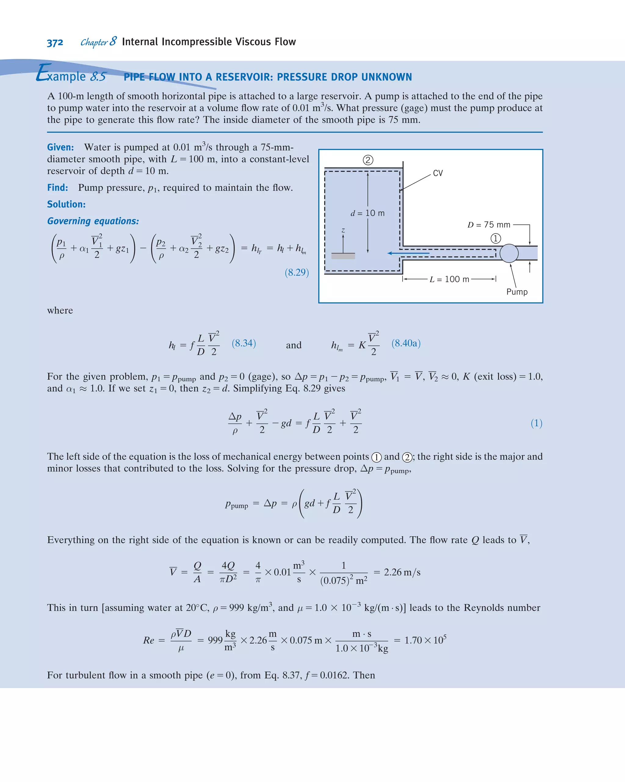


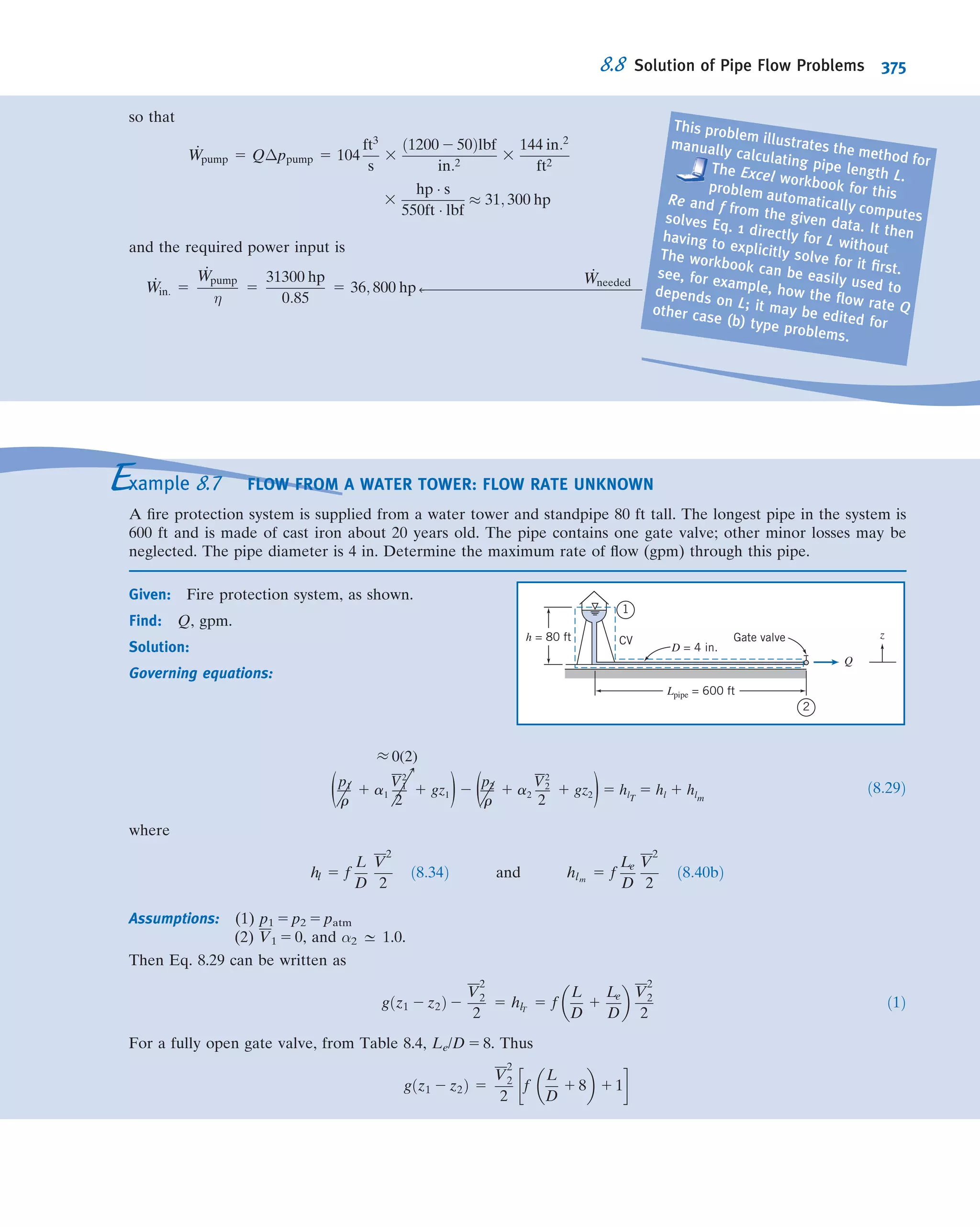
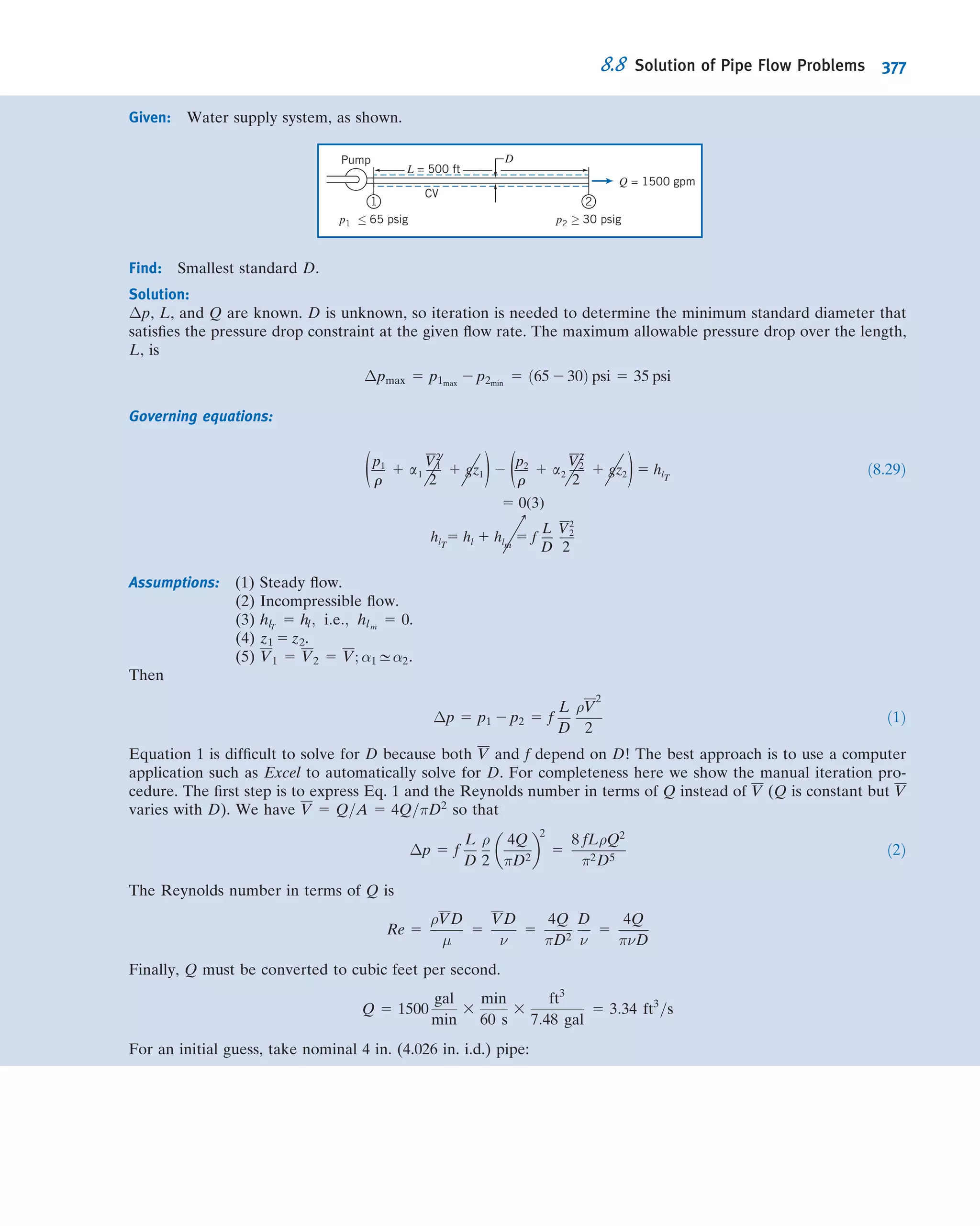

![the air temperature. Calculate the equivalent speed for the
wind tunnel using air at 40
F and 150
F. Would replacing air
with carbon dioxide provide higher equivalent speeds?
7.80 Consider water flow around a circular cylinder, of diam-
eter D and length l. In addition to geometry, the drag force
is known to depend on liquid speed, V, density, ρ, and vis-
cosity, μ. Express drag force, FD, in dimensionless form as a
function of all relevant variables. The static pressure dis-
tribution on a circular cylinder, measured in the laboratory,
can be expressed in terms of the dimensionless pressure
coefficient; the lowest pressure coefficient is Cp 5 22.4
at the location of the minimum static pressure on the
cylinder surface. Estimate the maximum speed at which
a cylinder could be towed in water at atmospheric pressure,
without causing cavitation, if the onset of cavitation occurs at
a cavitation number of 0.5.
7.81 A circular container, partially filled with water, is
rotated about its axis at constant angular speed, ω. At any
time, τ, from the start of rotation, the speed, Vθ, at distance r
from the axis of rotation, was found to be a function of τ, ω,
and the properties of the liquid. Write the dimensionless
parameters that characterize this problem. If, in another
experiment, honey is rotated in the same cylinder at the
same angular speed, determine from your dimensionless
parameters whether honey will attain steady motion as
quickly as water. Explain why the Reynolds number would
not be an important dimensionless parameter in scaling the
steady-state motion of liquid in the container.
7.82 A 1
10-scale model of a tractor-trailer rig is tested in a
wind tunnel. The model frontal area is Am 5 0.1 m2
. When
tested at Vm 5 75 m/s in standard air, the measured drag
force is FD 5 350 N. Evaluate the drag coefficient for the
model conditions given. Assuming that the drag coefficient is
the same for model and prototype, calculate the drag force
on a prototype rig at a highway speed of 90 km/hr. Deter-
mine the air speed at which a model should be tested to
ensure dynamically similar results if the prototype speed is
90 km/hr. Is this air speed practical? Why or why not?
7.83 It is recommended in [8] that the frontal area of a model
be less than 5 percent of the wind tunnel test section area and
Re 5 Vw/ν . 2 3 106
, where w is the model width. Further,
the model height must be less than 30 percent of the test
section height, and the maximum projected width of the
model at maximum yaw (20
) must be less than 30 percent
of the test section width. The maximum air speed should be
less than 300 ft/s to avoid compressibility effects. A model of
a tractor-trailer rig is to be tested in a wind tunnel that has a
test section 1.5 ft high and 2 ft wide. The height, width, and
length of the full-scale rig are 13 ft 6 in., 8 ft, and 65 ft,
respectively. Evaluate the scale ratio of the largest model
that meets the recommended criteria. Assess whether an
adequate Reynolds number can be achieved in this test
facility.
7.84 The power, 3, required to drive a fan is assumed
to depend on fluid density ρ, volume flow rate Q, impeller
diameter D, and angular speed ω. If a fan with D1 = 8 in.
delivers Q1 = 15 ft3
/s of air at ω1 = 2500 rpm, what
size diameter fan could be expected to deliver Q2 = 88 ft3
/s of
air at ω2 = 1800 rpm, provided they were geometrically and
dynamically similar?
7.85 Over a certain range of air speeds, V, the lift, FL, pro-
duced by a model of a complete aircraft in a wind tunnel
depends on the air speed, air density, ρ, and a characteristic
length (the wing base chord length, c 5 150 mm). The fol-
lowing experimental data is obtained for air at standard
atmospheric conditions:
V (m/s) 10 15 20 25 30 35 40 45 50
FL (N) 2.2 4.8 8.7 13.3 19.6 26.5 34.5 43.8 54
Plot the lift versus speed curve. By using Excel to perform a
trendline analysis on this curve, generate and plot data for
the lift produced by the prototype, which has a wing base
chord length of 5 m, over a speed range of 75 m/s to 250 m/s.
7.86 The pressure rise, Δp, of a liquid flowing steadily
through a centrifugal pump depends on pump diameter D,
angular speed of the rotor ω, volume flow rate Q, and density
ρ. The table gives data for the prototype and for a geomet-
rically similar model pump. For conditions corresponding to
dynamic similarity between the model and prototype pumps,
calculate the missing values in the table.
Variable Prototype Model
Δp 52.5 kPa
Q 0.0928 m3
/min
ρ 800 kg/m3
999 kg/m3
ω 183 rad/s 367 rad/s
D 150 mm 50 mm
7.87 Tests are performed on a 3-ft-long ship model in a water
tank. Results obtained (after doing some data analysis) are
as follows:
V (ft/s) 10 20 30 40 50 60 70
DWave (lbf) 0 0.028 0.112 0.337 0.674 0.899 1.237
DFriction (lbf) 0.022 0.079 0.169 0.281 0.45 0.618 0.731
The assumption is that wave drag is done using the Froude
number and friction drag by the Reynolds number. The full-
size ship will be 150 ft long when built. Estimate the total
drag when it is cruising at 15 knots and at 20 knots in a
freshwater lake.
7.88 A centrifugal water pump running at speed ω = 800 rpm
has the following data for flow rate, Q, and pressure head, Δp.
Q (ft3
/min) 0 50 75 100 120 140 150 165
Δp (psf) 7.54 7.29 6.85 6.12 4.80 3.03 2.38 1.23
The pressure head is a function of the flow rate, speed,
impeller diameter D, and water density ρ. Plot the pressure
head versus flow rate curve. Find the two Π parameters for
this problem, and, from the above data, plot one against the
other. By using Excel to perform a trendline analysis on this
latter curve, generate and plot data for pressure head versus
flow rate for impeller speeds of 600 rpm and 1200 rpm.
7.89 An axial-flow pump is required to deliver 0.75 m3
/s of
water at a head of 15 J/kg. The diameter of the rotor is 0.25 m,
and it is to be driven at 500 rpm. The prototype is to be modeled
326 Chapter 7 Dimensional Analysis and Similitude](https://image.slidesharecdn.com/foxphilipj-160402150646/75/Fox-Philip-J-Pritchard-8-ed-Mc-Donald-s-Introduction-to-Fluid-Mechanics-wiley-2011-402-2048.jpg)


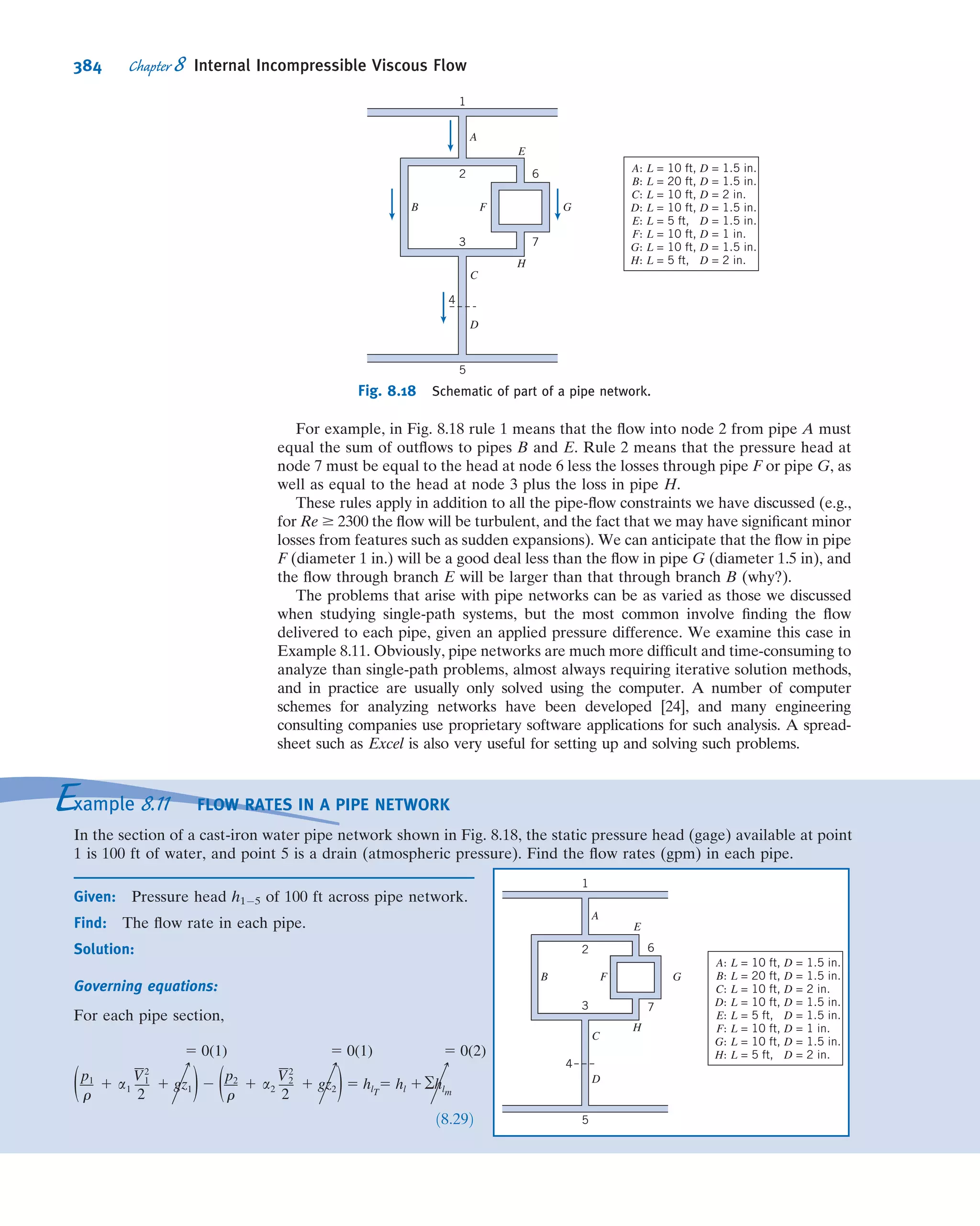


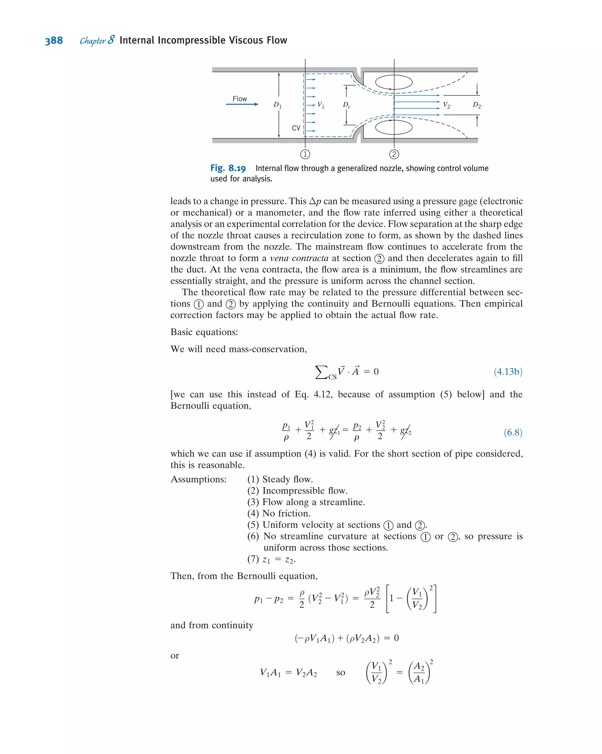
![it does not change with x). Hence, the only way the equation can be valid for all x and
y is for each side to in fact be constant:
dτyx
dy
5
@p
@x
5 constant
Integrating this equation, we obtain
τyx 5
@p
@x
y 1 c1
which indicates that the shear stress varies linearly with y. We wish to find the velocity
distribution. To do so, we need to relate the shear stress to the velocity field. For a
Newtonian fluid we can use Eq. 2.15 because we have a one-dimensional flow [or we
could have started with the full stress equation (Eq. 5.25a) and simplified],
τyx 5 μ
du
dy
ð2:15Þ
so we get
μ
du
dy
5
@p
@x
y 1 c1
Integrating again
u 5
1
2μ
@p
@x
y2
1
c1
μ
y 1 c2 ð8:4Þ
It is interesting to note that if we had started with the NavierÀStokes equations
(Eqs. 5.27) instead of using a differential control volume, after only a few steps (i.e.,
simplifying and integrating twice) we would have obtained Eq. 8.4 (see Problem 8.17).
To evaluate the constants, c1 and c2, we must apply the boundary conditions. At y 5 0,
u 5 0. Consequently, c2 5 0. At y 5 a, u 5 0. Hence
0 5
1
2μ
@p
@x
a2
1
c1
μ
a
This gives
c1 5 2
1
2
@p
@x
a
and hence,
u 5
1
2μ
@p
@x
y2
2
1
2μ
@p
@x
ay 5
a2
2μ
@p
@x
y
a
2
2
y
a
ð8:5Þ
At this point we have the velocity profile. This is key to finding other flow properties,
as we next discuss.
Shear Stress Distribution
The shear stress distribution is given by
τyx 5
@p
@x
y 1 c1 5
@p
@x
y 2
1
2
@p
@x
a 5 a
@p
@x
y
a
2
1
2
ð8:6aÞ
8.2 Fully Developed Laminar Flow Between Infinite Parallel Plates 335](https://image.slidesharecdn.com/foxphilipj-160402150646/75/Fox-Philip-J-Pritchard-8-ed-Mc-Donald-s-Introduction-to-Fluid-Mechanics-wiley-2011-411-2048.jpg)


![Since only the boundary conditions have changed, there is no need to repeat the entire
analysis of the previous section. The analysis leading to Eq. 8.4 is equally valid for the
moving plate case. Thus the velocity distribution is given by
u 5
1
2μ
@p
@x
y2
1
c1
μ
y 1 c2 ð8:4Þ
and our only task is to evaluate constants c1 and c2 by using the appropriate boundary
conditions. [Note once again that using the full NavierÀStokes equations (Eqs. 5.27)
would have led very quickly to Eq. 8.4.]
At y 5 0; u 5 0: Consequently; c2 5 0:
At y 5 a; u 5 U: Consequently;
U 5
1
2μ
@p
@x
a2
1
c1
μ
a and thus c1 5
Uμ
a
2
1
2
@p
@x
a
Hence,
u 5
1
2μ
@p
@x
y2
1
Uy
a
2
1
2μ
@p
@x
ay 5
Uy
a
1
1
2μ
@p
@x
ðy2
2 ayÞ
u 5
Uy
a
1
a2
2μ
@p
@x
y
a
2
2
y
a
h i
ð8:8Þ
It is reassuring to note that Eq. 8.8 reduces to Eq. 8.5 for a stationary upper plate (set
U 5 0). From Eq. 8.8, for zero pressure gradient (for @p=@x 5 0) the velocity varies
linearly with y. This was the case treated earlier in Chapter 2; this linear profile is
called a Couette flow, after a 19th-century physicist.
We can obtain additional information about the flow from the velocity distribution
of Eq. 8.8.
Shear Stress Distribution
The shear stress distribution is given by τyx 5 μðdu=dyÞ,
τyx 5 μ
U
a
1
a2
2
@p
@x
2y
a2
2
1
a
5 μ
U
a
1 a
@p
@x
y
a
2
1
2
ð8:9aÞ
Volume Flow Rate
The volume flow rate is given by Q 5
R
A
~V Á d ~A. For depth l in the z direction
Q 5
Z a
0
ul dy or
Q
l
5
Z a
0
Uy
a
1
1
2μ
@p
@x
ðy2
2 ayÞ
dy
Fluid
in gap
Bearing
Bearing
Journal
Fig. 8.5 Journal bearing approximated as
parallel plates.
8.2 Fully Developed Laminar Flow Between Infinite Parallel Plates 339](https://image.slidesharecdn.com/foxphilipj-160402150646/75/Fox-Philip-J-Pritchard-8-ed-Mc-Donald-s-Introduction-to-Fluid-Mechanics-wiley-2011-415-2048.jpg)

![Example 8.2 TORQUE AND POWER IN A JOURNAL BEARING
A crankshaft journal bearing in an automobile engine is lubricated by SAE 30 oil at 210
F. The bearing diameter is
3 in., the diametral clearance is 0.0025 in., and the shaft rotates at 3600 rpm; it is 1.25 in. long. The bearing is under no
load, so the clearance is symmetric. Determine the torque required to turn the journal and the power dissipated.
Given: Journal bearing, as shown. Note that the gap width, a, is half the
diametral clearance. Lubricant is SAE 30 oil at 210
F. Speed is 3600 rpm.
Find: (a) Torque, T.
(b) Power dissipated.
Solution:
Torqueon the journal is caused byviscousshear in the oil film. The gapwidth is
small, so the flow may be modeled as flow between infinite parallel plates:
Governing equation:
p
xyx ϭ ϩ a ( Ϫ ])[U
a
ϭ 0(6)
y
a
1
2
ð8:9aÞ
Assumptions: (1) Laminar flow.
(2) Steady flow.
(3) Incompressible flow.
(4) Fully developed flow.
(5) Infinite width (L=a 5 1:25=0:00125 5 1000, so this is a reasonable assumption).
(6) @p=@x 5 0 (flow is symmetric in the actual bearing at no load).
Then
τyx 5 μ
U
a
5 μ
ωR
a
5 μ
ωD
2a
For SAE 30 oil at 210
F (99
C), μ 5 9:6 3 l023
N Á s=m2
ð2:01 3 1024
lbf Á s=ft2
Þ, from Fig. A.2, Appendix A. Thus,
τyx 5 2:01 3 1024 lbf Á s
ft2
3 3600
rev
min
3 2π
rad
rev
3
min
60 s
3 3 in: 3
1
2
3
1
0:00125 in:
τyx 5 90:9 lbf=ft2
The total shear force is given by the shear stress times the area. It is applied to the journal surface. Therefore,
for the torque
T 5 FR 5 τyxπDLR 5
π
2
τyxD2
L
5
π
2
3 90:9
lbf
ft2
3 ð3Þ2
in:2
3
ft2
144 in:2
3 1:25 in:
T 5 11:2 in: Á lbf ß
T
D = 3 in.L = 1.25 in. a = in.0.0025______
2
ω
a u
U
y
x
8.2 Fully Developed Laminar Flow Between Infinite Parallel Plates 341](https://image.slidesharecdn.com/foxphilipj-160402150646/75/Fox-Philip-J-Pritchard-8-ed-Mc-Donald-s-Introduction-to-Fluid-Mechanics-wiley-2011-417-2048.jpg)


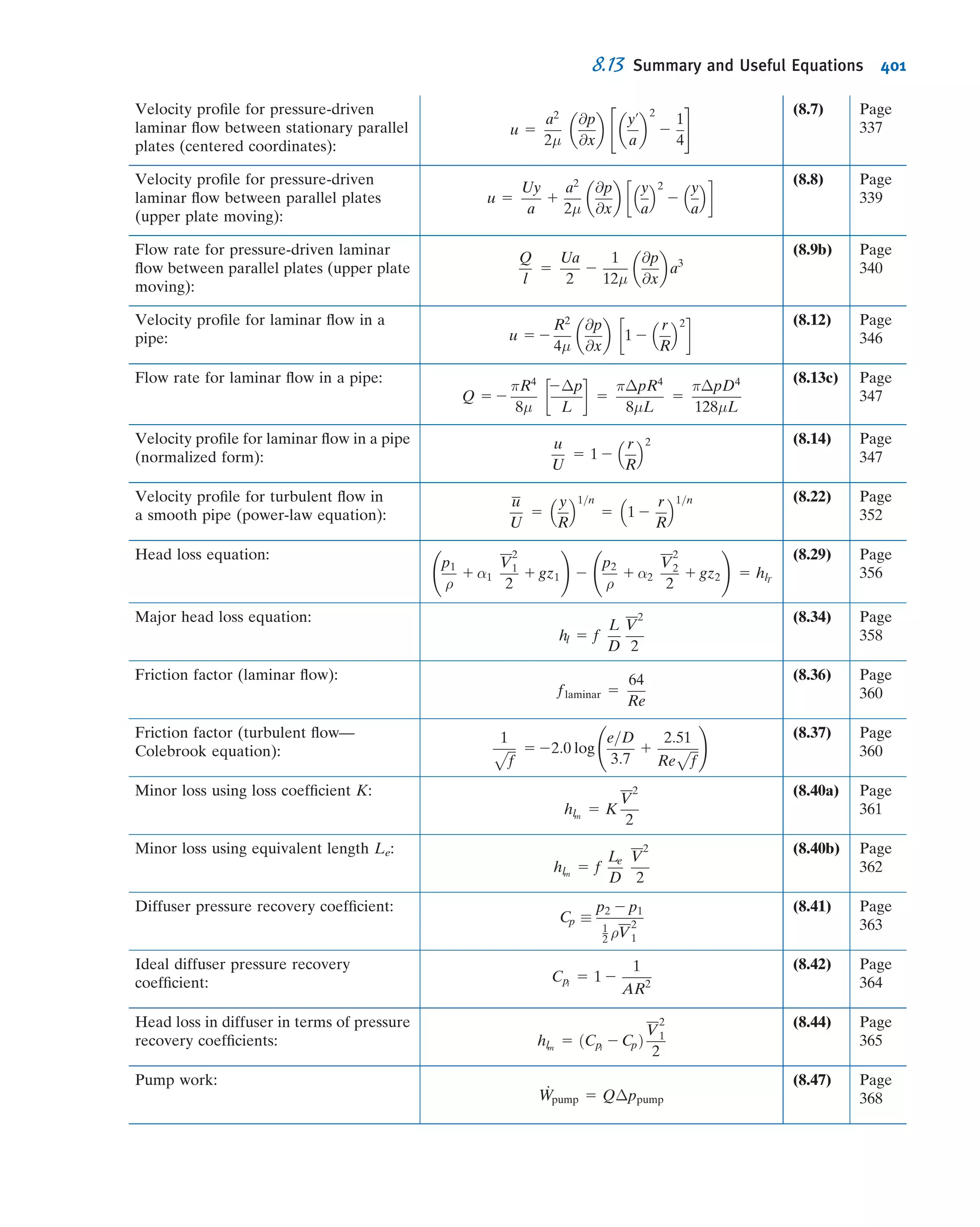


![the pipe wall. The stress on the wall, τw (equal and opposite to the stress in the fluid at
the wall), is given by
τw 5 2 τrx½ Šr 5 R 5 2
R
2
@p
@x
ð8:16Þ
For laminar flow we used our familiar stress equation τrx 5 μ du/dr in Eq. 8.15 to
eventually obtain the laminar velocity distribution. This led to a set of usable equa-
tions, Eqs. 8.13, for obtaining various flow characteristics; e.g., Eq. 8.13c gave a
relationship for the flow rate Q, a result first obtained experimentally by Jean Louis
Poiseuille, a French physician, and independently by Gotthilf H. L. Hagen, a German
engineer, in the 1850s [2].
Unfortunately there is no equivalent stress equation for turbulent flow, so we
cannot replicate the laminar flow analysis to derive turbulent equivalents of Eqs. 8.13.
All we can do in this section is indicate some classic semi-empirical results [3].
As we discussed in Section 2.6, and illustrated in Fig. 2.17, turbulent flow is repre-
sented at each point by the time-mean velocity u plus (for a two-dimensional flow)
randomly fluctuating velocity components uu and vu in the x and y directions (in this
context y is the distance inwards from the pipe wall). These components continuously
transfer momentum between adjacent fluid layers, tending to reduce any velocity
gradient present. This effect shows up as an apparent stress, first introduced by
Osborne Reynolds, and called the Reynolds stress.1
This stress is given by 2ρuuvu,
where the overbar indicates a time average. Hence, we find
τ 5 τlam 1 τturb 5 μ
du
dy
2 ρuuvu ð8:17Þ
Do not misunderstand the minus sign in Eq. 8.17—it turns out that uu and vu are
negatively correlated, so that τturb 5 2ρuuvu is positive. In Fig. 8.8, experimental
measurements of the Reynolds stress for fully developed turbulent pipe flow at two
Reynolds numbers are presented; ReU 5 UD=ν, where U is the centerline velocity.
The turbulent shear stress has been nondimensionalized with the wall shear stress.
Recall that Eq. 8.15 showed that the shear stress in the fluid varies linearly from τw
at the pipe wall (y/R - 0) to zero at the centerline (y/R 5 1); from Fig. 8.8 we see that
the Reynolds stress has almost the same trend, so that the friction is almost all due to
Reynolds stress. What Fig. 8.8 doesn’t show is that close to the wall (y/R - 0)
the Reynolds stress drops to zero. This is because the no-slip condition holds, so not
ReU
500,000
50,000
1.00.80.60.4
Dimensionless distance from wall,
0.20
0
0.2
0.4
0.6
0.8
1.0
____
– u'v'_____
τw
ρ
y___
R
Fig. 8.8 Turbulent shear stress (Reynolds stress) for fully developed
turbulent flow in a pipe. (Data from Laufer [5].)
1
The Reynolds stress terms arise from consideration of the complete equations of motion for turbulent flow [4].
350 Chapter 8 Internal Incompressible Viscous Flow](https://image.slidesharecdn.com/foxphilipj-160402150646/75/Fox-Philip-J-Pritchard-8-ed-Mc-Donald-s-Introduction-to-Fluid-Mechanics-wiley-2011-426-2048.jpg)
![only does the mean velocity u-0, but also the fluctuating velocity components uu and
vu-0 (the wall tends to suppress the fluctuations). Hence, the turbulent stress,
τturb 5 2ρuuvu-0, as we approach the wall, and is zero at the wall. Since the Reynolds
stress is zero at the wall, Eq. 8.17 shows that the wall shear is given by
τw 5 μðdu=dyÞy 5 0. In the region very close to the wall, called the wall layer, viscous
shear is dominant. In the region between the wall layer and the central portion of the
pipe both viscous and turbulent shear are important.
8.5Turbulent Velocity Profiles in Fully
Developed Pipe Flow
Except for flows of very viscous fluids in small diameter ducts, internal flows generally
are turbulent. As noted in the discussion of shear stress distribution in fully developed
pipe flow (Section 8.4), in turbulent flow there is no universal relationship between the
stress field and the mean velocity field. Thus, for turbulent flows we are forced to rely
on experimental data.
Dividing Eq. 8.17 by ρ gives
τ
ρ
5 ν
du
dy
2 uuvu ð8:18Þ
The term τ/ρ arises frequently in the consideration of turbulent flows; it has dimen-
sions of velocity squared. In particular, the quantity ðτw=ρÞ1=2
is called the friction
velocity and is denoted by the symbol u*. It is a constant for a given flow.
The velocity profile for fully developed turbulent flow through a smooth pipe is
shown in Fig. 8.9. The plot is semilogarithmic; u=u* is plotted against log(yu*=ν). The
nondimensional parameters u=u* and yu*=ν arise from dimensional analysis if one
reasons that the velocity in the neighborhood of the wall is determined by the con-
ditions at the wall, the fluid properties, and the distance from the wall. It is simply
fortuitous that the dimensionless plot of Fig. 8.9 gives a fairly accurate representation
of the velocity profile in a pipe away from the wall; note the small deviations in the
region of the pipe centerline.
ReU = 5ϫ104
ReU = 5ϫ105
(Solid points are centerline values)
104
52103
52102
5210521
0
10
20
30
_
u__
u*
_
u__
u*
=
_
u__
u*
= 2.5 ln + 5.0
yu*____
yu*
yu*____
n
n
n
Fig. 8.9 Turbulent velocity profile for fully developed flow in a smooth pipe.
(Data from Laufer [5].)
VIDEO
The Glen Canyon Dam: A Turbulent Pipe
Flow.
8.5 Turbulent Velocity Profiles in Fully Developed Pipe Flow 351](https://image.slidesharecdn.com/foxphilipj-160402150646/75/Fox-Philip-J-Pritchard-8-ed-Mc-Donald-s-Introduction-to-Fluid-Mechanics-wiley-2011-427-2048.jpg)
![In the region very close to the wall where viscous shear is dominant, the mean
velocity profile follows the linear viscous relation
u1
5
u
u*
5
yu*
ν
5y1
ð8:19Þ
where y is distance measured from the wall (y 5 R 2 r; R is the pipe radius), and u is
mean velocity. Equation 8.19 is valid for 0 # y1
# 5À7; this region is called the viscous
sublayer.
For values of yu*=ν . 30, the data are quite well represented by the semiloga-
rithmic curve-fit equation
u
u*
5 2:5 ln
yu*
ν
1 5:0 ð8:20Þ
In this region both viscous and turbulent shear are important (although turbulent
shear is expected to be significantly larger). There is considerable scatter in the
numerical constants of Eq. 8.20; the values given represent averages over many
experiments [6]. The region between y1
5 527 and y1
5 30 is referred to as the
transition region, or buffer layer.
If Eq. 8.20 is evaluated at the centerline (y 5 R and u 5 U) and the general
expression of Eq. 8.20 is subtracted from the equation evaluated at the centerline, we
obtain
U 2 u
u*
5 2:5 ln
R
y
ð8:21Þ
where U is the centerline velocity. Equation 8.21, referred to as the defect law, shows
that the velocity defect (and hence the general shape of the velocity profile in the
neighborhood of the centerline) is a function of the distance ratio only and does not
depend on the viscosity of the fluid.
The velocity profile for turbulent flow through a smooth pipe may also be
approximated by the empirical power-law equation
u
U
5
y
R
1=n
5 1 2
r
R
1=n
ð8:22Þ
where the exponent, n, varies with the Reynolds number. In Fig. 8.10 the data of
Laufer [5] are shown on a plot of ln y/R versus ln u=U. If the power-law profile were
an accurate representation of the data, all data points would fall on a straight line of
slope n. Clearly the data for ReU 5 5 3 104
deviate from the best-fit straight line in the
neighborhood of the wall.
Hence the power-law profile is not applicable close to the wall (y=R , 0:04). Since
the velocity is low in this region, the error in calculating integral quantities such as
mass, momentum, and energy fluxes at a section is relatively small. The power-law
profile gives an infinite velocity gradient at the wall and hence cannot be used in
calculations of wall shear stress. Although the profile fits the data close to the cen-
terline, it fails to give zero slope there. Despite these shortcomings, the power-law
profile is found to give adequate results in many calculations.
Data from Hinze [7] suggest that the variation of power-law exponent n with
Reynolds number (based on pipe diameter, D, and centerline velocity, U) for fully
developed flow in smooth pipes is given by
n 5 21:7 1 1:8 log ReU ð8:23Þ
for ReU . 2 3 104
.
VIDEO
Computer Simulation: Turbulent Channel
Flow 1.
VIDEO
Computer Simulation: Turbulent Channel
Flow 2.
VIDEO
Computer Simulation: Turbulent Channel
Flow 3.
352 Chapter 8 Internal Incompressible Viscous Flow](https://image.slidesharecdn.com/foxphilipj-160402150646/75/Fox-Philip-J-Pritchard-8-ed-Mc-Donald-s-Introduction-to-Fluid-Mechanics-wiley-2011-428-2048.jpg)
![Since the average velocity is V 5 Q=A, and
Q 5
Z
A
~V Á d ~A
the ratio of the average velocity to the centerline velocity may be calculated for the
power-law profiles of Eq. 8.22 assuming the profiles to be valid from wall to centerline.
The result is
V
U
5
2n2
ðn 1 1Þð2n 1 1Þ
ð8:24Þ
From Eq. 8.24, we see that as n increases (with increasing Reynolds number) the ratio
of the average velocity to the centerline velocity increases; with increasing Reynolds
number the velocity profile becomes more blunt or “fuller” (for n 5 6; V=U 5 0:79
and for n 5 10; V=U 5 0:87). As a representative value, 7 often is used for the
exponent; this gives rise to the term “a one-seventh power profile” for fully developed
turbulent flow:
u
U
5
y
R
1=7
5 1 2
r
R
1=7
Velocity profiles for n 5 6 and n 5 10 are shown in Fig. 8.11. The parabolic profile for
fully developed laminar flow is included for comparison. It is clear that the turbulent
profile has a much steeper slope near the wall. This is consistent with our discussion
leading to Eq. 8.17—the fluctuating velocity components uu and vu continuously
transfer momentum between adjacent fluid layers, tending to reduce the velocity
gradient.
8.6Energy Considerations in Pipe Flow
We have so far used the momentum and conservation of mass equations, in control
volume form, to discuss viscous flow. It is obvious that viscous effects will have an
ReU = 5ϫ104
ReU = 5ϫ105
1.00
0.50
0.20
0.10
0.05
0.02
0.01
0.005
0.002
0.10 0.20 0.50 1.00 0.50 0.70 1.00
y___
R
U
u
Fig. 8.10 Power-law velocity profiles for fully developed
turbulent flow in a smooth pipe. (Data from Laufer [5].)
8.6 Energy Considerations in Pipe Flow 353](https://image.slidesharecdn.com/foxphilipj-160402150646/75/Fox-Philip-J-Pritchard-8-ed-Mc-Donald-s-Introduction-to-Fluid-Mechanics-wiley-2011-429-2048.jpg)


![Δp
ρV
2
5 f
μ
ρVD
;
L
D
;
e
D
We recognize that μ=ρVD 5 1=Re, so we could just as well write
Δp
ρV
2
5 φ Re;
L
D
;
e
D
Substituting from Eq. 8.32, we see that
hl
V
2
5 φ Re;
L
D
;
e
D
Although dimensional analysis predicts the functional relationship, we must obtain
actual values experimentally.
Experiments show that the nondimensional head loss is directly proportional to L/D.
Hence we can write
hl
V
2
5
L
D
φ1 Re;
e
D
Since the function, φ1, is still undetermined, it is permissible to introduce a constant
into the left side of the above equation. By convention the number 1
2 is introduced into
the denominator so that the left side of the equation is the ratio of the head loss to the
kinetic energy per unit mass of flow. Then
hl
1
2 V
2
5
L
D
φ2 Re;
e
D
The unknown function, φ2ðRe; e=DÞ, is defined as the friction factor, f,
f φ2 Re;
e
D
and
hl 5 f
L
D
V
2
2
ð8:34Þ
or
Hl 5 f
L
D
V
2
2g
ð8:35Þ
The friction factor2
is determined experimentally. The results, published by L. F.
Moody [8], are shown in Fig. 8.13.
To determine head loss for fully developed flow with known conditions, the Rey-
nolds number is evaluated first. Roughness, e, is obtained from Table 8.1. Then the
friction factor, f, can be read from the appropriate curve in Fig. 8.13, at the known
values of Re and e/D. Finally, head loss can be found using Eq. 8.34 or Eq. 8.35.
2
The friction factor defined by Eq. 8.34 is the Darcy friction factor. The Fanning friction factor, less fre-
quently used, is defined in Problem 8.95.
358 Chapter 8 Internal Incompressible Viscous Flow](https://image.slidesharecdn.com/foxphilipj-160402150646/75/Fox-Philip-J-Pritchard-8-ed-Mc-Donald-s-Introduction-to-Fluid-Mechanics-wiley-2011-434-2048.jpg)
![Several features of Fig. 8.13 require some discussion. The friction factor for laminar
flow may be obtained by comparing Eqs. 8.33 and 8.34:
hl 5
64
Re
L
D
V
2
2
5 f
L
D
V
2
2
Table 8.1
Roughness for Pipes of Common Engineering Materials
Pipe
Roughness, e
Feet Millimeters
Riveted steel 0.003À0.03 0.9À9
Concrete 0.001À0.01 0.3À3
Wood stave 0.0006À0.003 0.2À0.9
Cast iron 0.00085 0.26
Galvanized iron 0.0005 0.15
Asphalted cast iron 0.0004 0.12
Commercial steel or wrought iron 0.00015 0.046
Drawn tubing 0.000005 0.0015
Source: Data from Moody [8].
Transition
zone
Fully rough zone
Smooth pipes
Recr
Laminarflowf=
64___
Re
0.1
0.09
0.08
0.07
0.06
0.05
0.04
0.03
0.025
0.02
0.015
0.01
0.009
0.008
103
104
2 3 4 5 6 8 105
2 3 4 5 6 8 106
2 3 4 5 6 8 107
2 3 4 5 6 8 108
0.000,01
0.000,05
0.0001
0.0002
0.0004
0.0006
0.0008
0.001
0.002
0.004
0.006
0.008
0.01
0.015
0.02
0.03
0.04
0.05
2 3 4 5 6 8
e___
D
= 0.000,005e___
D
e___
D
= 0.000,001Reynolds number, Re =
_
VD______ρ
μ
Frictionfactor,f
Relativeroughness,
Laminar
flow
Fig. 8.13 Friction factor for fully developed flow in circular pipes. (Data from Moody [8], used by permission.)
8.7 Calculation of Head Loss 359](https://image.slidesharecdn.com/foxphilipj-160402150646/75/Fox-Philip-J-Pritchard-8-ed-Mc-Donald-s-Introduction-to-Fluid-Mechanics-wiley-2011-435-2048.jpg)
![Consequently, for laminar flow
flaminar 5
64
Re
ð8:36Þ
Thus, in laminar flow, the friction factor is a function of Reynolds number only; it
is independent of roughness. Although we took no notice of roughness in deriving
Eq. 8.33, experimental results verify that the friction factor is a function only of
Reynolds number in laminar flow.
The Reynolds number in a pipe may be changed most easily by varying the average
flow velocity. If the flow in a pipe is originally laminar, increasing the velocity until the
critical Reynolds number is reached causes transition to occur; the laminar flow gives
way to turbulent flow. The effect of transition on the velocity profile was discussed in
Section 8.5. Figure 8.11 shows that the velocity gradient at the tube wall is much larger
for turbulent flow than for laminar flow. This change in velocity profile causes the wall
shear stress to increase sharply, with the same effect on the friction factor.
As the Reynolds number is increased above the transition value, the velocity
profile continues to become fuller, as noted in Section 8.5. For values of relative
roughness e/D # 0.001, the friction factor at first tends to follow the smooth pipe
curve, along which friction factor is a function of Reynolds number only. However, as
the Reynolds number increases, the velocity profile becomes still fuller. The size
of the thin viscous sublayer near the tube wall decreases. As roughness elements begin
to poke through this layer, the effect of roughness becomes important, and the friction
factor becomes a function of both the Reynolds number and the relative roughness.
At very large Reynolds number, most of the roughness elements on the tube wall
protrude through the viscous sublayer; the drag and, hence, the pressure loss, depend
only on the size of the roughness elements. This is termed the “fully rough” flow
regime; the friction factor depends only on e/D in this regime.
For values of relative roughness e=D $ 0:001, as the Reynolds number is increased
above the transition value, the friction factor is greater than the smooth pipe value. As
was the case for lower values of e/D, the value of Reynolds number at which the flow
regime becomes fully rough decreases with increasing relative roughness.
To summarize the preceding discussion, we see that as Reynolds number is
increased, the friction factor decreases as long as the flow remains laminar. At tran-
sition, f increases sharply. In the turbulent flow regime, the friction factor decreases
gradually and finally levels out at a constant value for large Reynolds number.
Bear in mind that the actual loss of energy is hl (Eq. 8.34), which is proportional to f
and V
2
. Hence, for laminar flow hl ~V (because f 5 64=Re, and Re~V); for the
transition region there is a sudden increase in hl; for the fully rough zone hl ~V
2
(because f % const.), and for the rest of the turbulent region hl increases at a rate
somewhere between V and V
2
. We conclude that the head loss always increases with
flow rate, and more rapidly when the flow is turbulent.
To avoid having to use a graphical method for obtaining f for turbulent flows,
various mathematical expressions have been fitted to the data. The most widely used
formula for friction factor is from Colebrook [9],
1
ffiffiffi
f
p 5 22:0 log
e=D
3:7
1
2:51
Re
ffiffiffi
f
p
!
ð8:37Þ
Equation 8.37 is implicit in f, but these days most scientific calculators have an
equation-solving feature that can be easily used to find f for a given roughness ratio e/D
and Reynolds number Re (and some calculators have the Colebrook equation itself
built in!). Certainly a spreadsheet such as Excel, or other mathematical computer
360 Chapter 8 Internal Incompressible Viscous Flow](https://image.slidesharecdn.com/foxphilipj-160402150646/75/Fox-Philip-J-Pritchard-8-ed-Mc-Donald-s-Introduction-to-Fluid-Mechanics-wiley-2011-436-2048.jpg)
![applications, can also be used (there is an Excel add-in for computing f for laminar
and turbulent flows available on the Web site). Even without using these automated
approaches, Eq. 8.37 is not difficult to solve for f—all we need to do is iterate.
Equation 8.37 is quite stable—almost any initial guess value for f in the right side will,
after very few iterations, lead to a converged value for f to three significant figures.
From Fig. 8.13, we can see that for turbulent flows f , 0.1; hence f 5 0.1 would make a
good initial value. Another strategy is to use Fig. 8.13 to obtain a good first estimate;
then usually one iteration using Eq. 8.37 yields a good value for f. As an alternative,
Haaland [10] developed the following equation,
1
ffiffiffi
f
p 5 21:8 log
e=D
3:7
1:11
1
6:9
Re
#
as an approximation to the Colebrook equation; for Re . 3000, it gives results within
about 2 percent of the Colebrook equation, without the need to iterate.
For turbulent flow in smooth pipes, the Blasius correlation, valid for Re # l05
, is
f 5
0:316
Re0:25
ð8:38Þ
When this relation is combined with the expression for wall shear stress (Eq. 8.16), the
expression for head loss (Eq. 8.32), and the definition of friction factor (Eq. 8.34), a
useful expression for the wall shear stress is obtained as
τw 5 0:0332ρV
2 ν
RV
0:25
ð8:39Þ
This equation will be used later in our study of turbulent boundary-layer flow over a
flat plate (Chapter 9).
All of the e values given in Table 8.1 are for new pipes, in relatively good condition.
Over long periods of service, corrosion takes place and, particularly in hard water
areas, lime deposits and rust scale form on pipe walls. Corrosion can weaken pipes,
eventually leading to failure. Deposit formation increases wall roughness appreciably,
and also decreases the effective diameter. These factors combine to cause e/D to
increase by factors of 5 to 10 for old pipes (see Problem 10.63). An example is shown
in Fig. 8.14.
Curves presented in Fig. 8.13 represent average values for data obtained from
numerous experiments. The curves should be considered accurate within approxi-
mately 610 percent, which is sufficient for many engineering analyses. If more
accuracy is needed, actual test data should be used.
Minor Losses
The flow in a piping system may be required to pass through a variety of fittings,
bends, or abrupt changes in area. Additional head losses are encountered, primarily as
a result of flow separation. (Energy eventually is dissipated by violent mixing in
the separated zones.) These losses will be minor (hence the term minor losses) if the
piping system includes long lengths of constant-area pipe. Depending on the device,
minor losses traditionally are computed in one of two ways, either
hlm
5 K
V
2
2
ð8:40aÞ
8.7 Calculation of Head Loss 361](https://image.slidesharecdn.com/foxphilipj-160402150646/75/Fox-Philip-J-Pritchard-8-ed-Mc-Donald-s-Introduction-to-Fluid-Mechanics-wiley-2011-437-2048.jpg)

![to 1 for turbulent flow. No improvement in minor loss coefficient for an exit is possible;
however, addition of a diffuser can reduce V
2
=2 and therefore hlm
considerably (see
Example 8.10).
b. Enlargements and Contractions
Minor loss coefficients for sudden expansions and contractions in circular ducts are
given in Fig. 8.15. Note that both loss coefficients are based on the larger V2
/2. Thus
losses for a sudden expansion are based on V
2
1=2, and those for a contraction are based
on V
2
2=2.
Losses caused by area change can be reduced somewhat by installing a nozzle or
diffuser between the two sections of straight pipe. Data for nozzles are given in Table 8.3.
Note that the final column (data for the included angle θ 5 180
) agrees with the data of
Fig. 8.15.
Losses in diffusers depend on a number of geometric and flow variables. Diffuser
data most commonly are presented in terms of a pressure recovery coefficient, Cp,
defined as the ratio of static pressure rise to inlet dynamic pressure,
Cp
p2 2 p1
1
2 ρV
2
1
ð8:41Þ
Table 8.2
Minor Loss Coefficients for Pipe Entrances
Entrance Type Minor Loss Coefficient, Ka
r
D
Reentrant
Square-edged
Rounded
0.78
0.5
r=D 0:02 0:06 $ 0:15
K 0:28 0:15 0:04
a
Based on hlm
5 K(V2
/2), where V is the mean velocity in the pipe.
Source: Data from Reference [11].
A1 A2 A1 A2
Contraction Expansion
AR = A2/A1 AR = A1/A2
1.0
0.8
0.6
0.4
0.2
0
0 0.2 0.4 0.6 0.8 1.0
0
0.2
0.4
0.6
0.8
1.0
[[hlm
=Ke
V1___
2
2
_Expansionlosscoefficient,Ke
[[hlm
=Kc
V2___
2
2
_Contractionlosscoefficient,Kc
Area ratio, AR
Fig. 8.15 Loss coefficients for flow through sudden area changes.
(Data from Streeter [1].)
8.7 Calculation of Head Loss 363](https://image.slidesharecdn.com/foxphilipj-160402150646/75/Fox-Philip-J-Pritchard-8-ed-Mc-Donald-s-Introduction-to-Fluid-Mechanics-wiley-2011-439-2048.jpg)
![This shows what fraction of the inlet kinetic energy shows up as a pressure rise. It is
not difficult to show (using the Bernoulli and continuity equations; see Problem 8.201)
that the ideal (frictionless) pressure recovery coefficient is given by
Cpi
5 1 2
1
AR2
ð8:42Þ
where AR is the area ratio. Hence, the ideal pressure recovery coefficient is a function
only of the area ratio. In reality a diffuser typically has turbulent flow, and the static
pressure rise in the direction of flow may cause flow separation from the walls if the
diffuser is poorly designed; flow pulsations can even occur. For these reasons
the actual Cp will be somewhat less than indicated by Eq. 8.42. For example, data for
conical diffusers with fully developed turbulent pipe flow at the inlet are presented in
Fig. 8.16 as a function of geometry. Note that more tapered diffusers (small diver-
gence angle φ or large dimensionless length N/R1) are more likely to approach the
ideal constant value for Cp. As we make the cone shorter, for a given fixed area ratio
we start to see a drop in Cp—we can consider the cone length at which this starts to
happen the optimum length (it is the shortest length for which we obtain the max-
imum coefficient for a given area ratio—closest to that predicted by Eq. 8.42). We can
relate Cp to the head loss. If gravity is neglected, and α1 5 α2 5 1.0, the head loss
equation, Eq. 8.29, reduces to
p1
ρ
1
V
2
1
2
#
2
p2
ρ
1
V
2
2
2
#
5 hlT
5 hlm
Thus,
hlm
5
V
2
1
2
2
V
2
2
2
2
p2 2 p1
ρ
hlm
5
V
2
1
2
1 2
V
2
2
V
2
1
!
2
p2 2 p1
1
2
ρV
2
1
#
5
V
2
1
2
1 2
V
2
2
V
2
1
!
2 Cp
#
From continuity, A1V1 5 A2V2, so
hlm
5
V
2
1
2
1 2
A1
A2
2
2 Cp
#
Table 8.3
Loss Coefficients (K) for Gradual Contractions: Round and Rectangular Ducts
Included Angle, θ, Degrees
A2/A1 10 15À40 50À60 90 120 150 180
θ
Flow
A1
A2 0.50 0.05 0.05 0.06 0.12 0.18 0.24 0.26
0.25 0.05 0.04 0.07 0.17 0.27 0.35 0.41
0.10 0.05 0.05 0.08 0.19 0.29 0.37 0.43
Note: Coefficients are based on hlm
5 Kð ~V
2
2=2Þ.
Source: Data from ASHRAE [12].
364 Chapter 8 Internal Incompressible Viscous Flow](https://image.slidesharecdn.com/foxphilipj-160402150646/75/Fox-Philip-J-Pritchard-8-ed-Mc-Donald-s-Introduction-to-Fluid-Mechanics-wiley-2011-440-2048.jpg)
![or
hlm
5
V
2
1
2
1 2
1
ðARÞ2
!
2 Cp
#
ð8:43Þ
The frictionless result (Eq. 8.42) is obtained from Eq. 8.43 if hlm
5 0. We can combine
Eqs. 8.42 and 8.43 to obtain an expression for the head loss in terms of the actual and
ideal Cp values:
hlm
5 ðCpi
2 CpÞ
V
2
1
2
ð8:44Þ
Performance maps for plane wall and annular diffusers [14] and for radial diffusers
[15] are available in the literature.
Diffuser pressure recovery is essentially independent of Reynolds number for inlet
Reynolds numbers greater than 7.5 3 104
[16]. Diffuser pressure recovery with uni-
form inlet flow is somewhat better than that for fully developed inlet flow. Perfor-
mance maps for plane wall, conical, and annular diffusers for a variety of inlet flow
conditions are presented in [17].
Since static pressure rises in the direction of flow in a diffuser, flow may separate
from the walls. For some geometries, the outlet flow is distorted. For wide angle dif-
fusers, vanes or splitters can be used to suppress stall and improve pressure
recovery [18].
c. Pipe Bends
The head loss of a bend is larger than for fully developed flow through a straight
section of equal length. The additional loss is primarily the result of secondary flow,
and is represented most conveniently by an equivalent length of straight pipe. The
equivalent length depends on the relative radius of curvature of the bend, as shown in
Flow
R1
N
p1 p2
φ
φAR = (1 + tan )2N___
R1
4.0
3.0
2.0
1.8
1.6
1.4
1.3
1.2
0.5 1.0 1.5 2.0 3.0 5.0 10.08.04.00.8
Dimensionless length, N/R1
4681214
16
18
0.30
0.40
0.30
0.35
0.40
0.45
0.50
0.60
0.70
Cp = 0.35
Cp
2
=
5
degrees
φ
2
=
15
degrees
φ
2
=
20
degrees
φ
φ2
=
10
degrees
4
6
812
Arearatio,AR=A2/A1
Fig. 8.16 Pressure recovery for conical diffusers with fully developed turbulent
pipe flow at inlet. (Data from Cockrell and Bradley [13].)
CLASSIC VIDEO
Flow Visualization.
8.7 Calculation of Head Loss 365](https://image.slidesharecdn.com/foxphilipj-160402150646/75/Fox-Philip-J-Pritchard-8-ed-Mc-Donald-s-Introduction-to-Fluid-Mechanics-wiley-2011-441-2048.jpg)
![Fig. 8.17a for 90
bends. An approximate procedure for computing the resistance of
bends with other turning angles is given in [11].
Because they are simple and inexpensive to construct in the field, miter bends often
are used in large pipe systems. Design data for miter bends are given in Fig. 8.17b.
Note that you get what you pay for: From Fig. 8.17a the equivalent length for pipe
bends varies from about 10 to about 40 diameters; for the cheaper 90
miter bend of
Fig. 8.17b we get a much larger equivalent length of 60 diameters.
d. Valves and Fittings
Losses for flow through valves and fittings also may be expressed in terms of an
equivalent length of straight pipe. Some representative data are given in Table 8.4.
All resistances are given for fully open valves; losses increase markedly when
valves are partially open. Valve design varies significantly among manufacturers.
40
30
20
10
0 5 10
Relative radius, r/D
(a)
15
Dimensionlessequivalentlength,Le/D
r
D
60
40
20
0
0 30 4515 60 75
Deflection angle, (degrees)
(b)
90
Dimensionlessequivalentlength,Le/D
D
D D
θ
θ
Fig. 8.17 Representative total resistance (Le/D) for (a) 90
pipe bends and flanged elbows,
and (b) miter bends. (Data from Reference [11].)
Table 8.4
Representative Dimensionless Equivalent Lengths (Le/D) for Valves and
Fittings
Fitting Type Equivalent Length,a
Le/D
Valves (fully open)
Gate valve 8
Globe valve 340
Angle valve 150
Ball valve 3
Lift check valve: globe lift 600
angle lift 55
Foot valve with strainer: poppet disk 420
hinged disk 75
Standard elbow: 90
30
45
16
Return bend, close pattern 50
Standard tee: flow through run 20
flow through branch 60
a
Based on hlm
5 fðLe=DÞðV
2
=2Þ.
Source: Data from Reference [11].
366 Chapter 8 Internal Incompressible Viscous Flow](https://image.slidesharecdn.com/foxphilipj-160402150646/75/Fox-Philip-J-Pritchard-8-ed-Mc-Donald-s-Introduction-to-Fluid-Mechanics-wiley-2011-442-2048.jpg)


![from sheet metal, they are commonly used in air conditioning, heating, and ventilating
applications. Extensive data on losses for air flow are available (e.g., see [12, 19]).
Losses caused by secondary flows increase rapidly for more extreme geometries, so
the correlations are not applicable to wide, flat ducts, or to ducts of triangular or other
irregular shapes. Experimental data must be used when precise design information is
required for specific situations.
8.8Solution of Pipe Flow Problems
Section 8.7 provides us with a complete scheme for solving many different pipe flow
problems. For convenience we collect together the relevant computing equations.
The energy equation, relating the conditions at any two points 1 and 2 for a single-
path pipe system, is
p1
ρ
1 α1
V
2
1
2
1 gz1
!
2
p2
ρ
1 α2
V
2
2
2
1 gz2
!
5 hlT
5
X
hl 1
X
hlm
ð8:29Þ
This equation expresses the fact that there will be a loss of mechanical energy
(“pressure,” kinetic and/or potential) in the pipe. Recall that for turbulent flows α % 1.
Note that by judicious choice of points 1 and 2 we can analyze not only the entire pipe
system, but also just a certain section of it that we may be interested in. The total head
loss is given by the sum of the major and minor losses. (Remember that we can also
include “negative losses” for any pumps present between points 1 and 2. The relevant
form of the energy equation is then Eq. 8.49.)
Each major loss is given by
hl 5 f
L
D
V
2
2
ð8:34Þ
where the friction factor is obtained from
f 5
64
Re
for laminar flow ðRe , 2300Þ ð8:36Þ
or
1
ffiffiffi
f
p 5 22:0 log
e=D
3:7
1
2:51
Re
ffiffiffi
f
p
!
for turbulent flow ðRe $ 2300Þ ð8:37Þ
and Eqs. 8.36 and 8.37 are presented graphically in the Moody chart (Fig. 8.13).
Each minor loss is given either by
hlm
5 K
V
2
2
ð8:40aÞ
where K is the device loss coefficient, or
hlm
5 f
Le
D
V
2
2
ð8:40bÞ
where Le is the additional equivalent length of pipe.
We also note that the flow rate Q is related to the average velocity V at each pipe
cross section by
Q 5 π
D2
4
V
We will apply these equations first to single-path systems.
8.8 Solution of Pipe Flow Problems 369](https://image.slidesharecdn.com/foxphilipj-160402150646/75/Fox-Philip-J-Pritchard-8-ed-Mc-Donald-s-Introduction-to-Fluid-Mechanics-wiley-2011-445-2048.jpg)


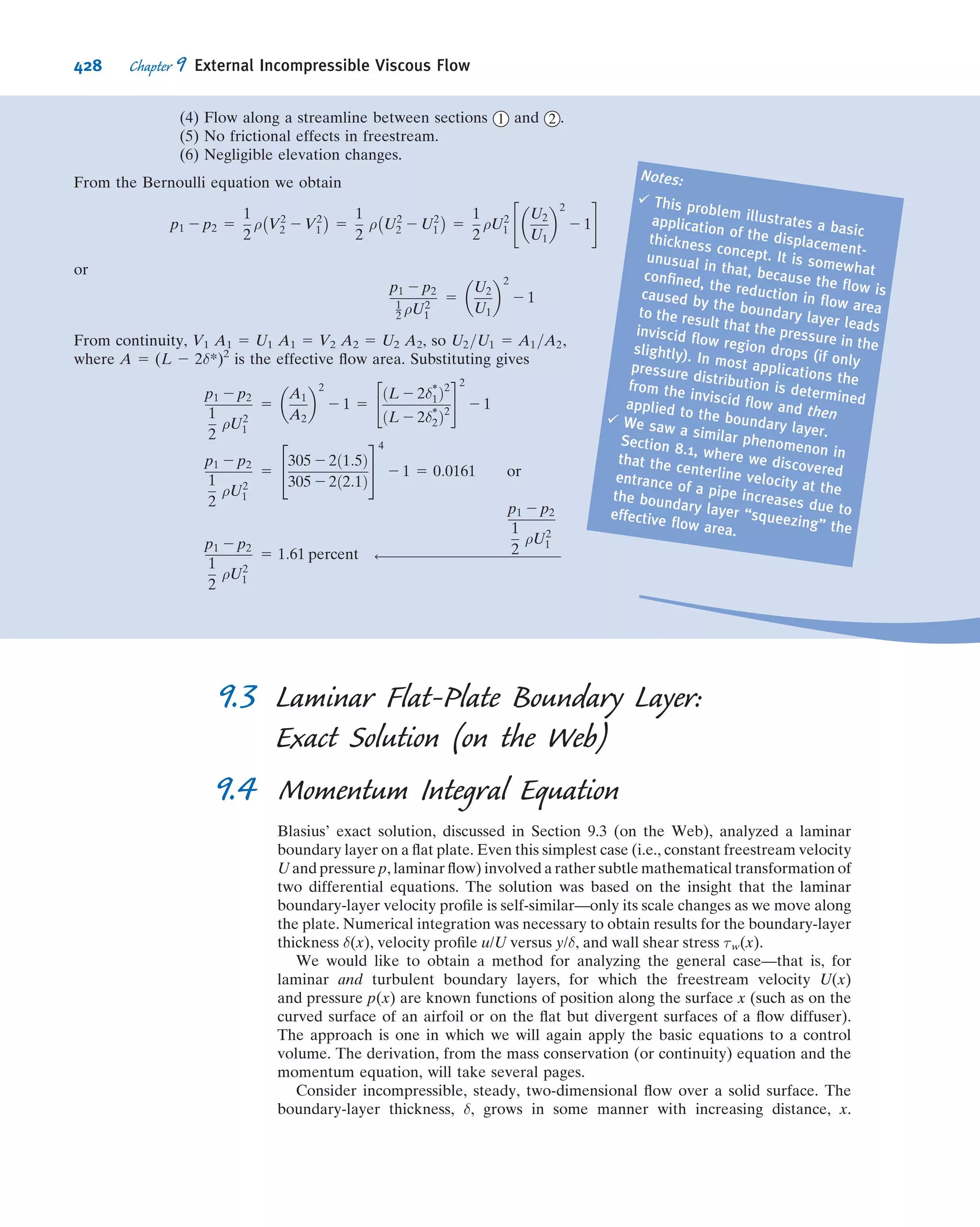
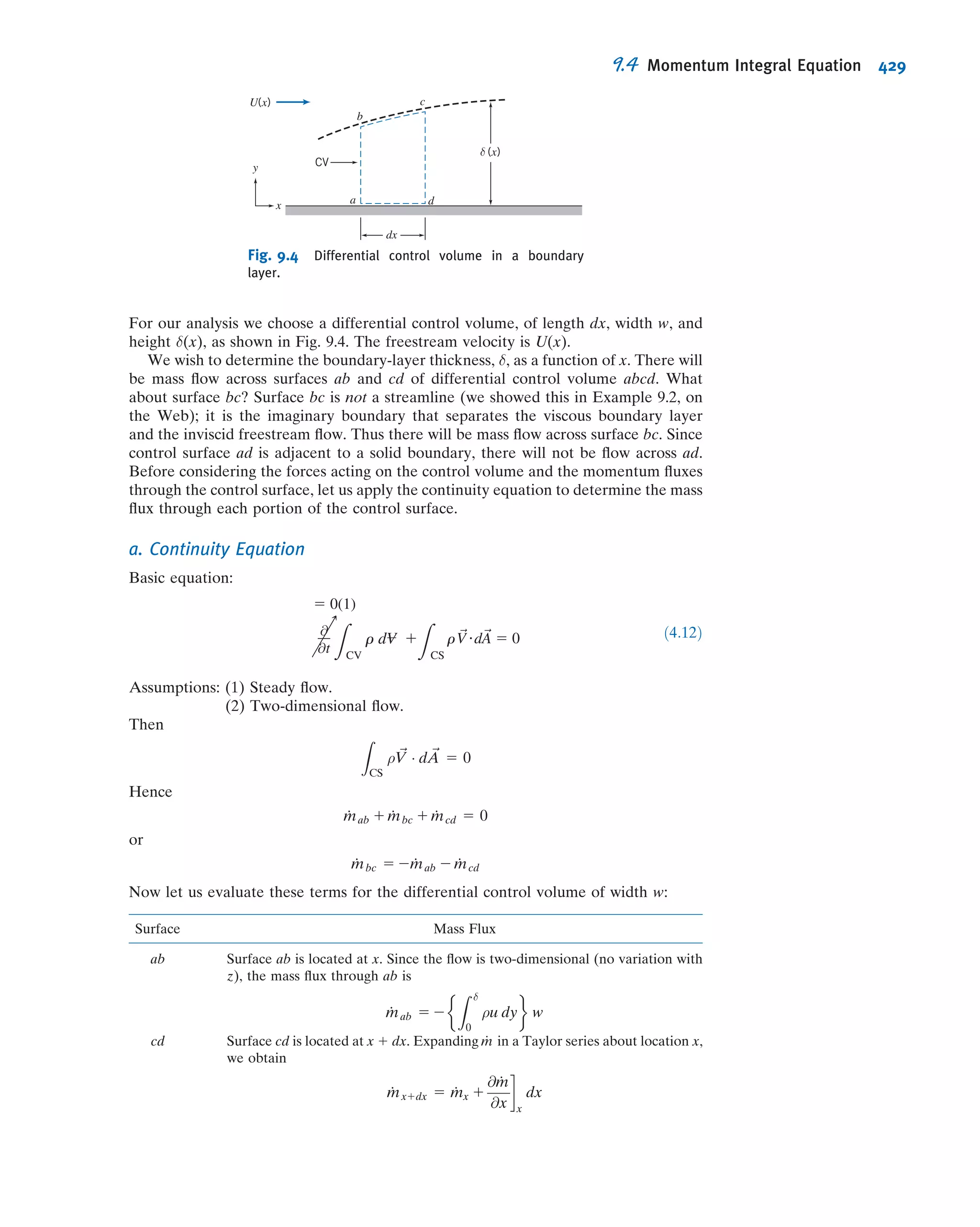


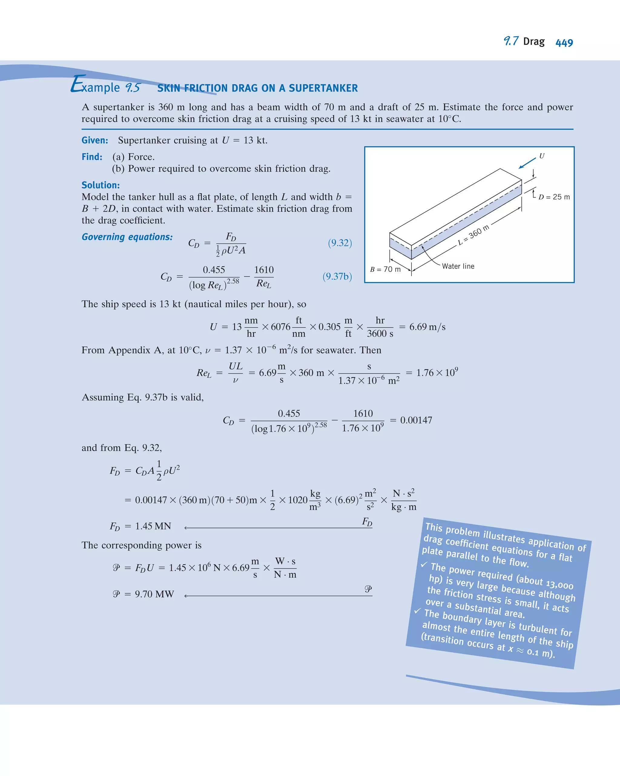


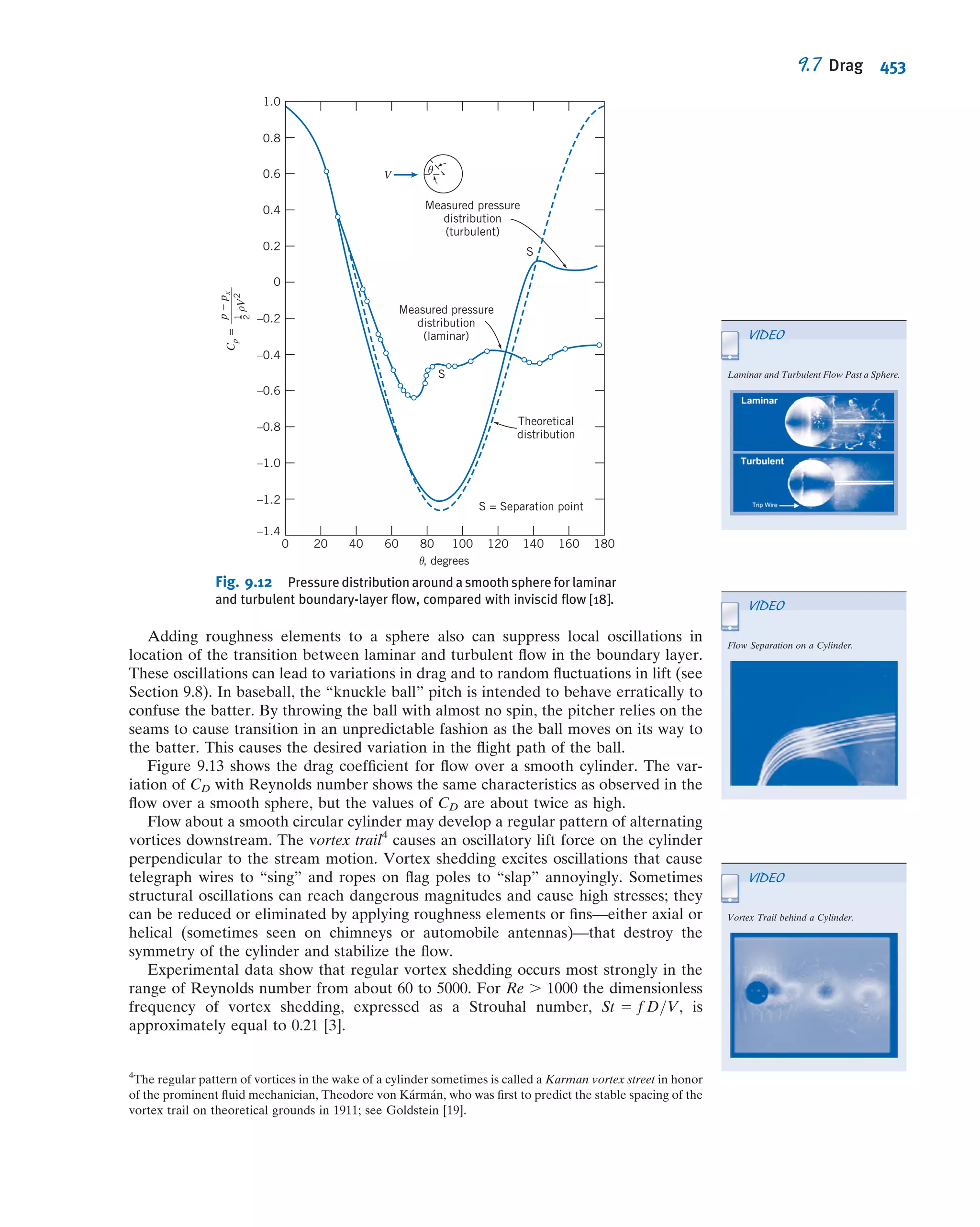
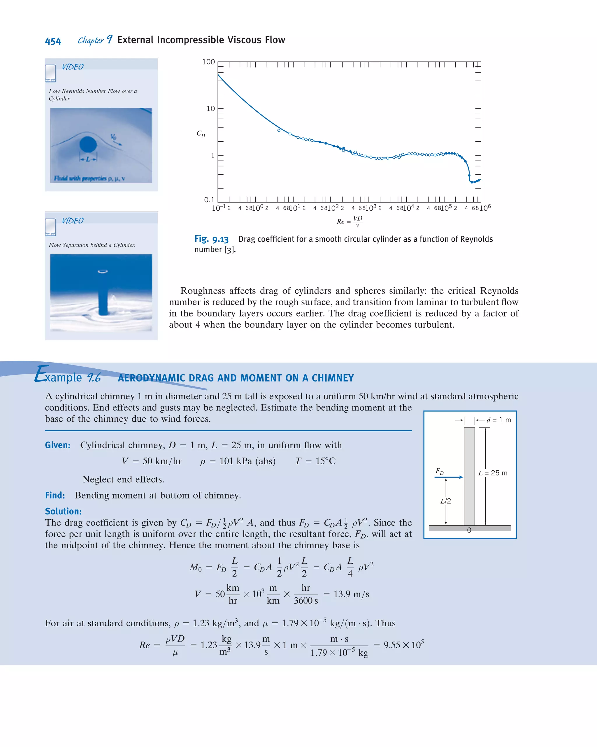

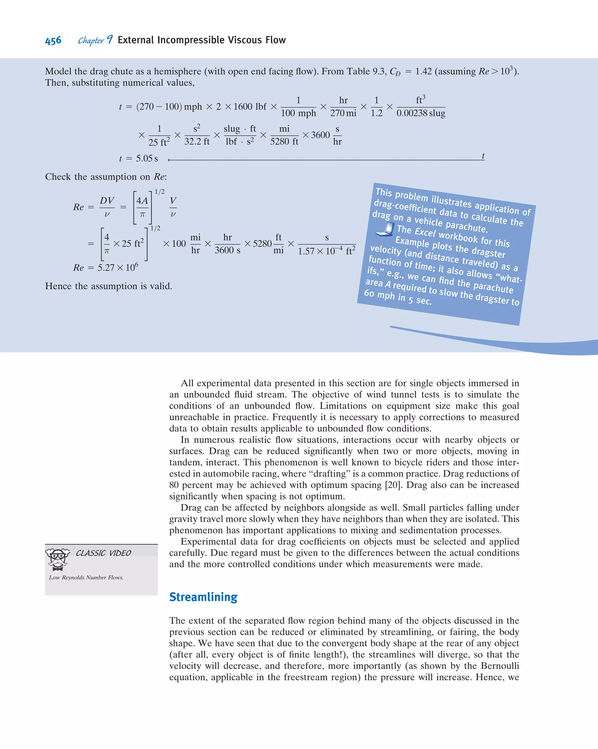


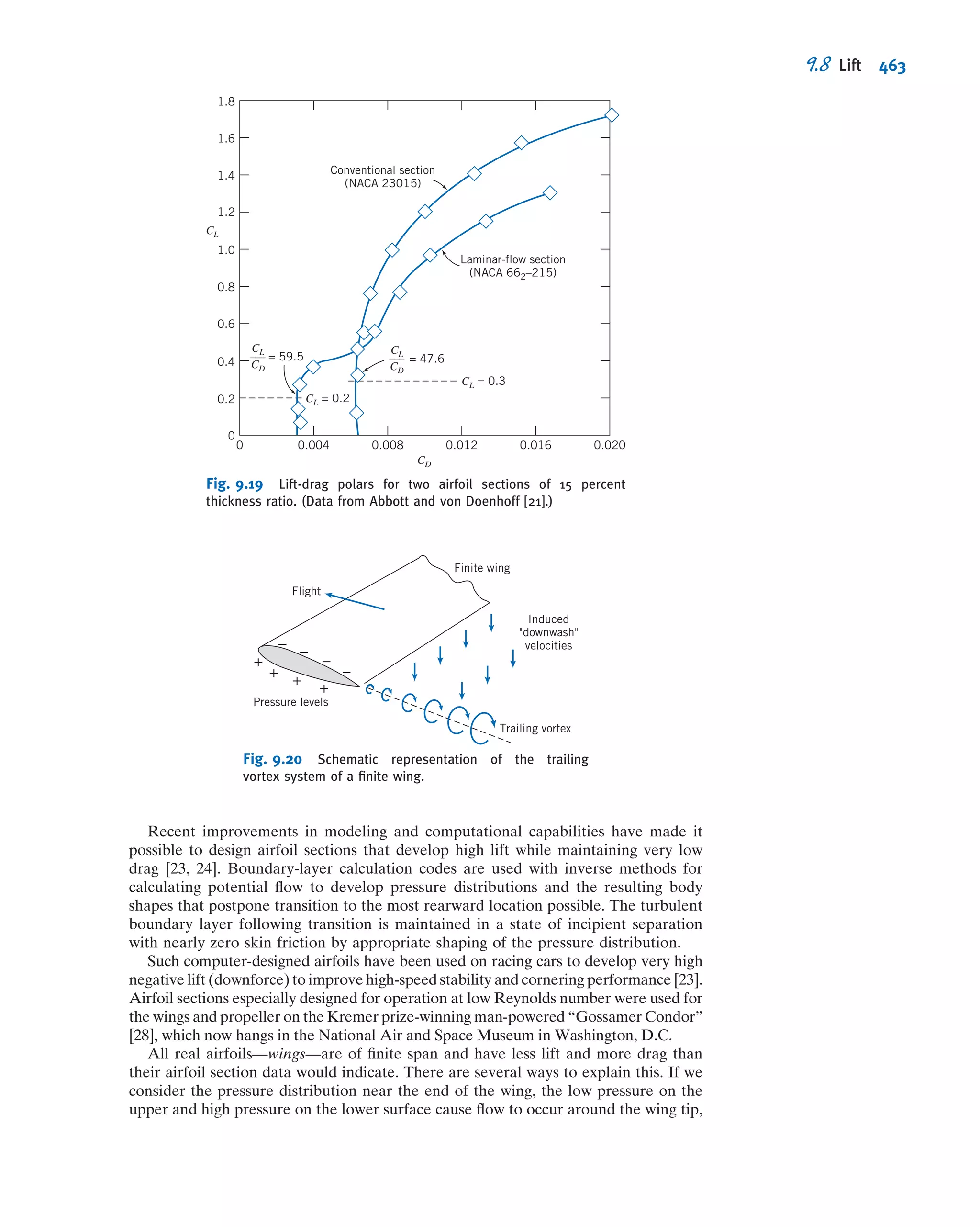
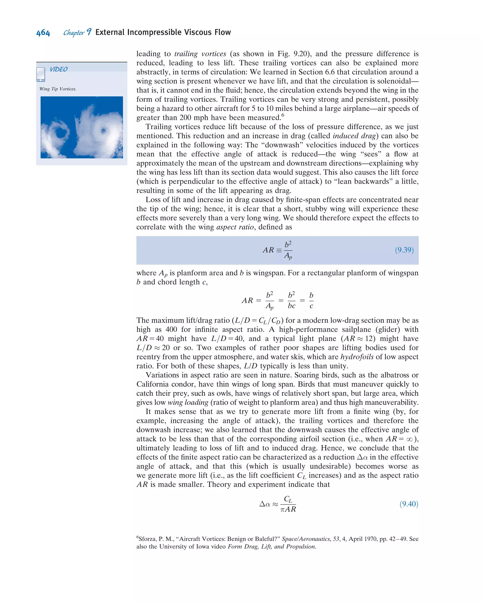


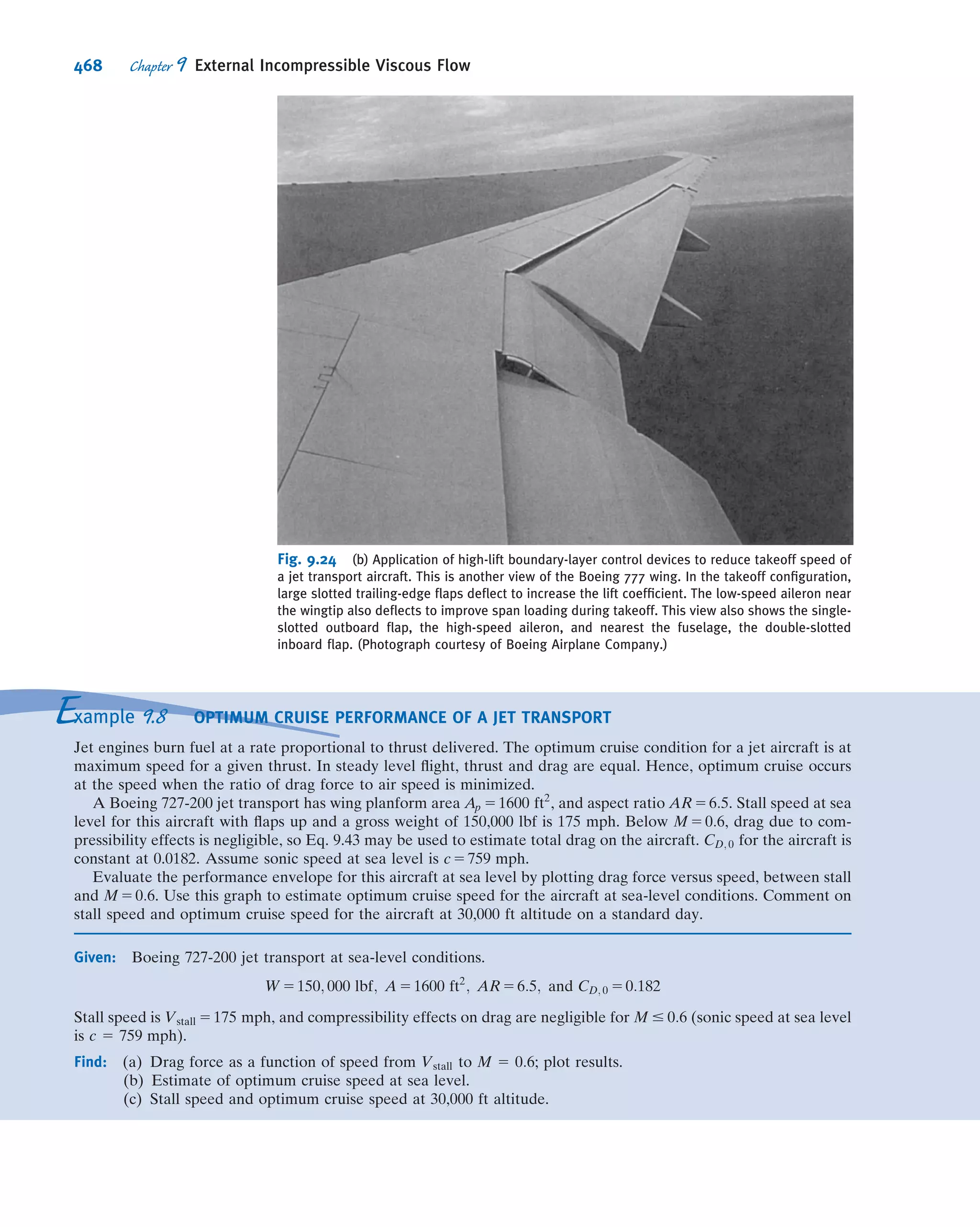


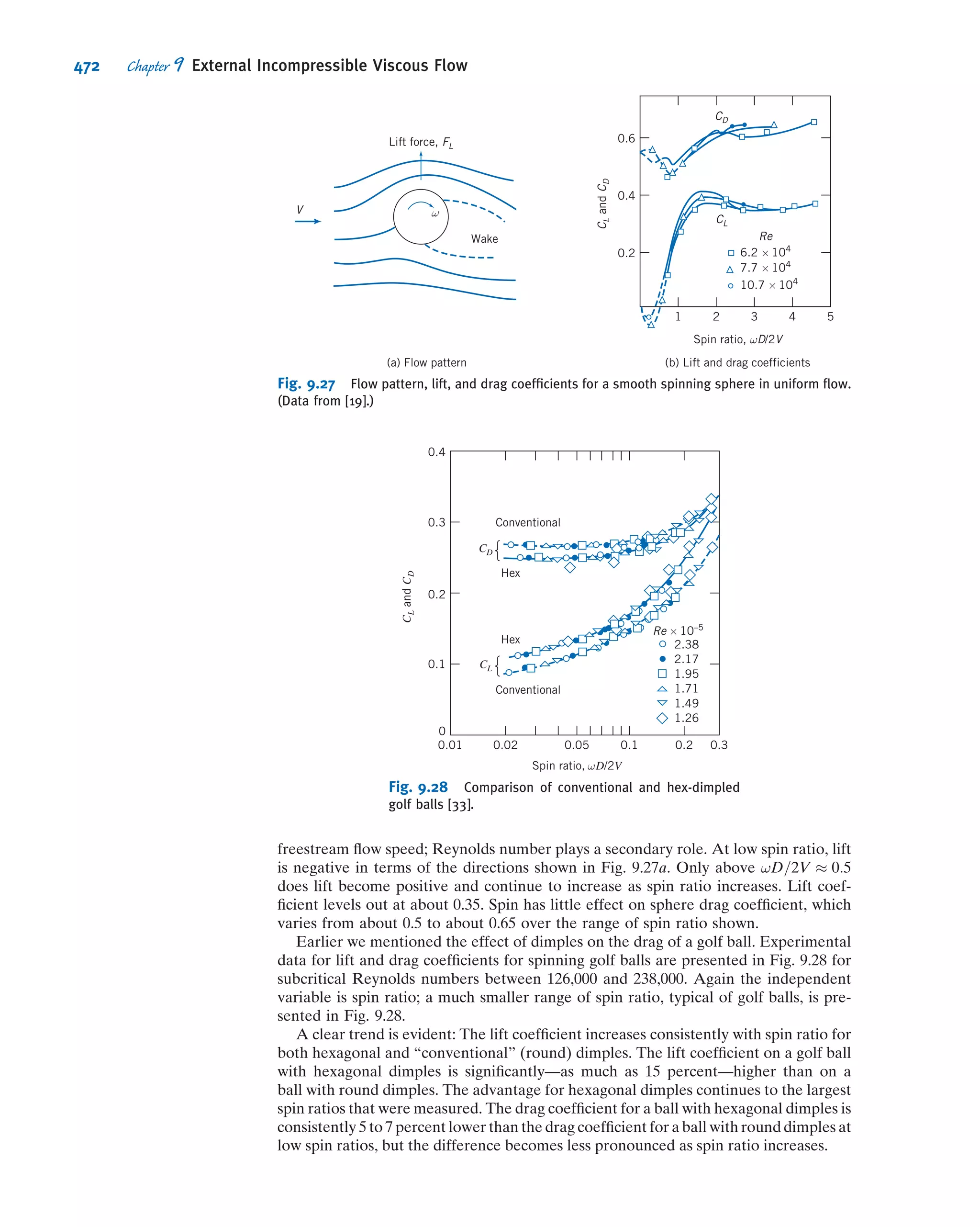


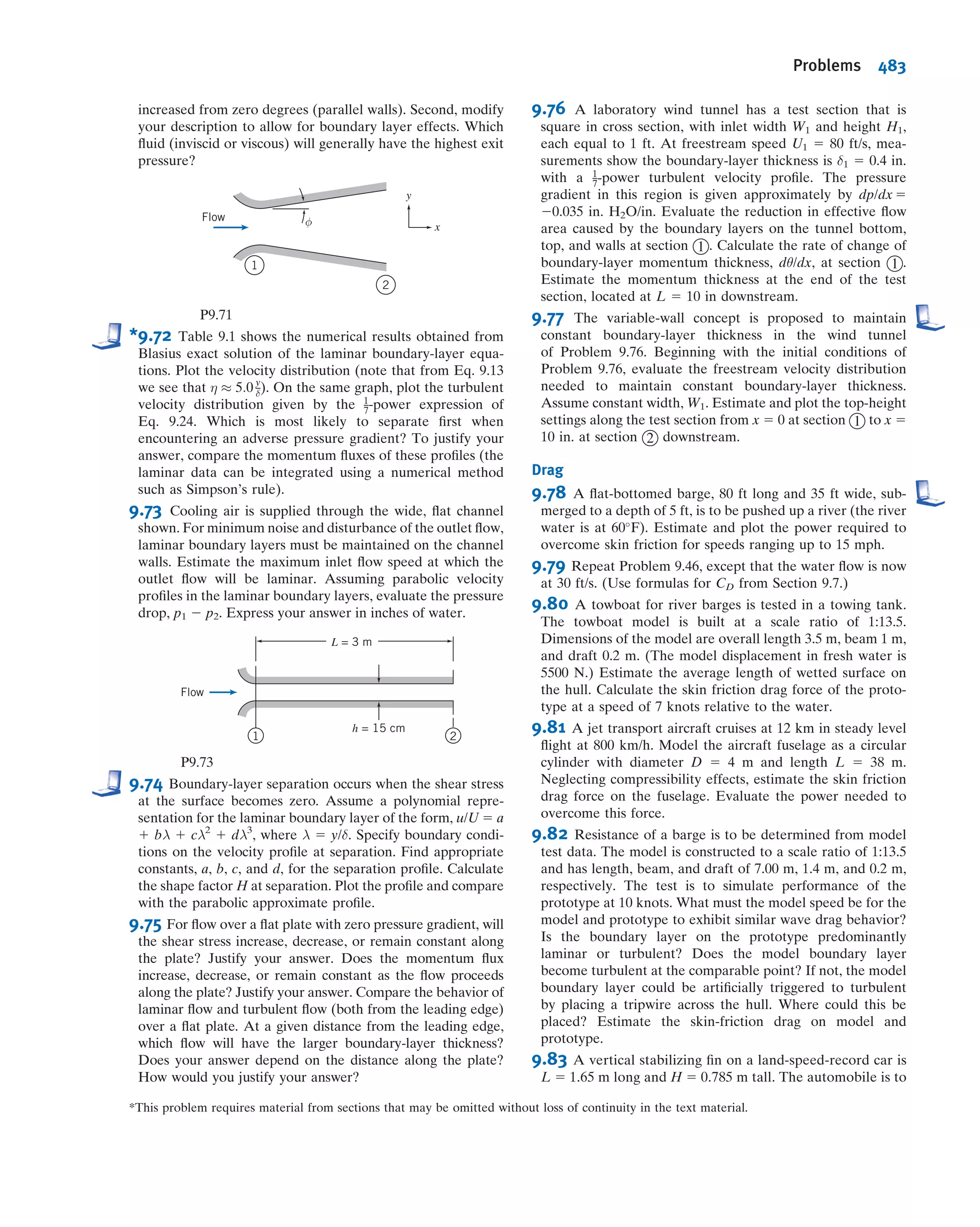


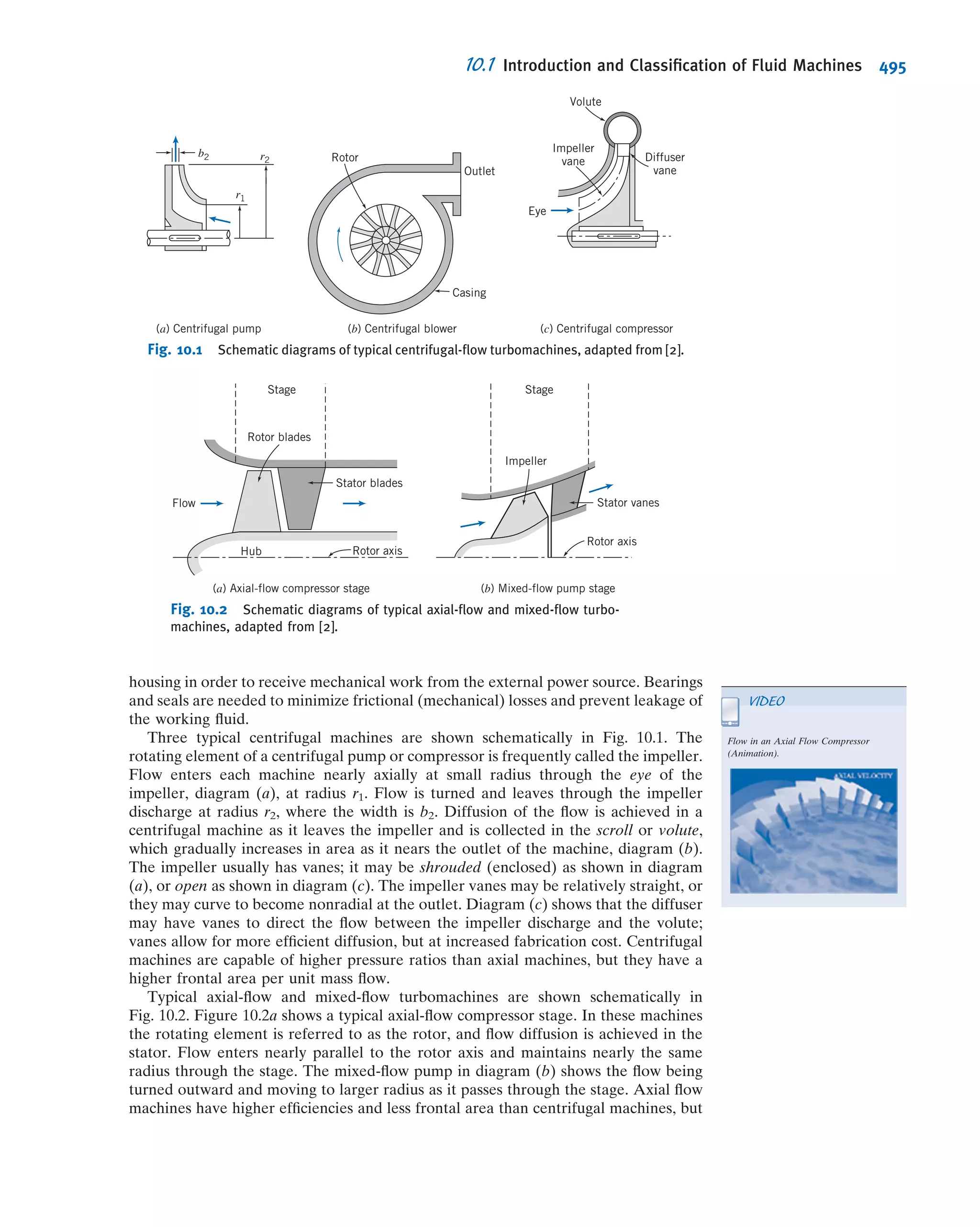
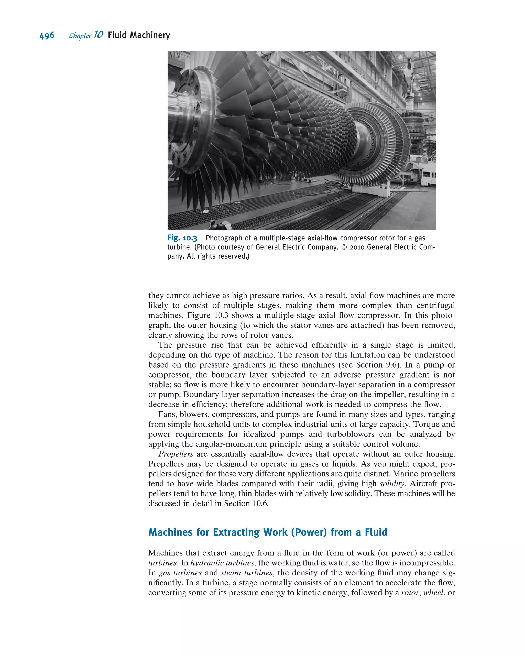

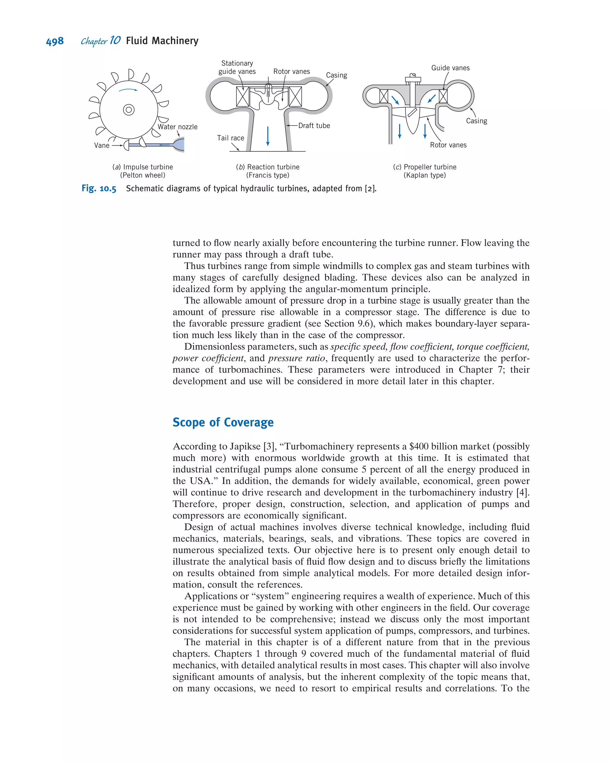


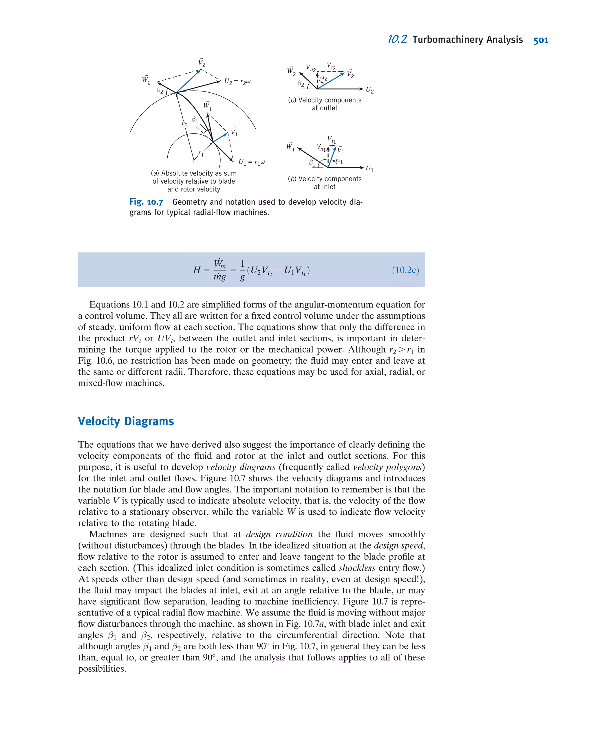
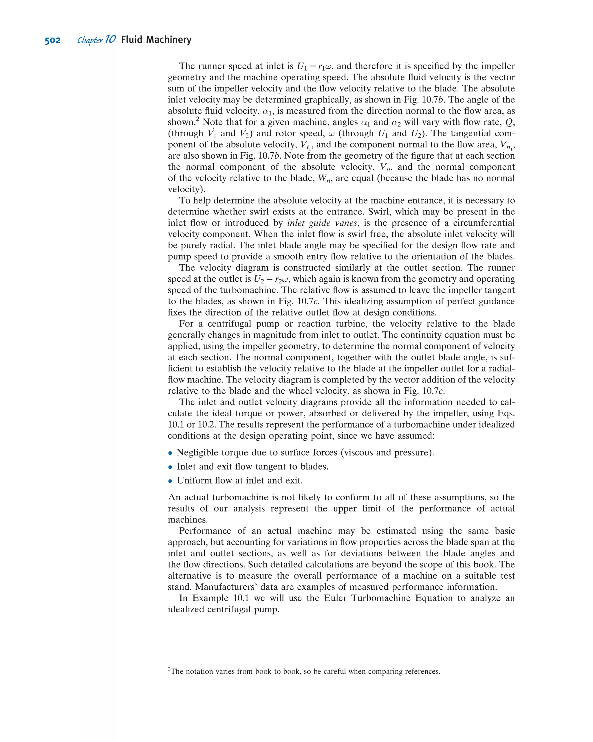
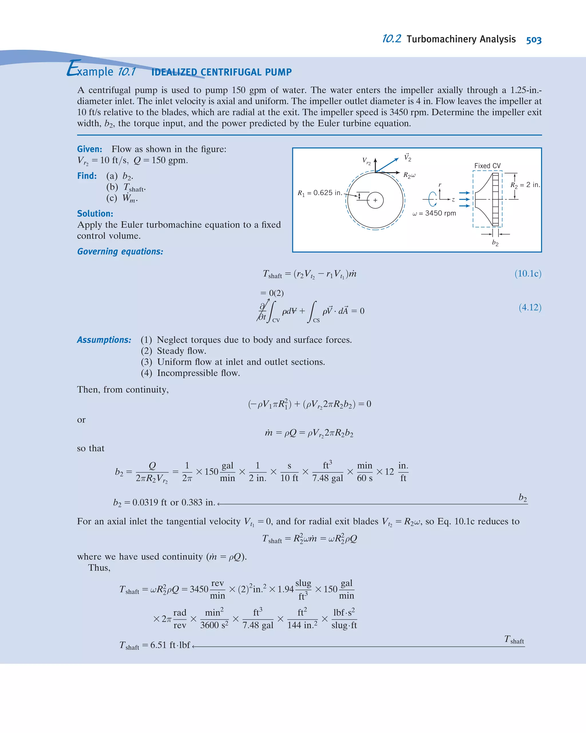


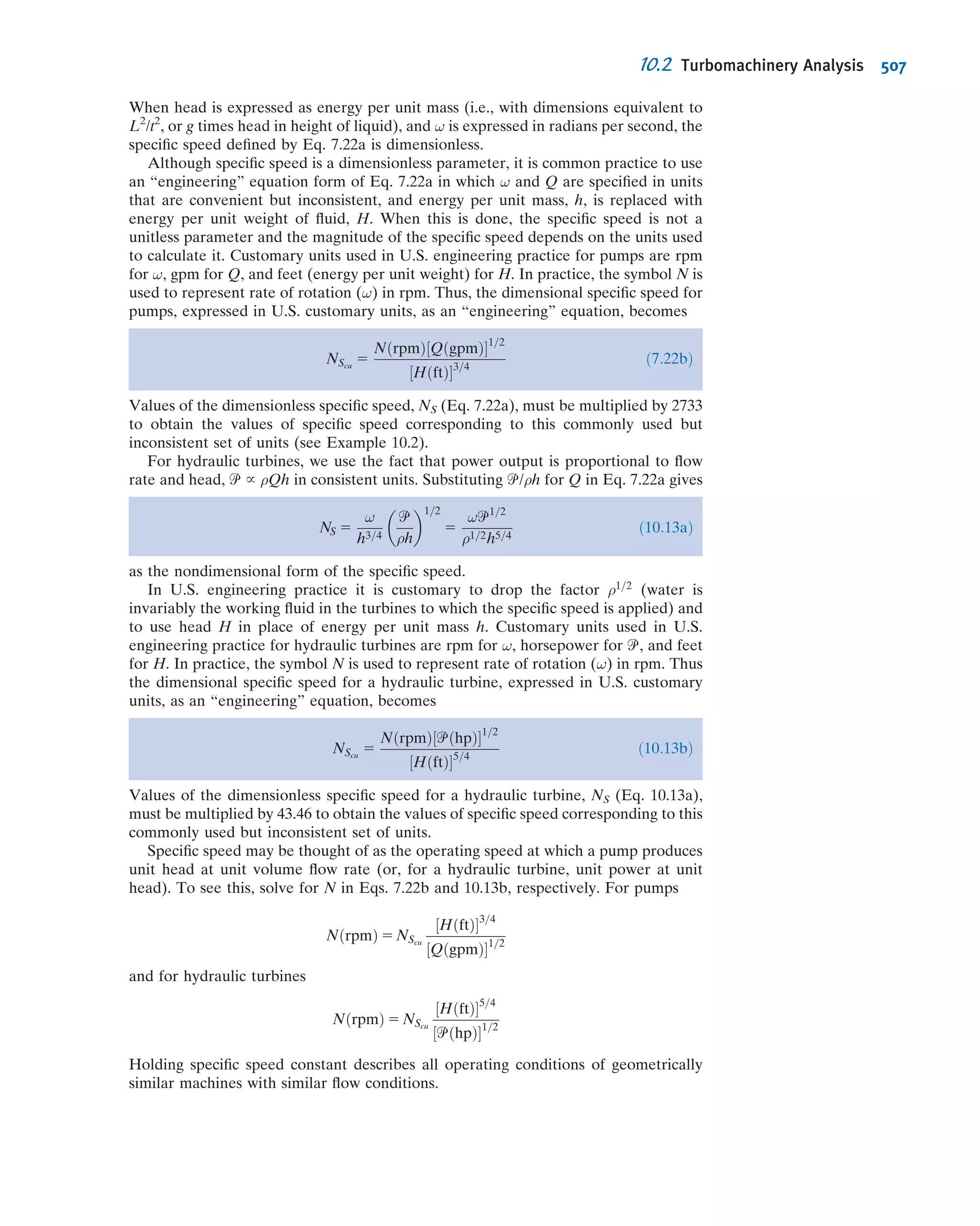
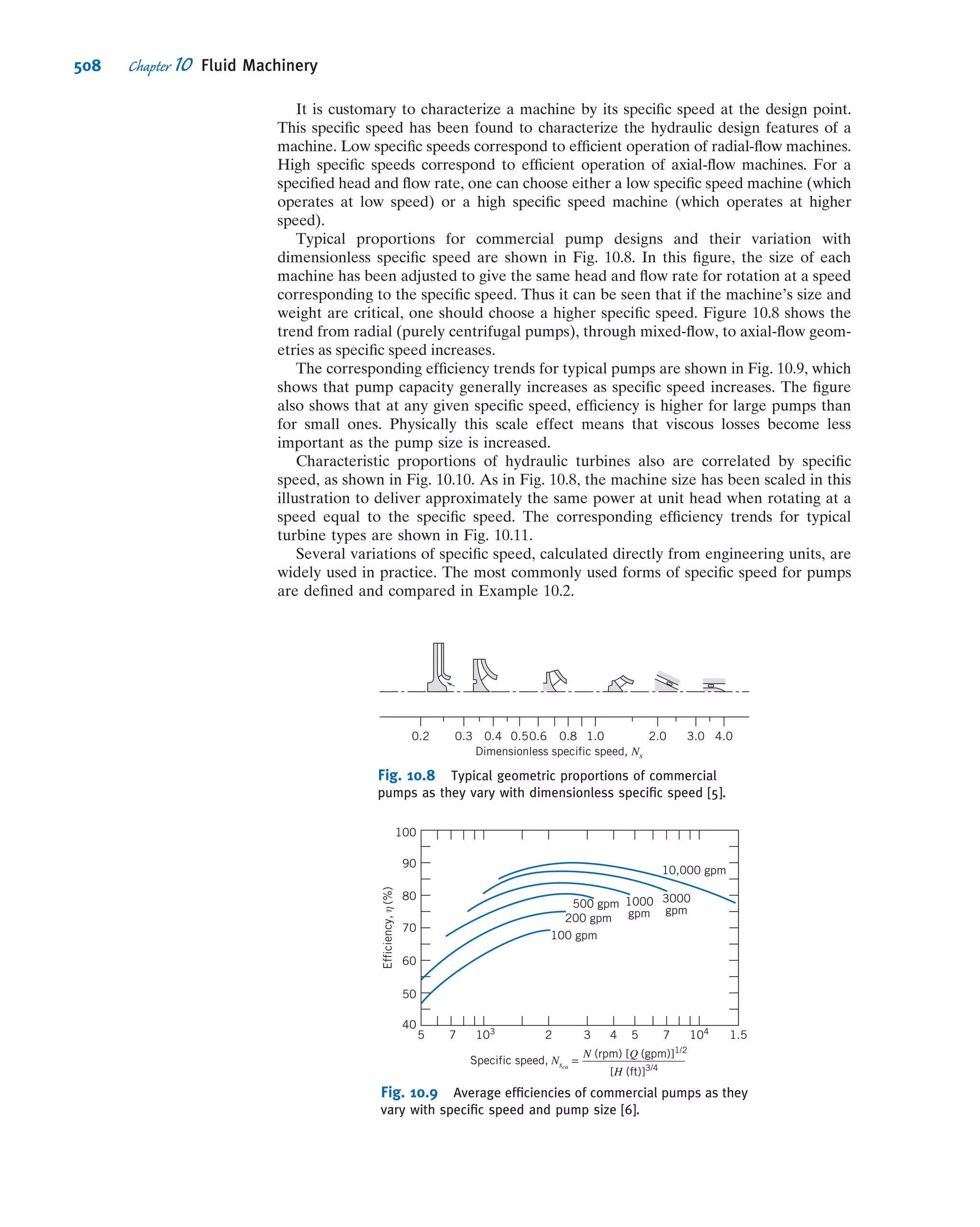
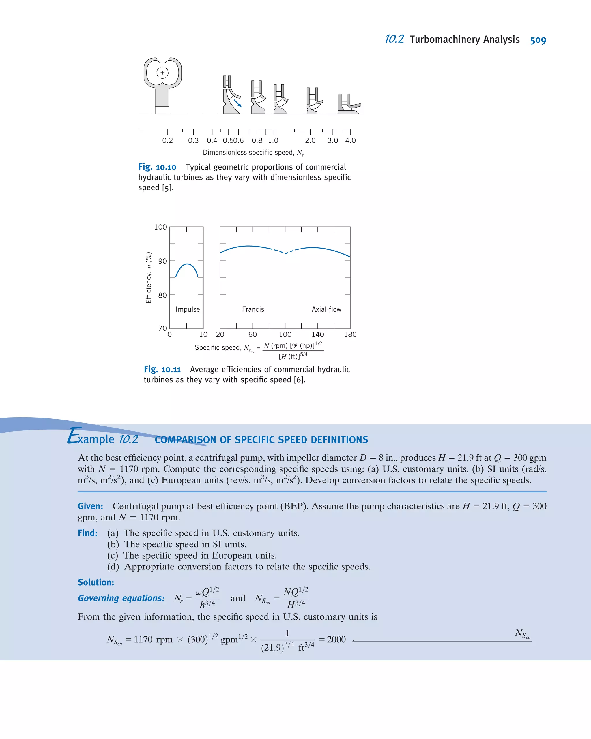
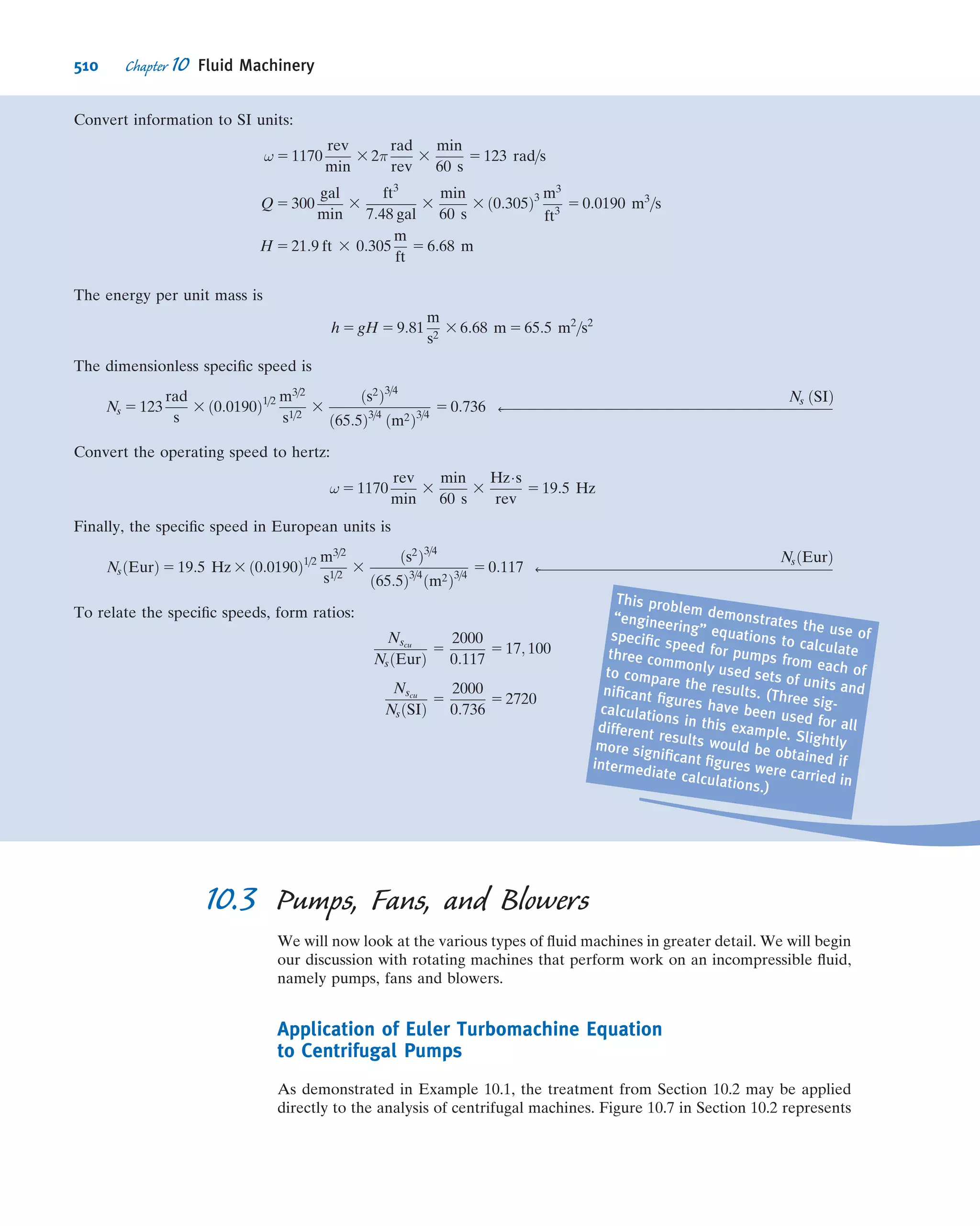

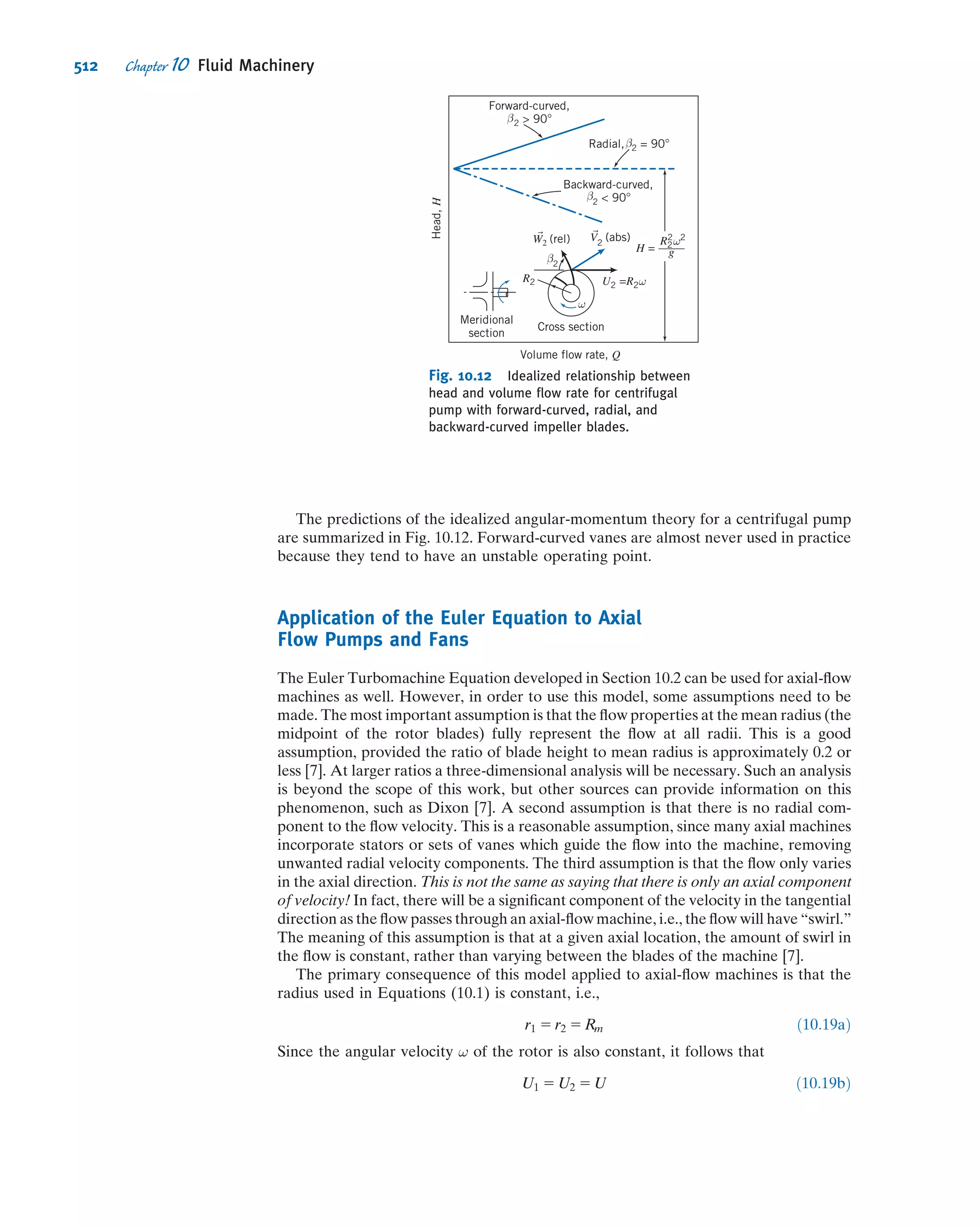


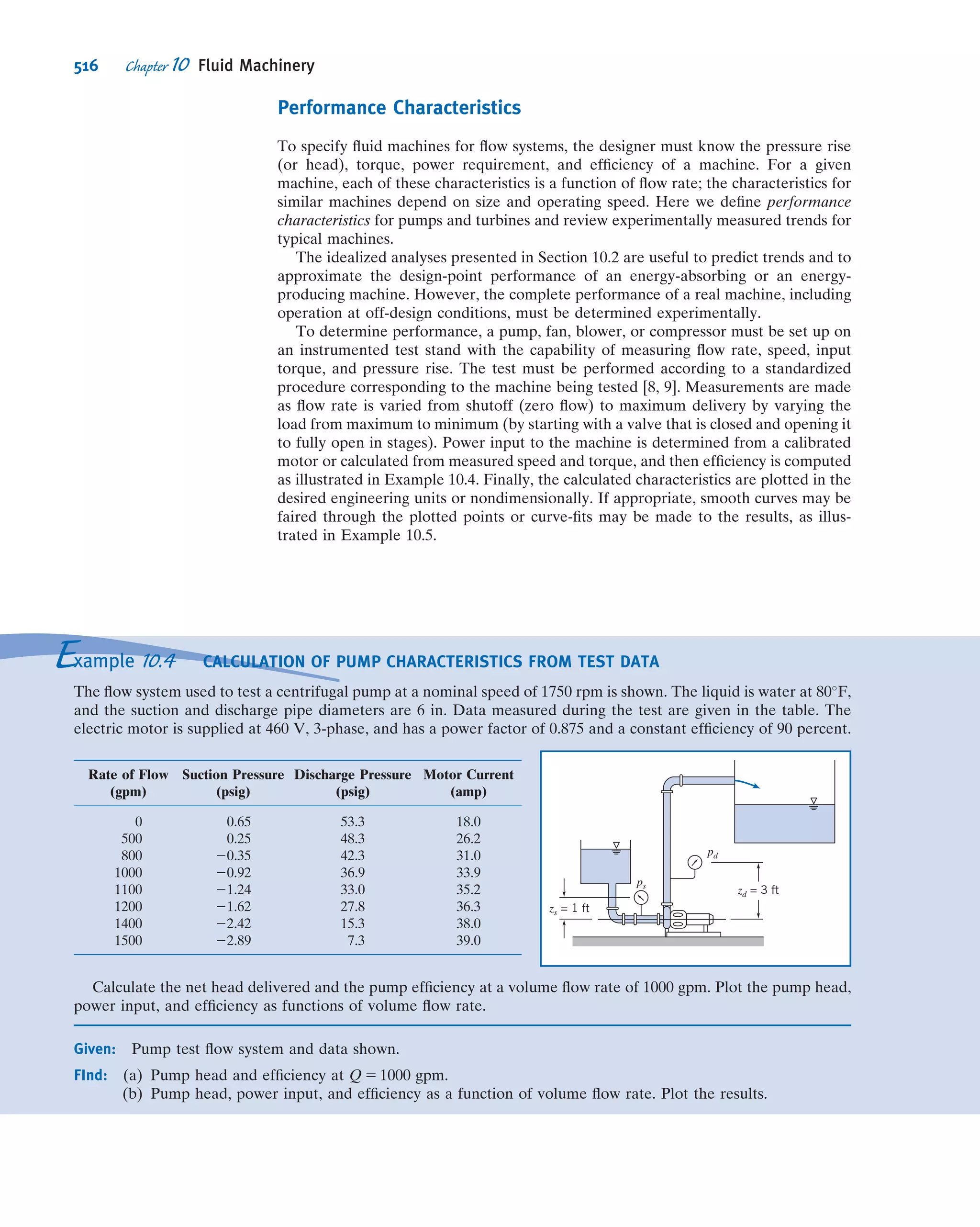


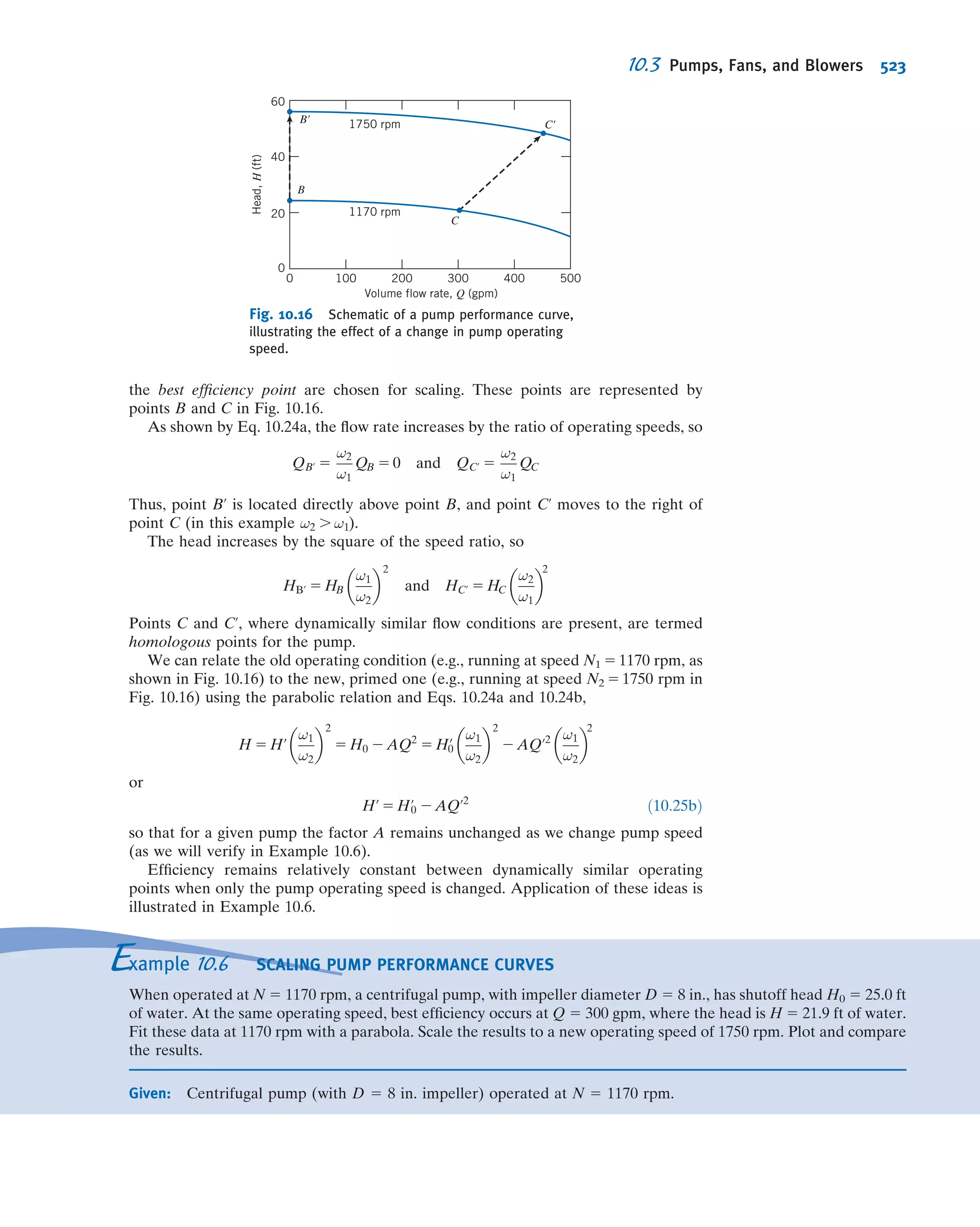


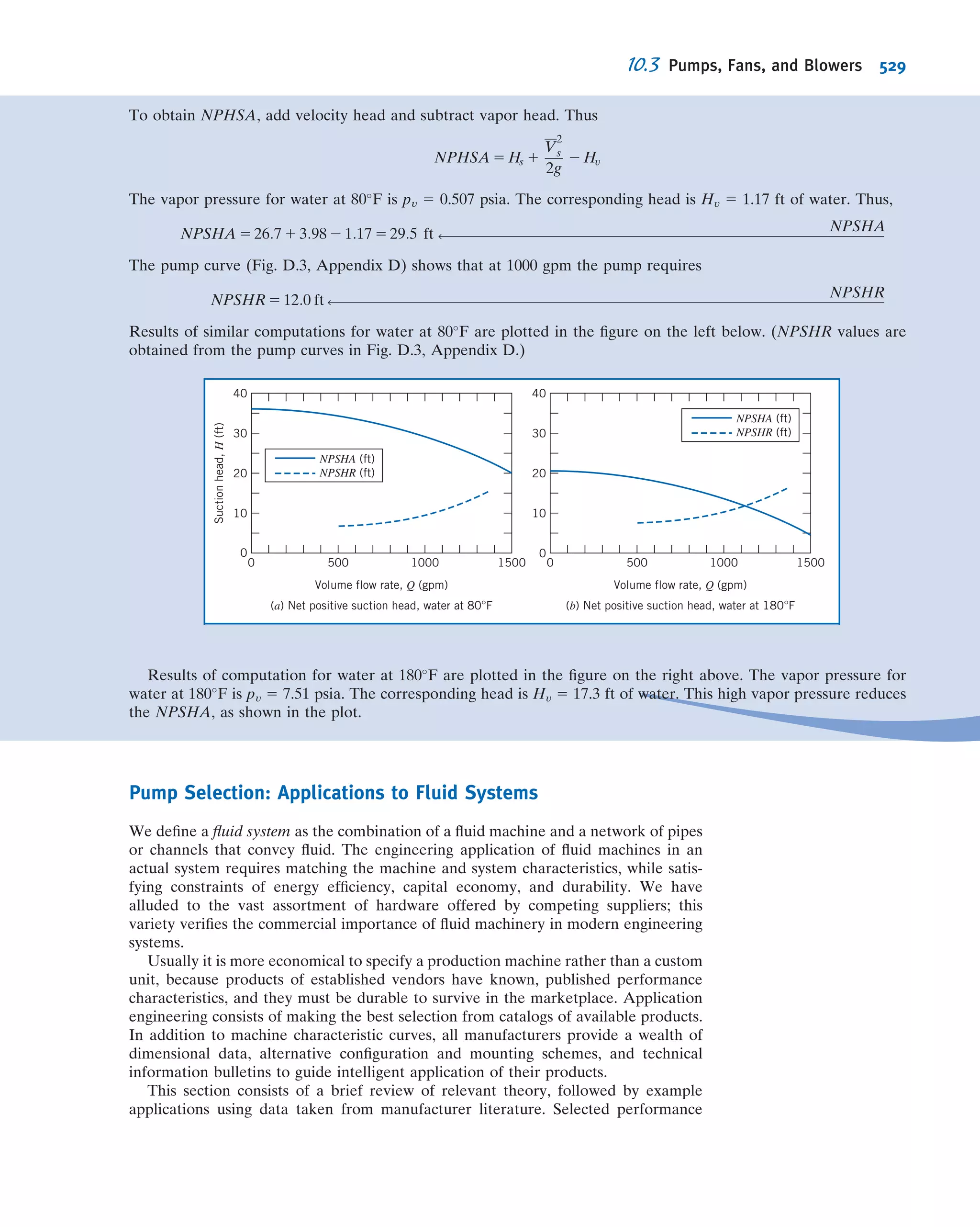

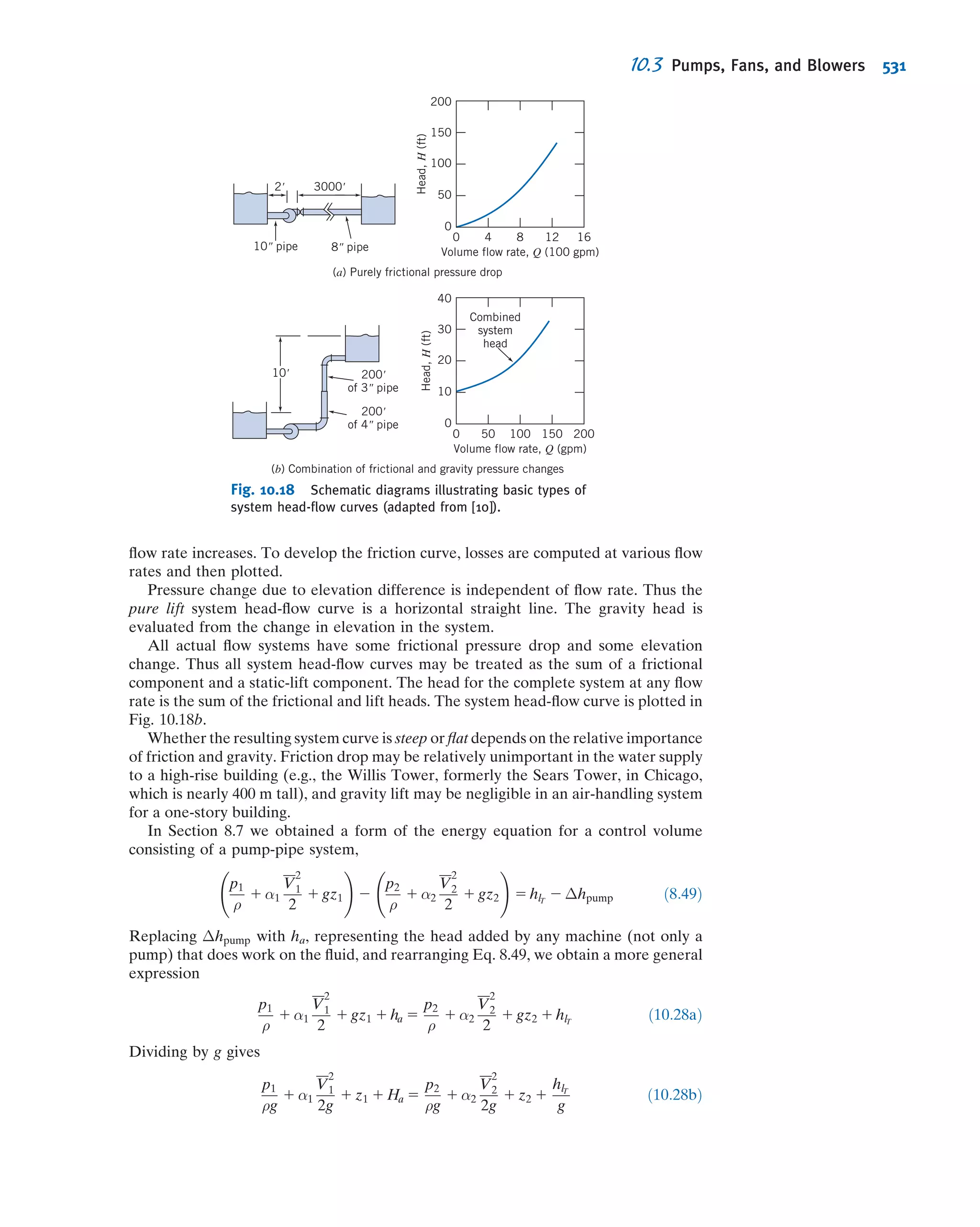
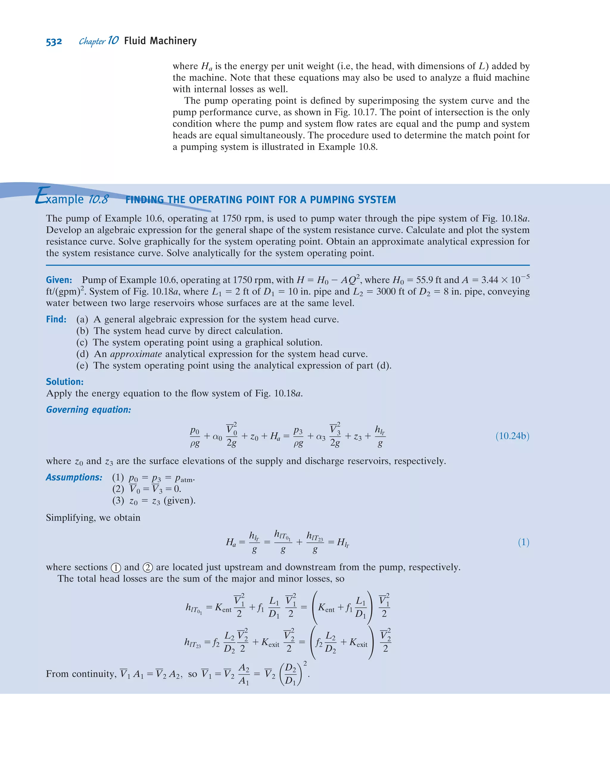
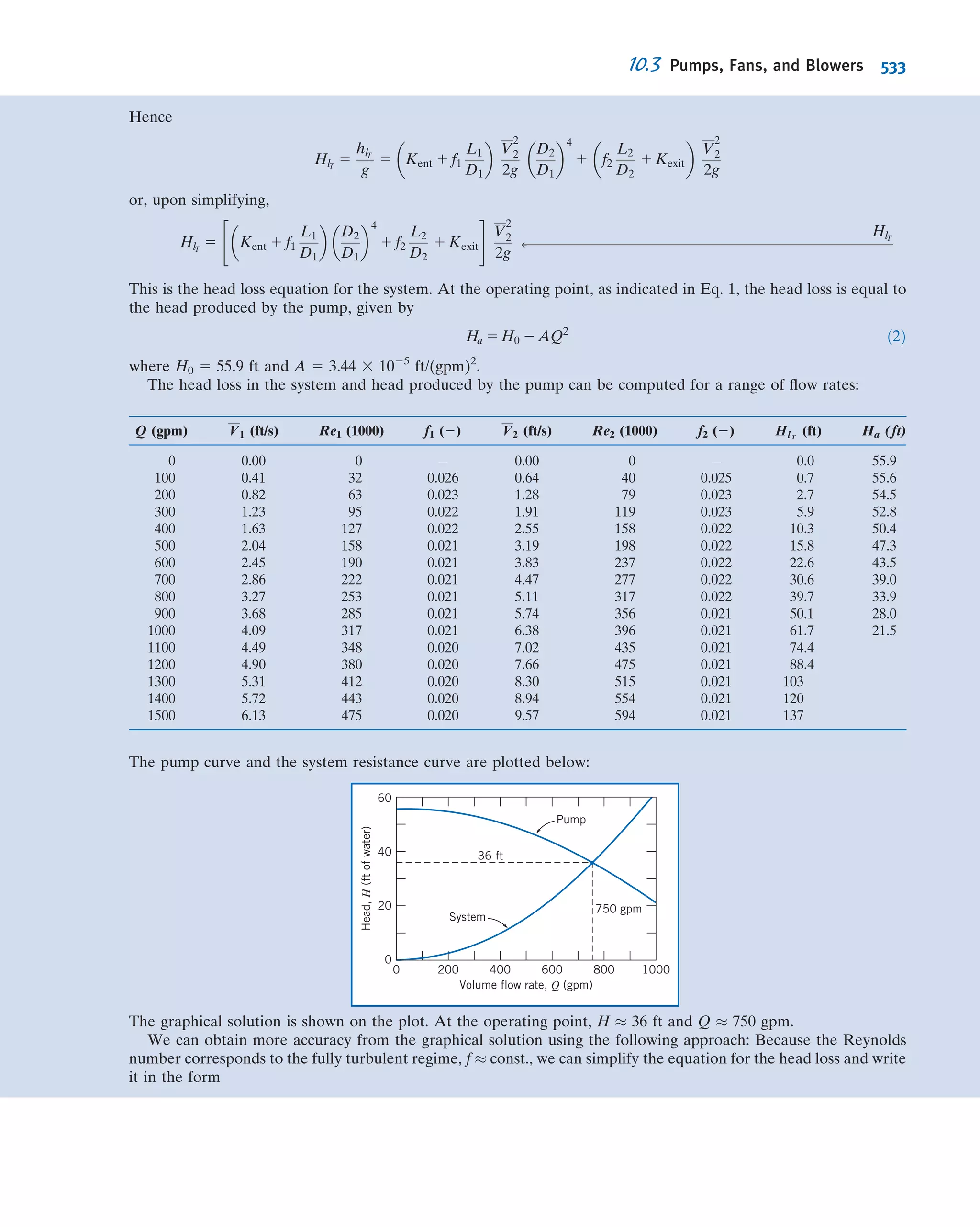
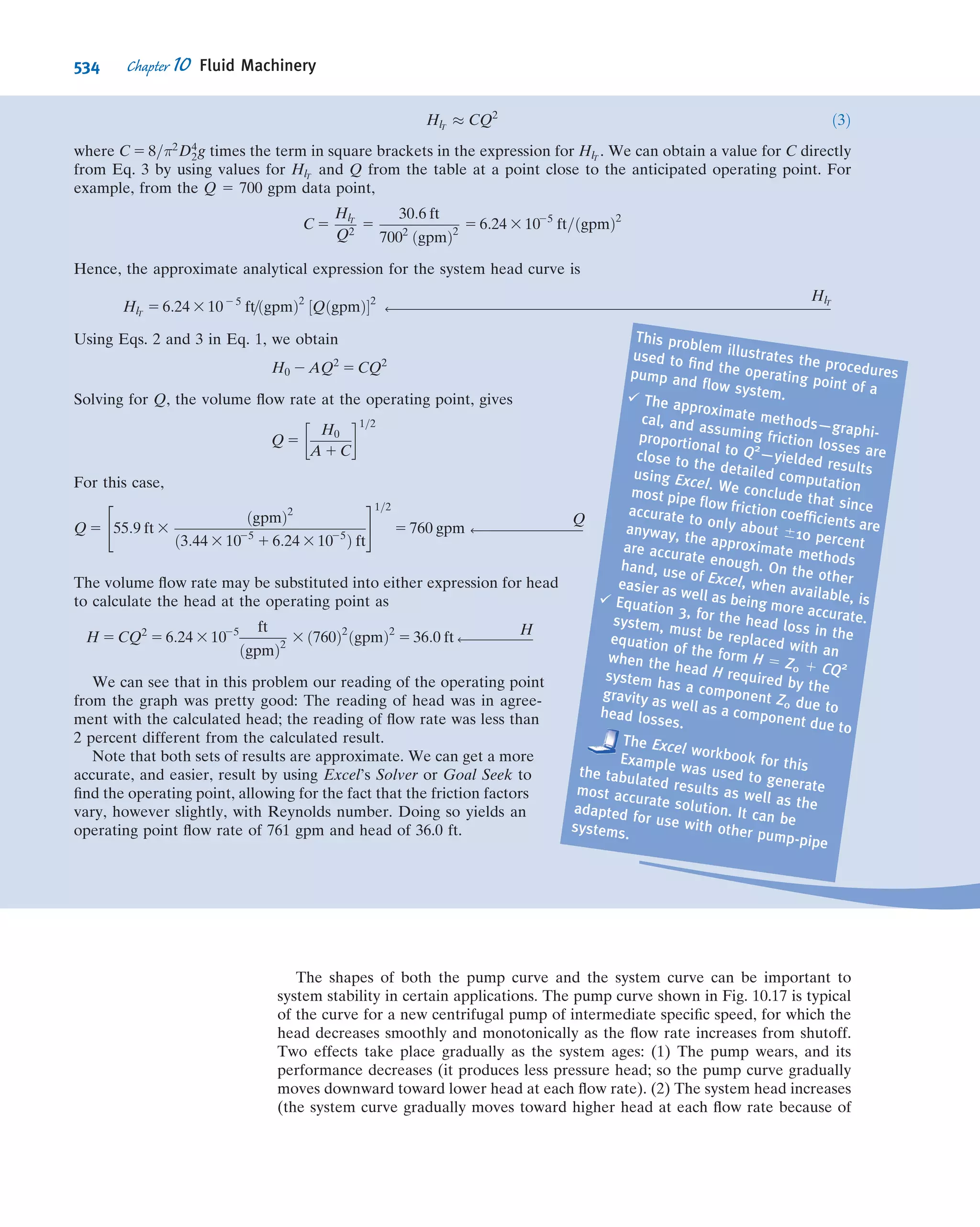
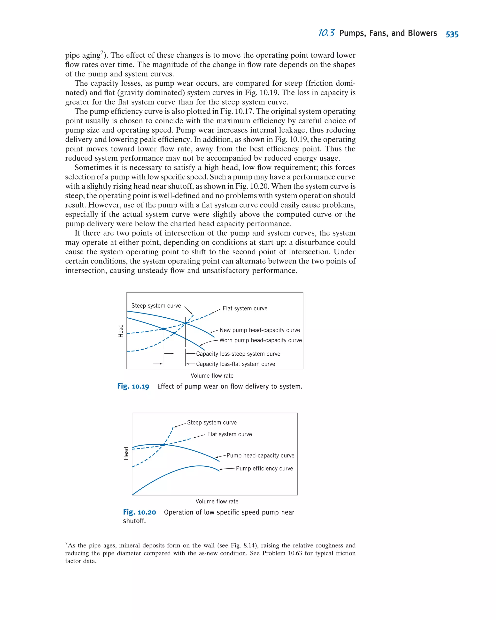

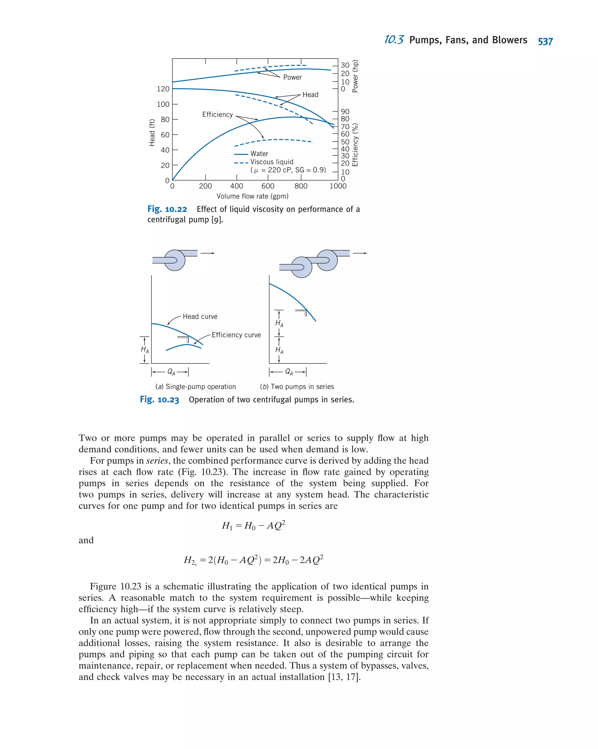


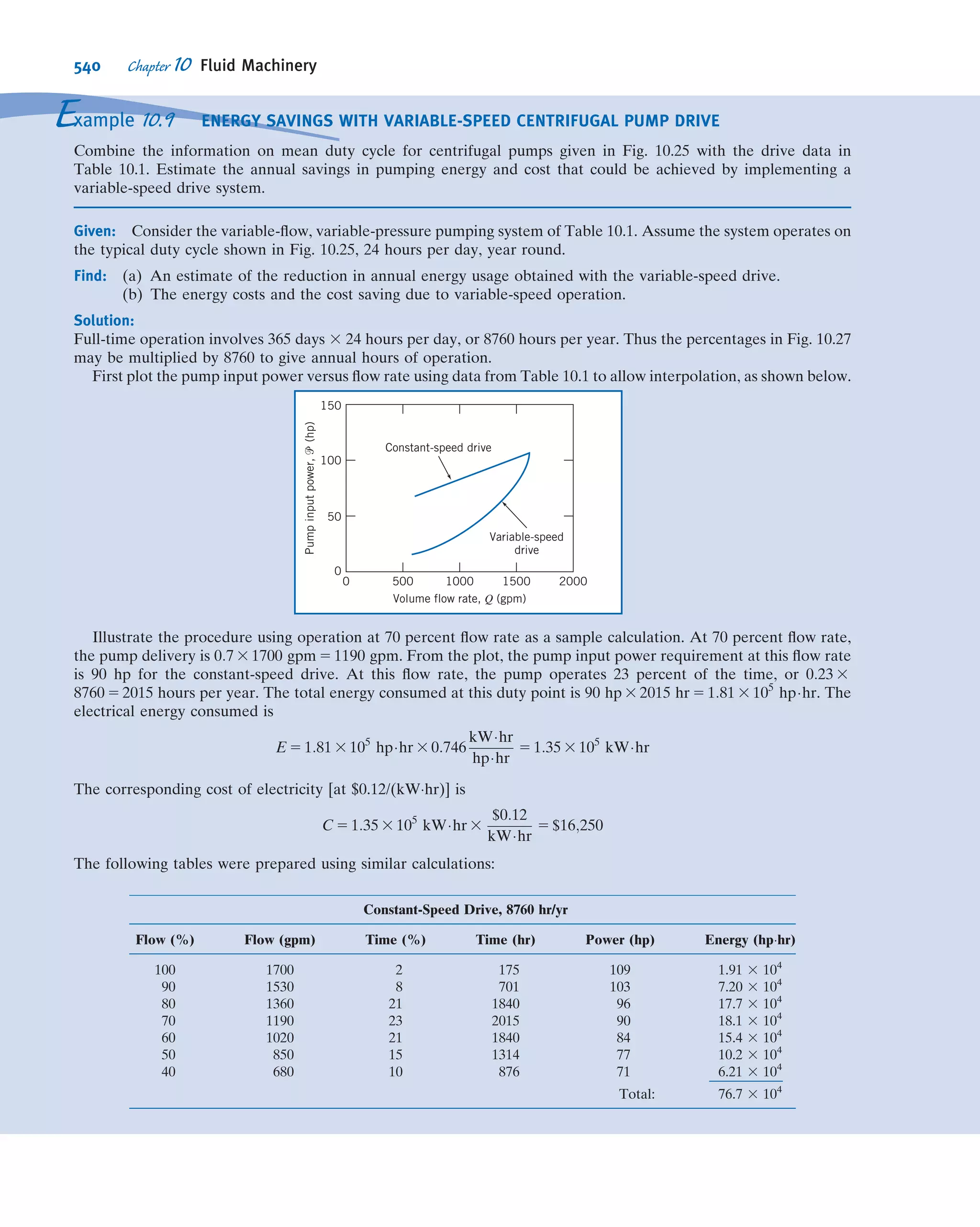

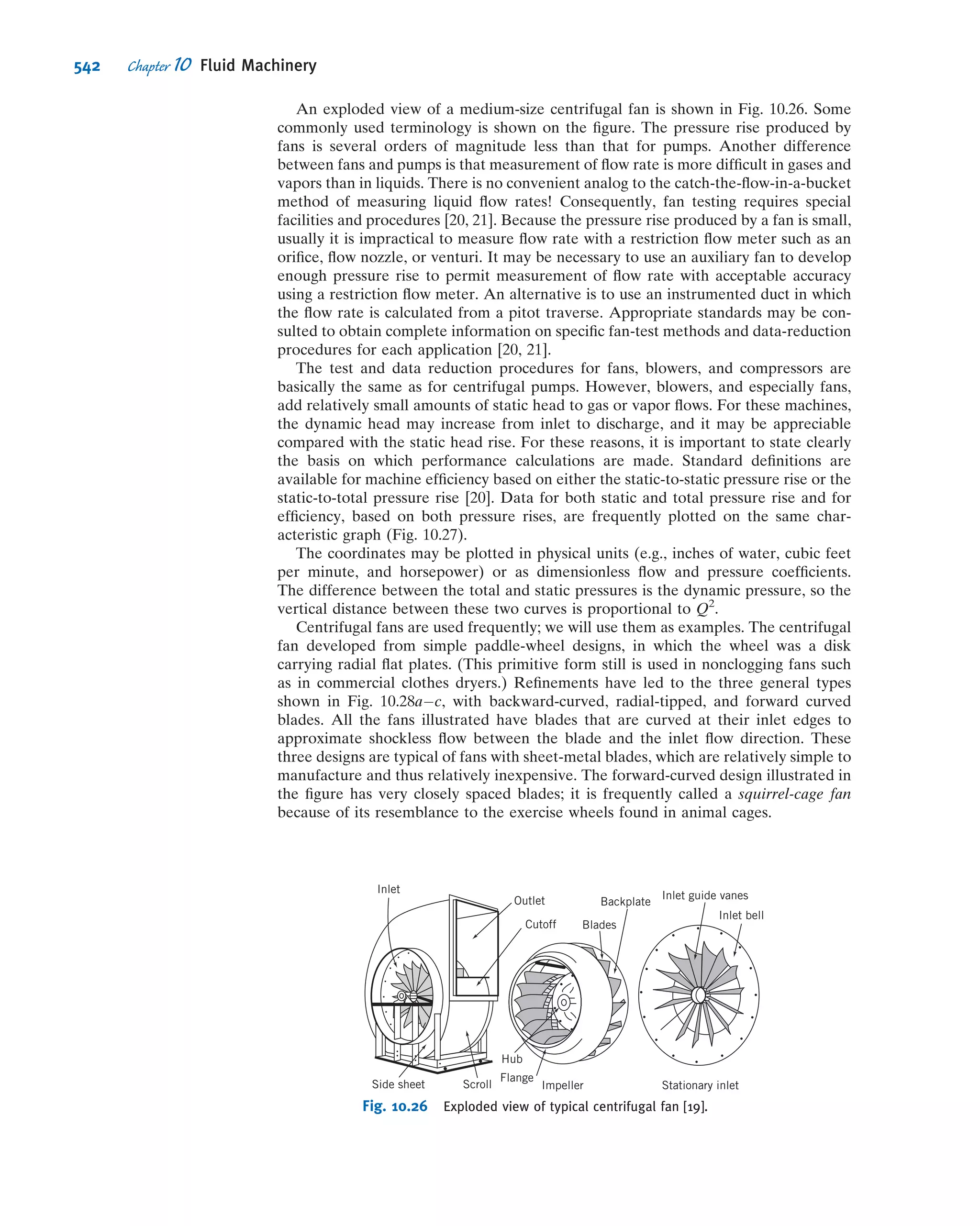

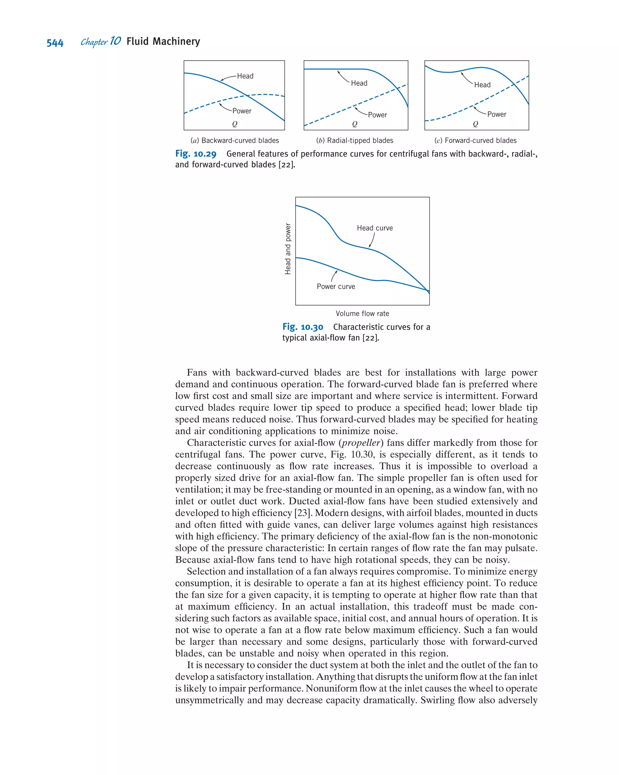
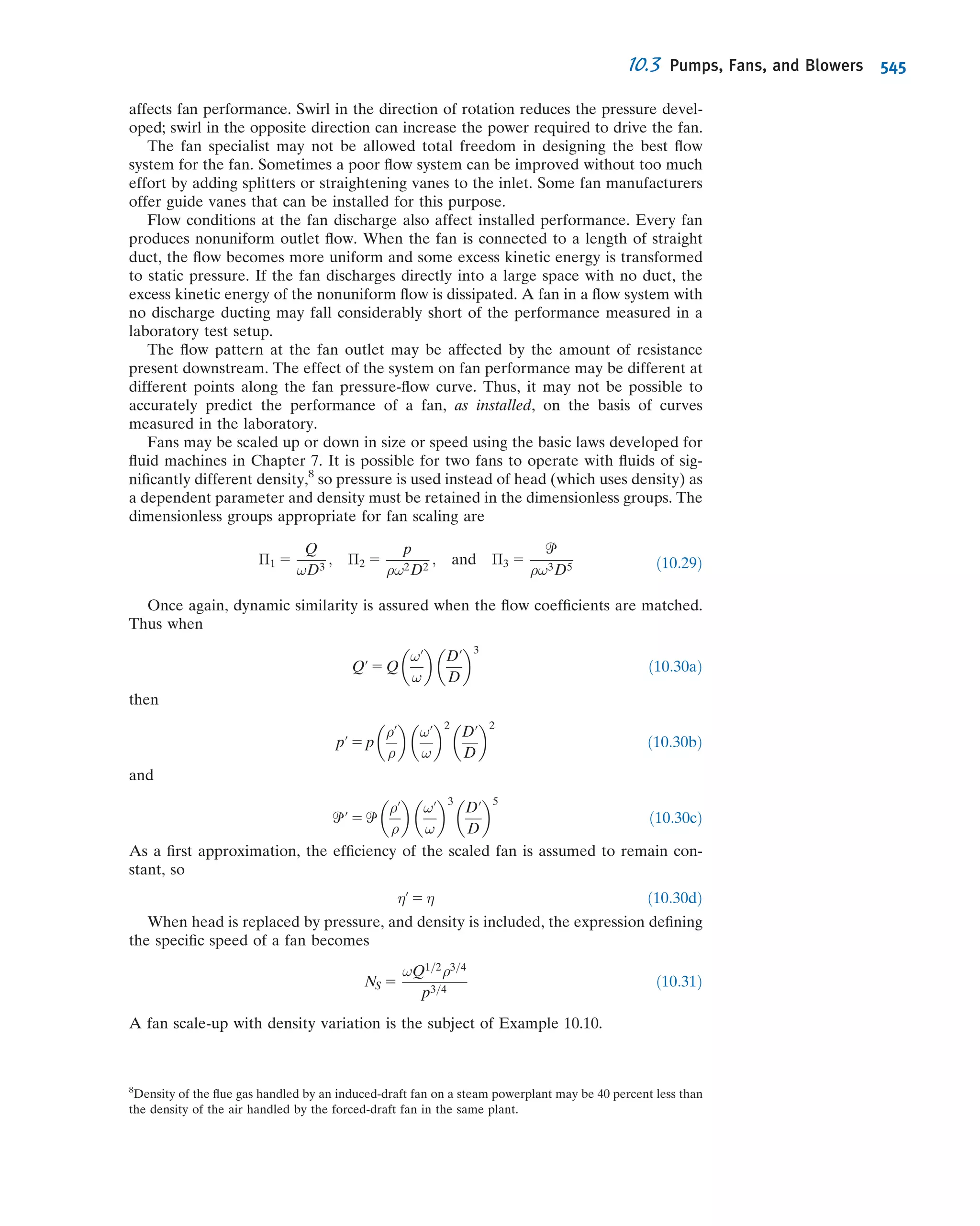
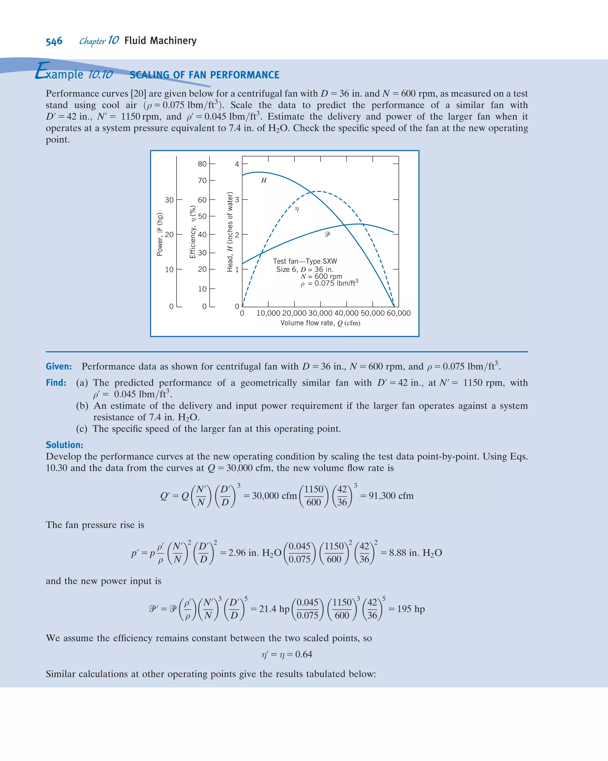
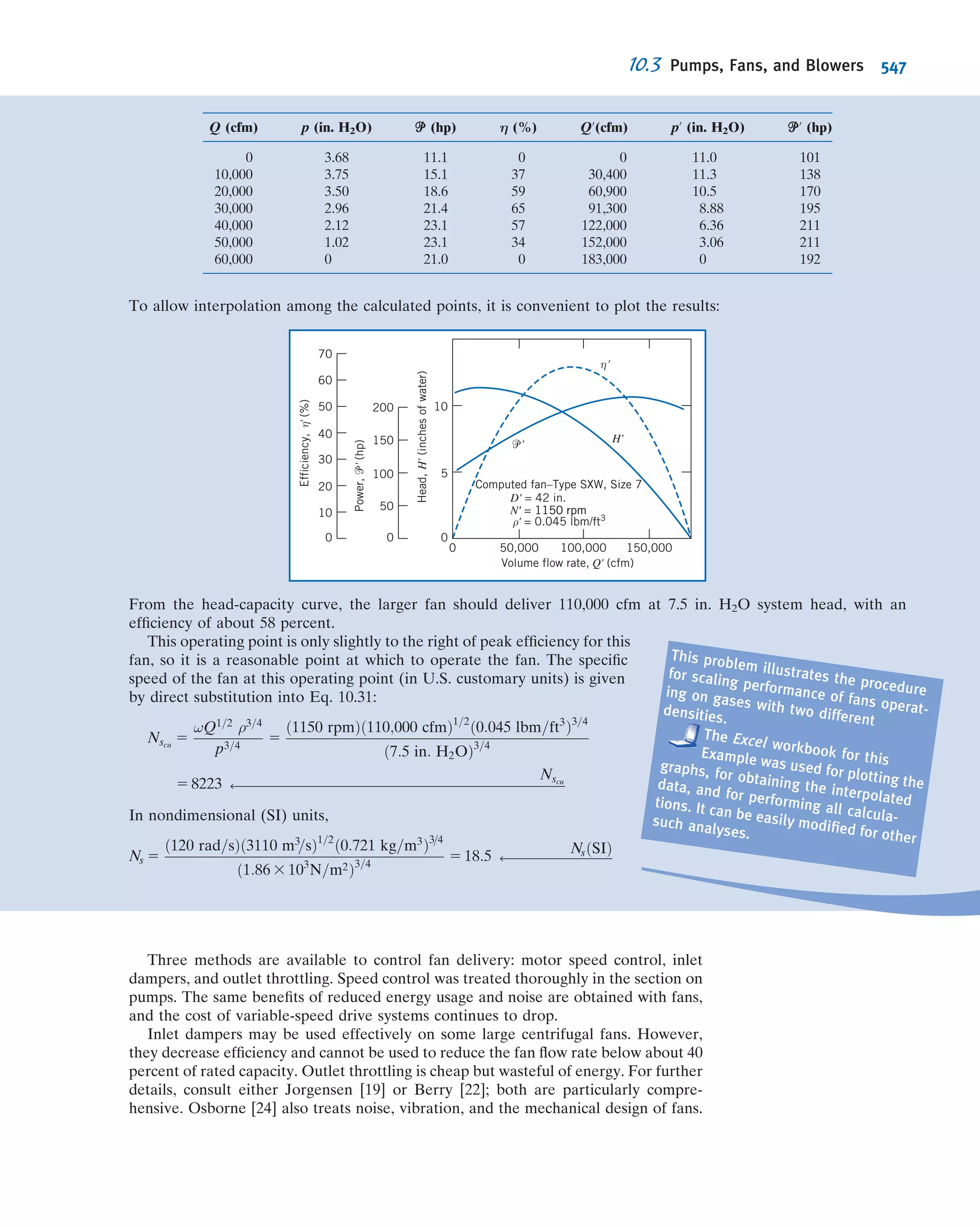

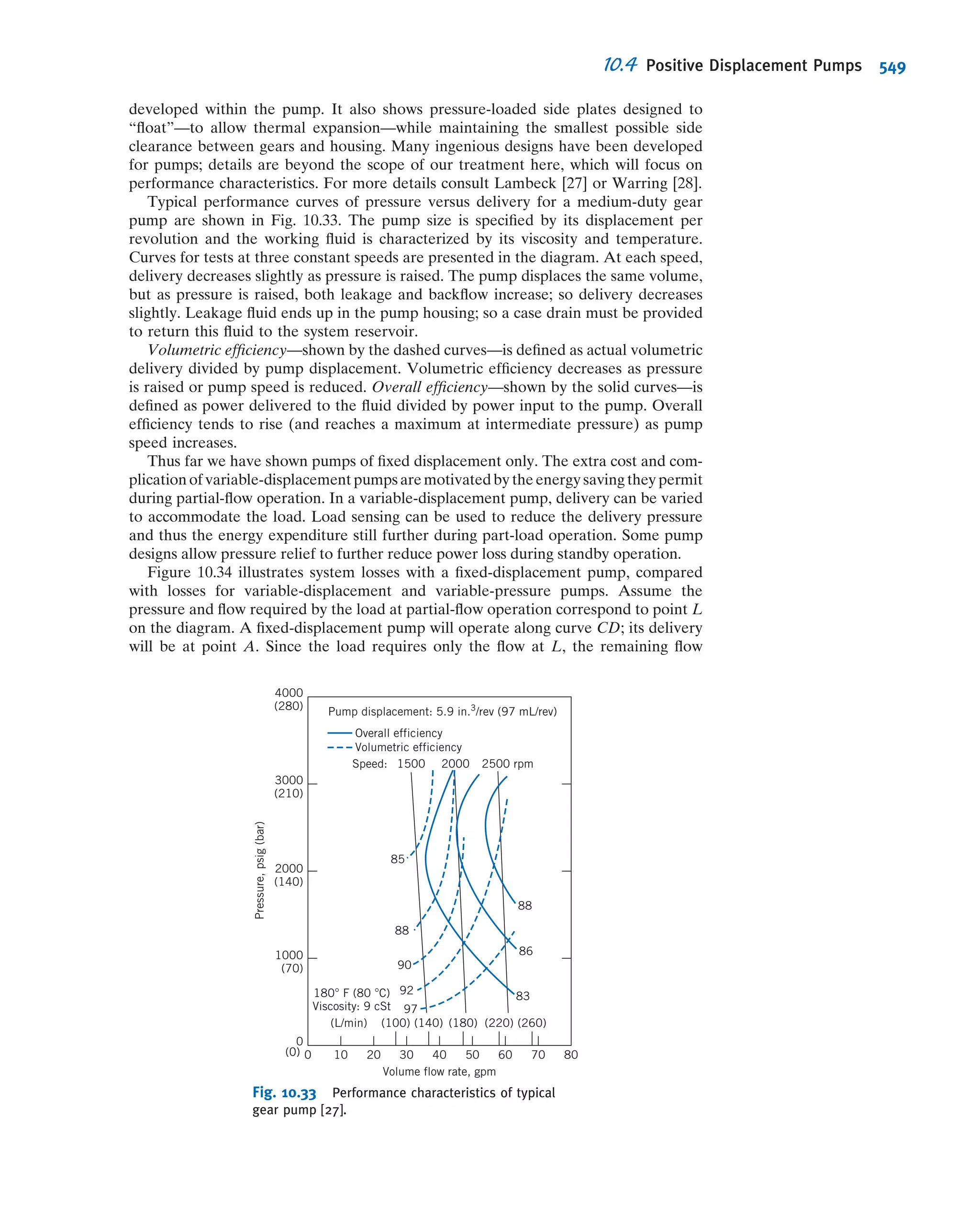


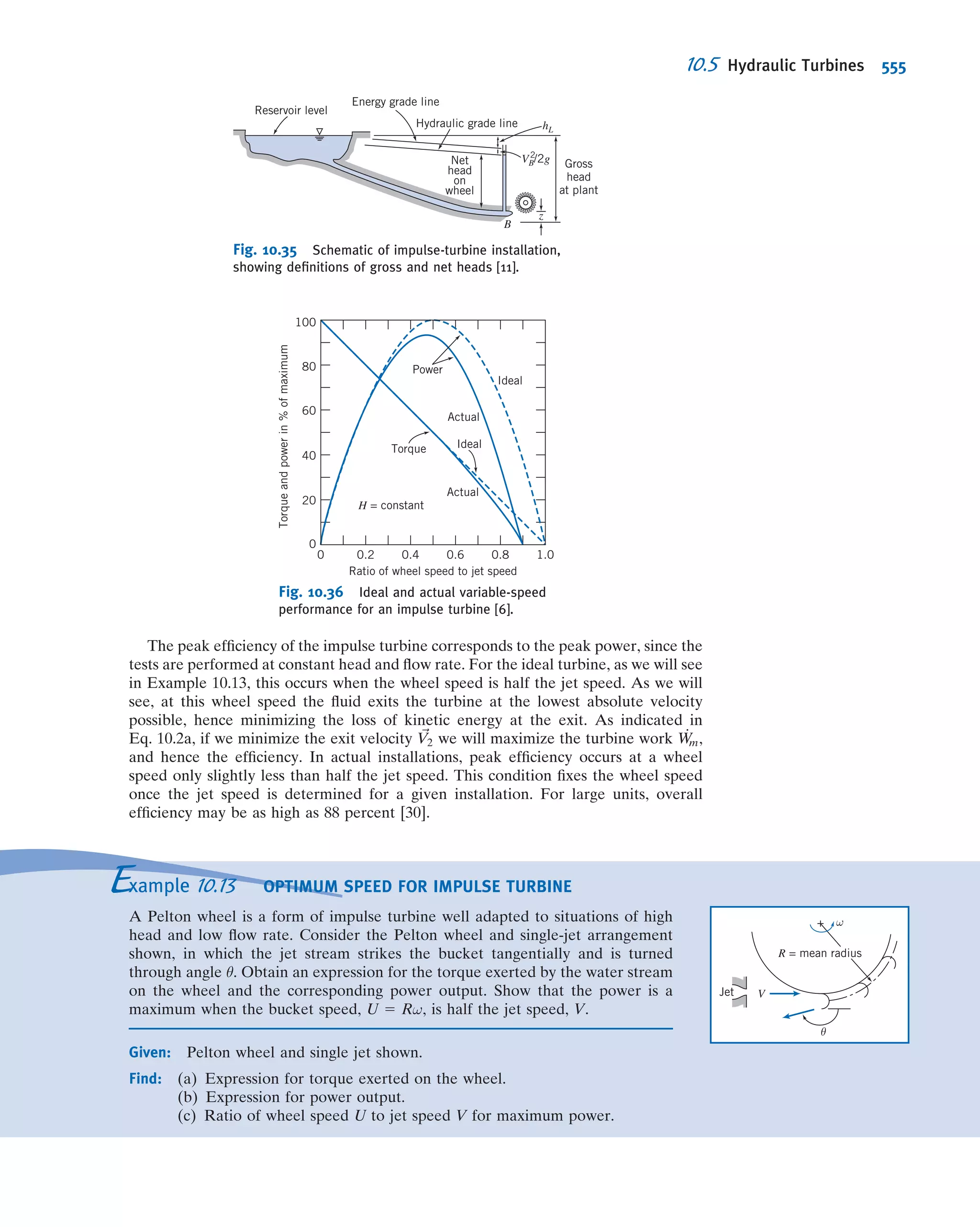
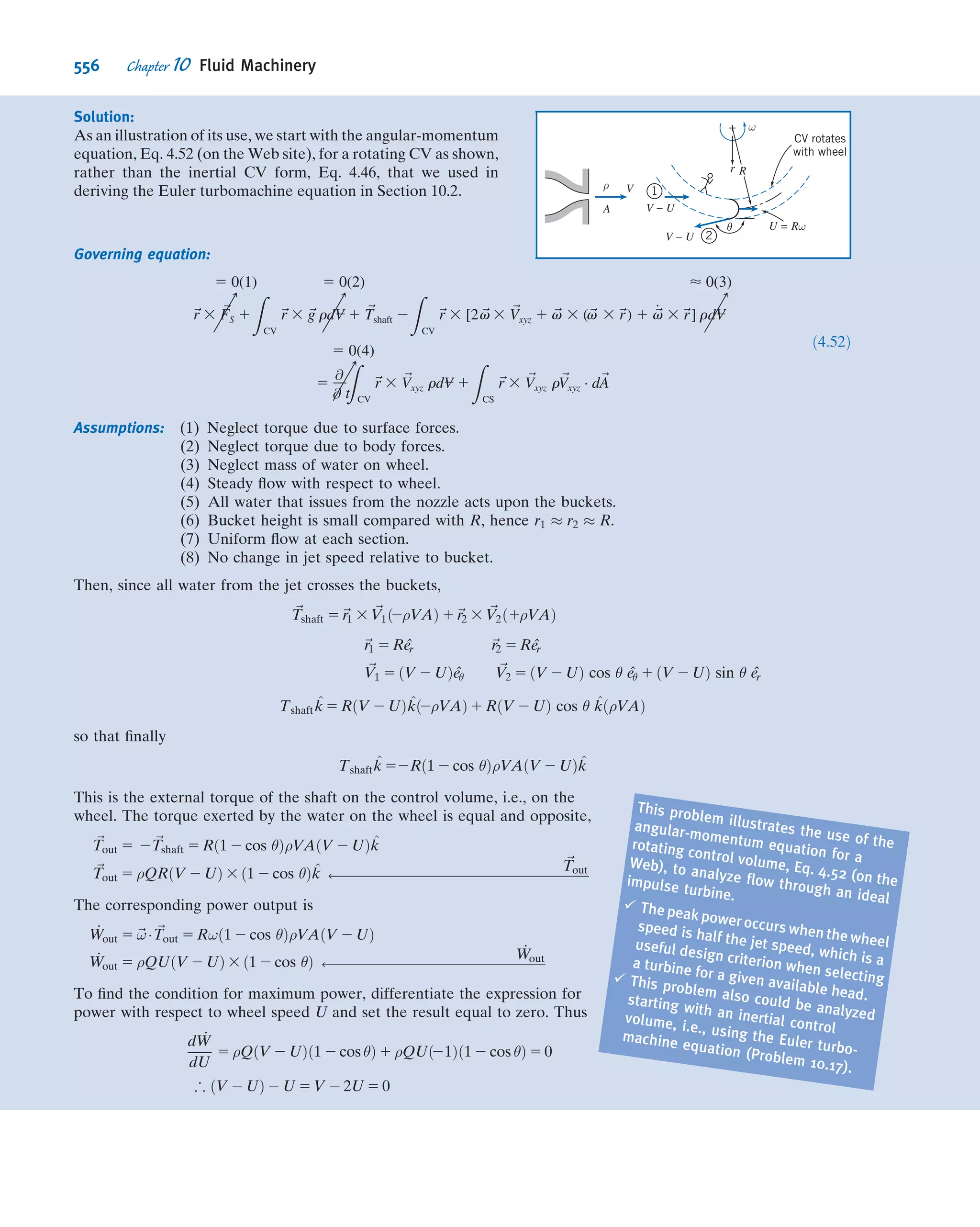
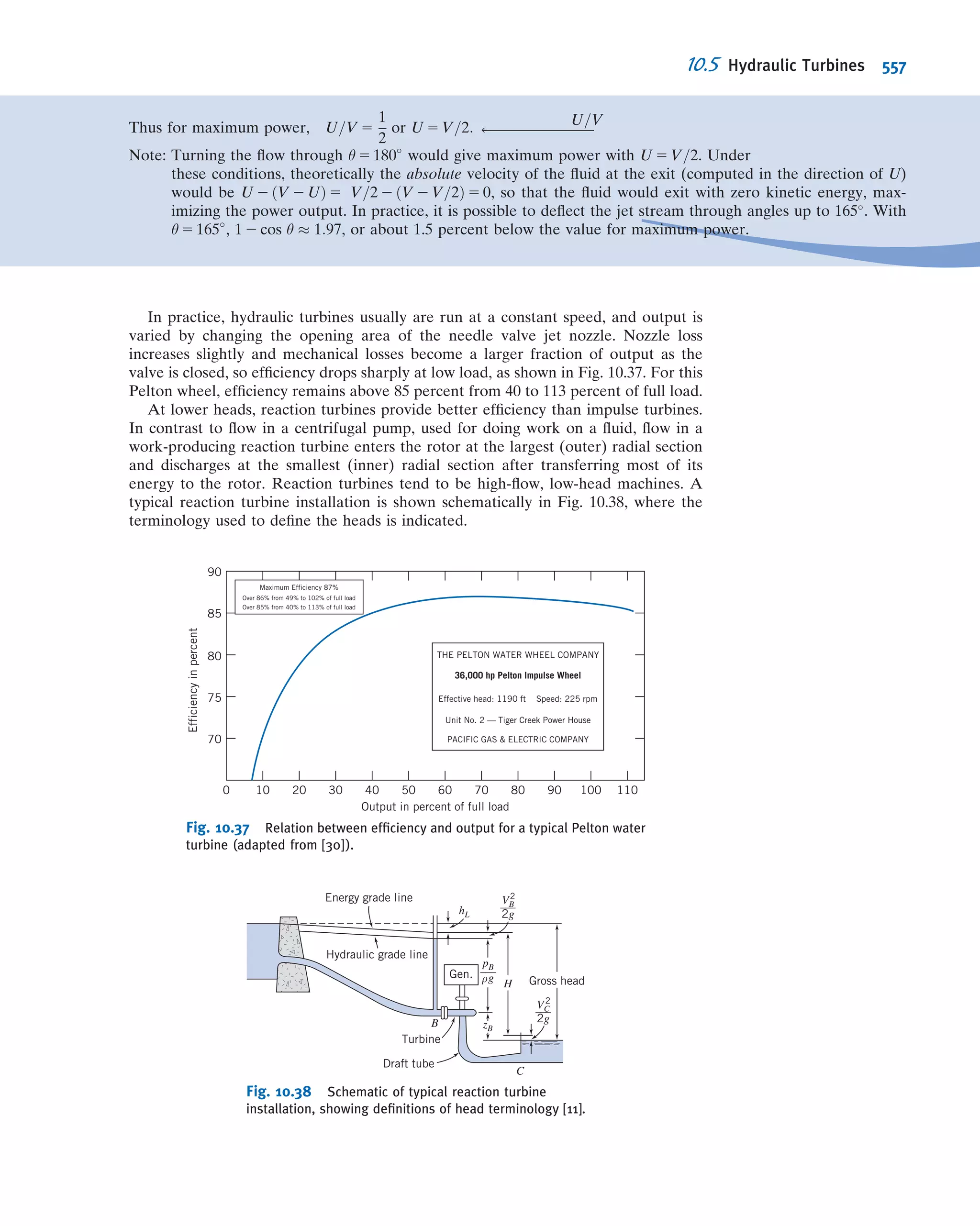
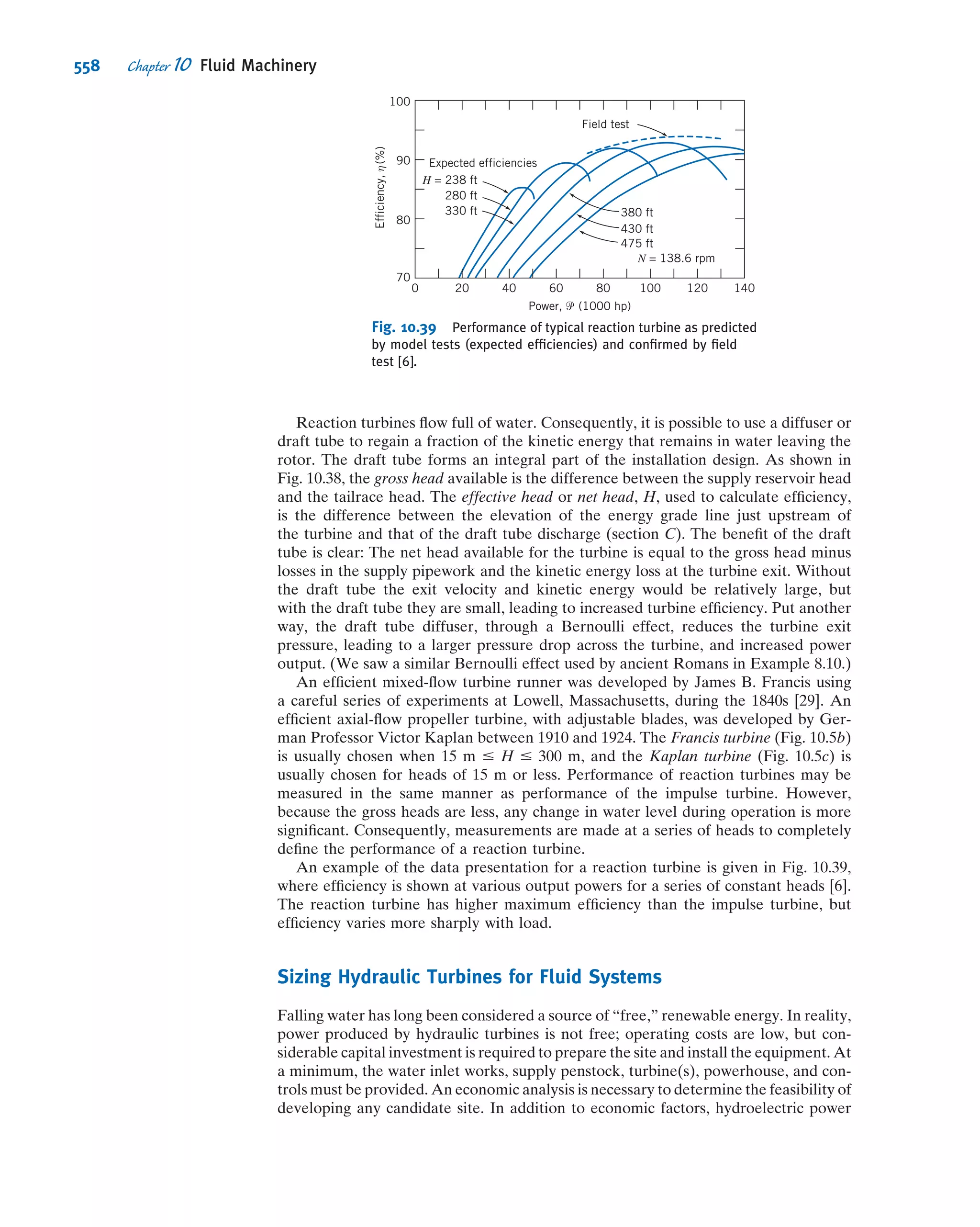


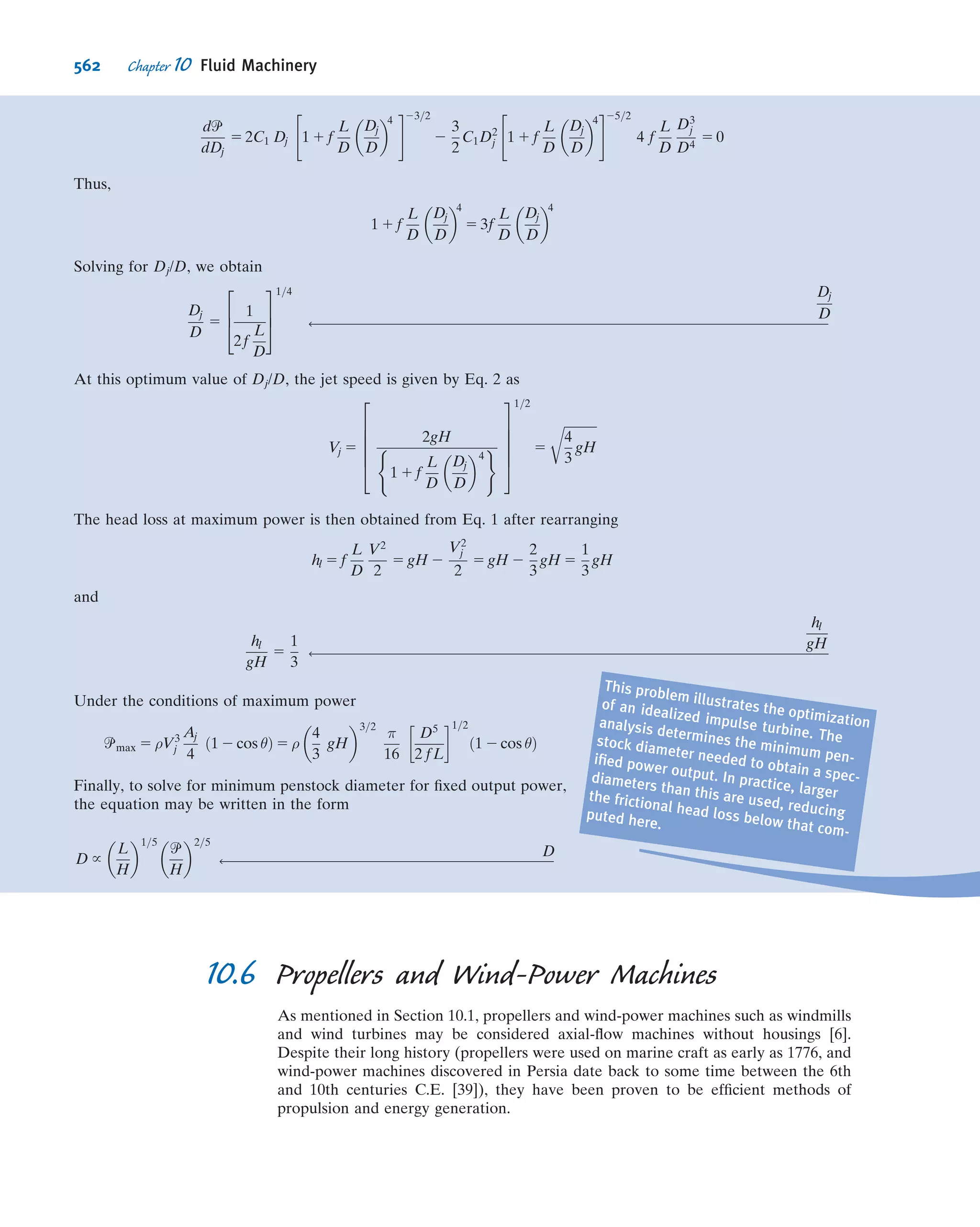


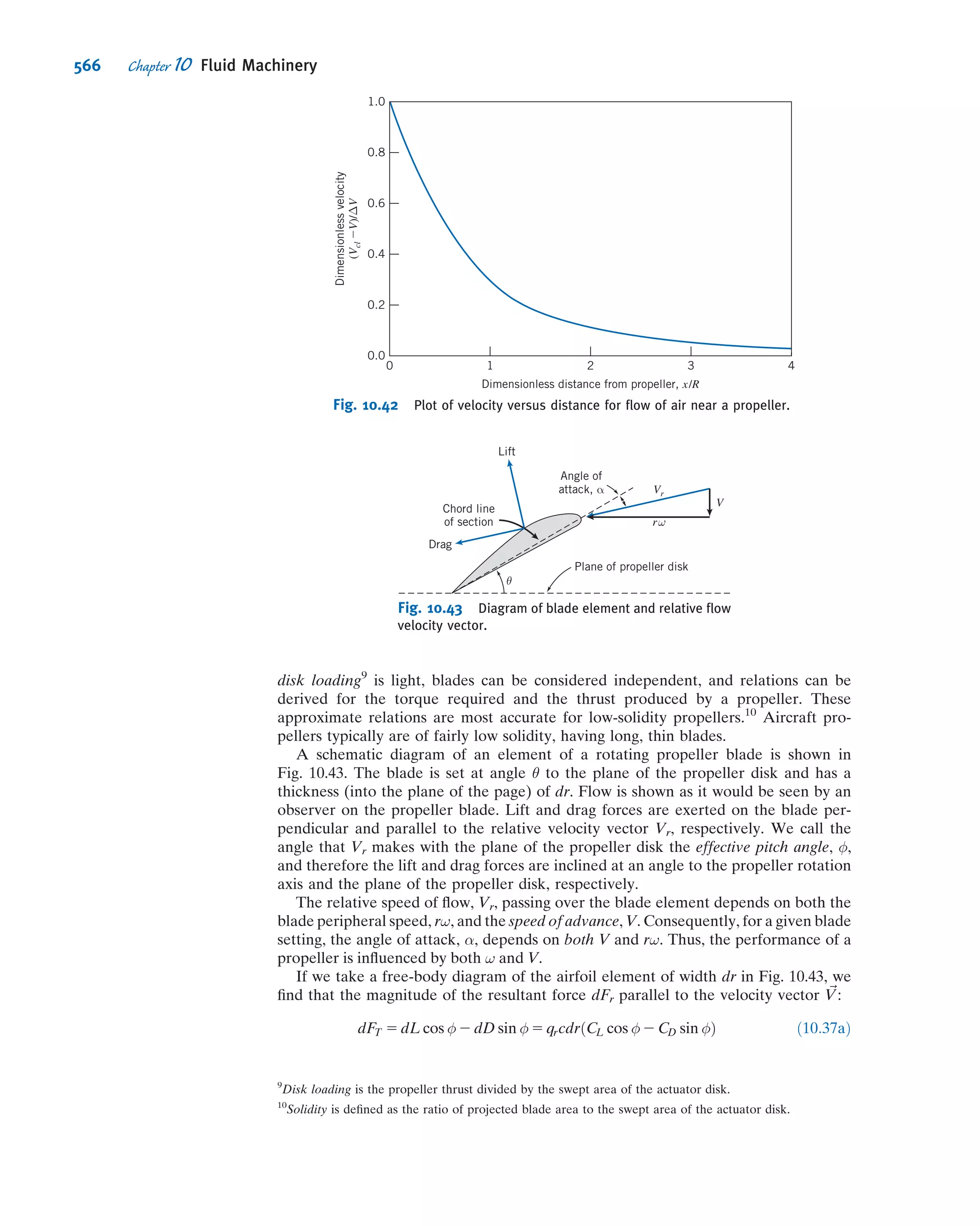


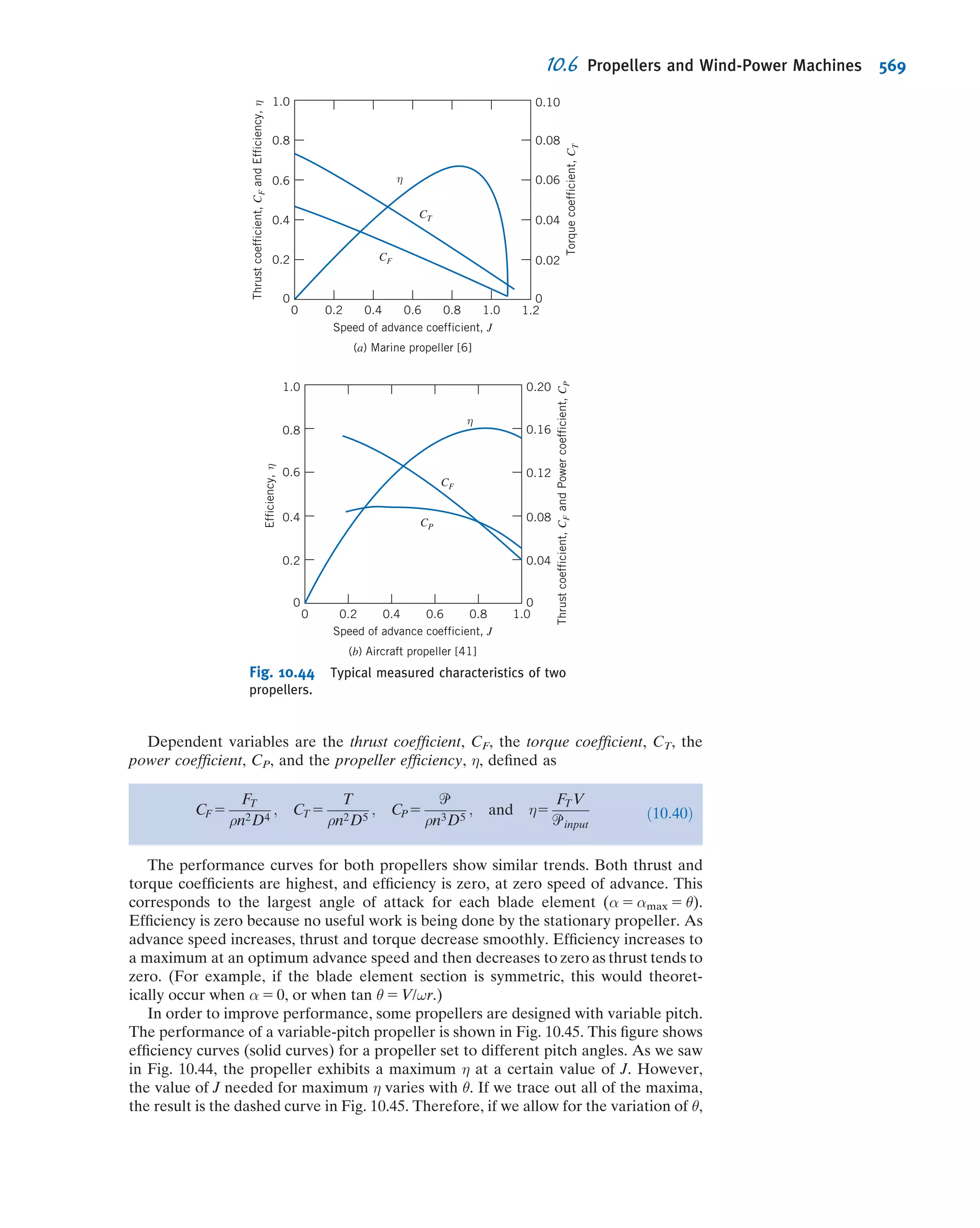

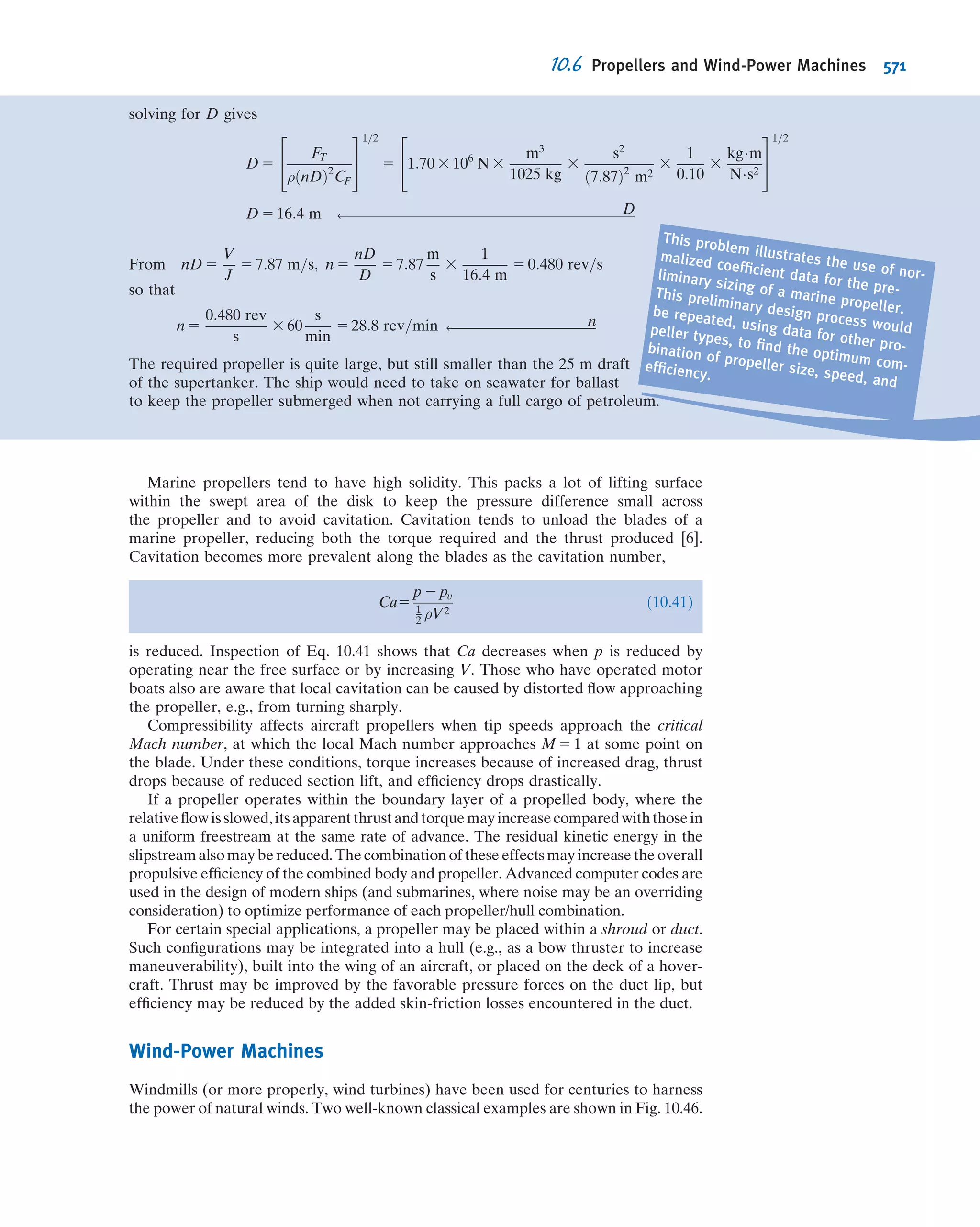


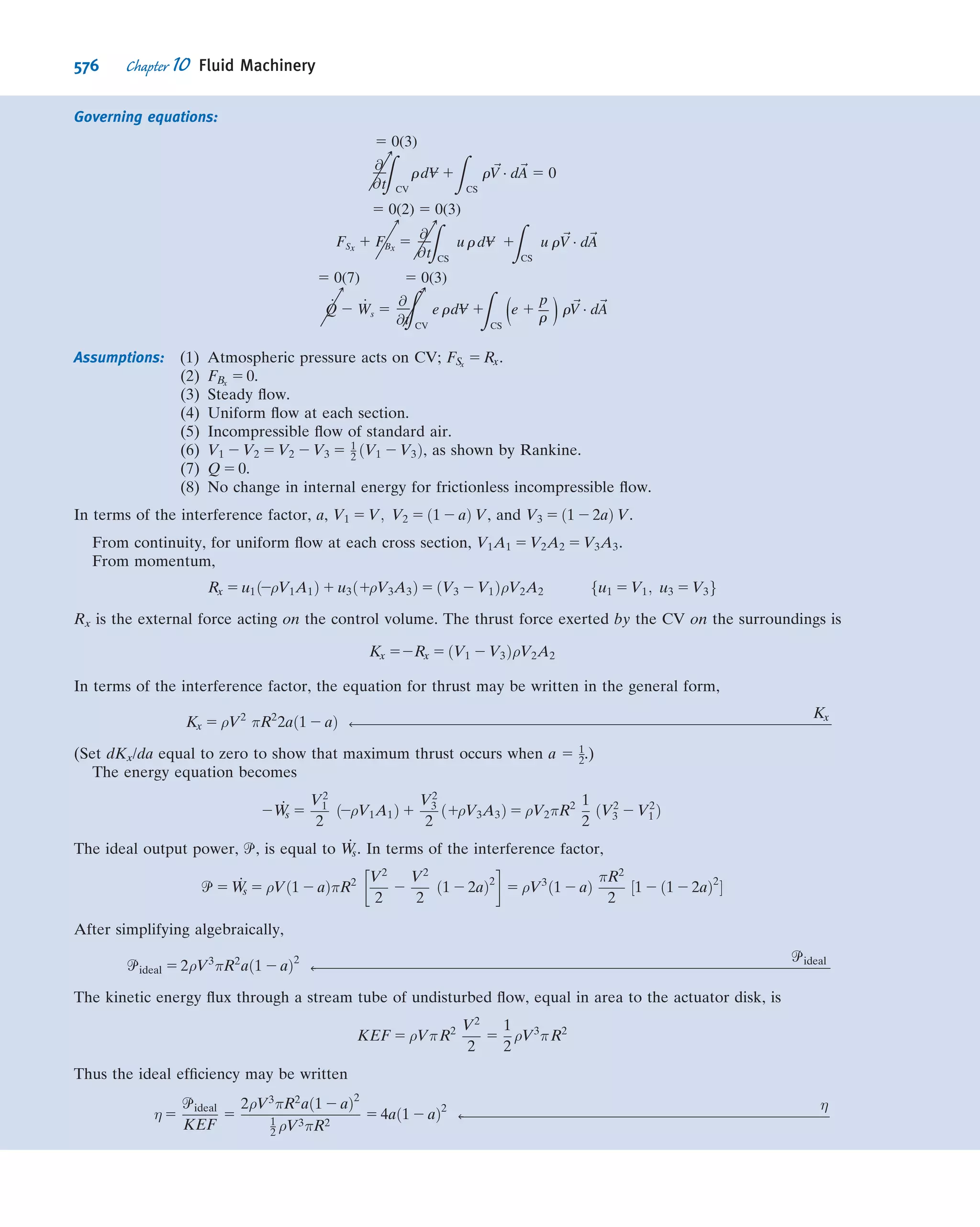


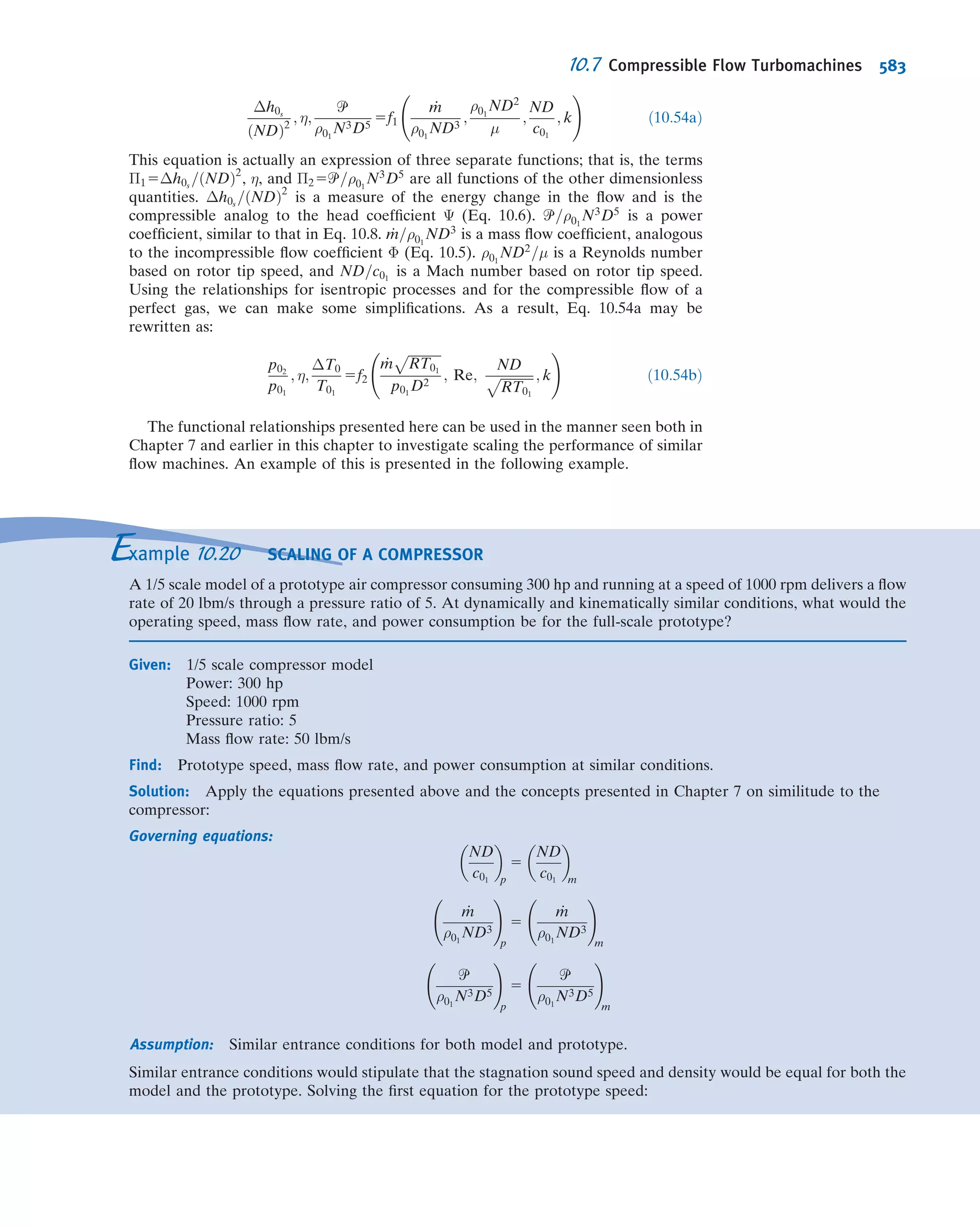


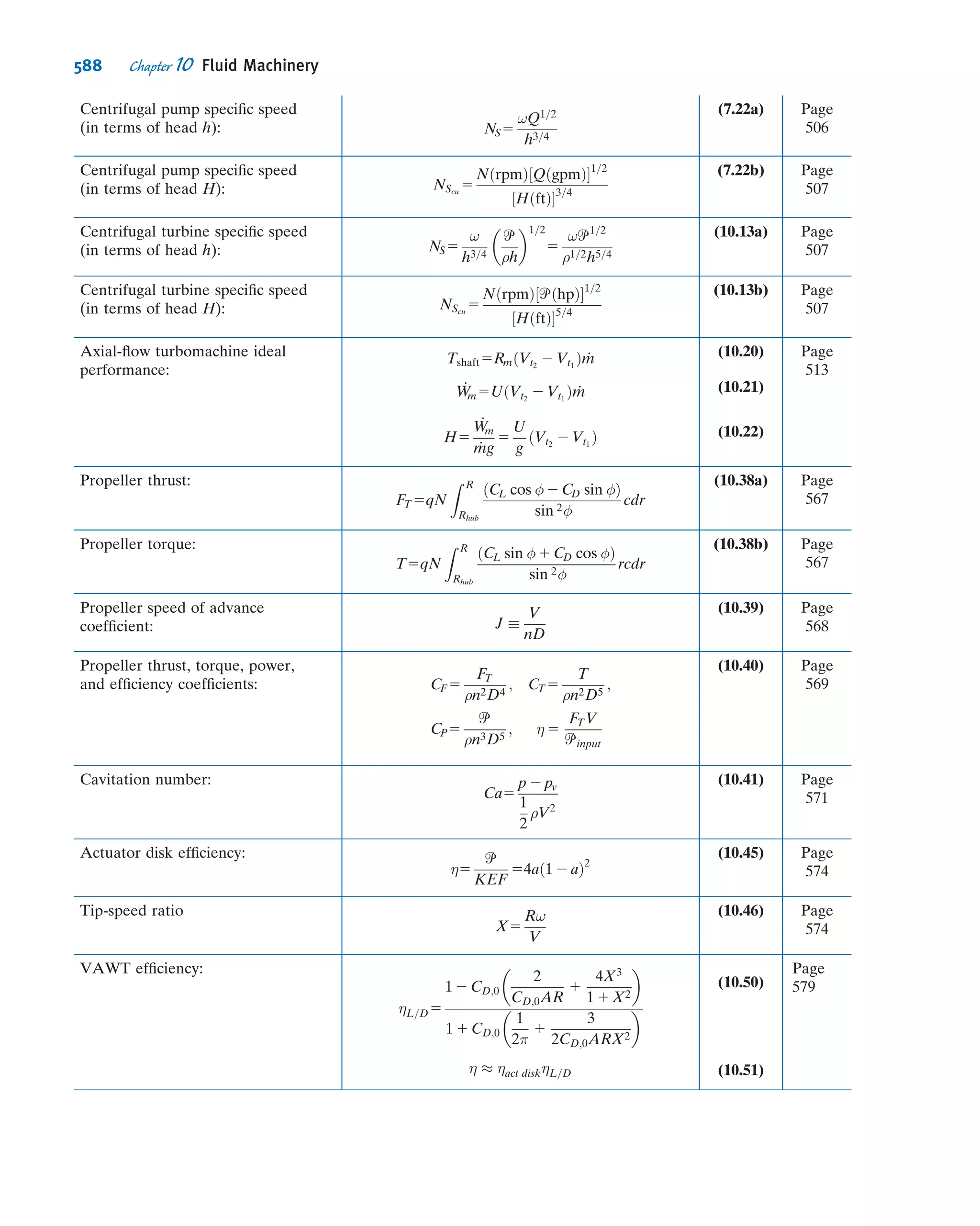
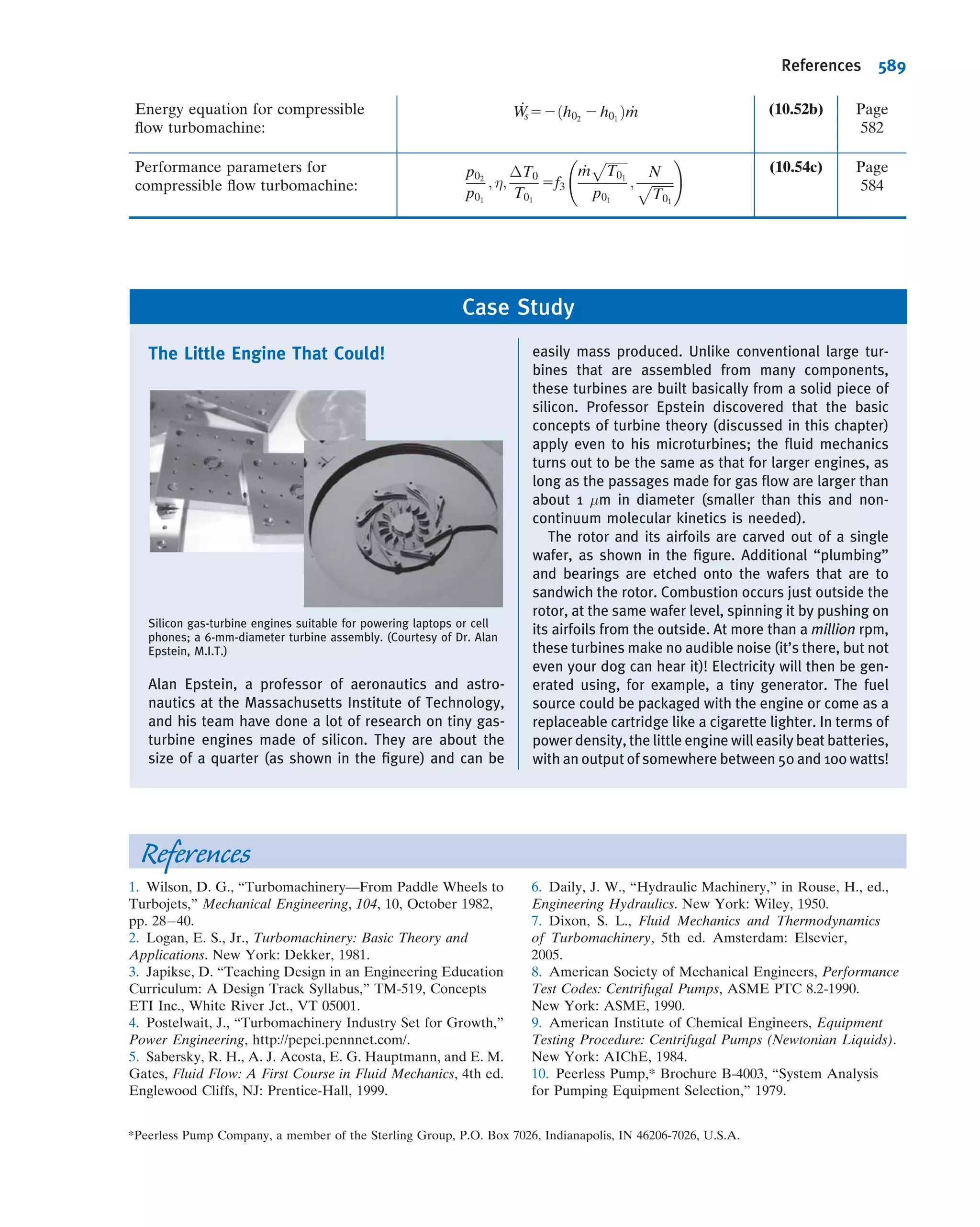


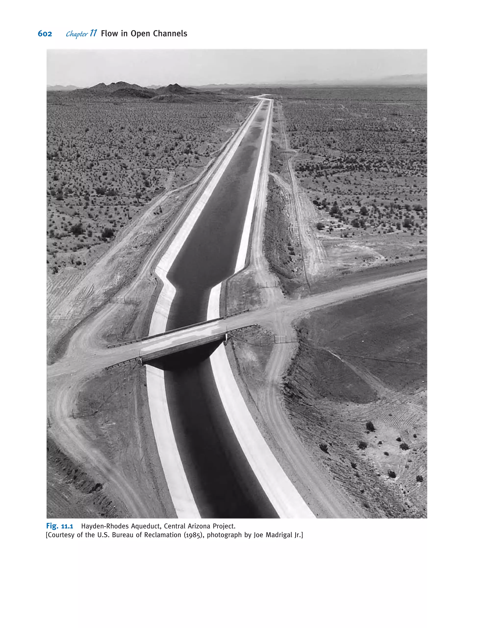


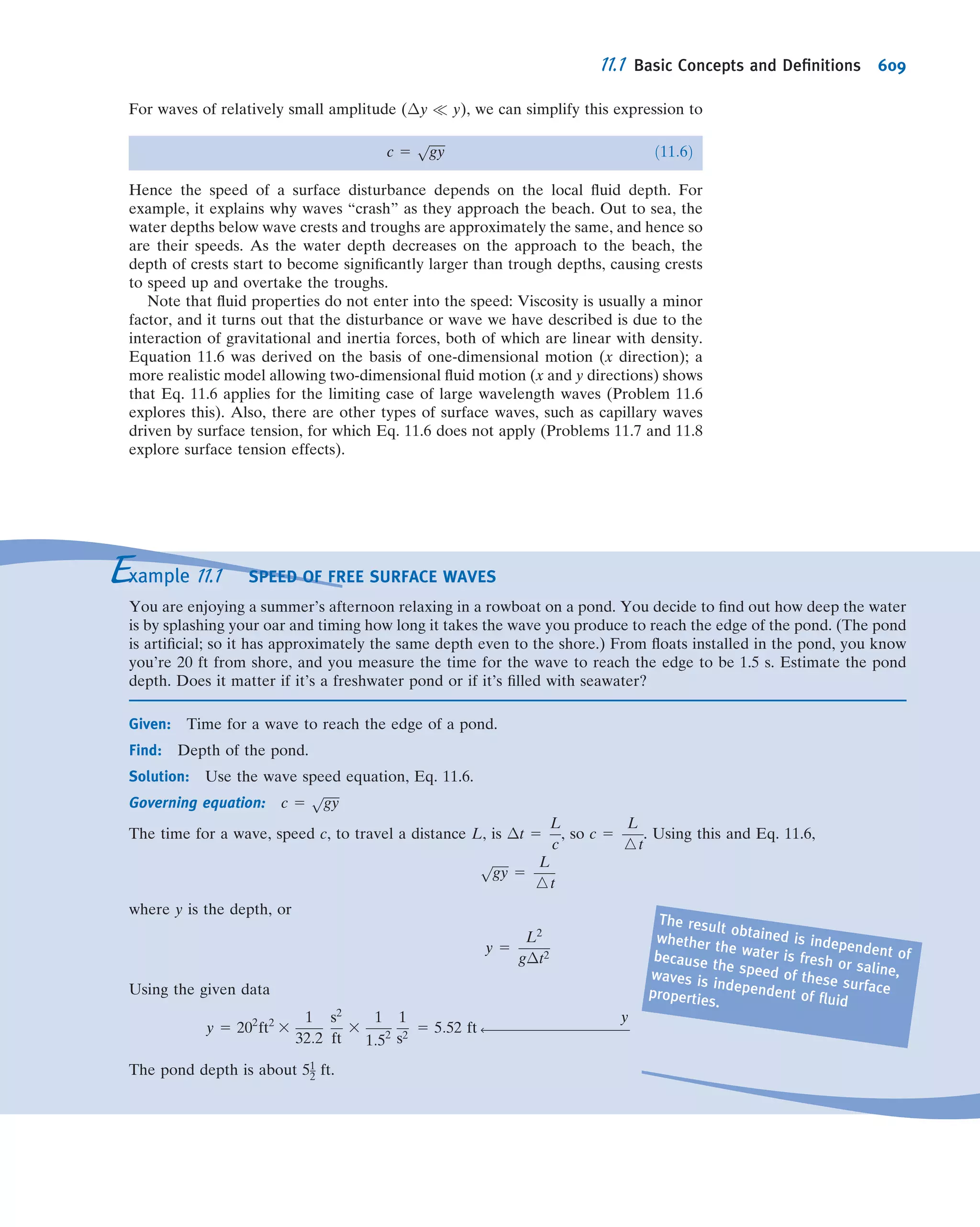
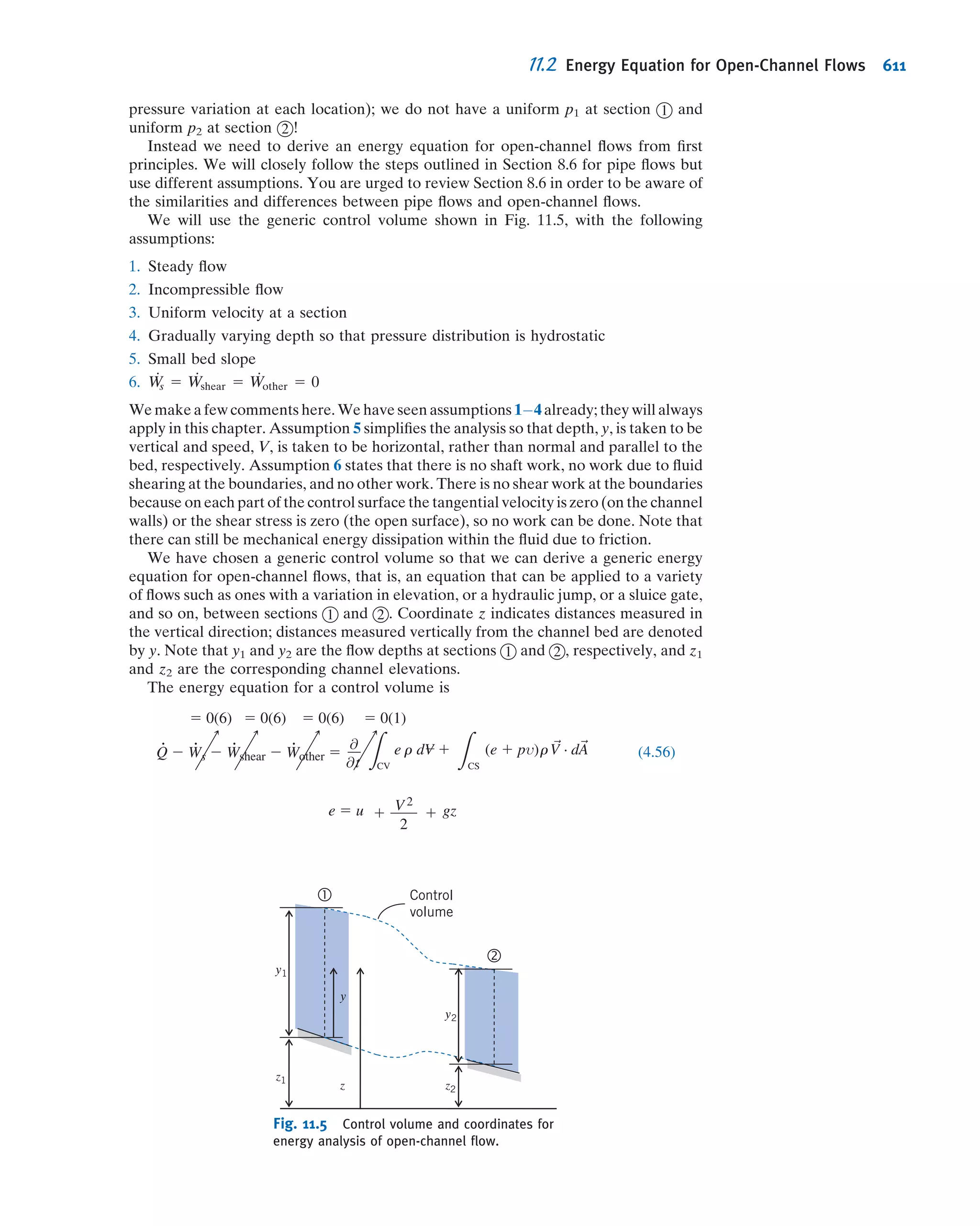
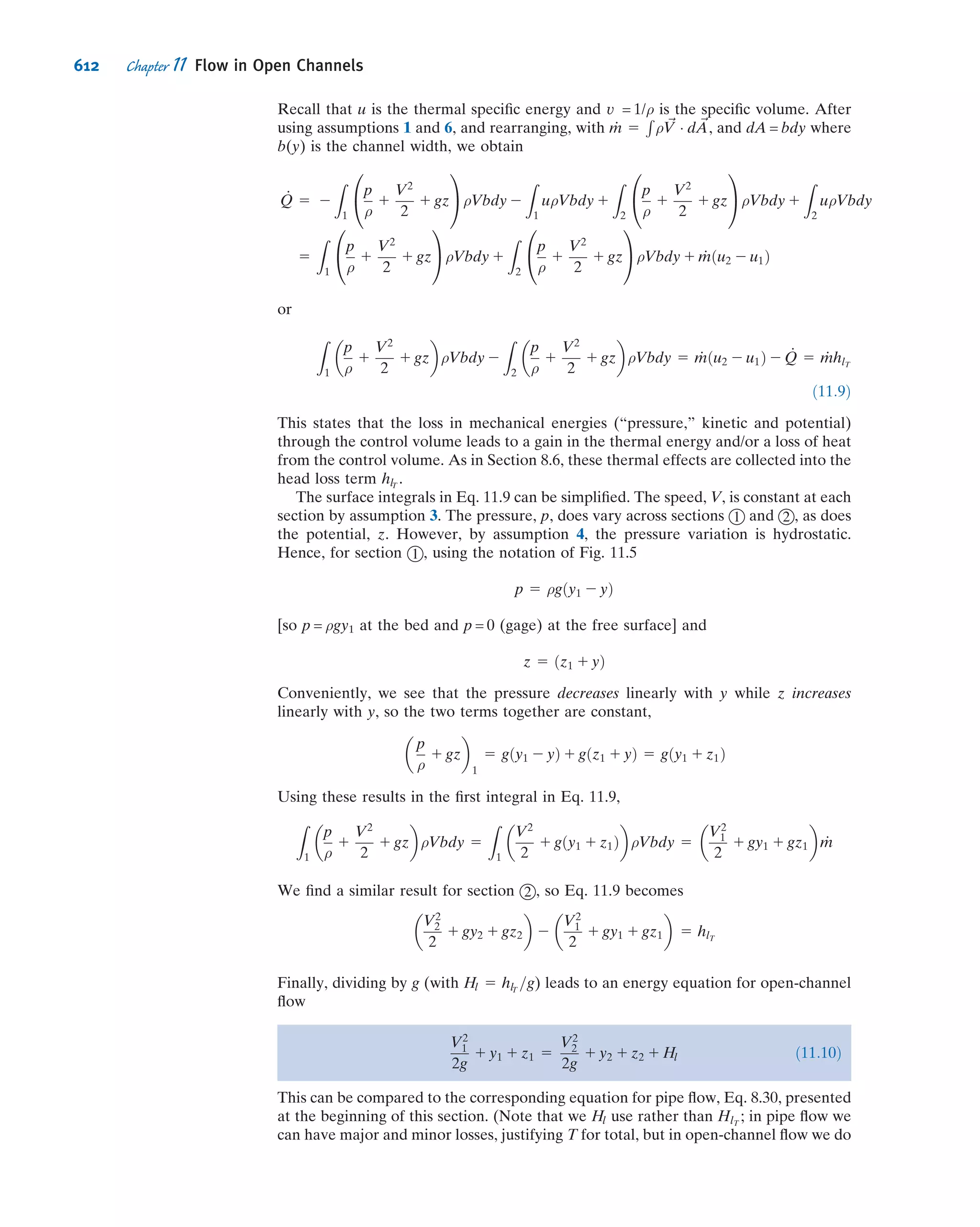
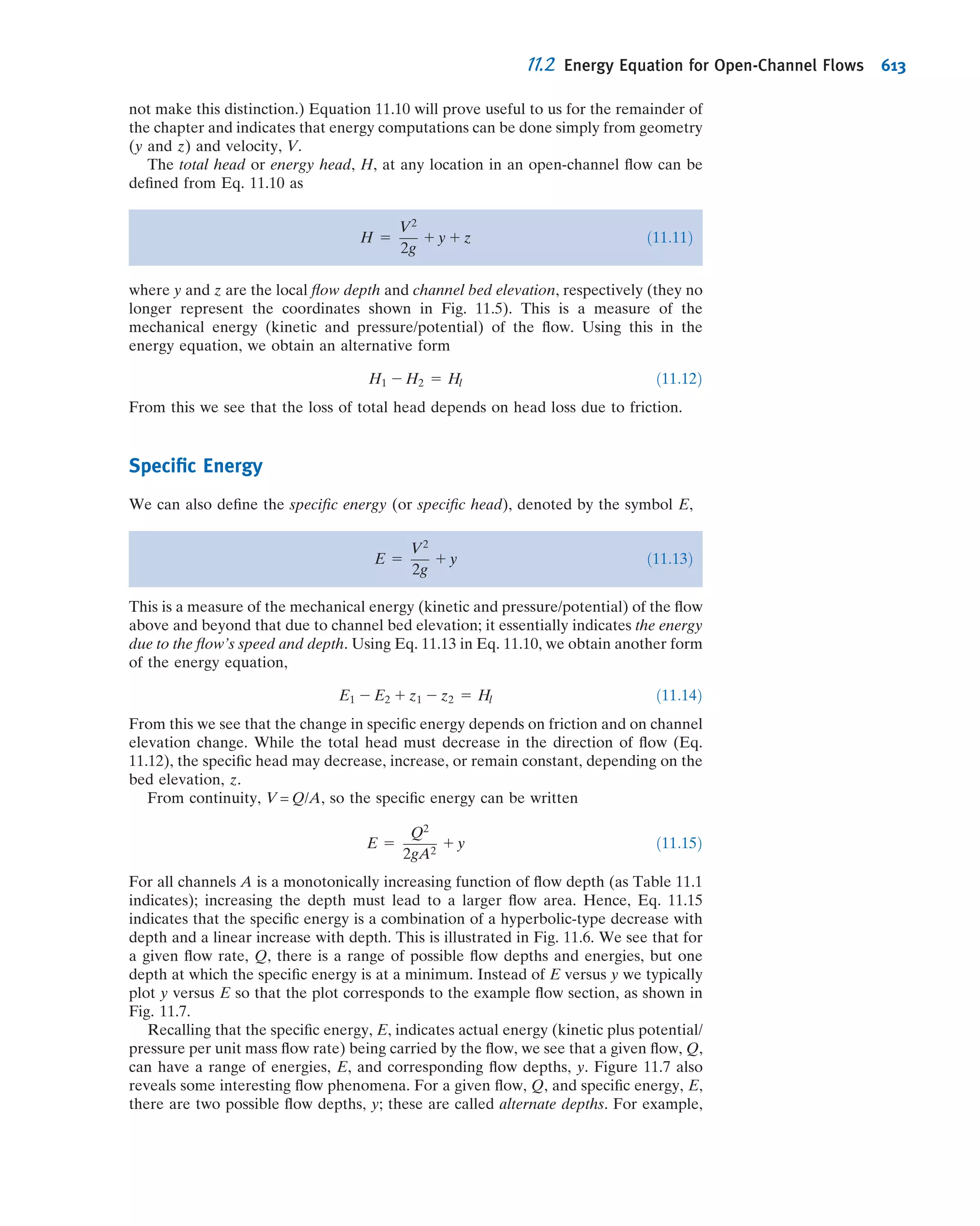


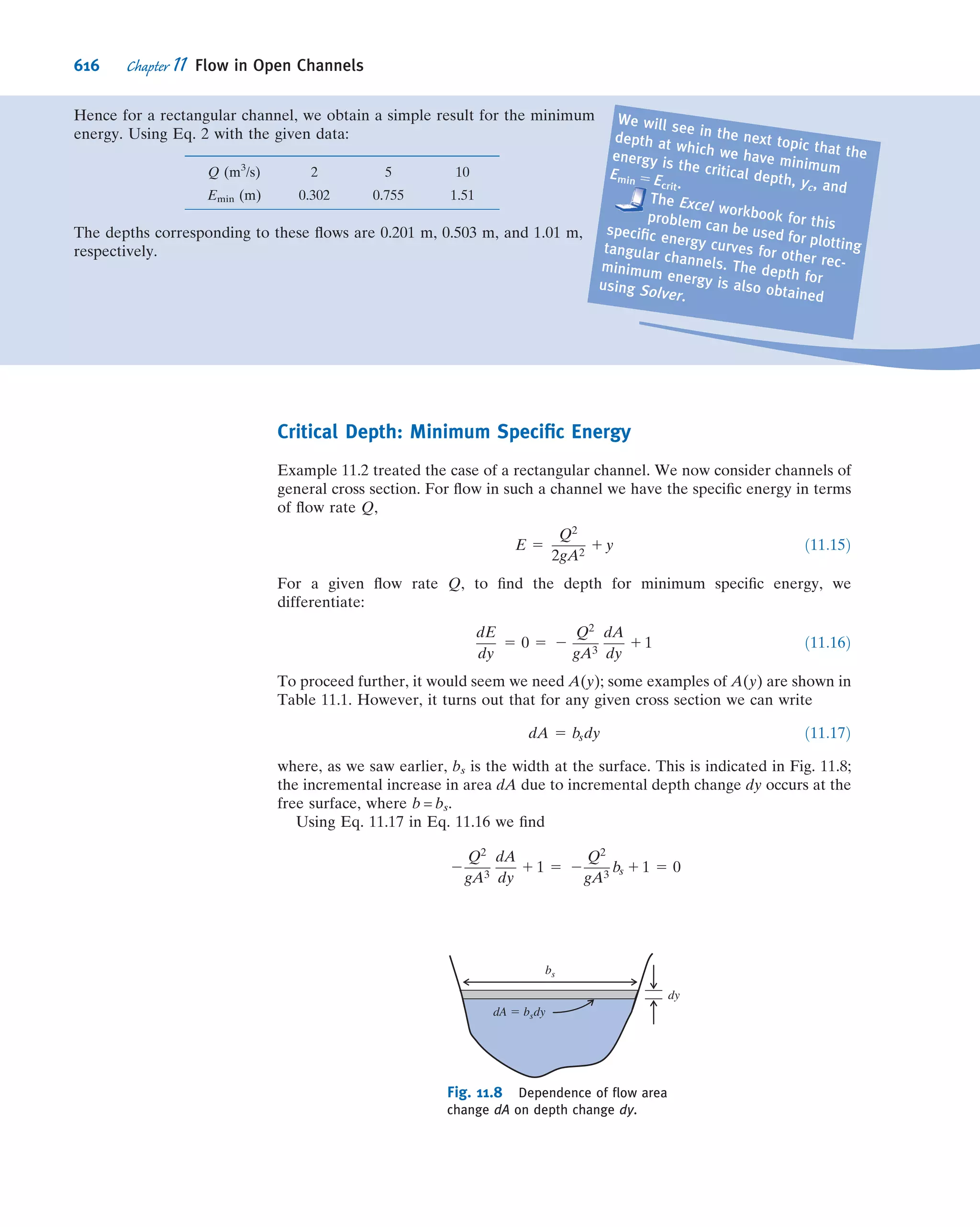

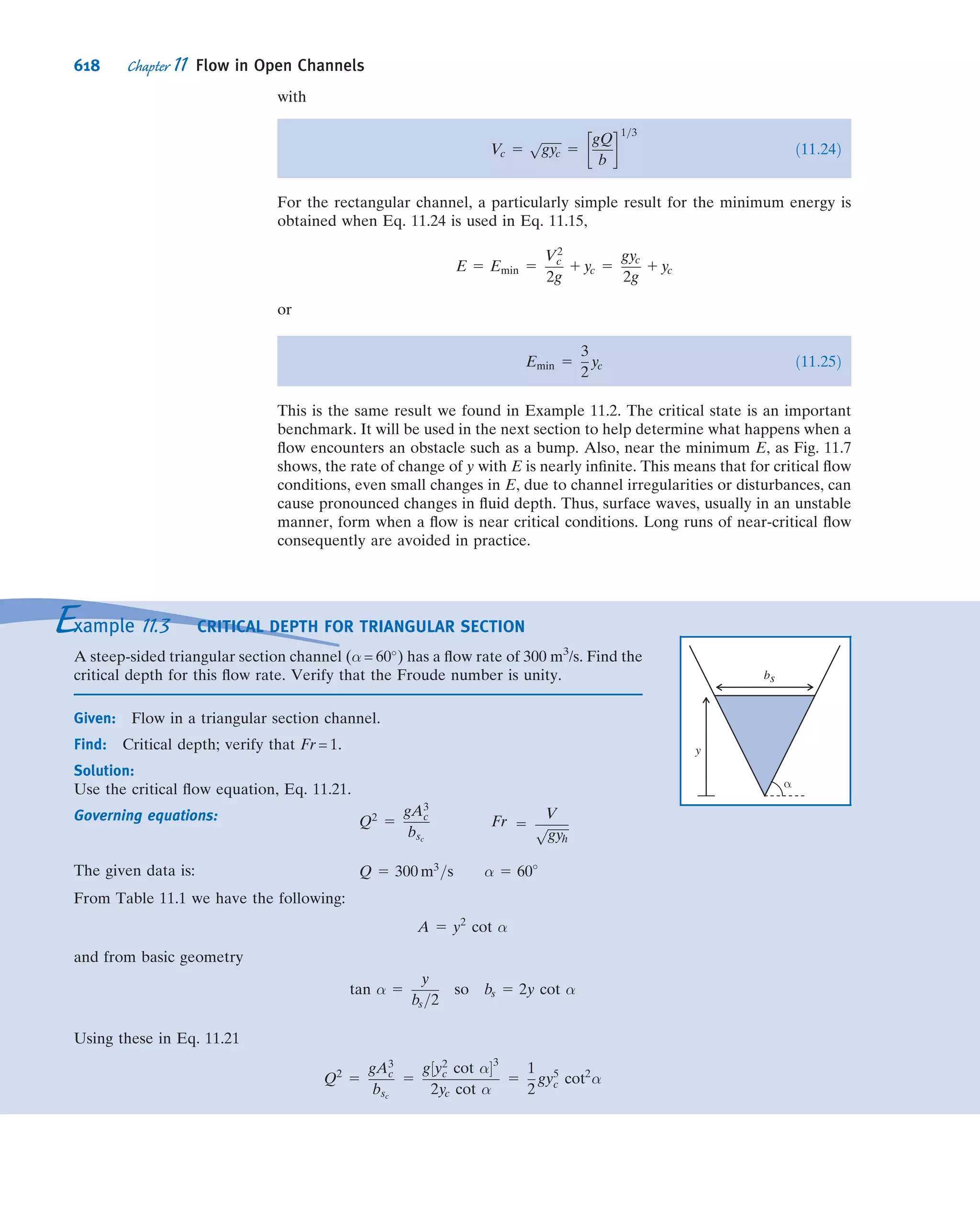
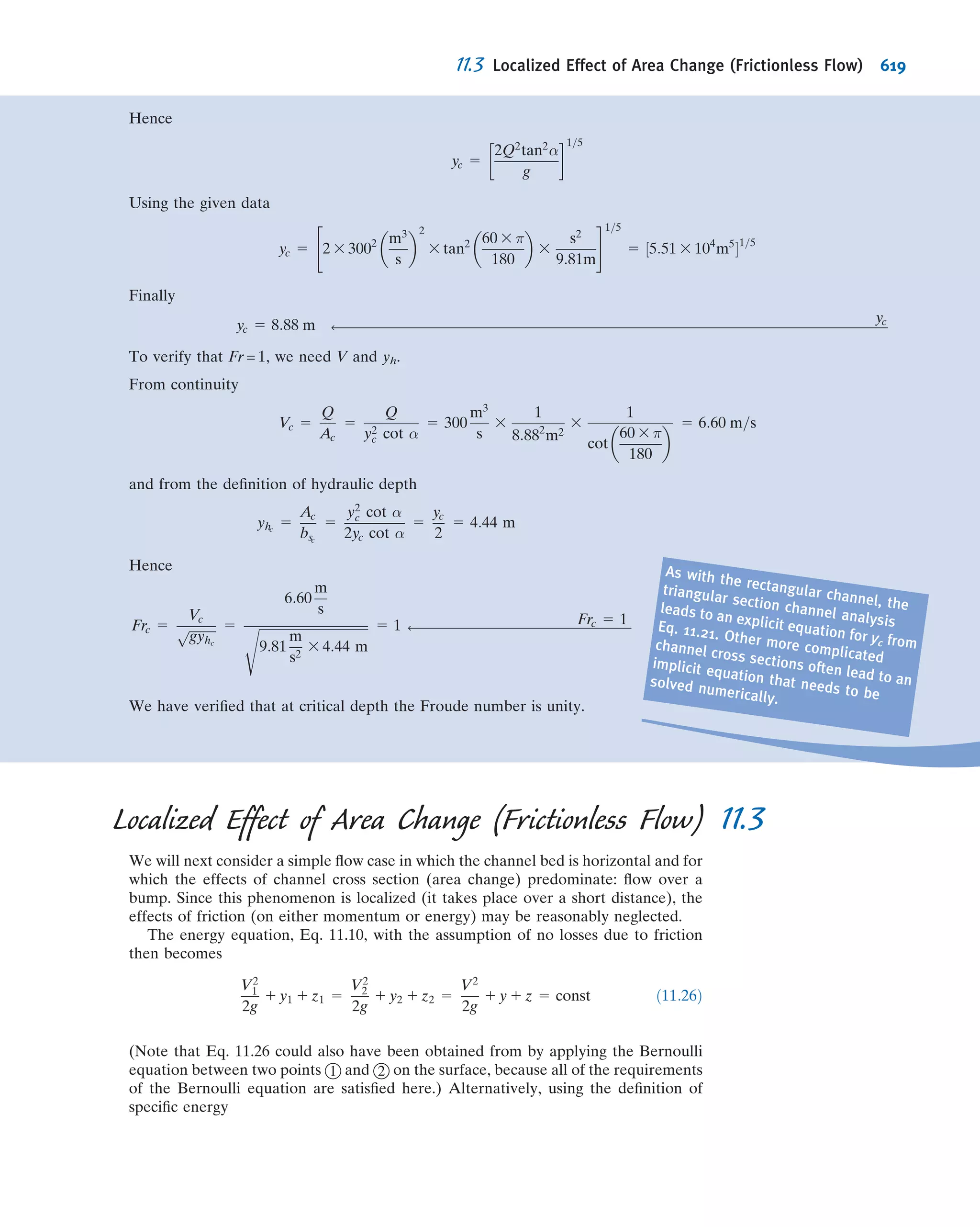

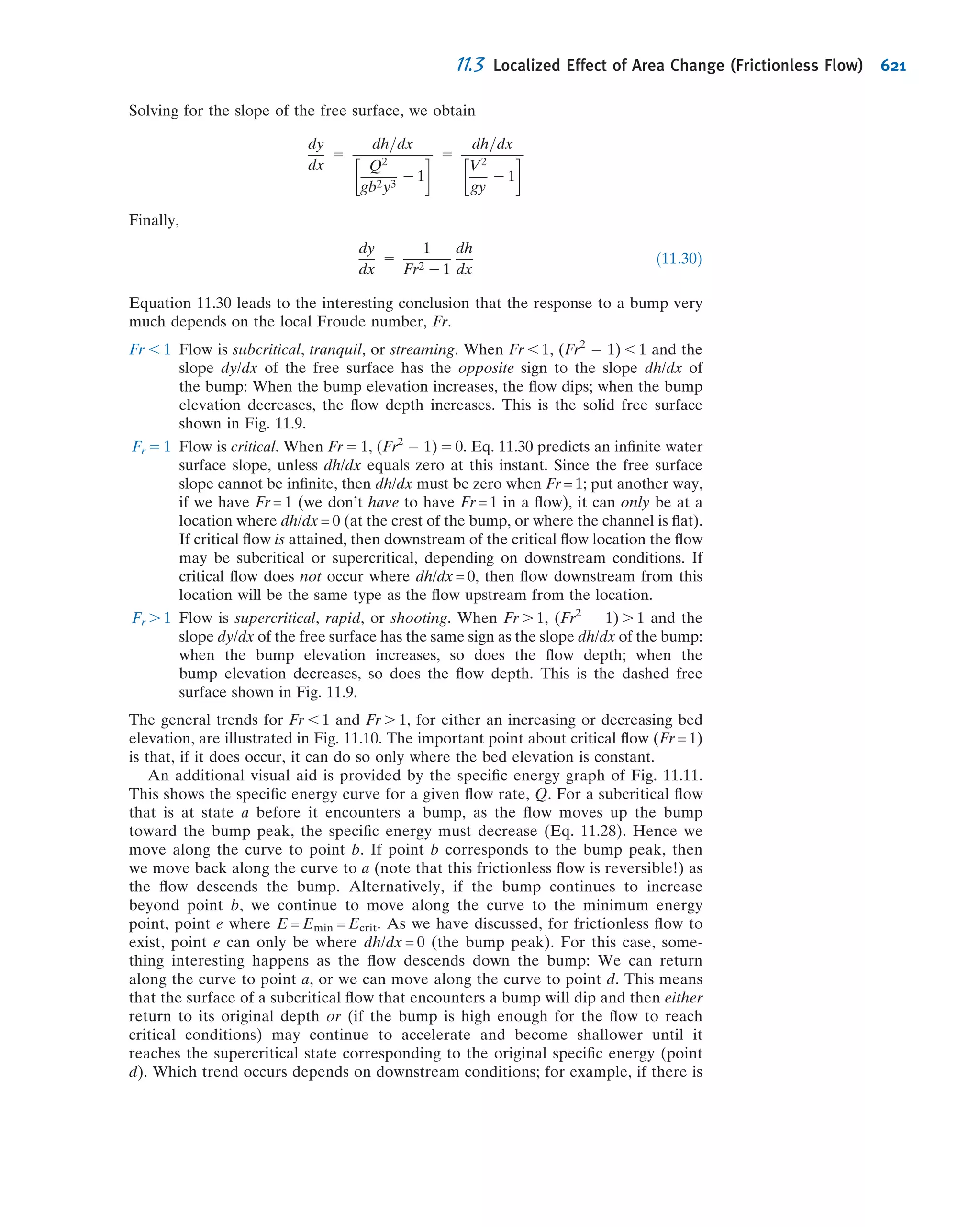
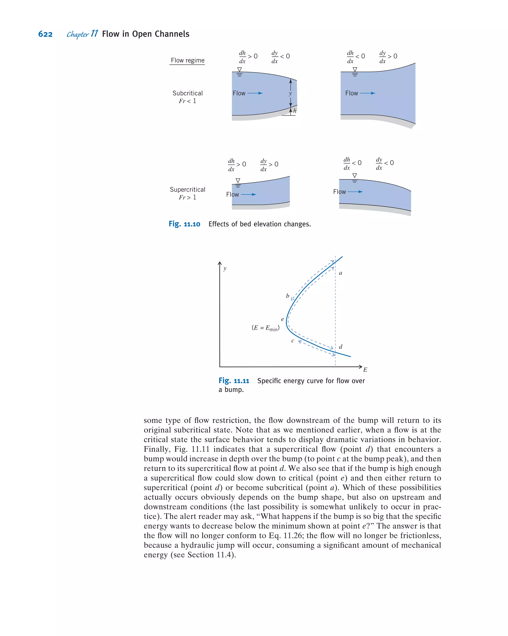


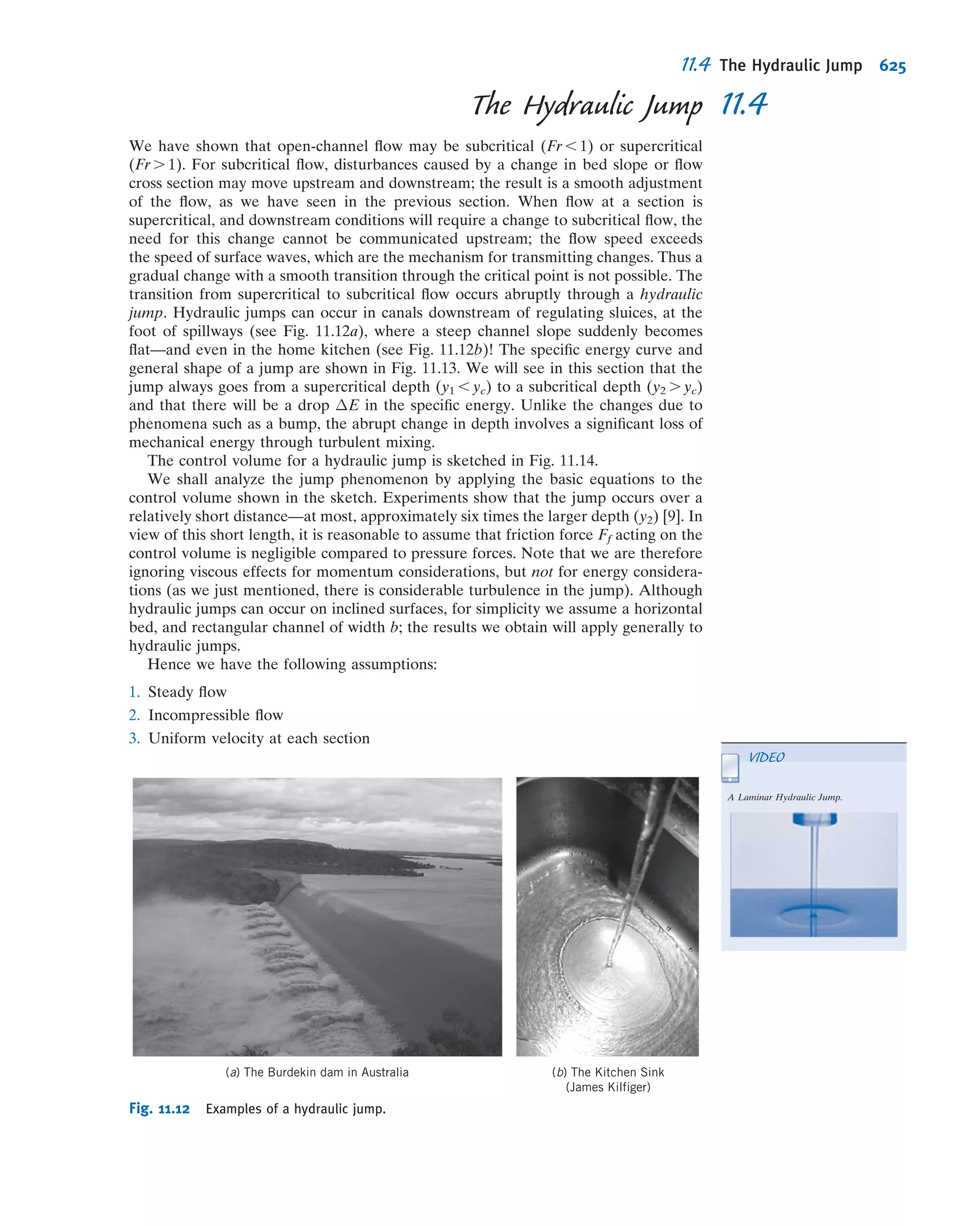


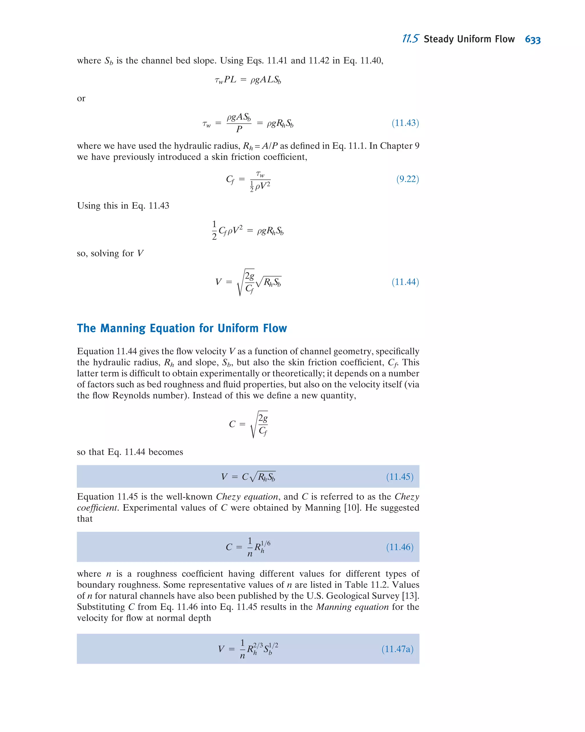


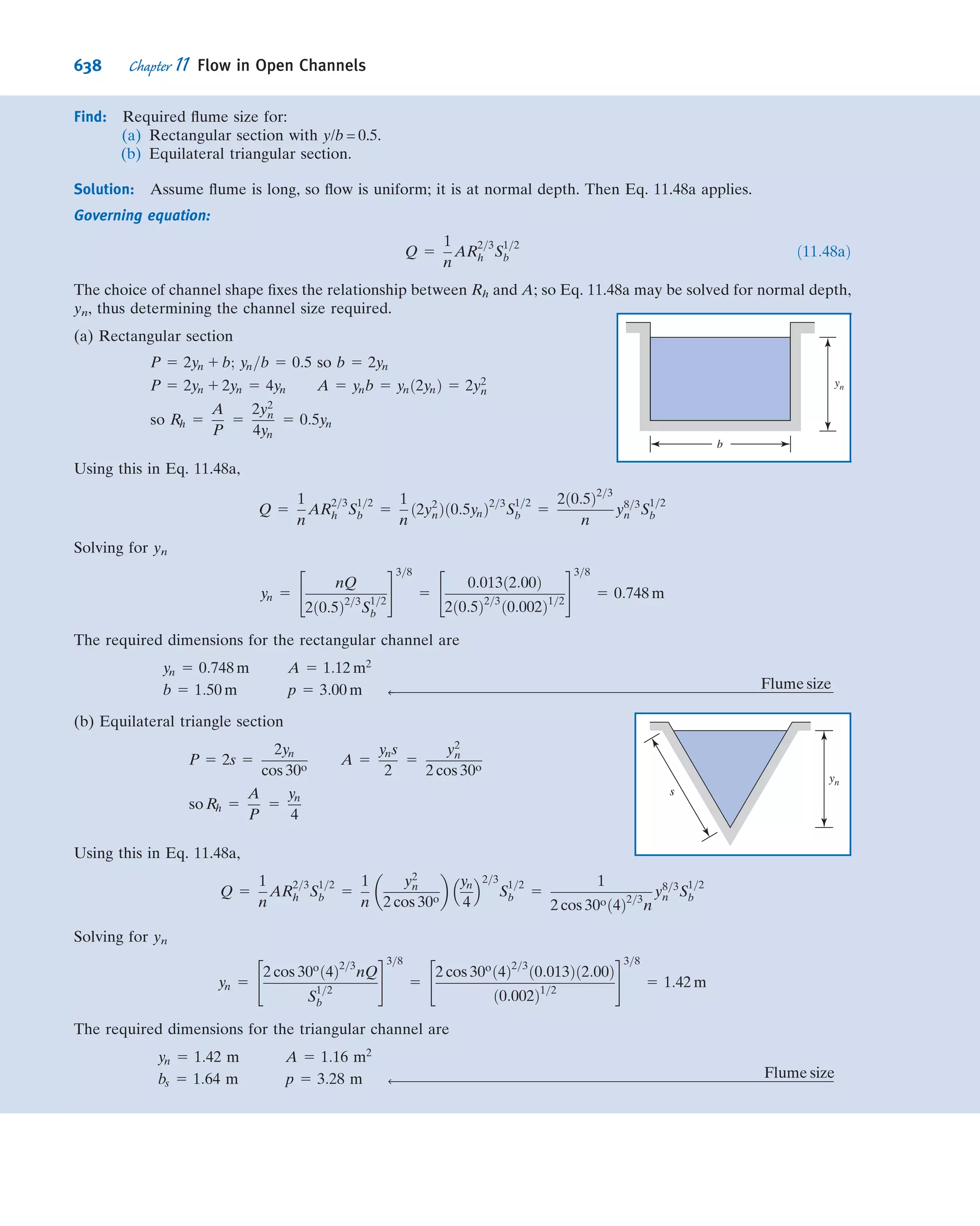


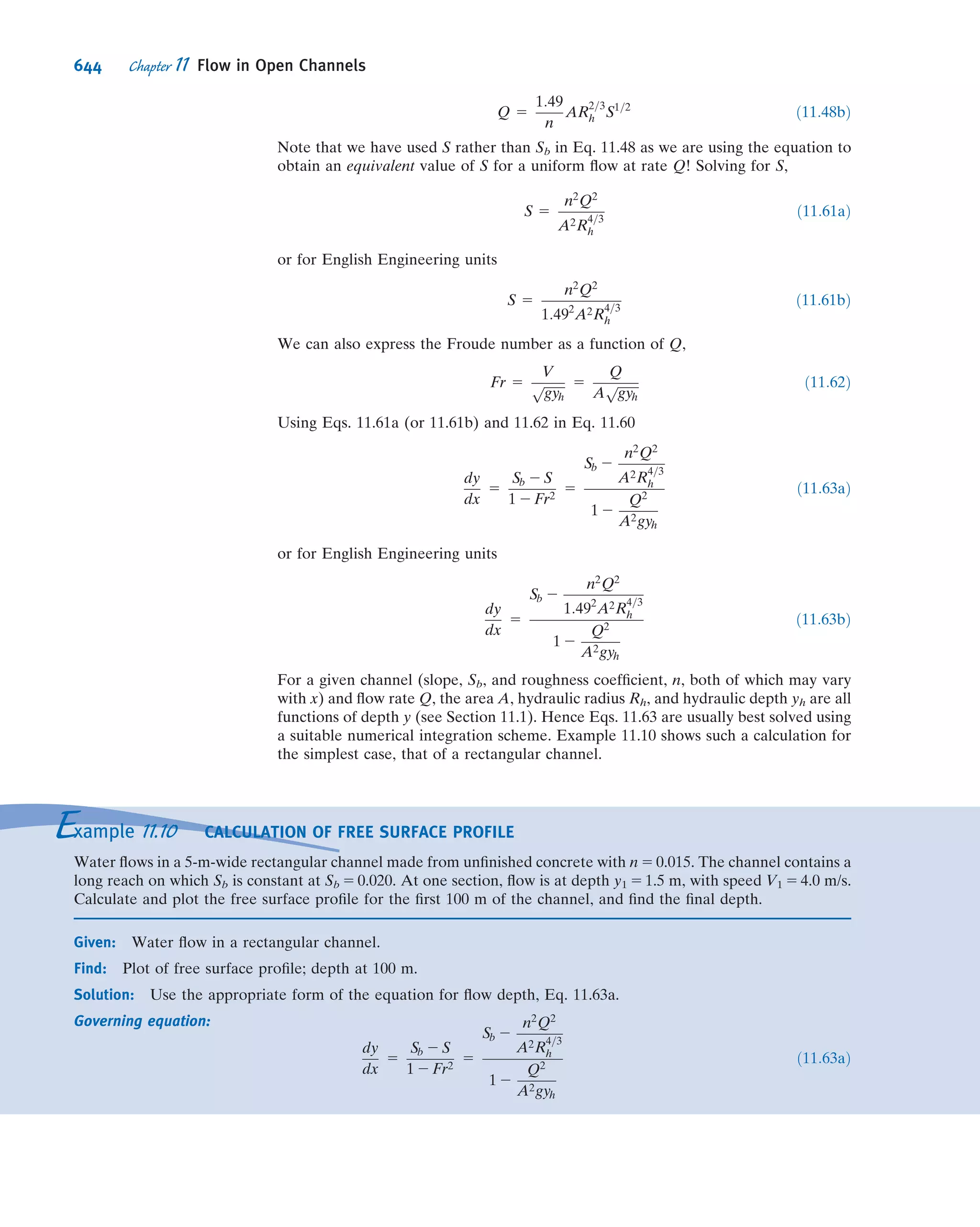
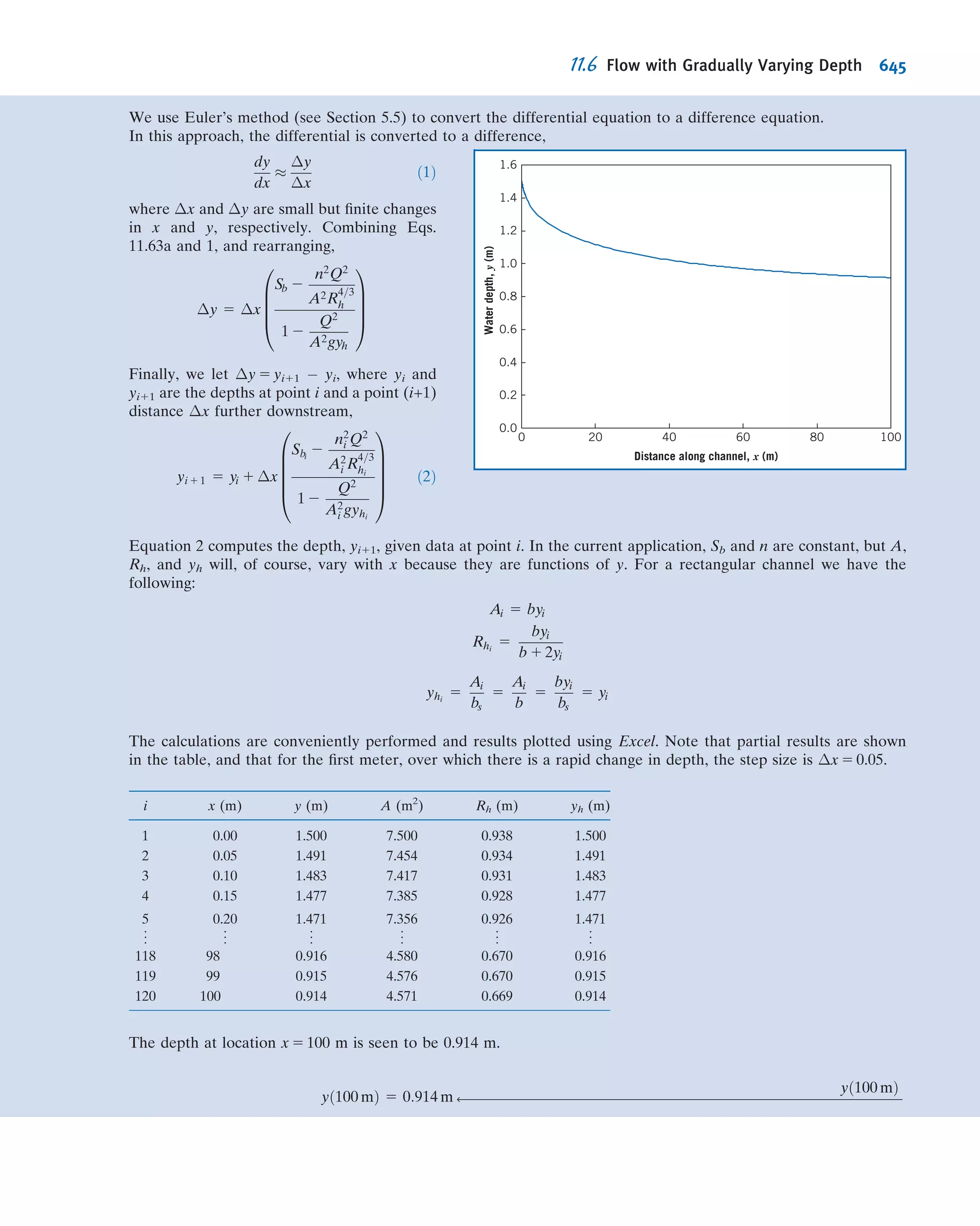


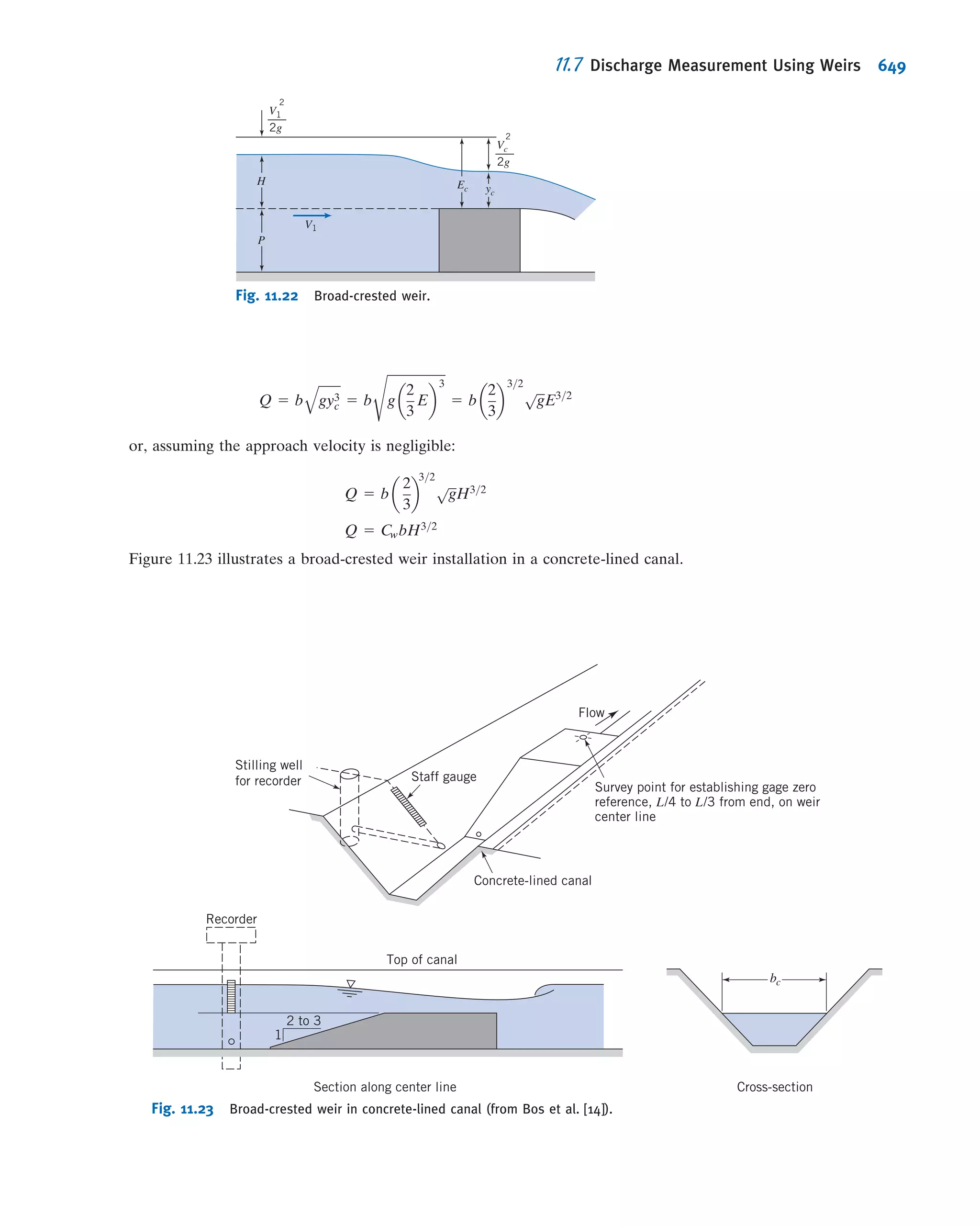
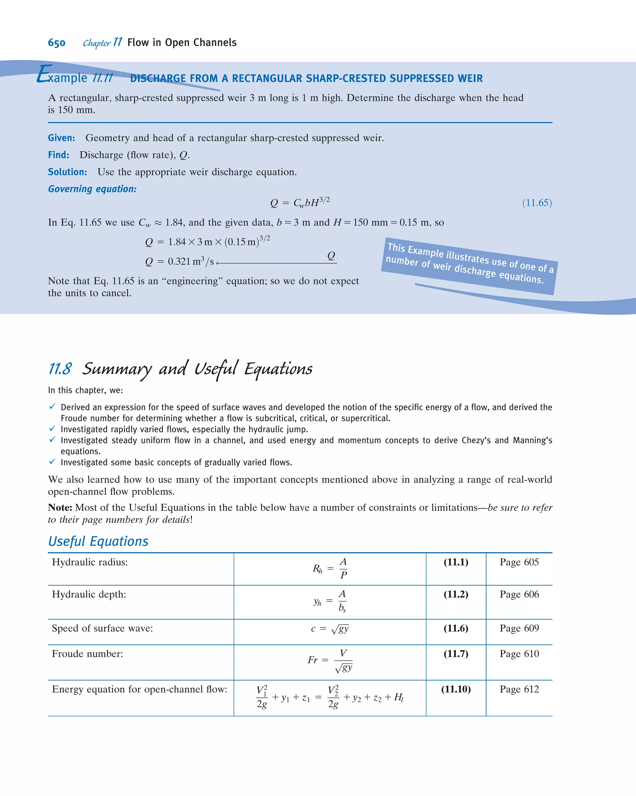
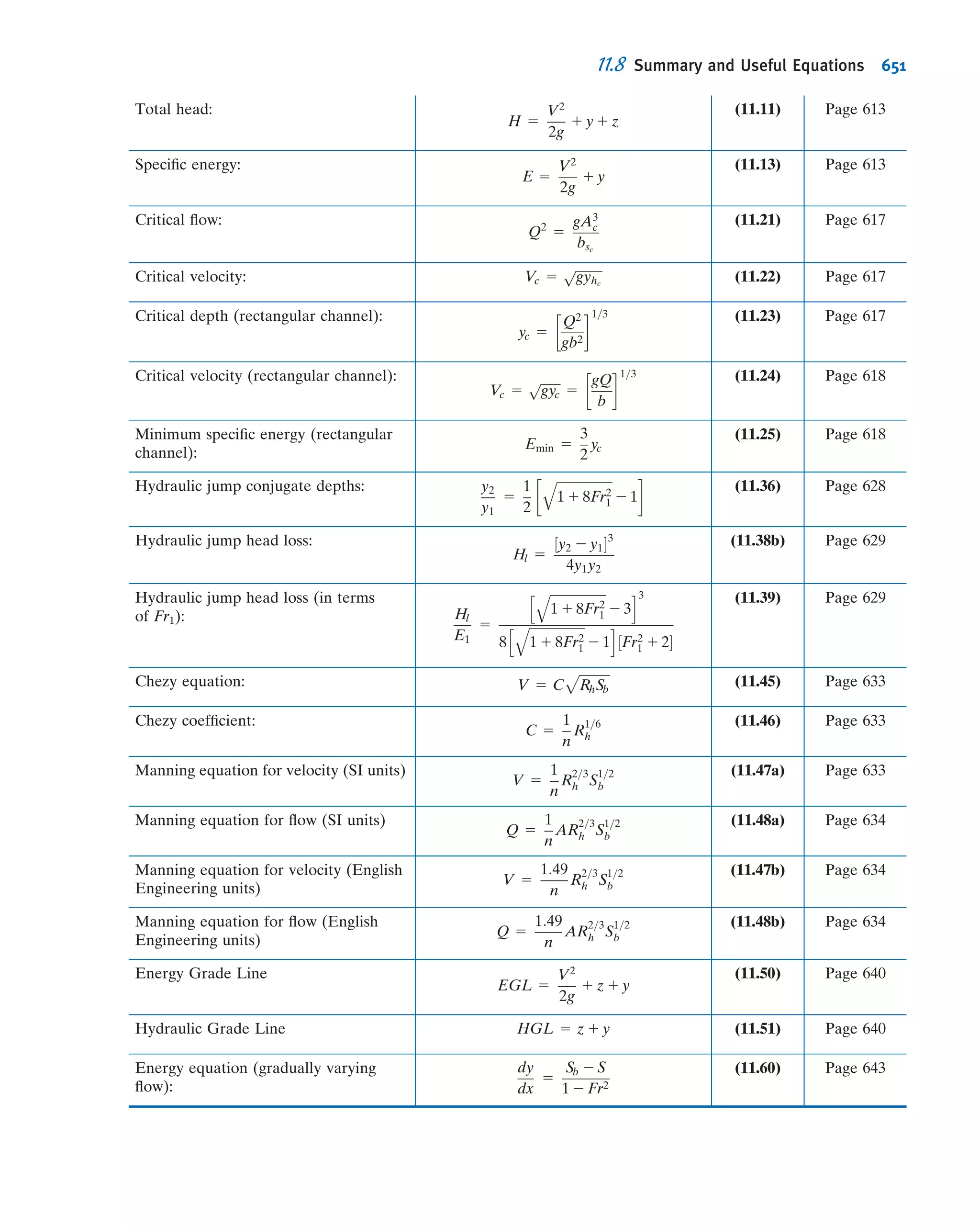


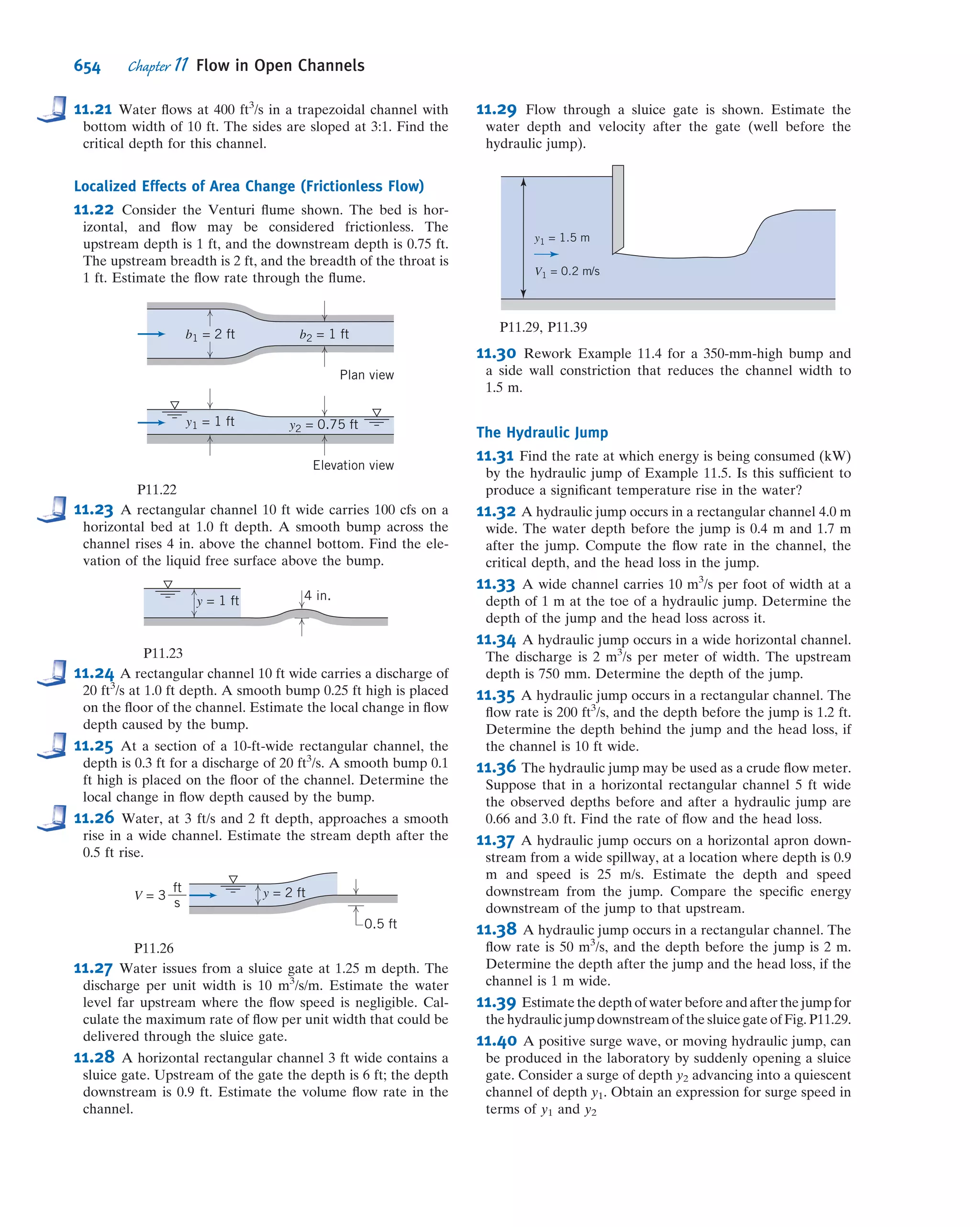


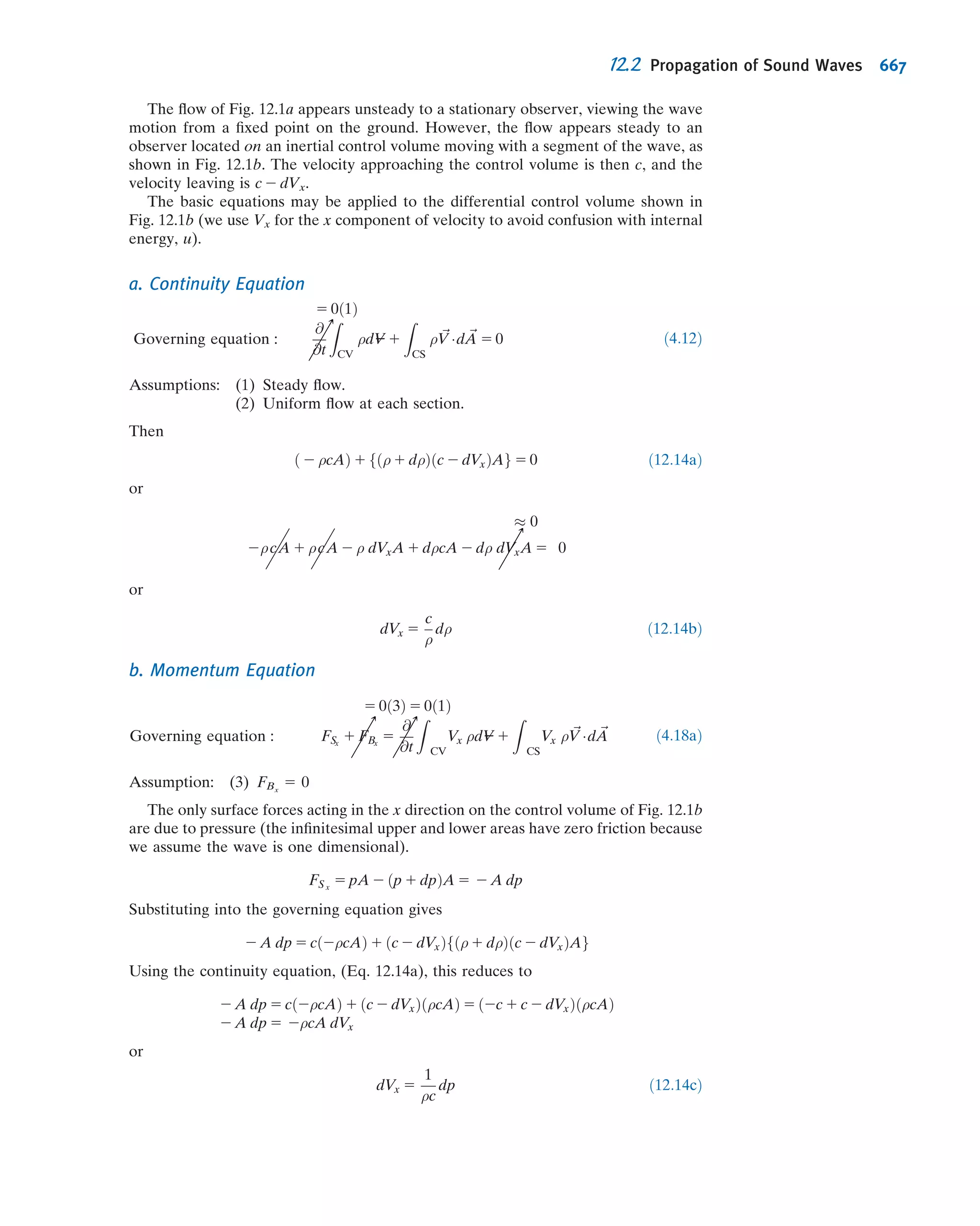


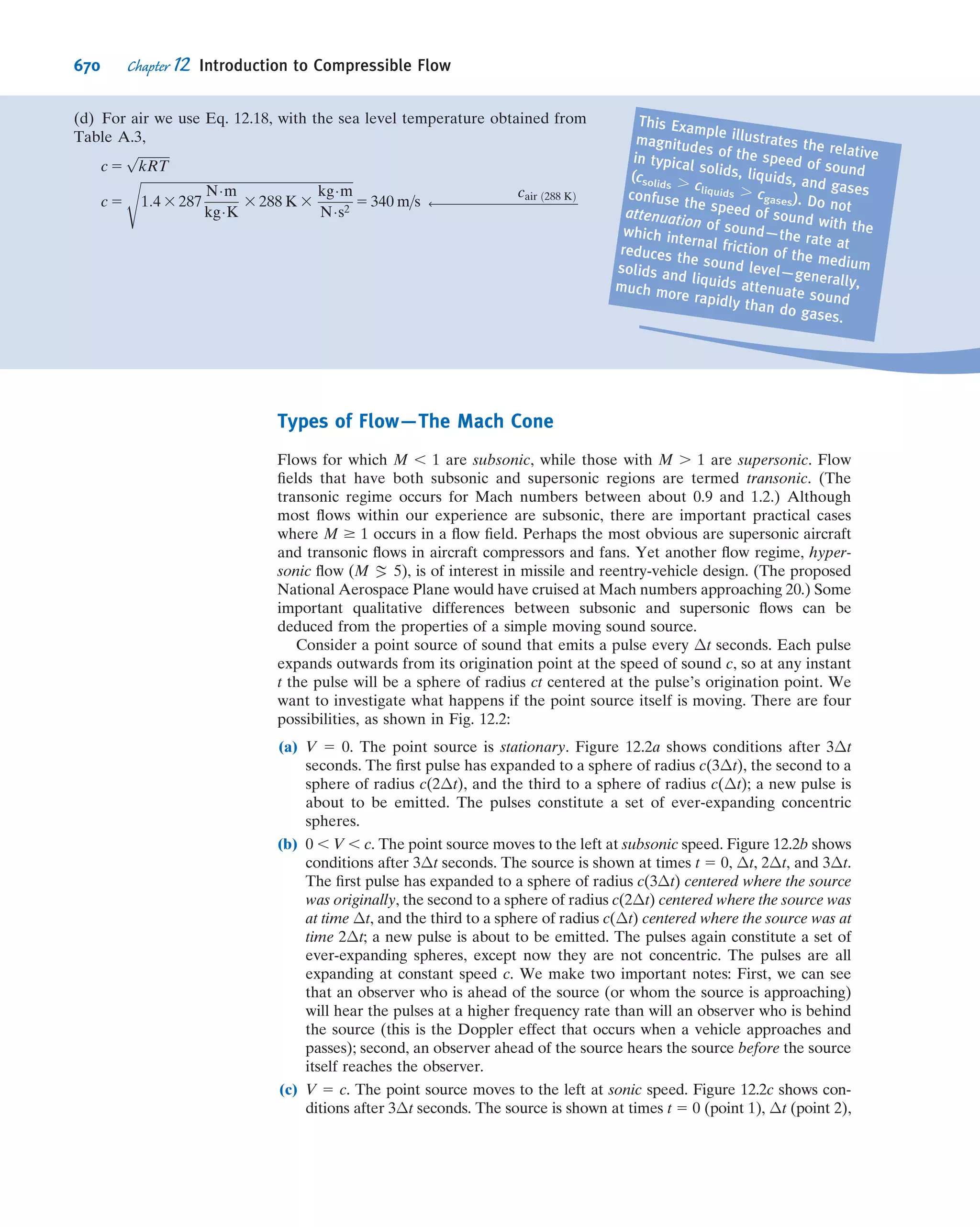


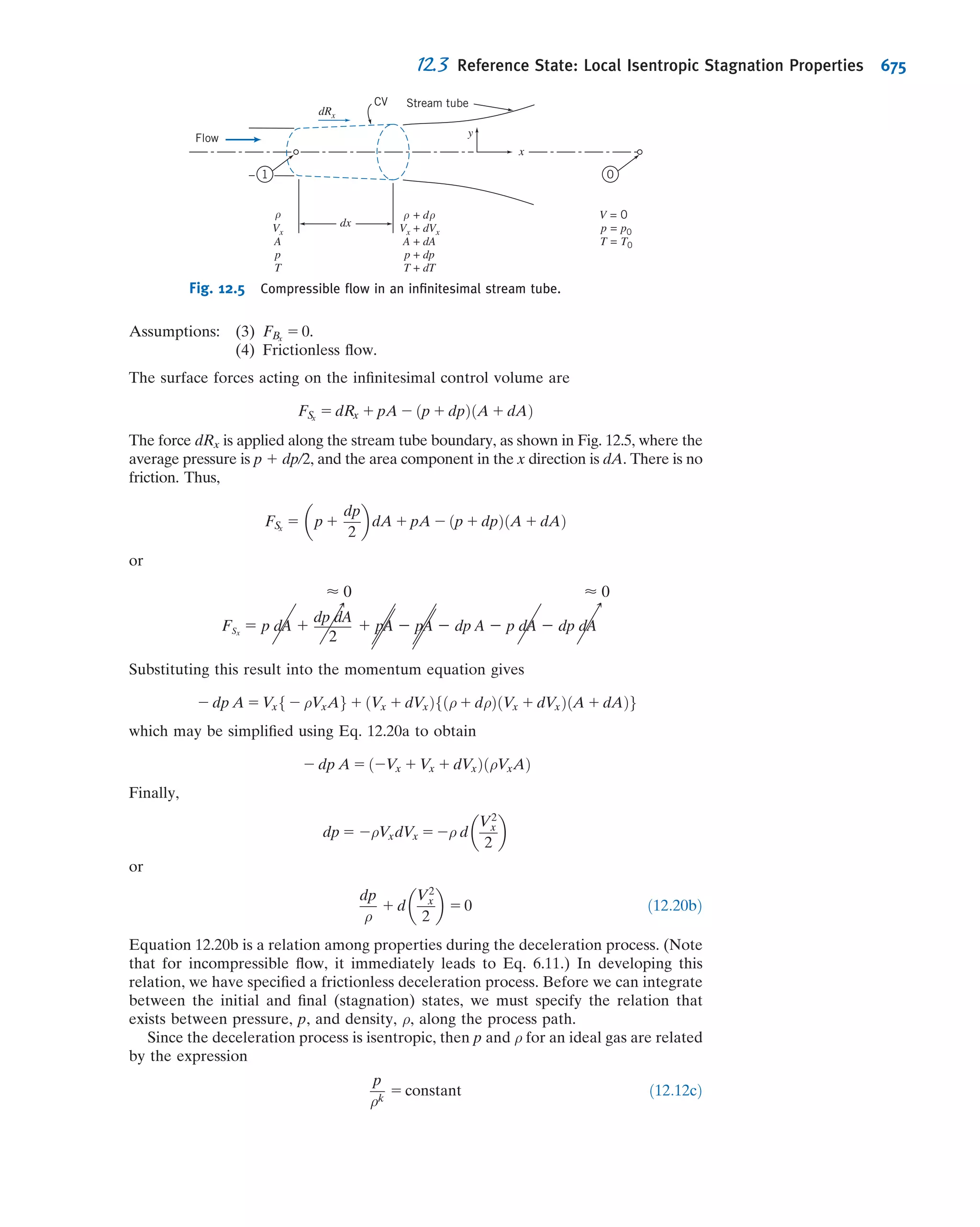

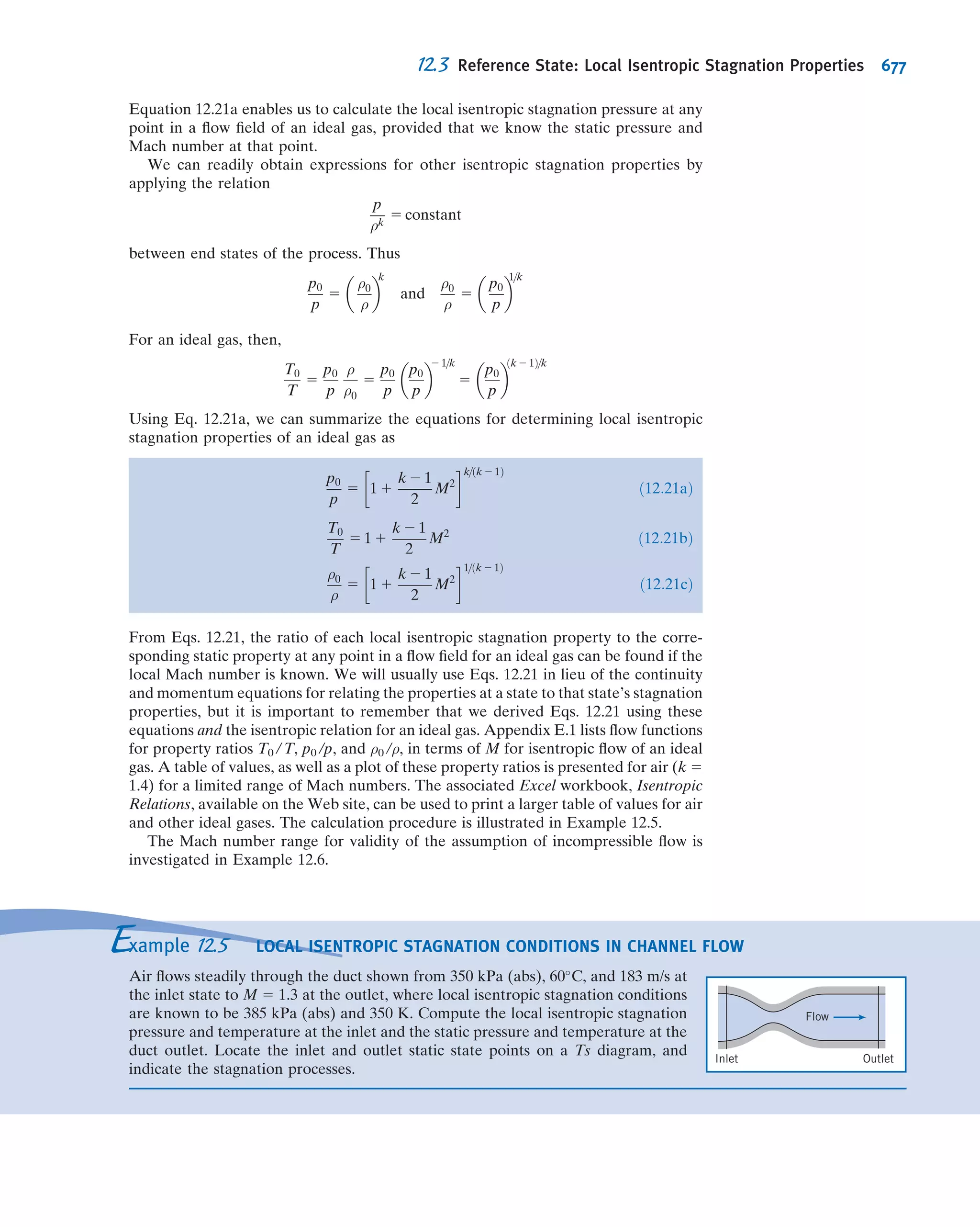
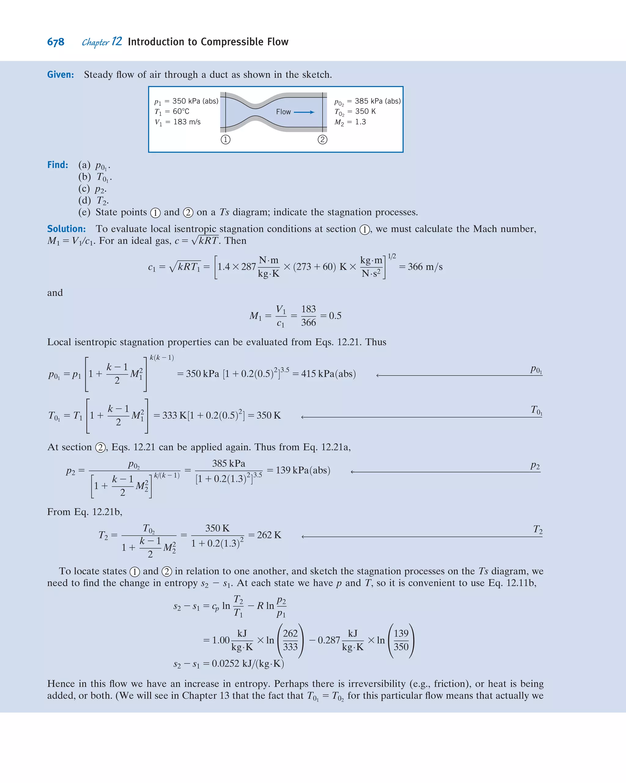
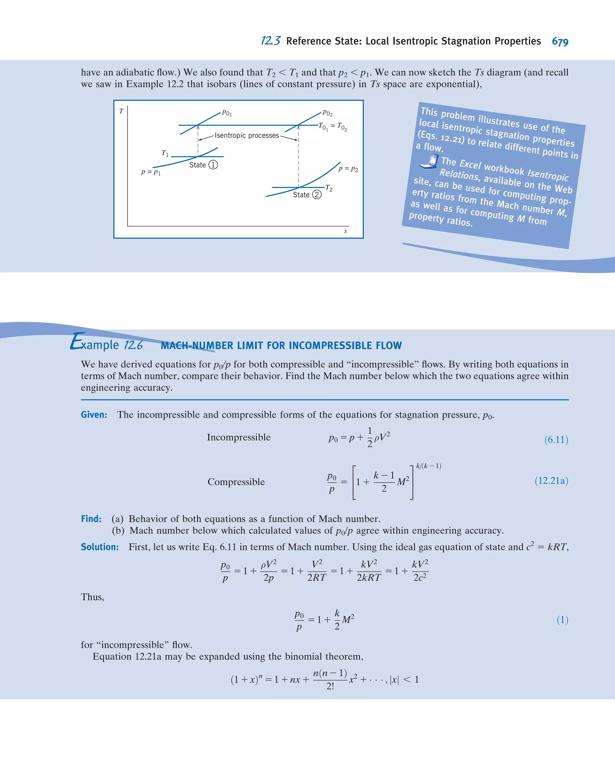
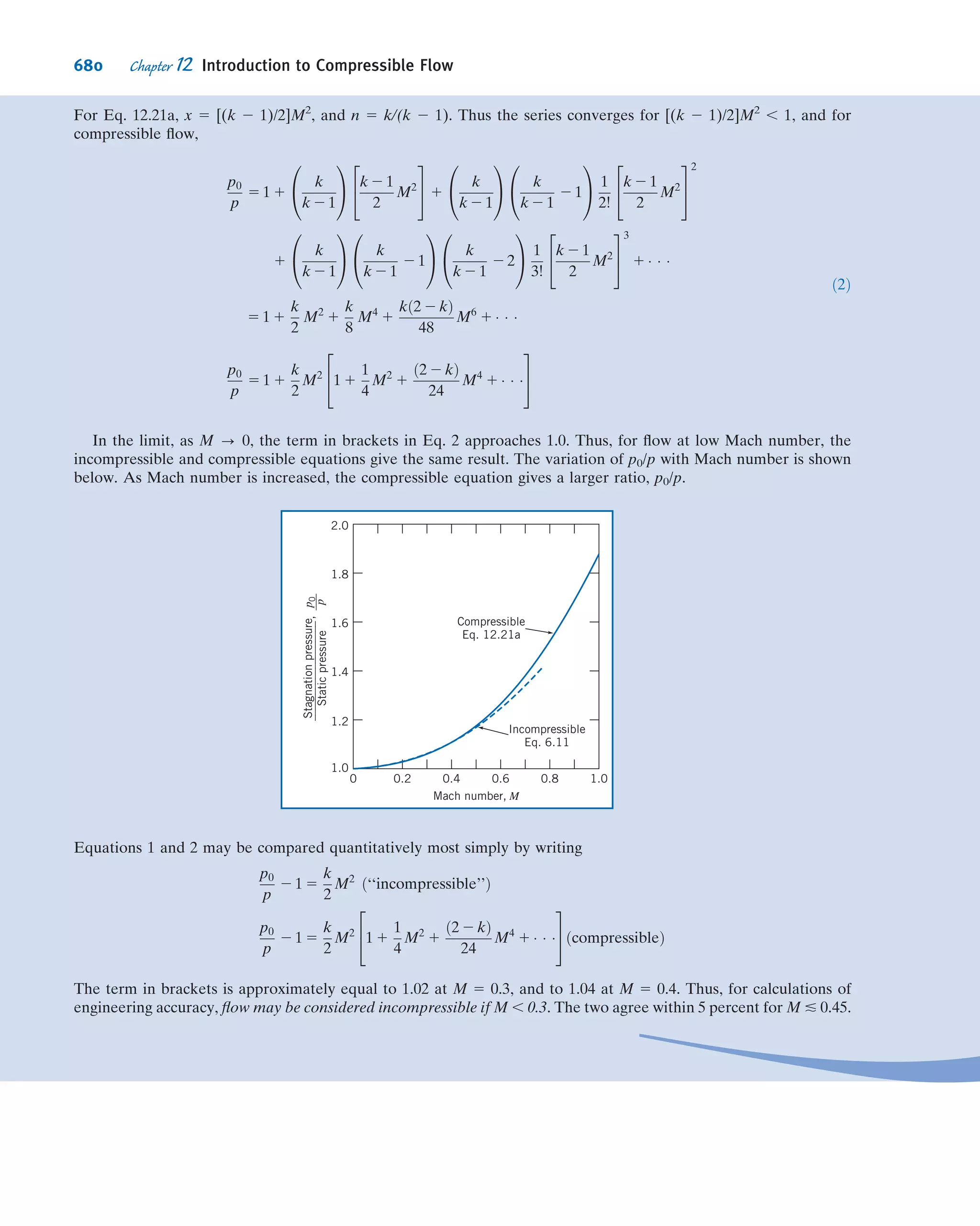

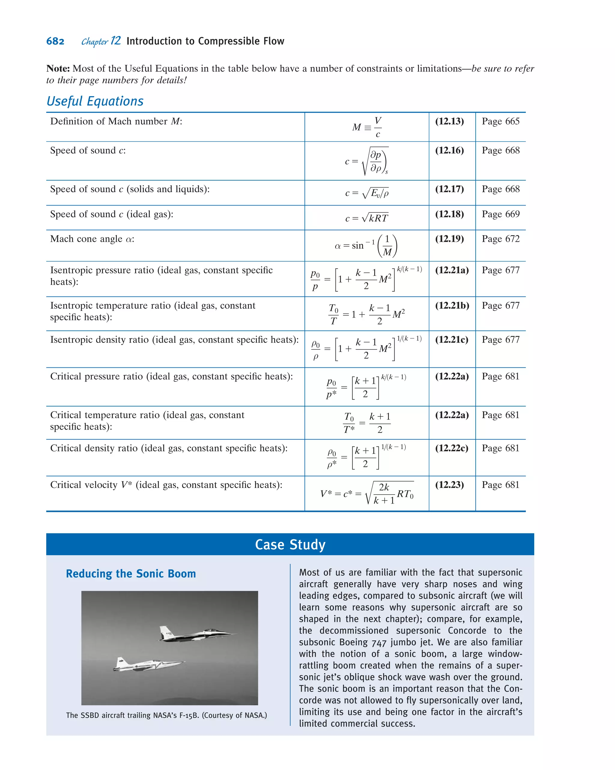


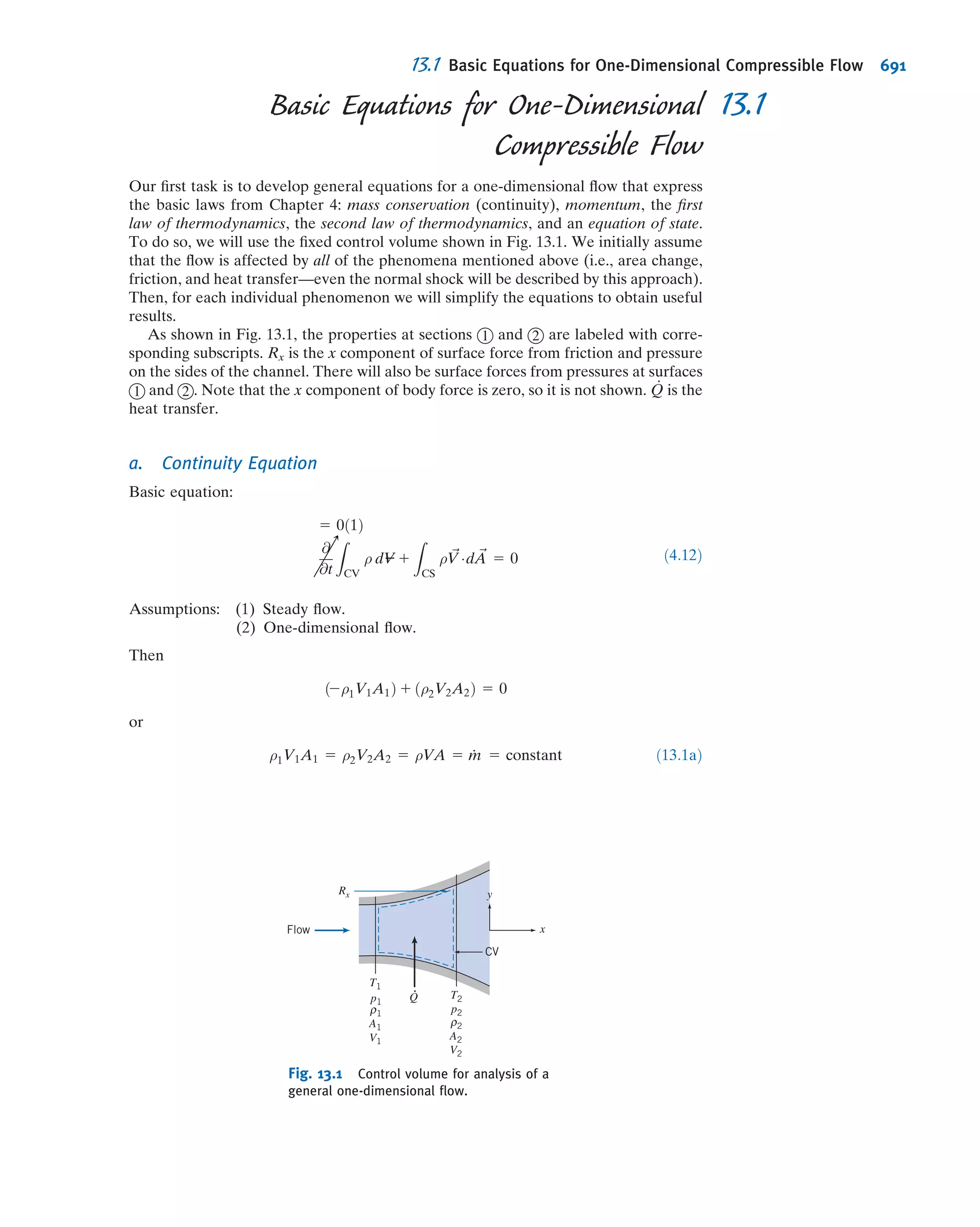


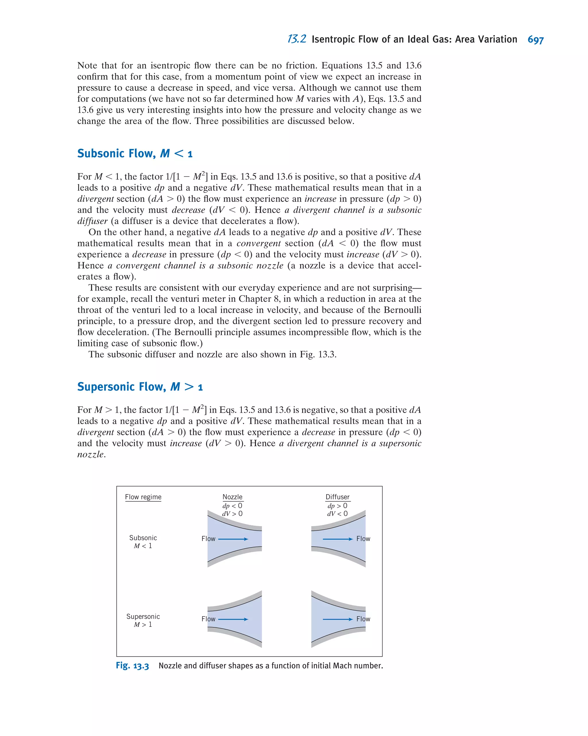
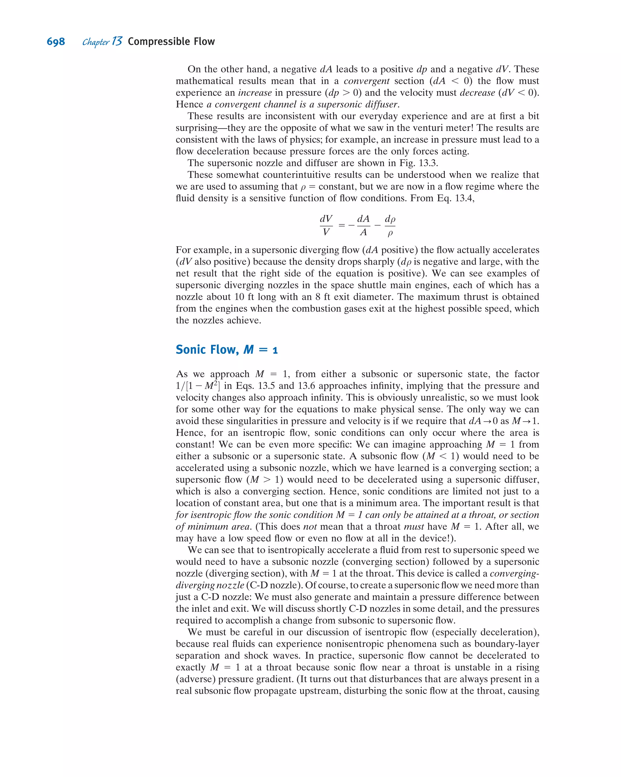


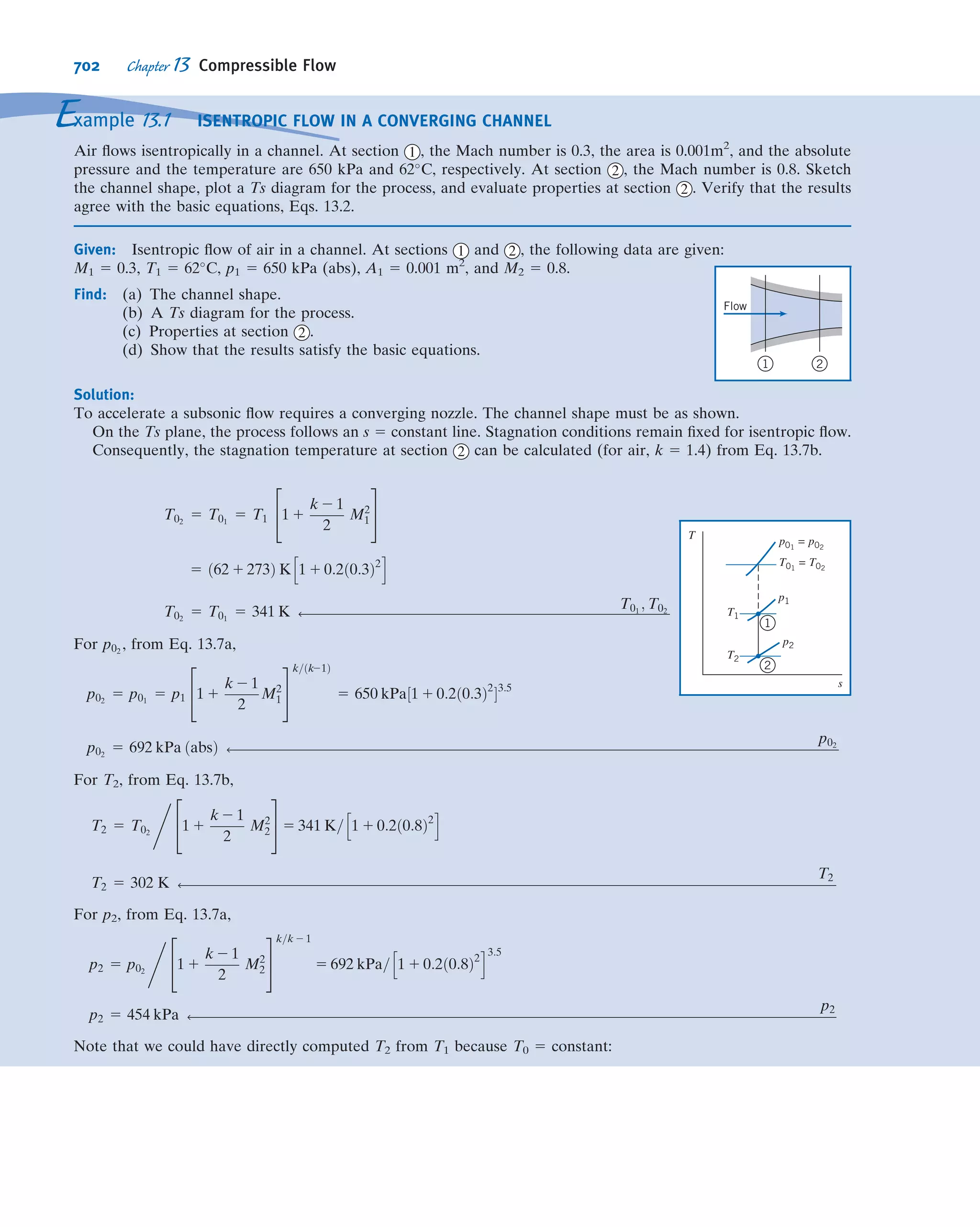


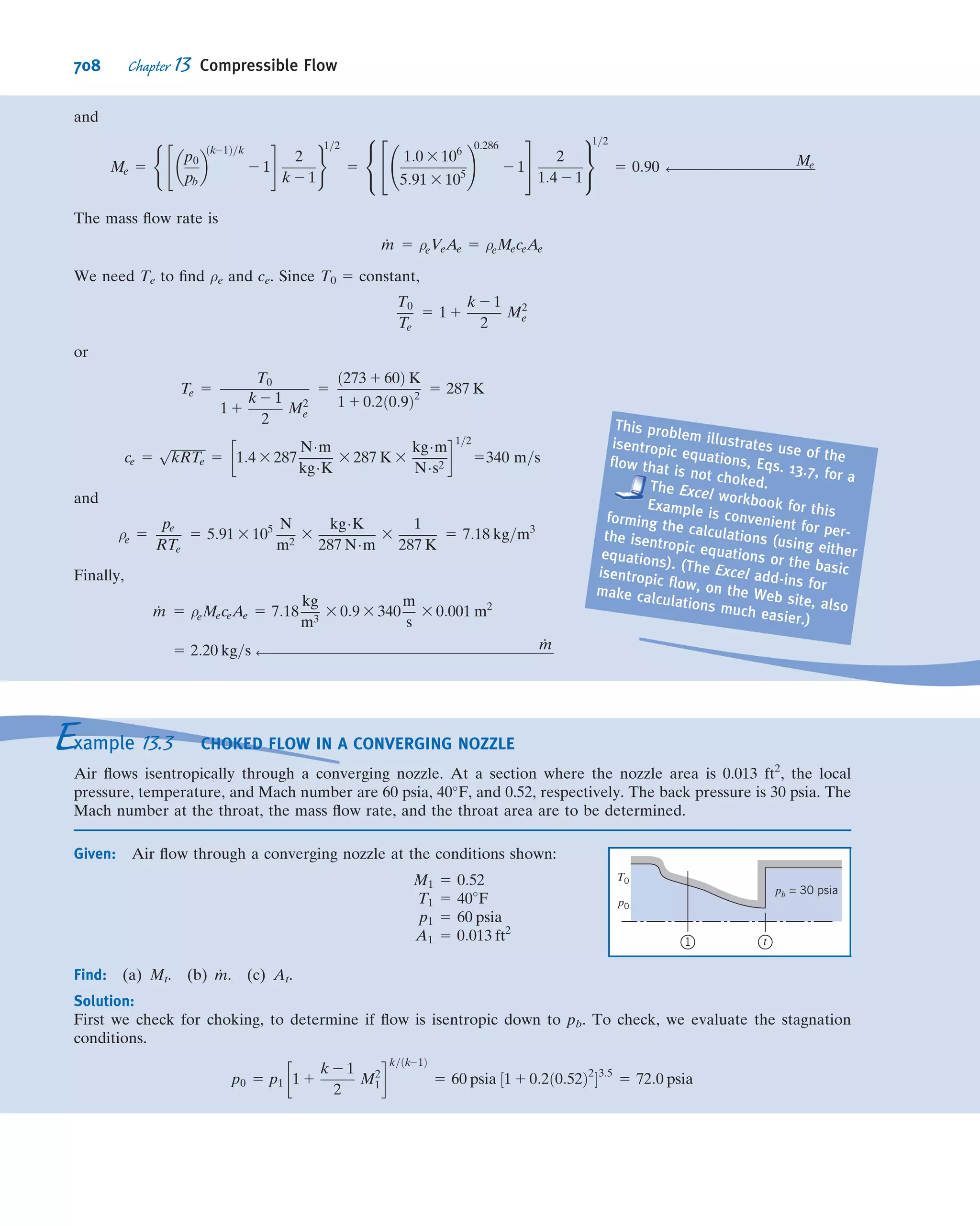
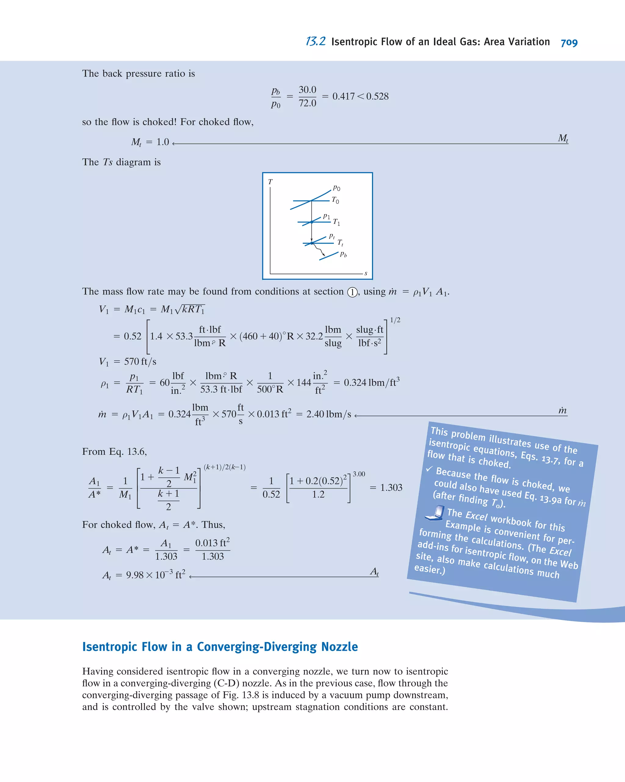

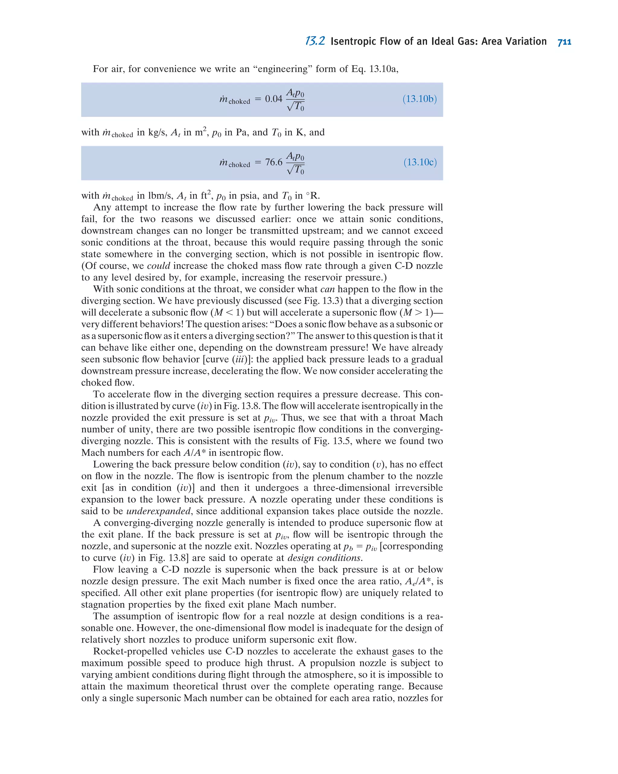

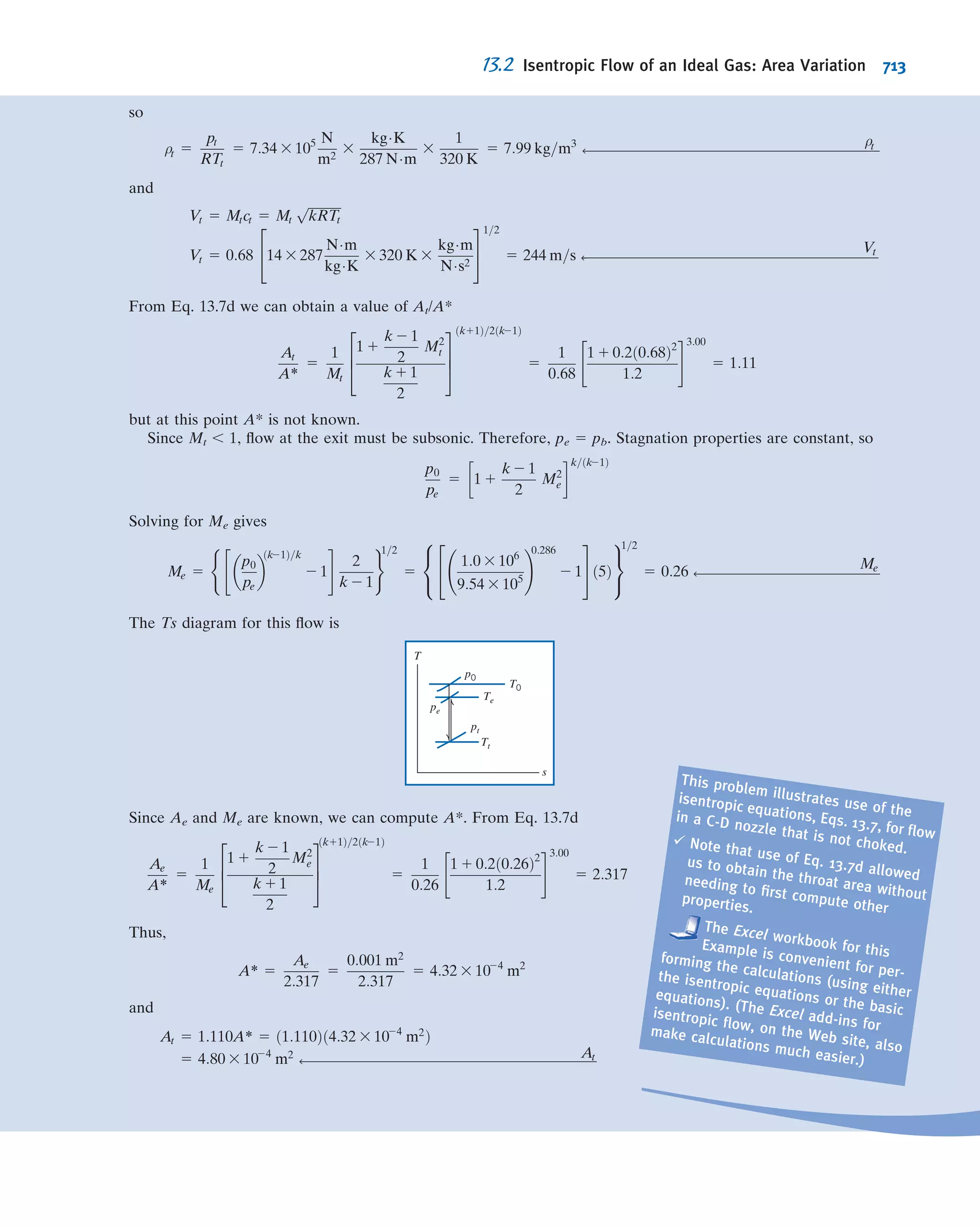

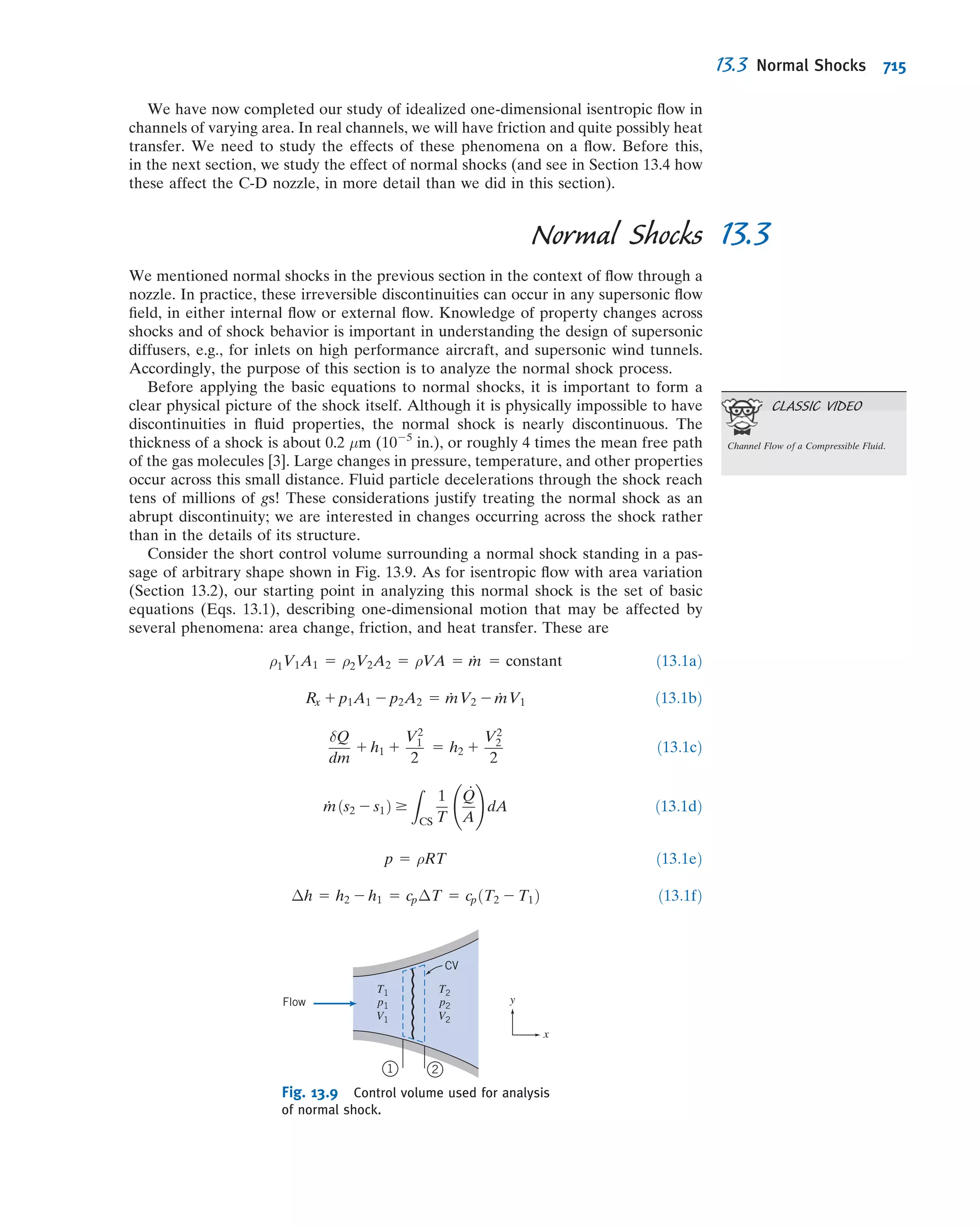

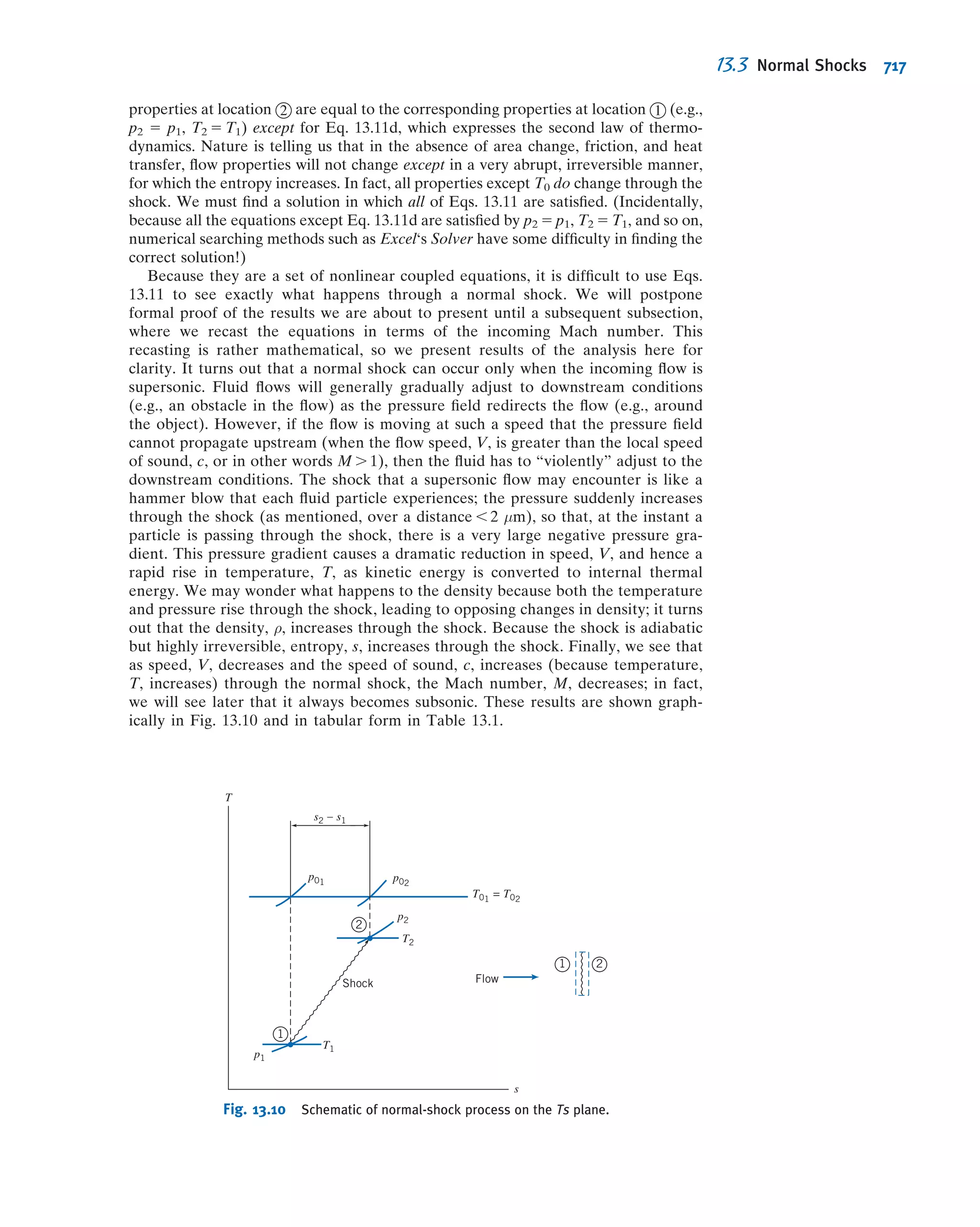


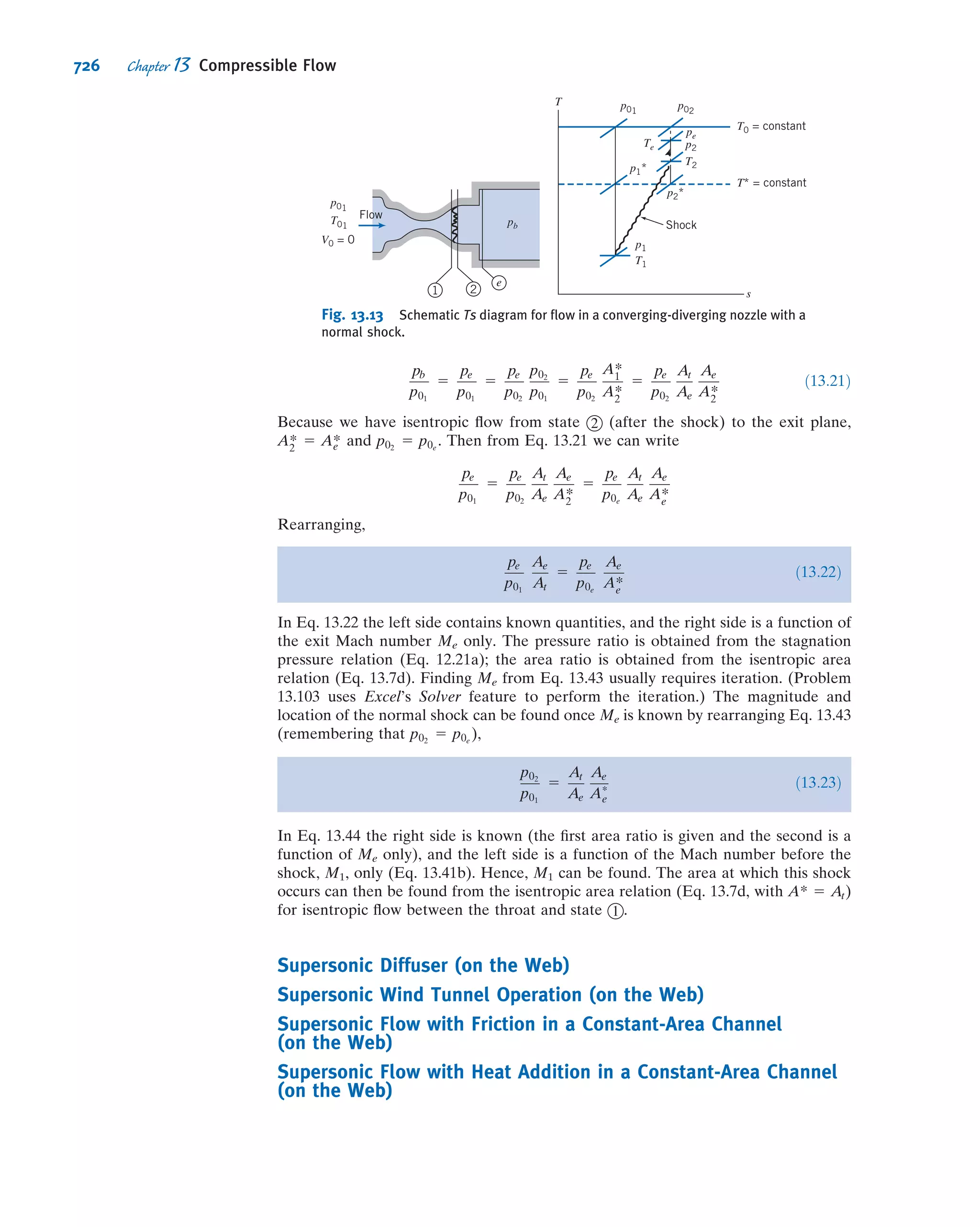

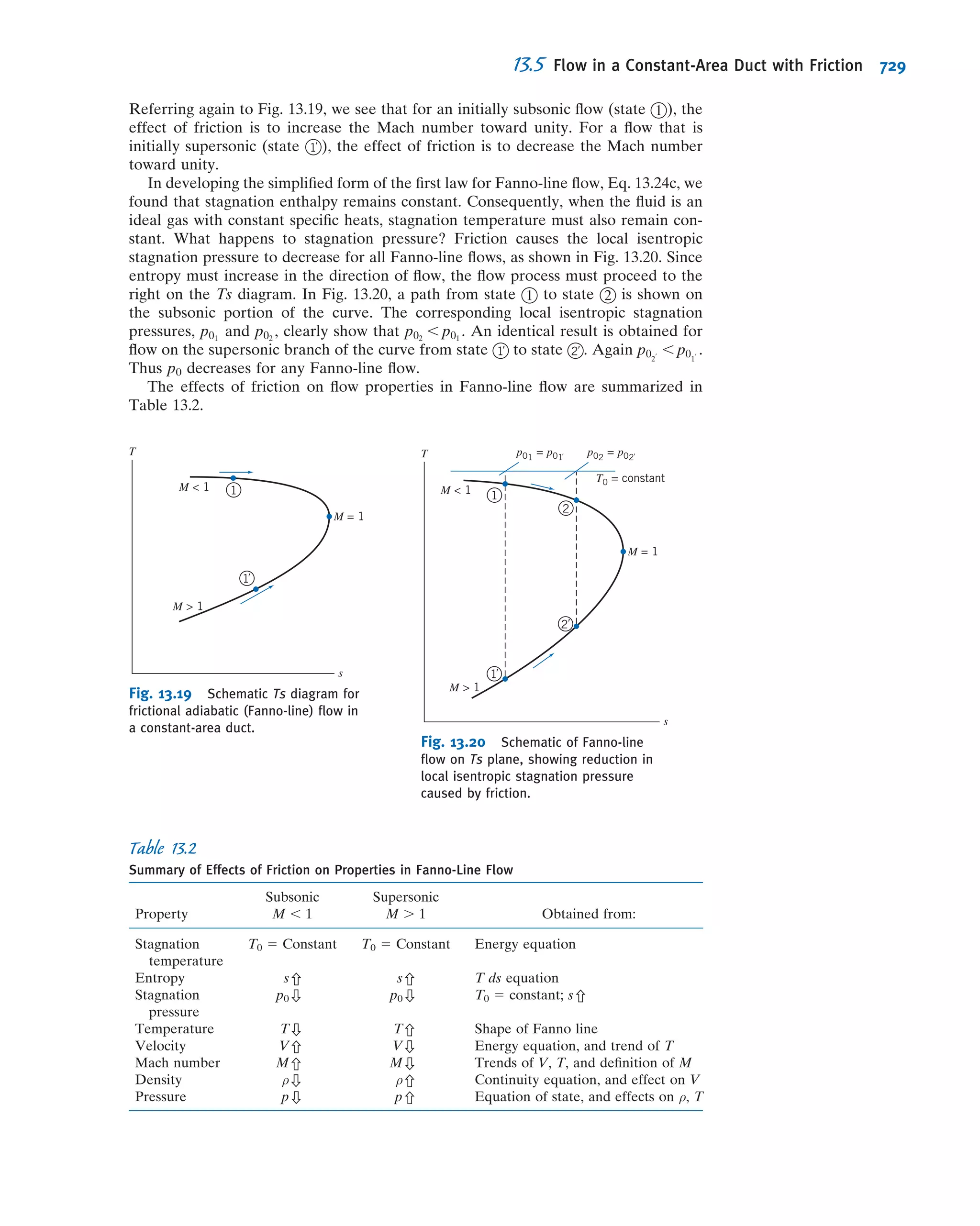

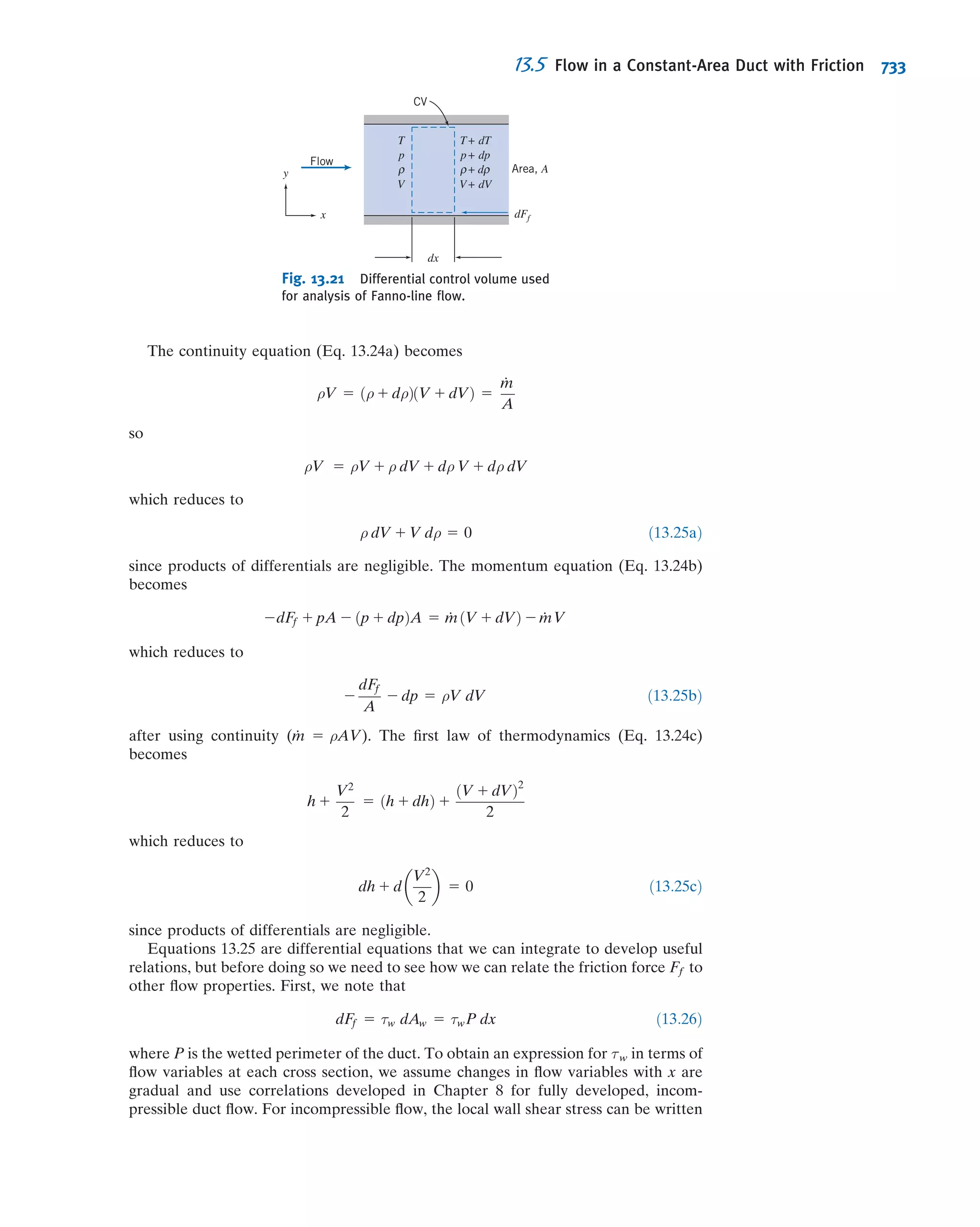


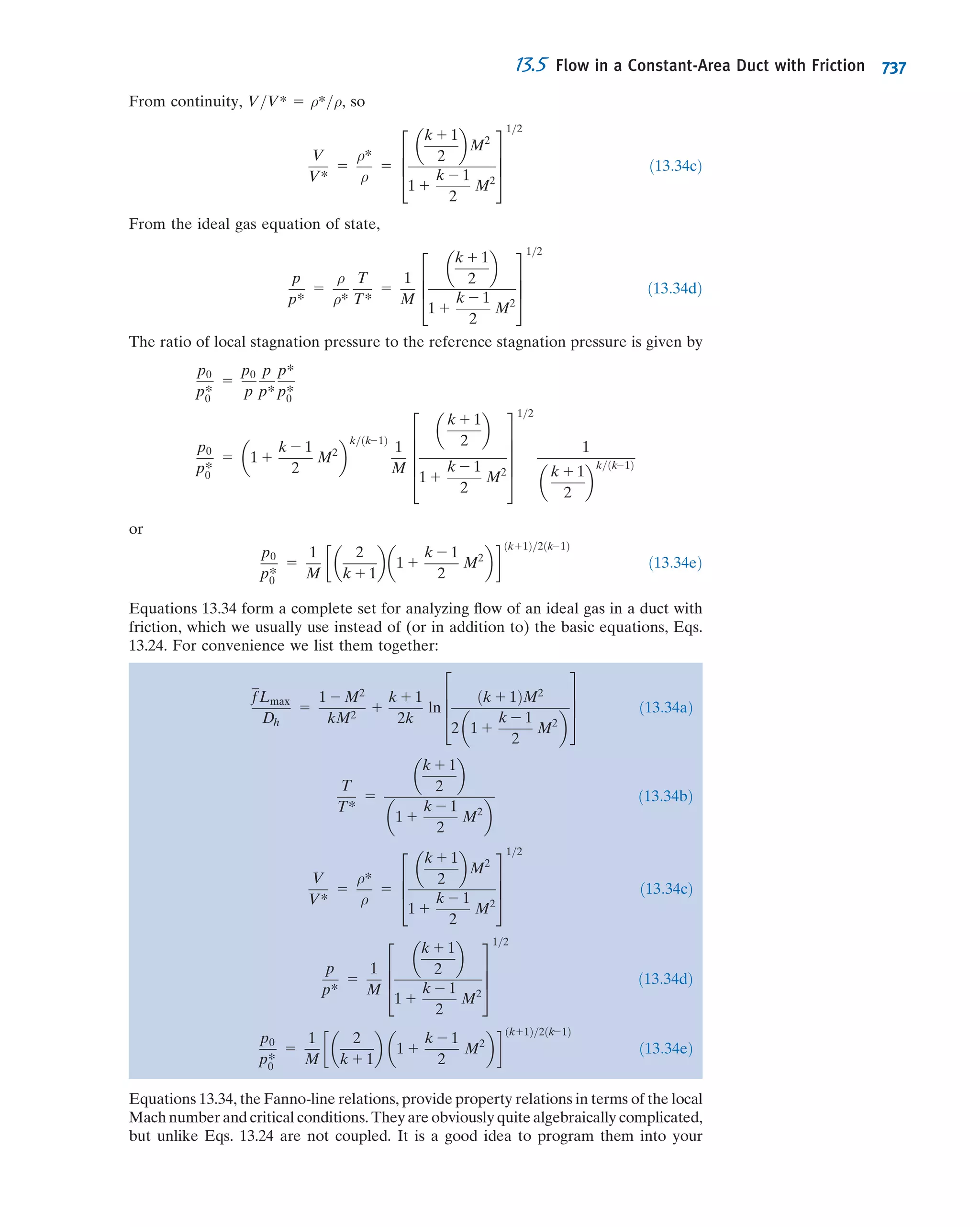


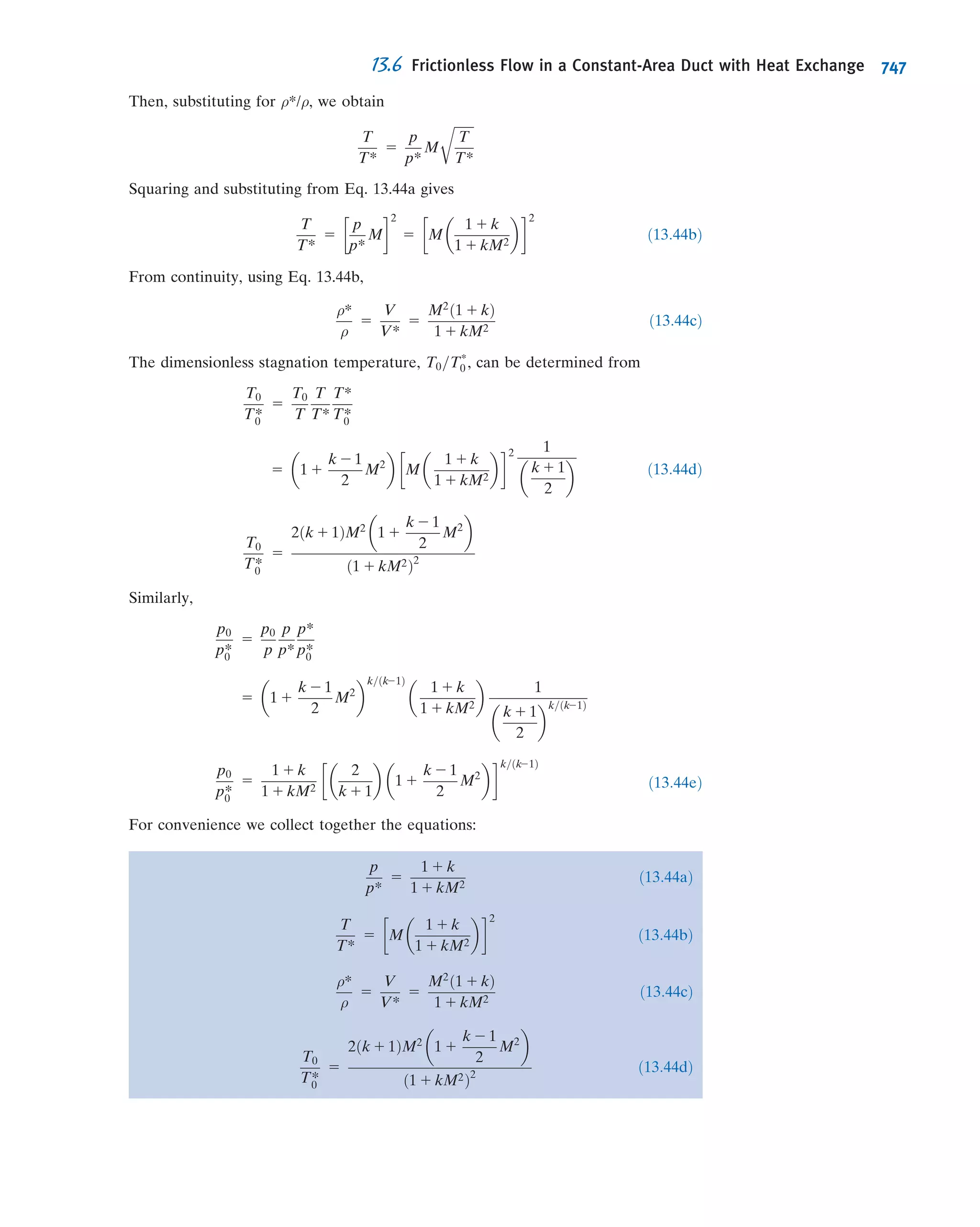


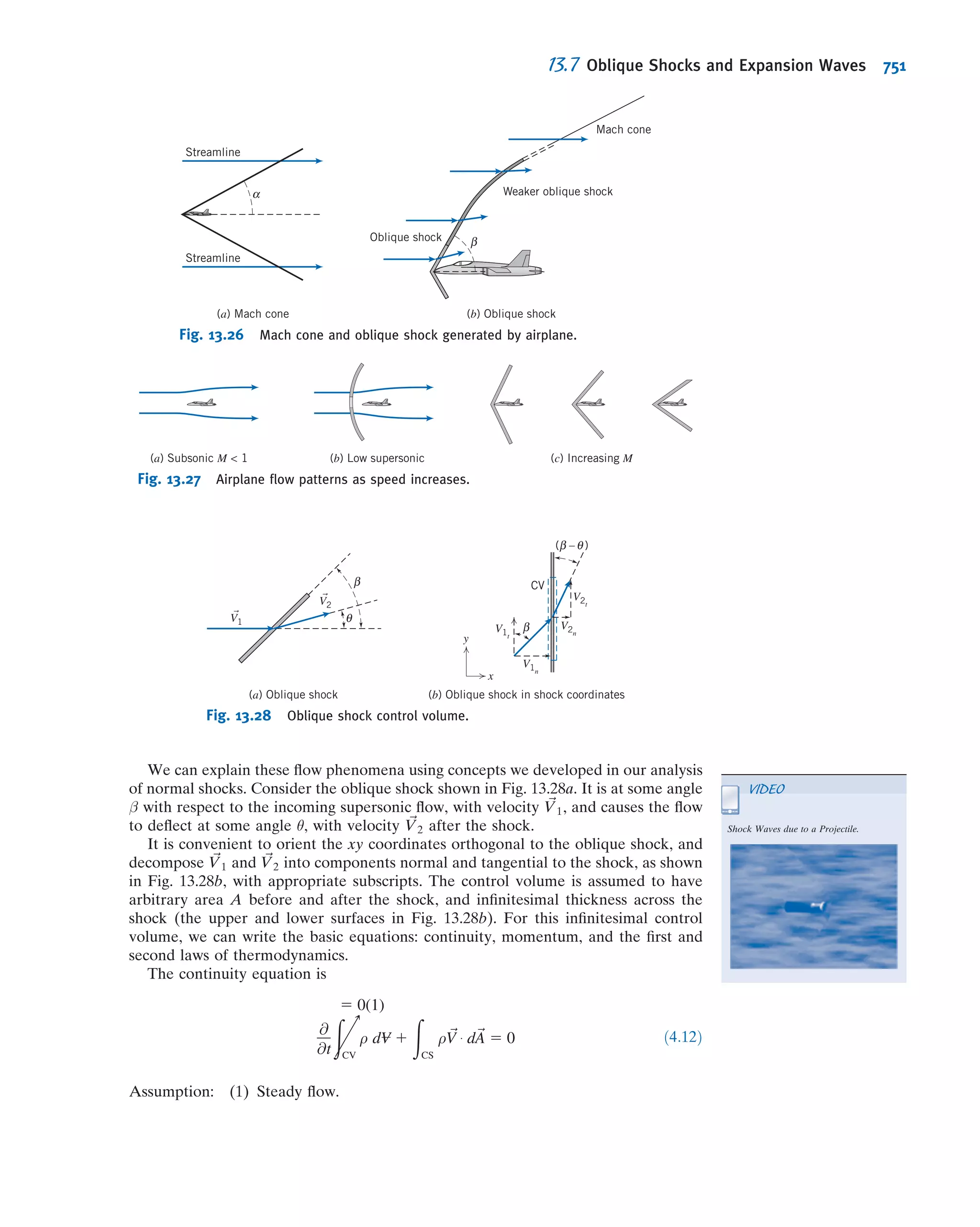
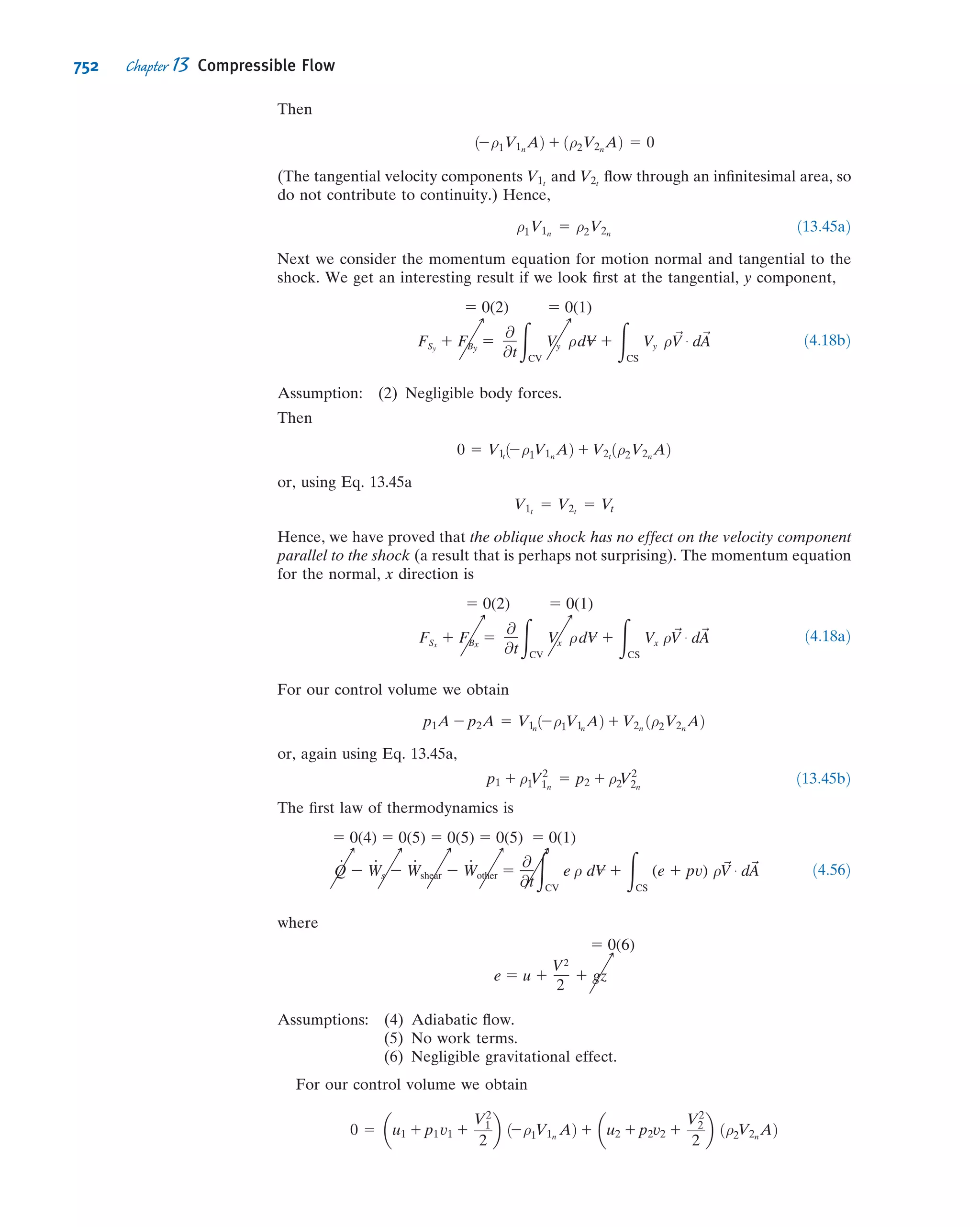

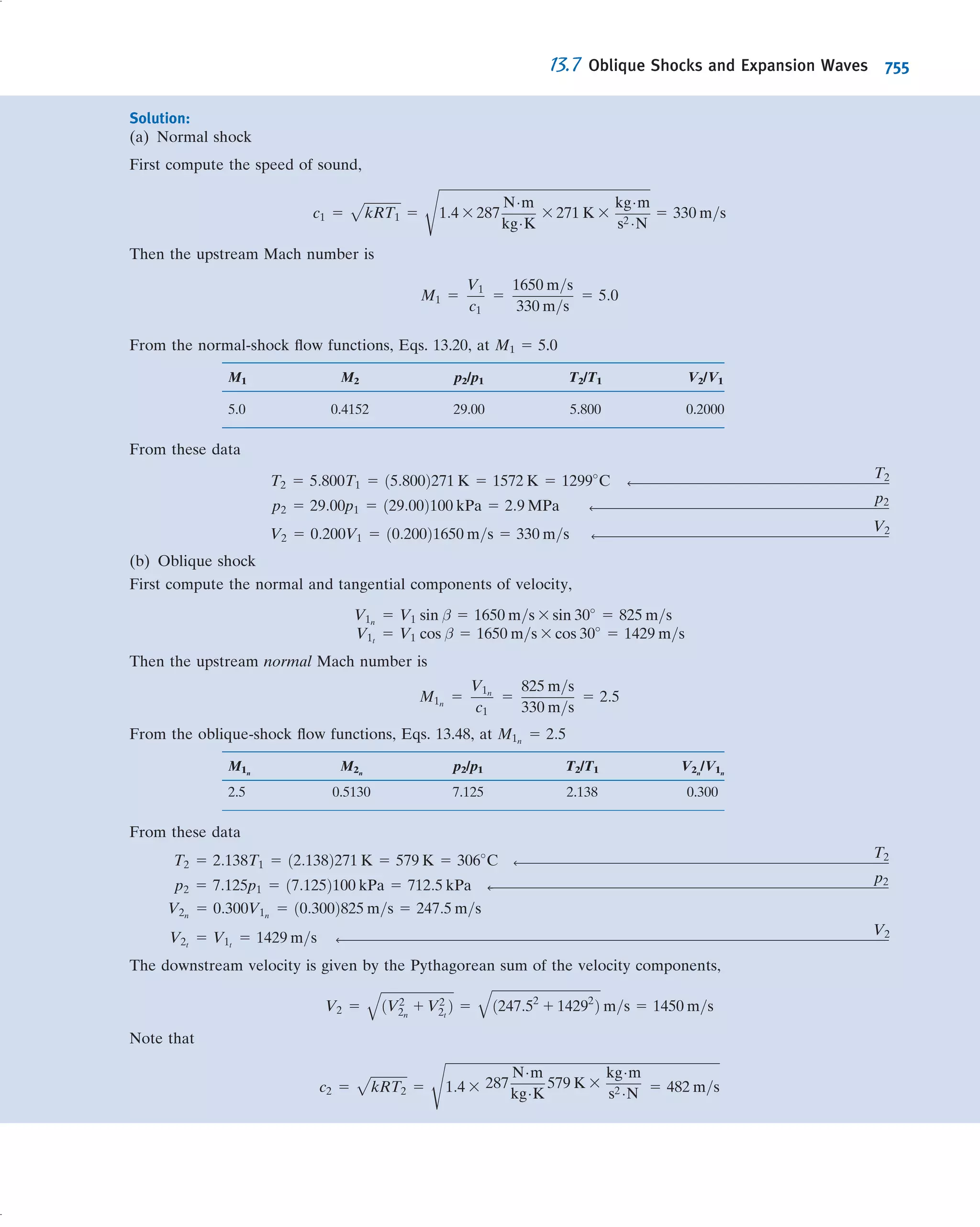
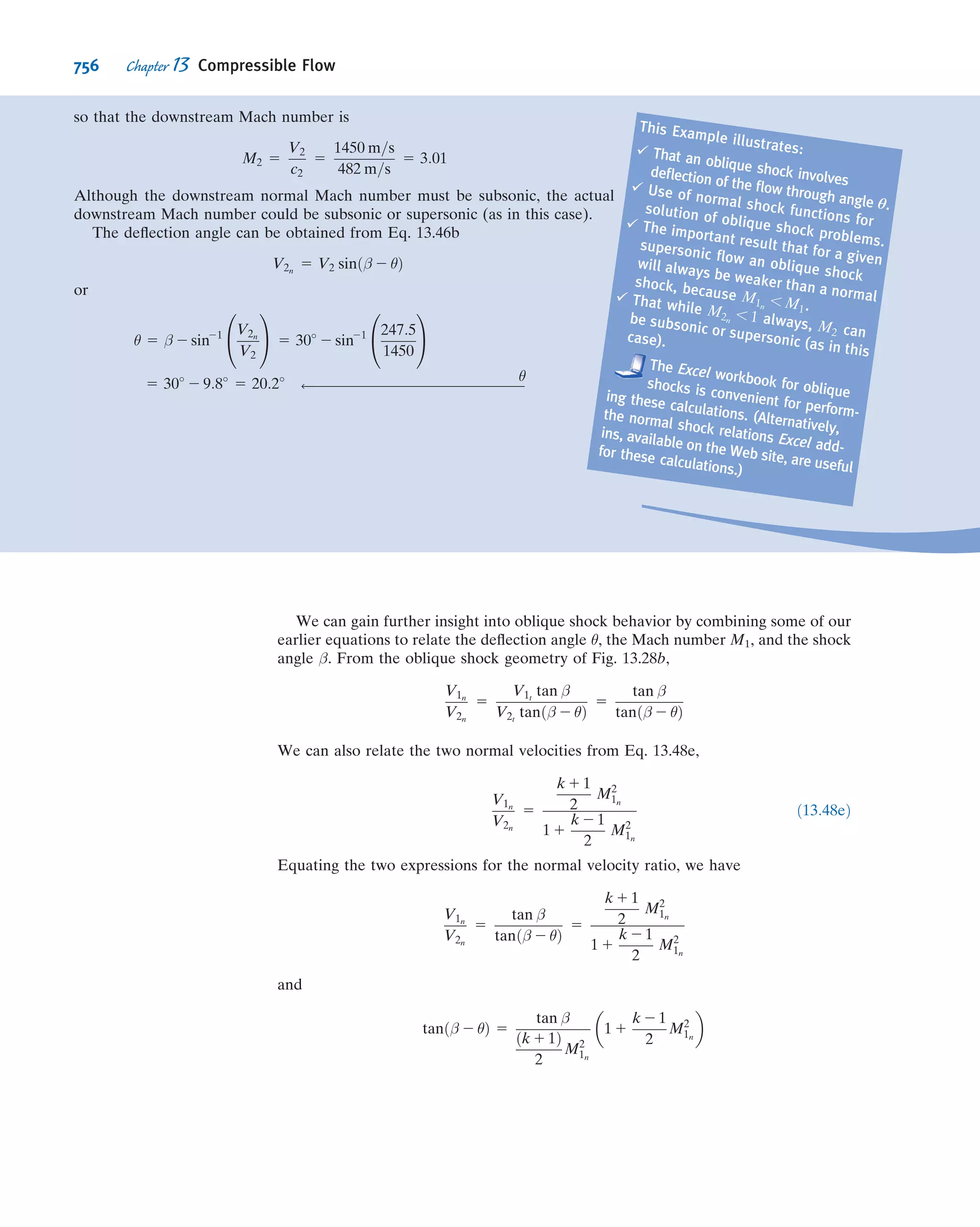

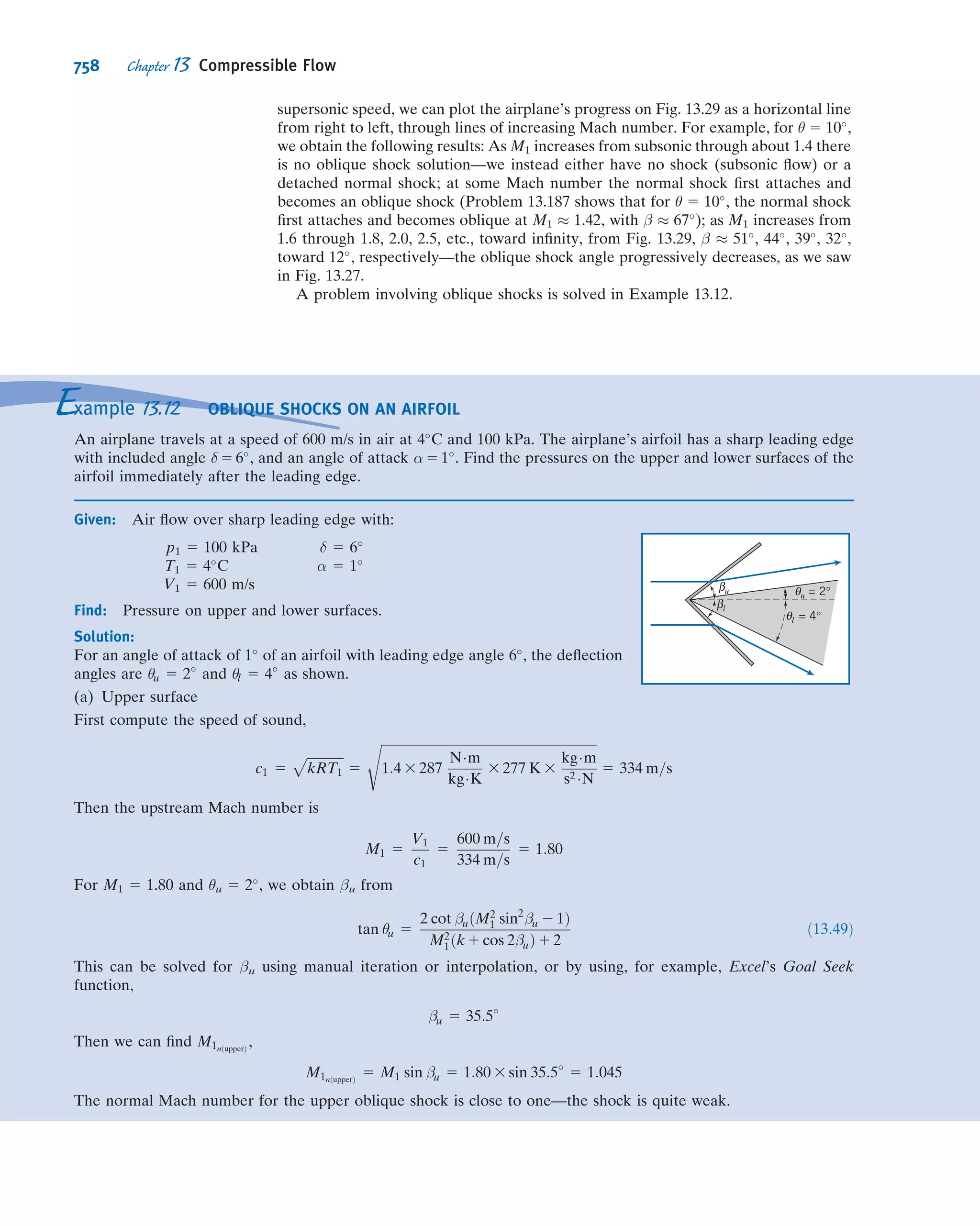
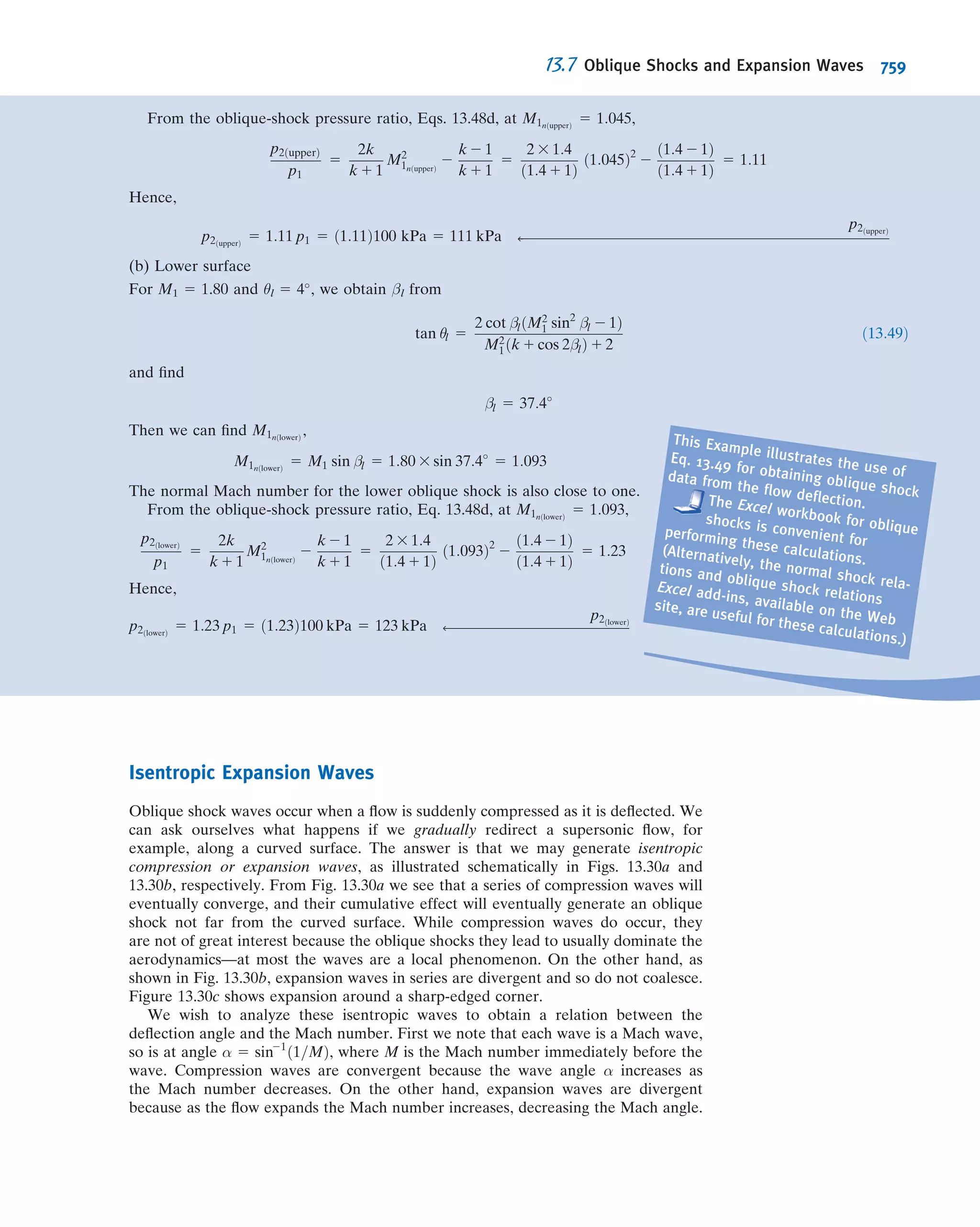

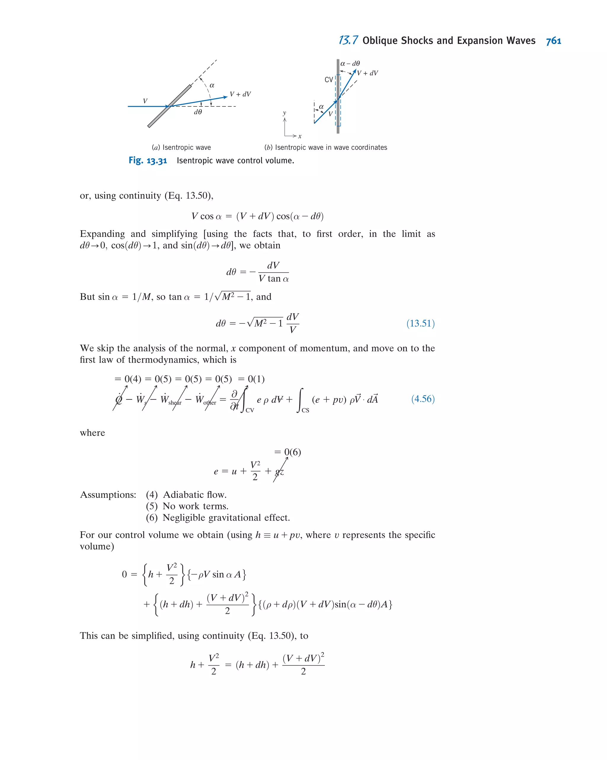


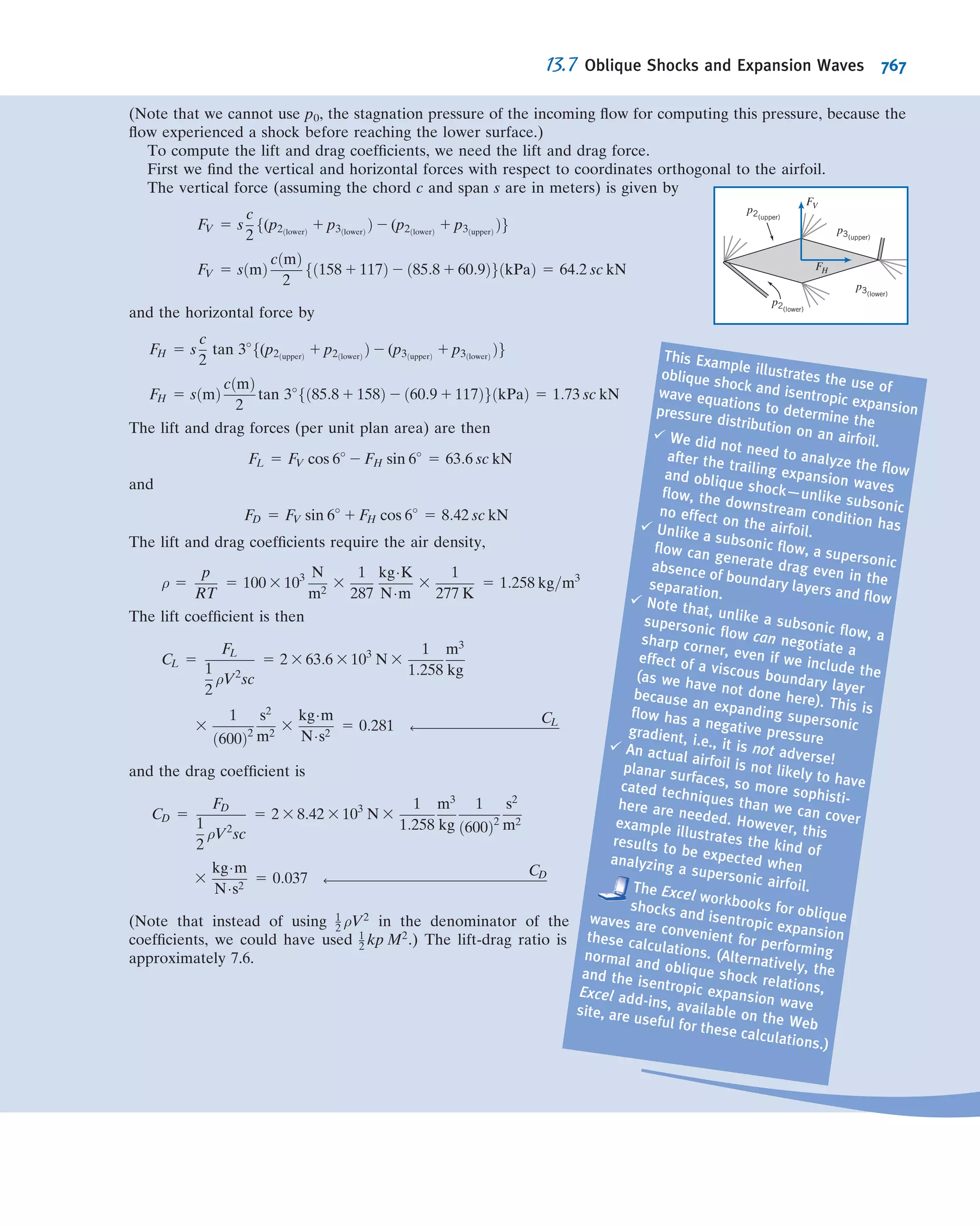

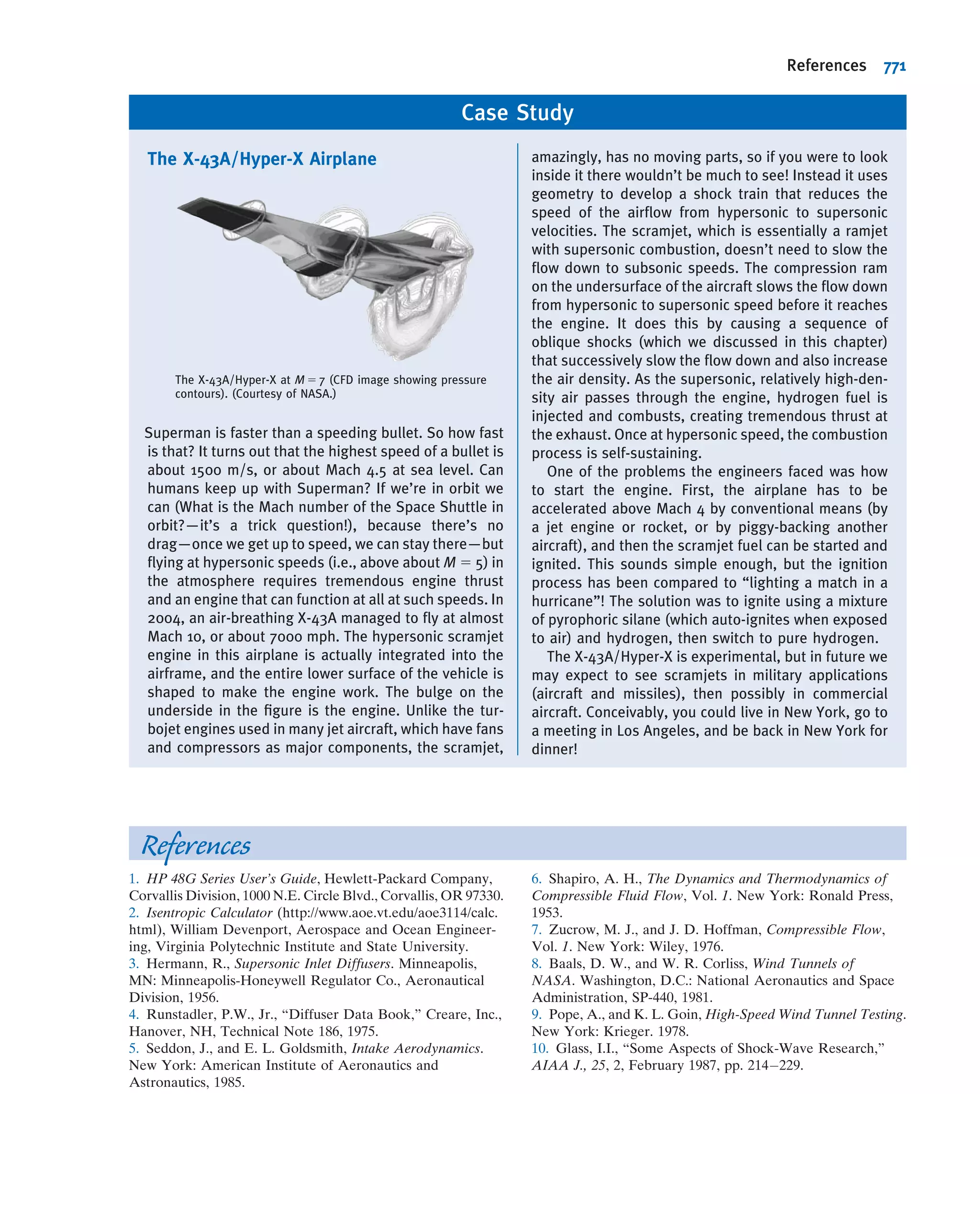


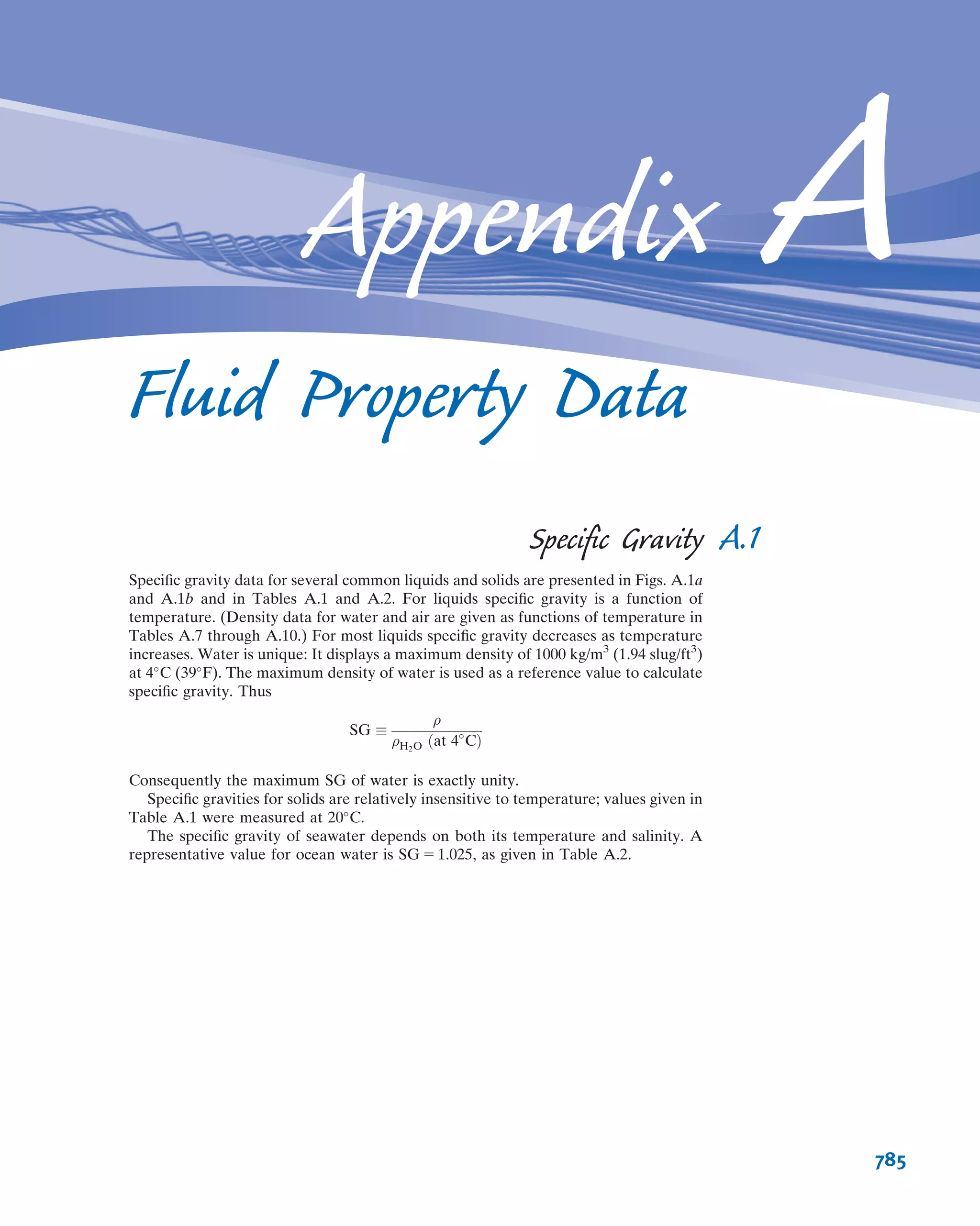
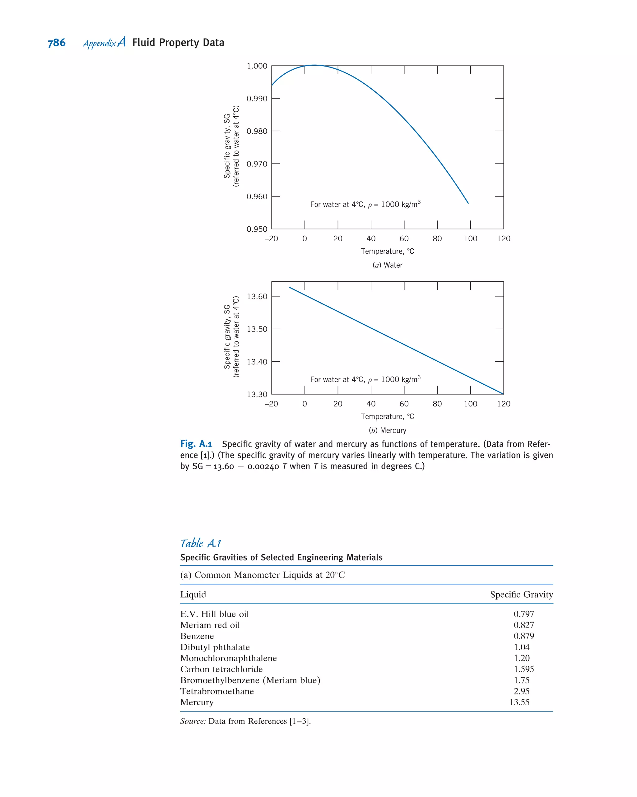
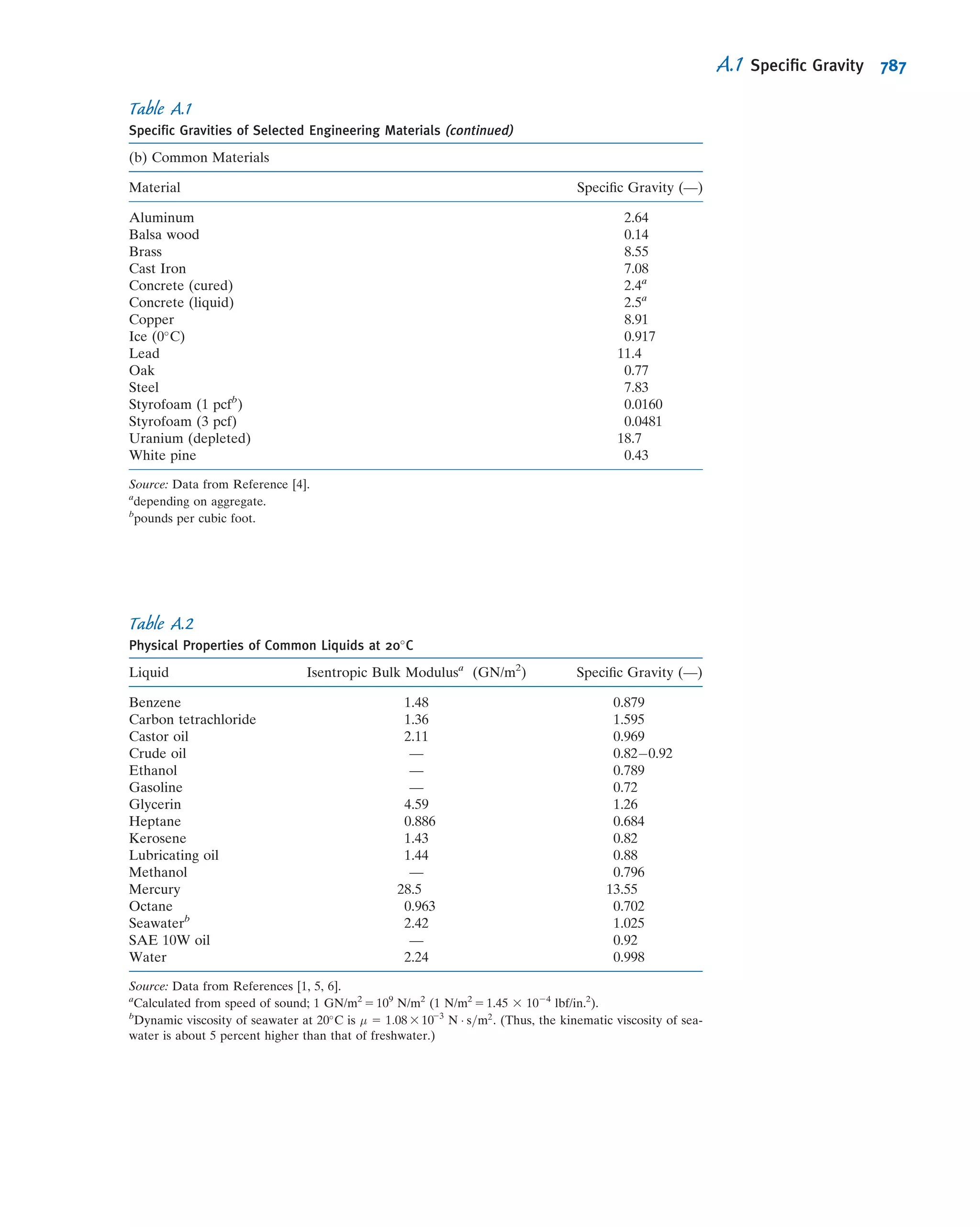

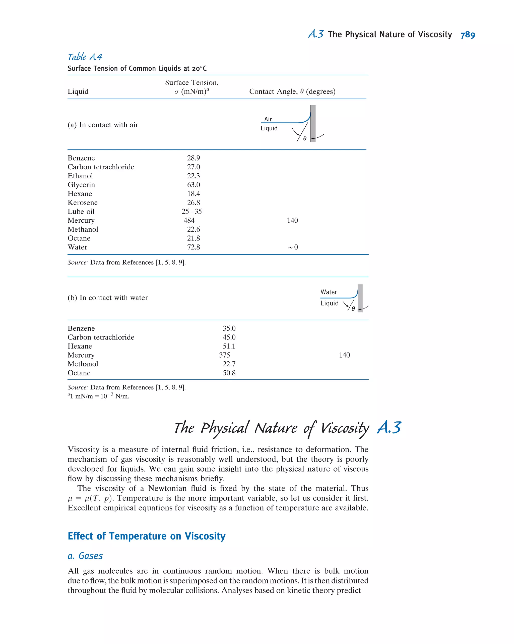


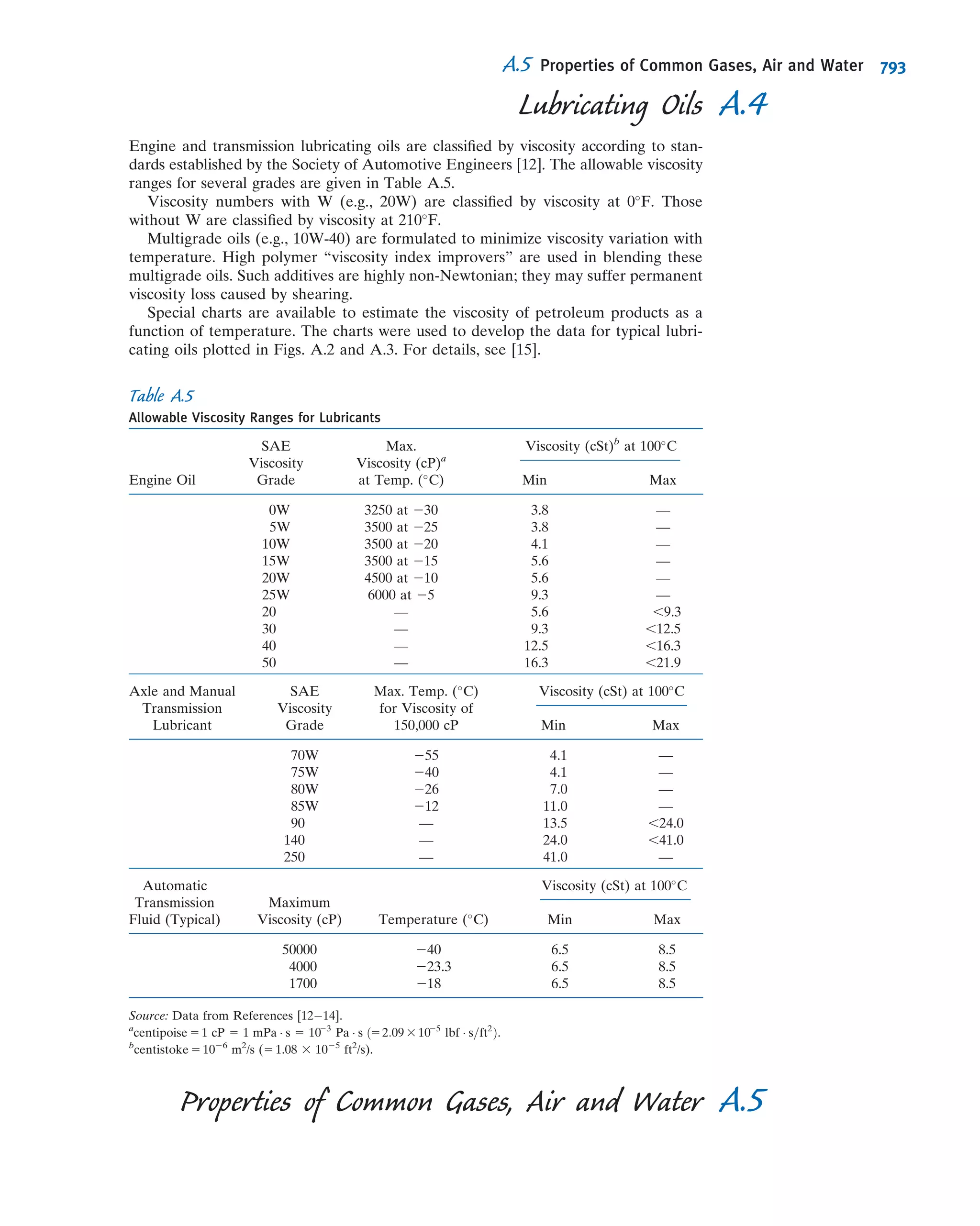


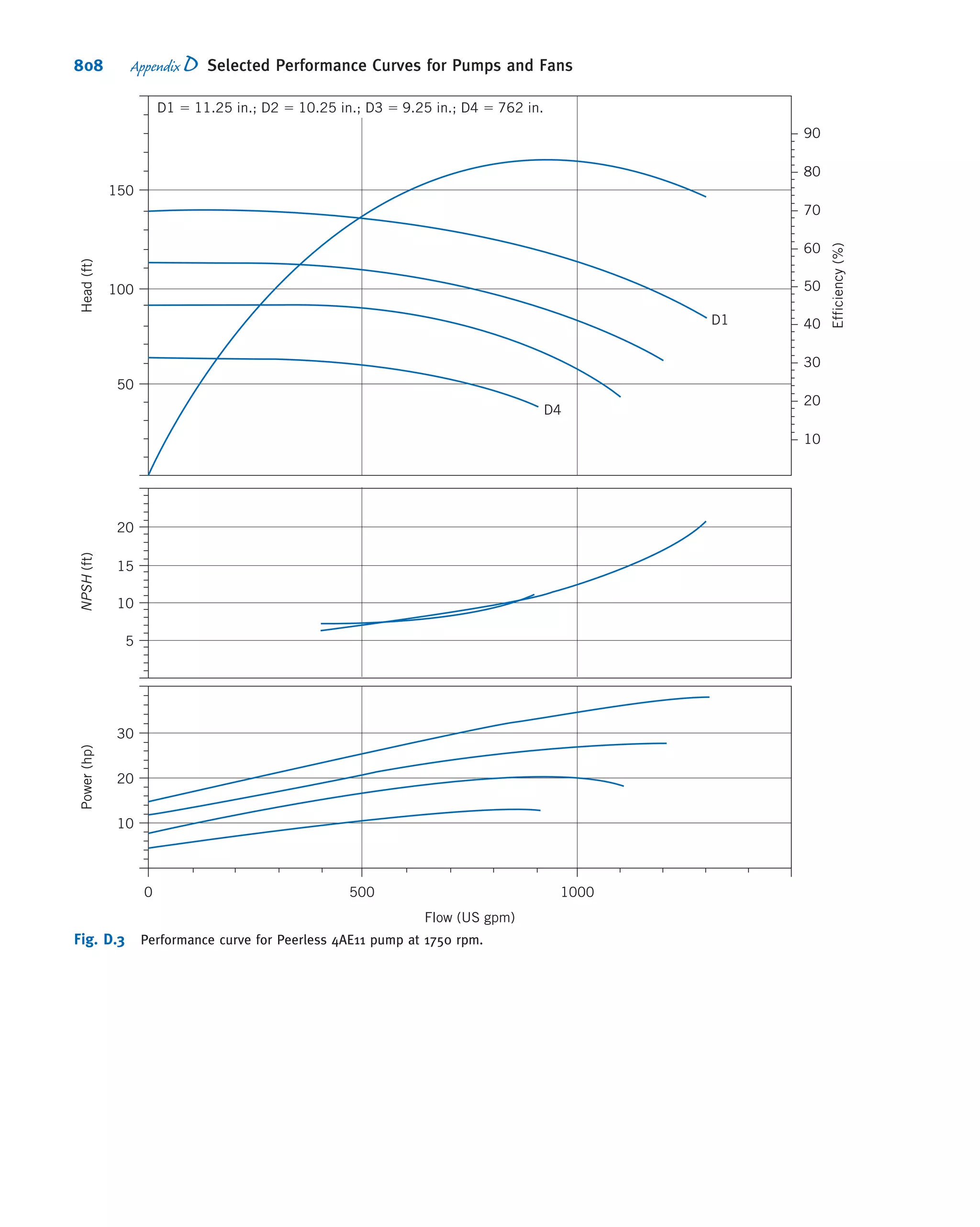
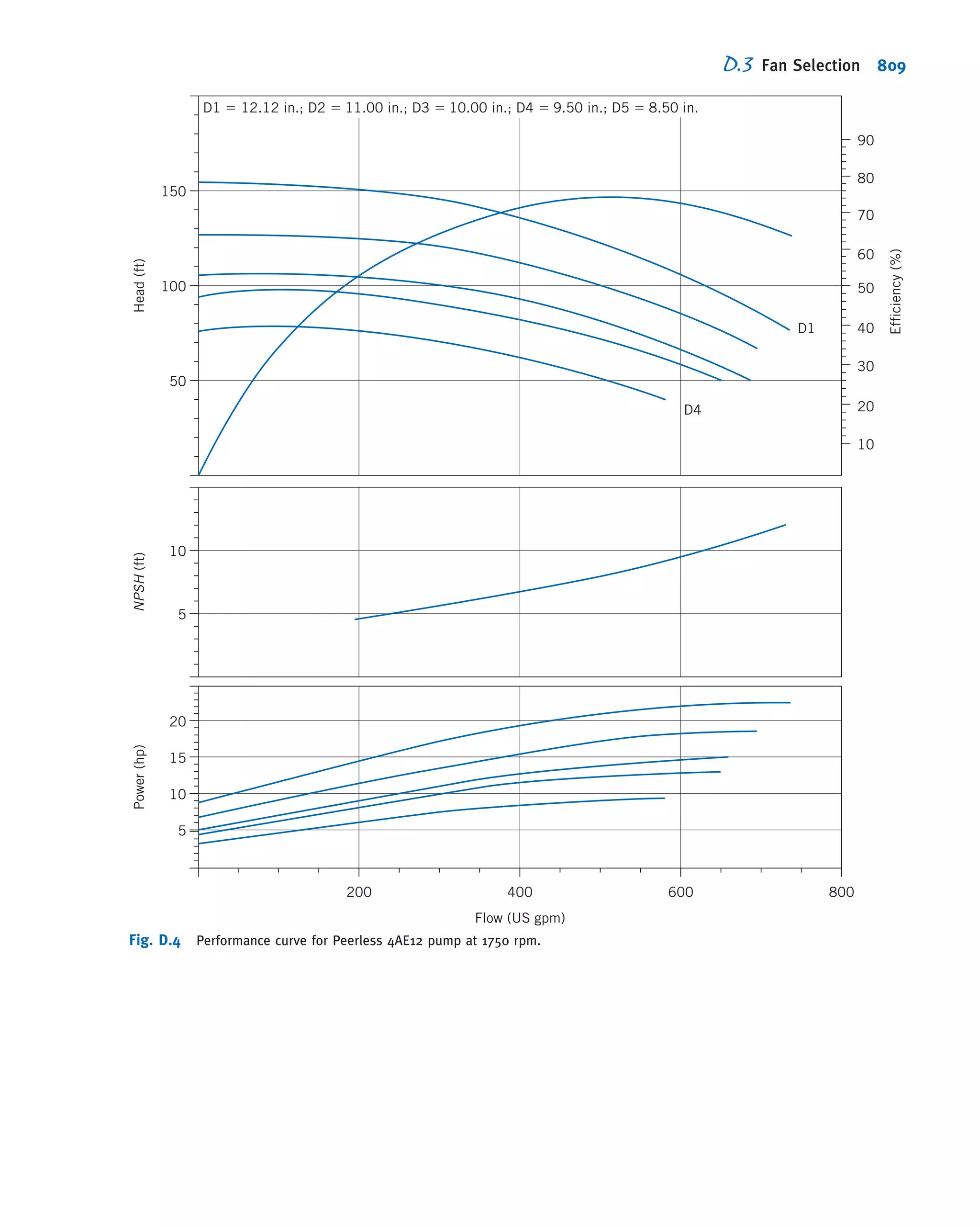

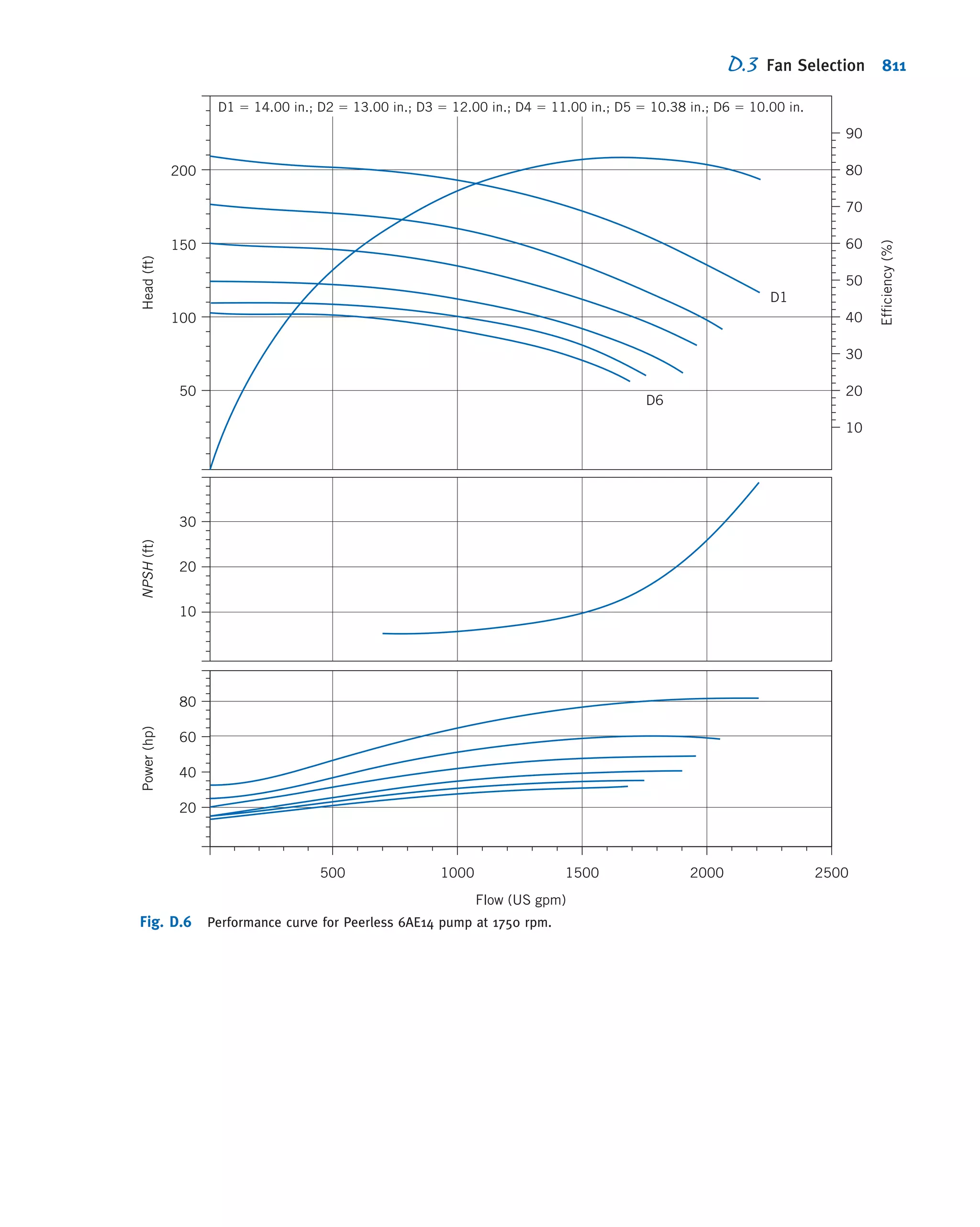
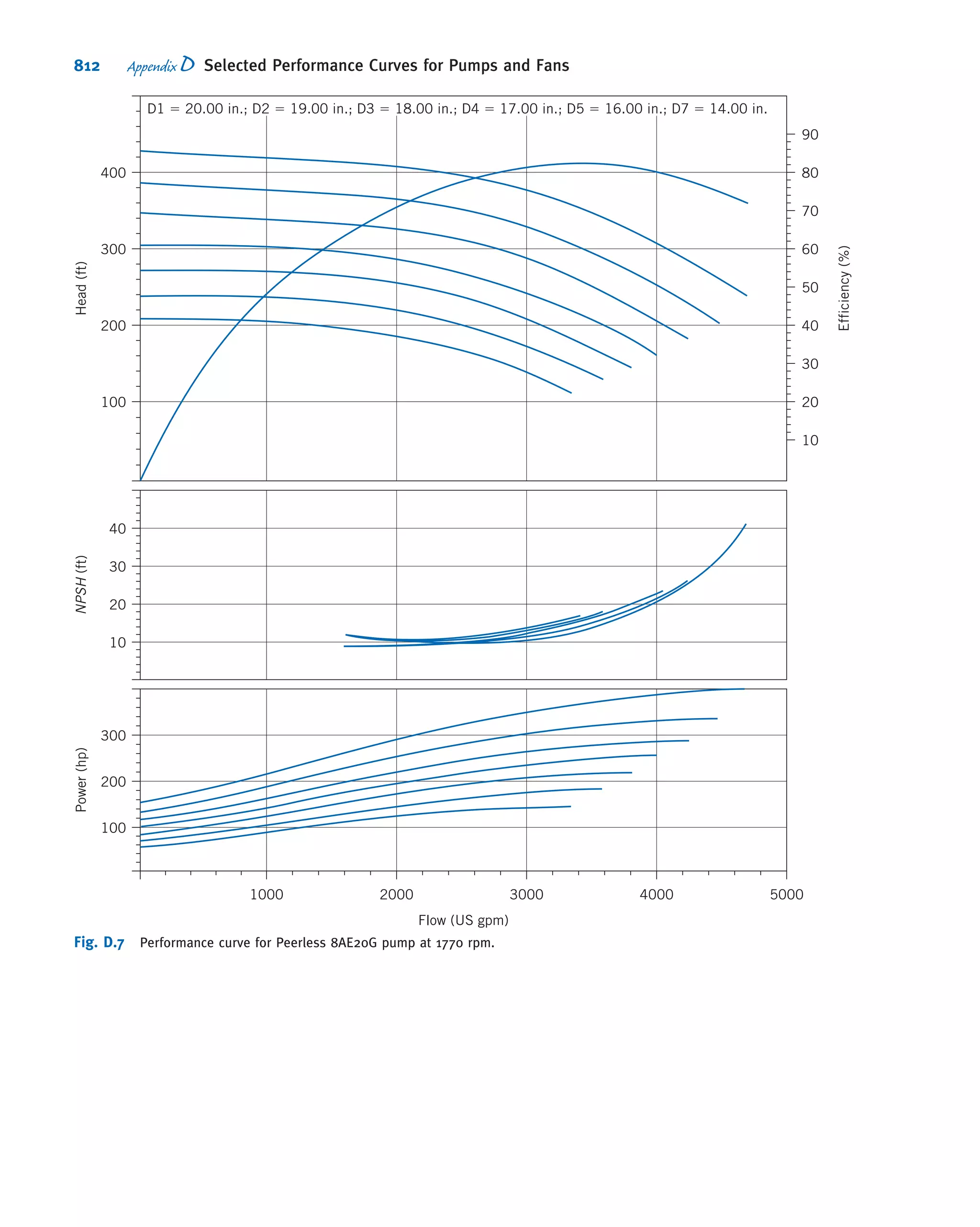

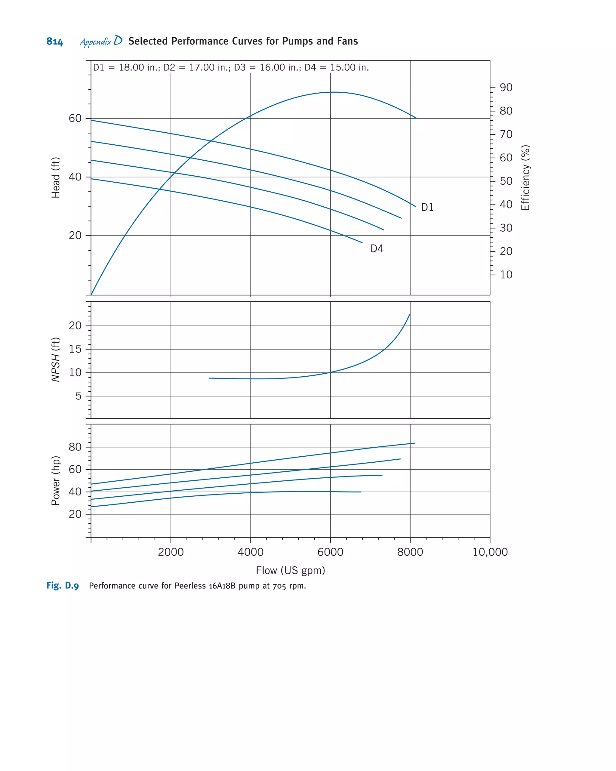


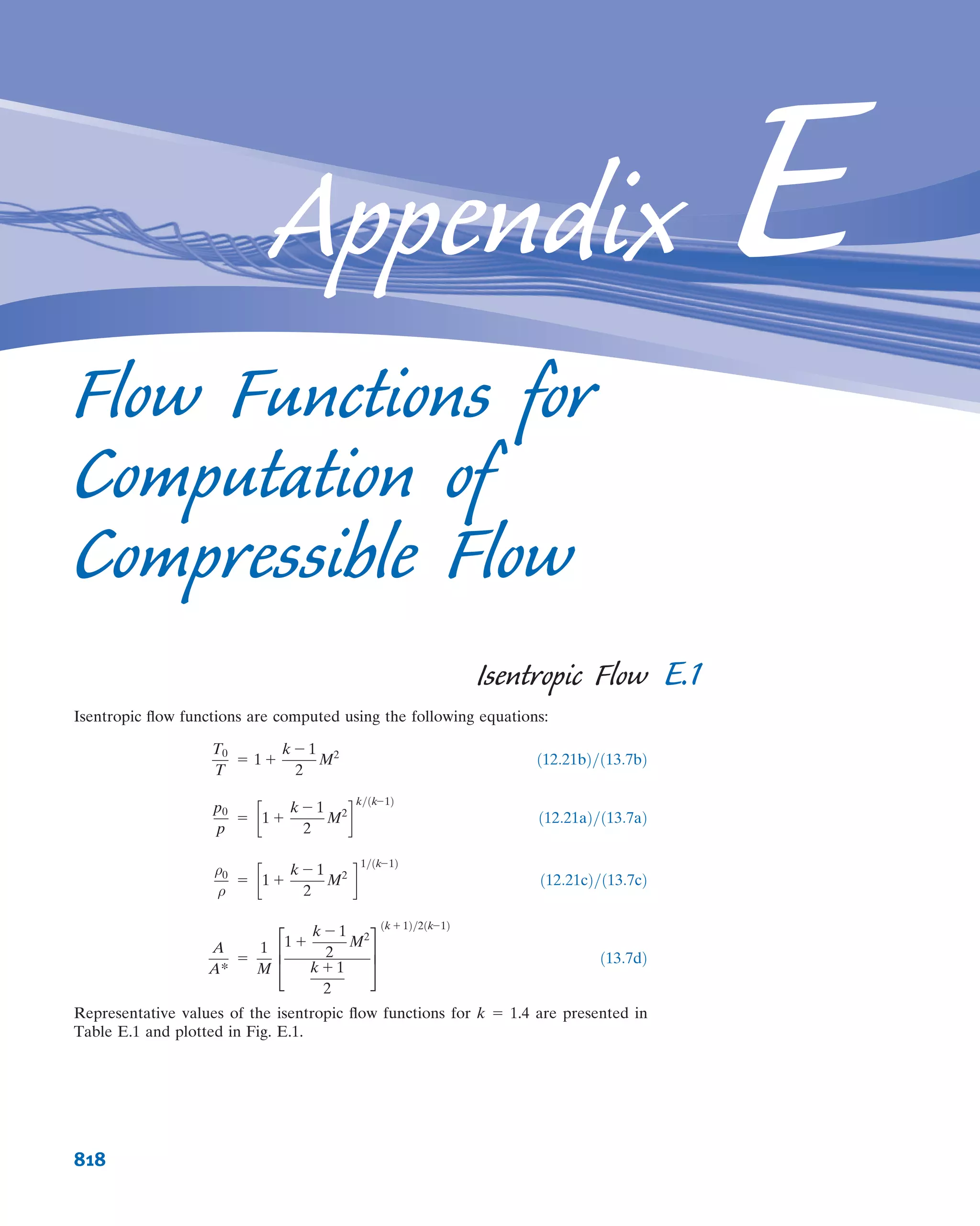
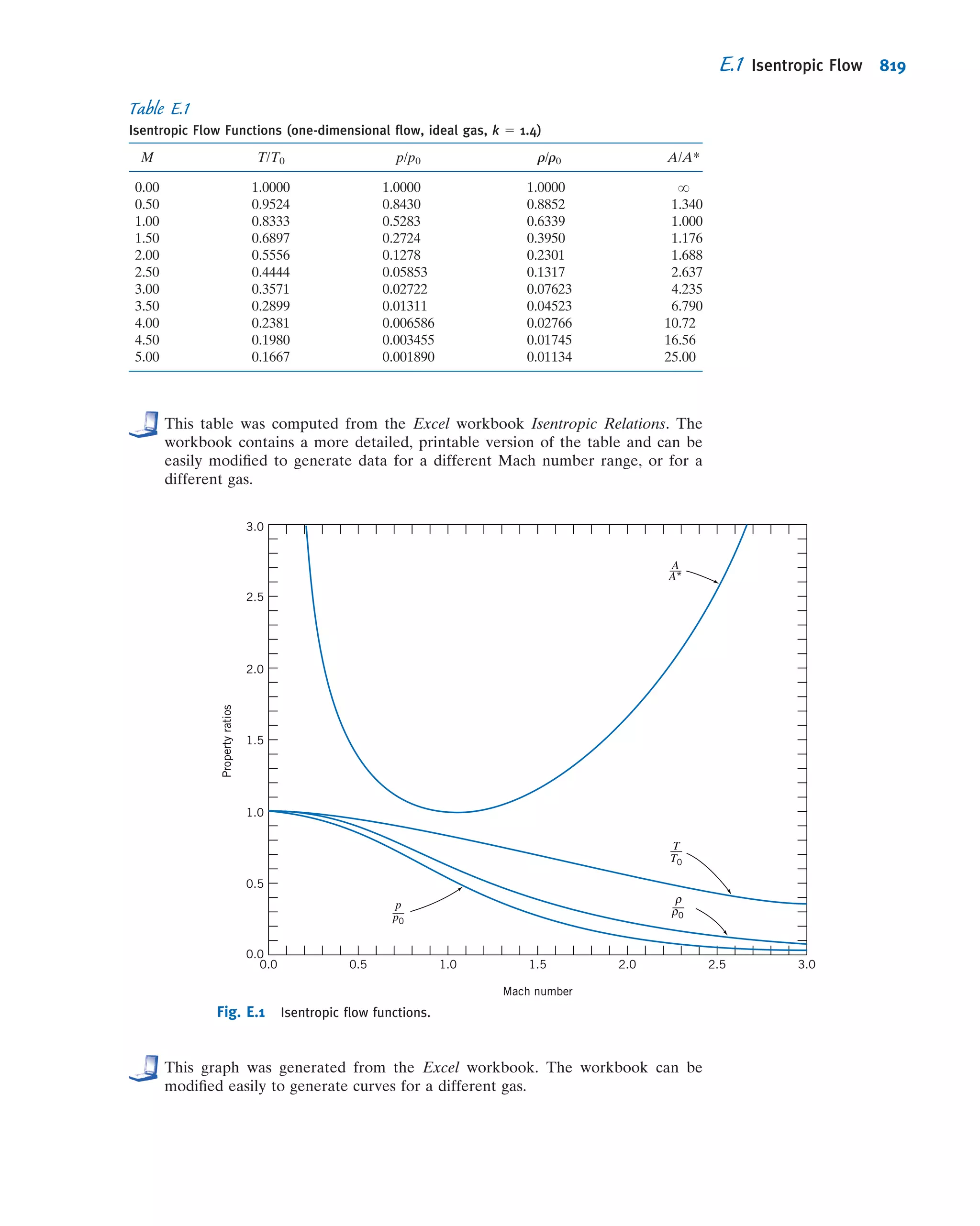
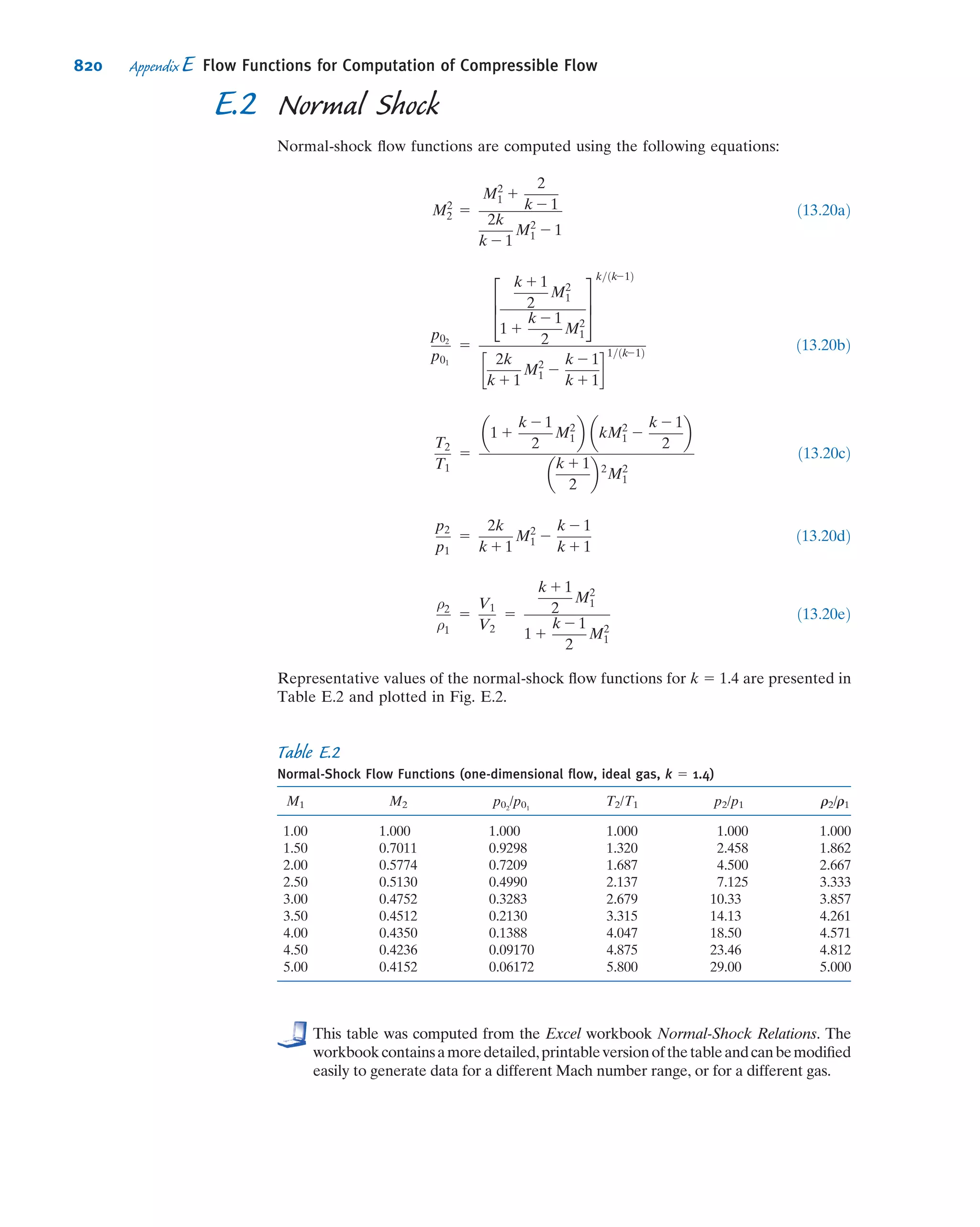


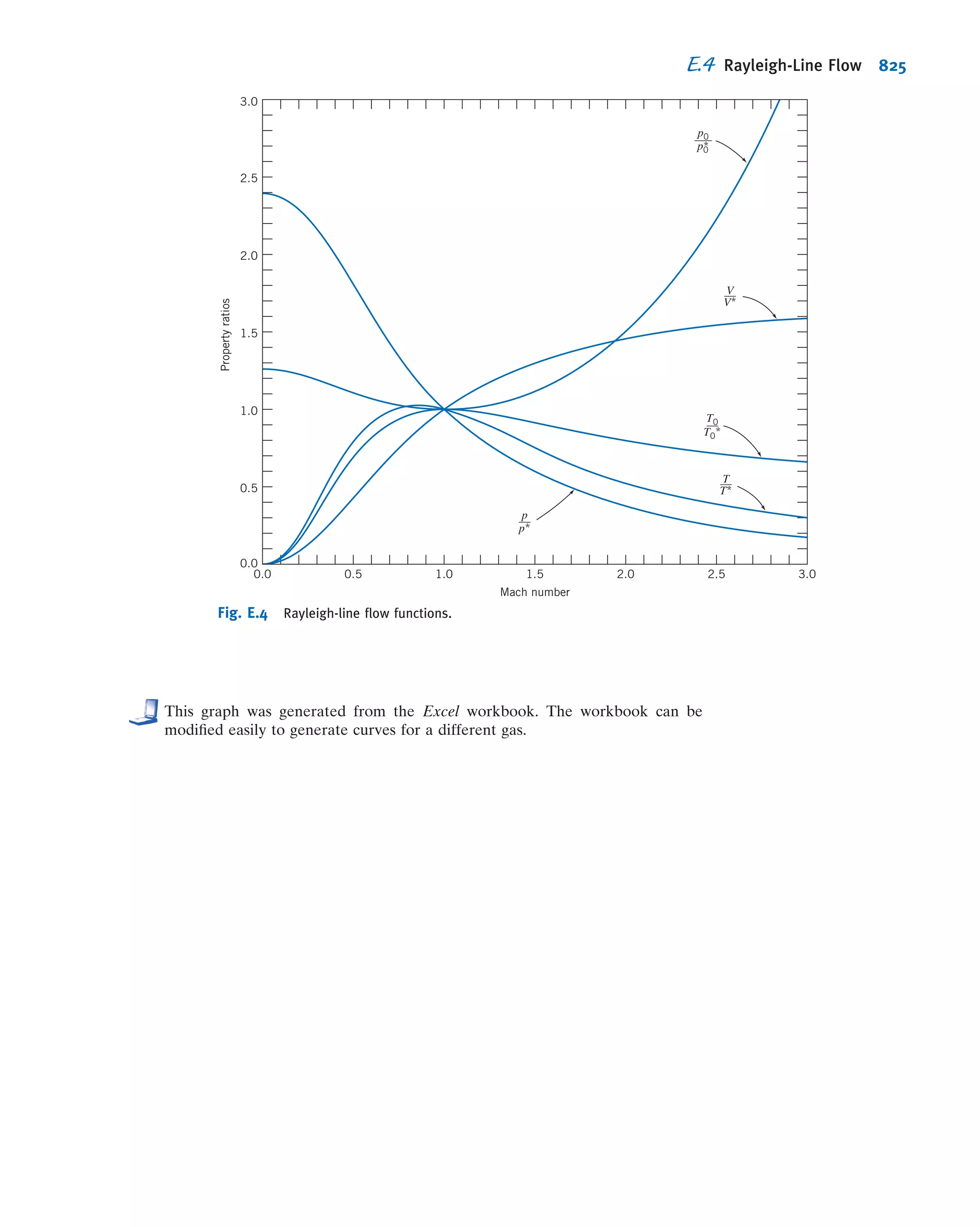


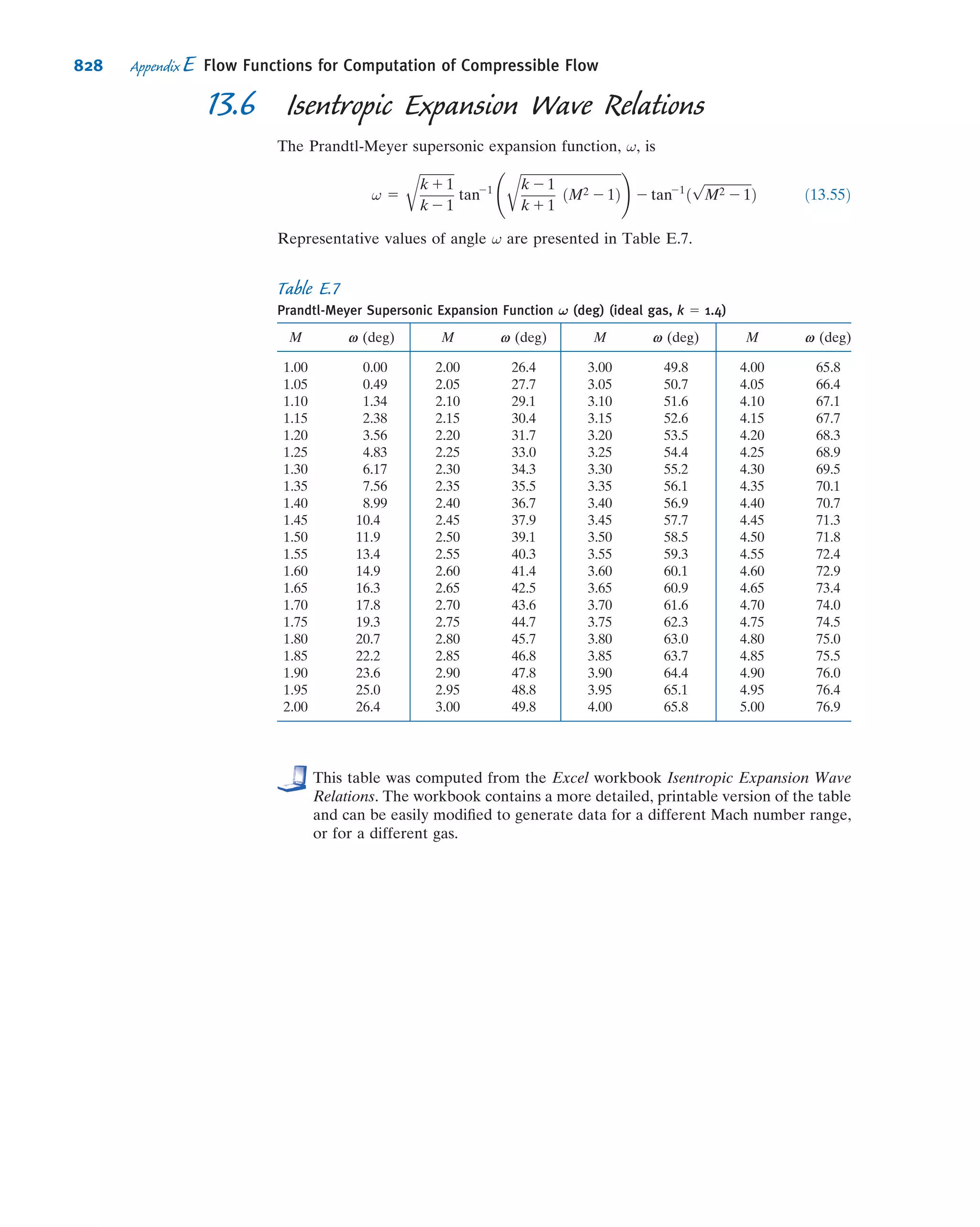


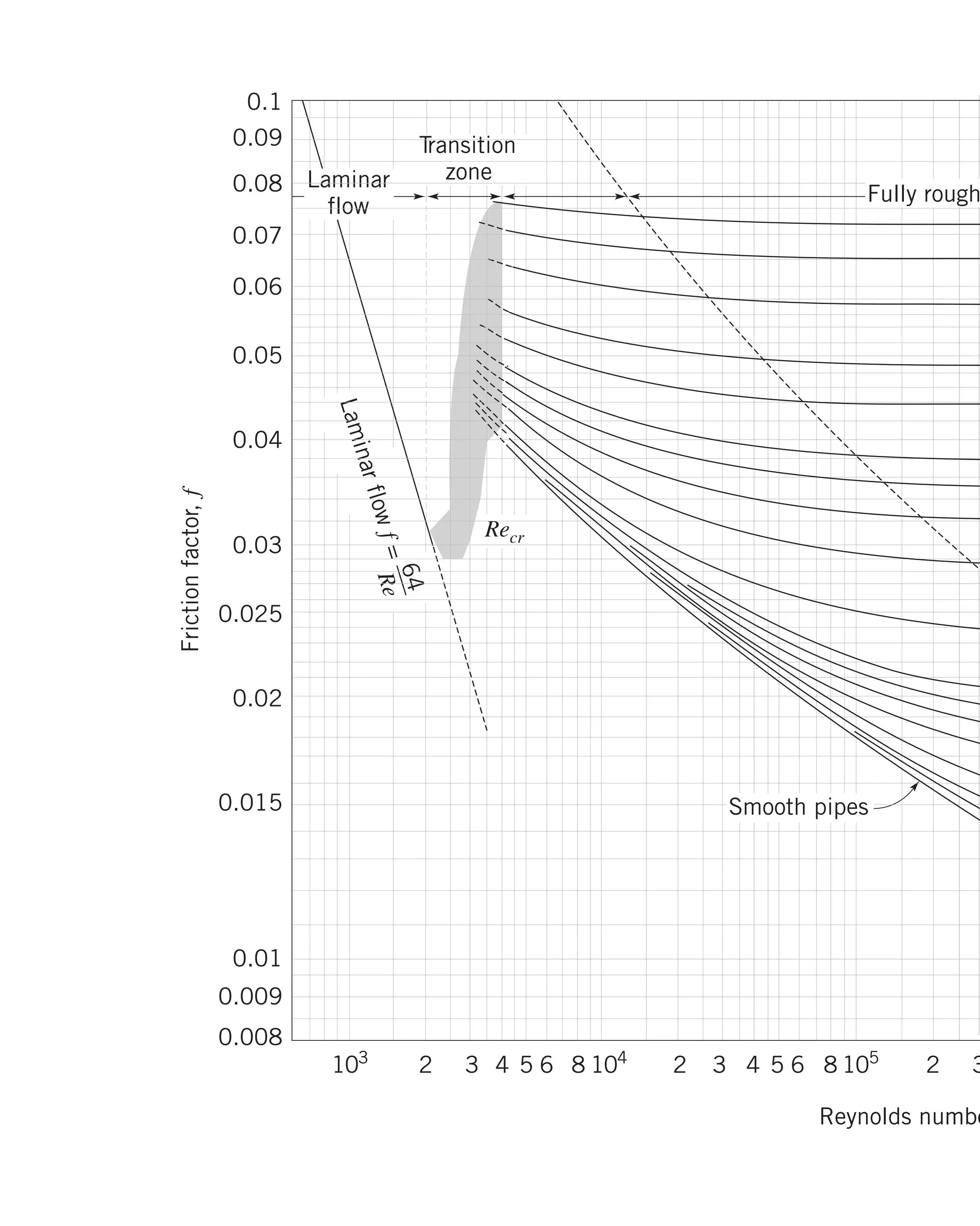


This document provides an overview and summary of WileyPLUS, an online learning environment for teaching and learning. It motivates students with feedback and tracks their progress. It also supports instructors with resources to reinforce course goals. The document provides information on tutorials, student and technical support, and account managers available to help with implementation.


![[Solution manual] fluid mechanics fox & mcdonald](https://cdn.slidesharecdn.com/ss_thumbnails/solutionmanualfluidmechanicsfoxmcdonaldwww-141204014630-conversion-gate02-thumbnail.jpg?width=640&height=640&fit=bounds)


