This document summarizes research using Echo State Networks (ESN) to model and classify electroencephalography (EEG) signals recorded during mental tasks in brain-computer interfaces (BCI). ESN were trained to forecast EEG signals one step ahead in time using data from 14 participants performing four mental tasks. Separate ESN models for each task act as experts in modeling EEG for that task. Novel EEG data is classified by selecting the label of the model with the lowest forecasting error. Offline experiments show ESN can model EEG with errors as low as 3% and classify two tasks with up to 95% accuracy and four tasks with up to 65% accuracy at two-second intervals.

1. Computer Science
Technical Report
Echo State Networks for
Modeling and Classification of EEG Signals
in Mental-Task Brain-Computer Interfaces
Elliott M. Forney, Charles W. Anderson, William J. Gavin,
Patricia L. Davies, Marla C. Roll, Brittany K. Taylor
November 17, 2015
Colorado State University Technical Report CS-15-102
Computer Science Department
Colorado State University
Fort Collins, CO 80523-1873
Phone: (970) 491-5792 Fax: (970) 491-2466
WWW: http://www.cs.colostate.edu

2. Abstract
Constructing non-invasive Brain-Computer Interfaces (BCI) that are practical for
use in assistive technology has proven to be a challenging problem. We assert that
classification algorithms that are capable of capturing sophisticated spatiotemporal
patterns in Electroencephalography (EEG) signals are necessary in order for BCI to
deliver fluid and reliable control. Since Echo State Networks (ESN) have been shown
to be exceptional at modeling non-linear time-series, we believe that they are well-
suited for this role. Accordingly, we explore the ability of ESN to model and classify
EEG recorded during several mental tasks. ESN are first trained to model EEG by
forecasting the signals a single step ahead in time. We then take a generative ap-
proach to classification where a separate ESN models sample EEG recorded during
each mental task. This yields a number of ESN that can be viewed as experts at
modeling EEG associated with each task. Novel EEG data are classified by selecting
the label corresponding to the model that produces the lowest forecasting error. An
offline analysis was conducted using eight-channel EEG recorded from nine partic-
ipants with no impairments and five participants with severe motor impairments.
These experiments demonstrate that ESN can model EEG well, achieving error rates
as low as 3% of the signal range. We also show that ESN can be used to discriminate
between various mental tasks, achieving two-task classification accuracies as high
as 95% and four-task accuracies as high as 65% at two-second intervals. This work
demonstrates that ESN are capable of modeling intricate patterns in EEG and that
the proposed classification algorithm is a promising candidate for use in BCI.
1 Introduction
Brain-Computer Interfaces (BCI) are emerging technologies that allow people to interact with
computerized devices using only changes in mental state [1]. While BCI may eventually lead to
many new forms of human-computer interaction, an important and immediately useful appli-
cation is the development of assistive devices. Since those with limited motor function may find
it difficult to interact through physical movement, BCI may be a useful alternative to mechan-
ical input devices. For those with severe motor impairments that are progressive in nature, all
other forms of assistive technology, such as eye trackers, switches and voice recognition, may
eventually become ineffective. In these cases, even a BCI with a relatively slow communication
rate may prove to be an invaluable tool and, potentially, a person’s only method of communica-
tion [2,3].
Among the approaches that have been proposed for constructing BCI, those that utilize scalp-
recorded Electroencephalography (EEG) appear to be particularly promising [4,5]. Since EEG is
non-invasive, users are not required to undergo surgical procedures and researchers are free to
investigate new methods with minimal risk. Although EEG suffers from a low signal-to-noise
ratio and moderate spatial resolution, its high temporal resolution and history of successful use
in BCI are redeeming [4–6]. Furthermore, EEG hardware is relatively inexpensive and can be
contained in a portable system. Overall, it appears that EEG is well-suited for use in many types
of BCI.
In a number of studies, EEG-based BCI that combine mental-task communication paradigms
with techniques from machine learning have shown considerable potential [7–24]. When using
a mental-task communication paradigm, a user issues instructions to the BCI by performing one
of several predetermined mental tasks. For example, a user might imagine making a fist in order
1

3. to move a cursor to the left or silently sing a song to move it to the right. Mental-task commu-
nication paradigms allow tasks involving visualization, language, analytical thinking, music and
motor imagery to be combined in a way that is user-friendly while also eliciting diverse changes
in EEG across various brain regions [7,18,25,26]. When combined with machine learning, these
BCI may have the potential to attain several degrees of control and a high level of adaptability
on the part of the user as well as the BCI.
Nevertheless, constructing practical BCI that use EEG and mental-task paradigms has proven
to be a challenging problem for several reasons. First, the sheer complexity of the human brain
suggests that EEG signals likely contain sophisticated spatiotemporal patterns. Second, there
does not appear to be any single type of change in EEG that can universally be used to discrim-
inate between mental tasks. Third, the patterns in EEG that are associated with mental tasks
can vary considerably among different BCI users and over the course of time. Finally, the noisy
nature of EEG and the fact that humans are continually performing multiple simultaneous tasks
means that desirable signal components are often masked by noise, artifacts and background
mental activity. We assert that carefully designed machine learning algorithms and signal pro-
cessing techniques are required in order to overcome these challenges and develop BCI that are
capable of delivering reliable and fluid control at a rapid pace.
A number of machine learning algorithms have been proposed for filling this role. For in-
stance, Millán, et al. [20–22], Galán, et al. [23], and Zhiwei, et al. [24], have explored the use
of frequency-domain signal representations constructed from Fourier and Wavelet Transforms
in combination with various classifiers and feature selection algorithms. Although frequency-
domain representations may be well-suited for capturing periodic patterns in EEG, they often
suffer from a limited ability to capture non-stationary and short-term patterns. These methods
also do not typically consider spatial patterns in the form of phase differences across channels.
Approaches proposed by Anderson, et al. [10–13], and Friedrich, et al. [18,19], combine time-
delay embedding with various classifiers and linear transforms for dimensionality reduction.
Time-delay embedding is capable of capturing spatiotemporal patterns; however, the length of
temporal information is limited by the size of the embedding dimension and a large embedding
dimension can lead to a high-dimensional feature space. Although linear transforms and source
separation techniques appear promising for dimensionality reduction, selecting desirable com-
ponents can be challenging and automated techniques have not been adequately explored [27].
An alternative to these approaches that may be able to capture spatiotemporal patterns while
avoiding high-dimensionality involves the use of predictive models. Along these lines, Keirn and
Aunon [7] as well as Anderson, et al. [8, 9], have applied several types of classifiers to the coef-
ficients resulting from linear Autoregressive (AR) models. Subsequently, Coyle, et al. [14], sug-
gested that applying a classifier to the residuals from forecasting models that utilize non-linear
feedforward networks and time-delay embedding may outperform linear AR models. Coyle, et
al. [28–32], have also proposed several other methods that use predictive models to filter and
derive features for BCI.
In our previous work, we have begun to explore the use of errors resulting from forecasting
EEG with Recurrent Neural Networks (RNN), i.e., networks with feedback connections [15–17].
Since RNN can model non-linear processes and because they have an intrinsic state and mem-
ory, we believe that they may be better-suited for modeling EEG than linear AR models and
feedforward networks.
In the present study, we extend our work by exploring the ability of Echo State Networks
(ESN) to model and classify EEG within the framework of mental-task BCI. ESN are a type of RNN
that rely on a large, sparsely connected reservoir of artificial neurons that are tuned only during
the initialization process. A linear readout layer is then trained to map the reservoir activations
2

4. to outputs using a straightforward linear regression. This optimization scheme allows ESN to
be trained quickly, making them suitable for use in interactive BCI. Furthermore, several recent
studies have demonstrated that ESN perform favorably on a number of non-linear dynamical
systems modeling and control problems [33–35].
In order to exploit the apparent potential for ESN to capture patterns in EEG, we propose a
generative classifier. In this approach, ESN are first trained to model EEG by forecasting the sig-
nal a single step ahead in time. Separate models are trained over sample EEG recorded during
each of several mental tasks. Each ESN can be thought of as an expert at modeling EEG associ-
ated with a given mental task. These models are then leveraged to label novel EEG by applying
each ESN to the signal and assigning the class label associated with the model that produces the
lowest forecasting error.
In Section 2, we begin by describing the participants, experimental protocol, EEG acquisition
hardware and preprocessing methods used to construct the dataset examined throughout this
manuscript. In Section 3, we continue by giving a thorough description of our rendition of ESN
as well as the methods that we have used to tune the various parameters involved. In Section 4,
we investigate the ability of ESN to forecast EEG signals and examine the relationship between
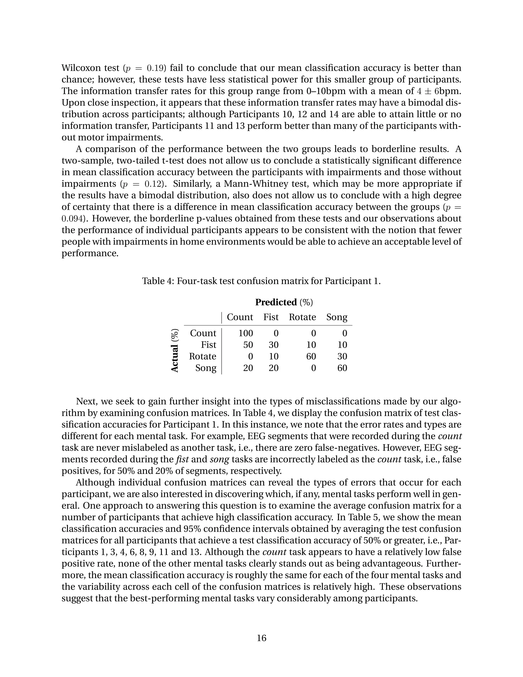
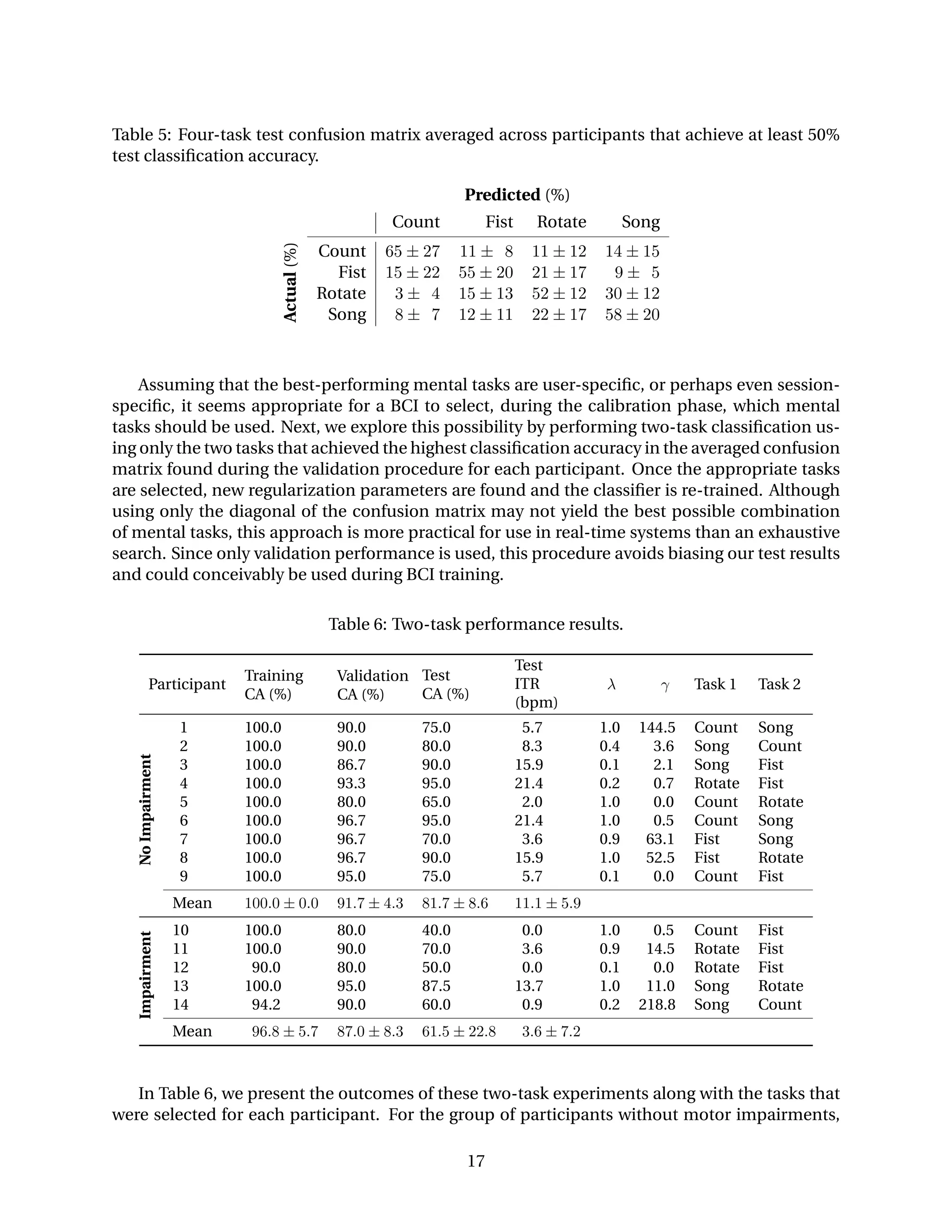
our regularization parameters and the complexity of our models. In Section 5, we formalize our
approach to EEG classification and present the final outcomes of our classification experiments.
Finally, in Section 6, we perform a cursory comparison with other approaches, provide some
concluding remarks and offer potential directions for future research.
2 Participants and Data Collection
In the present study we examine a BCI dataset that we have collected for offline analysis.1 This
dataset was acquired using a g.tec g.MOBILab+ with g.GAMMASys active electrodes. This system
features eight active electrodes that were placed laterally at sites F3, F4, P3, P4, C3, C4, O1 and O2
according to the 10/20 system, depicted in Figure 1. This channel arrangement was designed to
cover a wide variety of cortical regions in each hemisphere of the brain using the eight available
electrodes. The g.MOBILab+ also has an active hardware reference that was linked to the right
earlobe and a passive ground that was placed at site FCz. This system has a sampling frequency
of 256Hz and a hardware bandpass filter from 0.5–100Hz at -3dB attenuation. The g.MOBI-
Lab+ is lightweight, battery-powered and communicates via a bluetooth transceiver. Although
this system offers relatively few channels and a low sampling rate, we believe that its portability
and ease-of-use make it representative of the types of EEG systems that are likely to be used in
practical BCI [36].
Several preprocessing steps were carried out in software in order to reduce noise and arti-
facts. First, a third order, zero-phase Butterworth highpass filter with a cutoff at 4Hz was applied
in order to reduce slow drift and artifacts caused by ocular movement. A stopband filter with
similar characteristics was then applied to the 59–61Hz band in order to eliminate interference
induced by external power mains and equipment. Next, a common-average reference was ap-
plied in order to attenuate signals and interference common to all channels. Finally, each chan-
nel was standardized to have zero mean and unit variance using the sample mean and variance
from the relevant training partition. This standardization procedure ensures that the signals for
each channel have roughly the same scale and prevents the errors produced by our forecasting
models from being dominated by a single channel. A pilot study involving the validation data
for the first five participants supports our use of these preprocessing steps.
1
This dataset is publicly available at http://www.cs.colostate.edu/eeg.
3

5. Figure 1: Eight-channel subset of the 10/20 system used for EEG acquisition. The channels used
are shown in gray.
Data were collected from a total of 14 participants. Nine participants had no known medical
conditions and EEG recording took place in the Brainwaves Research Laboratory in the College
of Health and Human Sciences at Colorado State University [37, 38]. This group is intended to
represent the best-case scenario for a BCI user by minimizing interference from environmen-
tal noise sources and by avoiding other potential challenges that might arise when recording
EEG from those with motor impairments. The remaining five participants had severe motor
impairments, three with progressive multiple sclerosis and two with quadriplegia due to high-
level spinal cord injuries. For this group, EEG recording took place in each participant’s home
environment in order to closely replicate realistic operating conditions for an assistive BCI.
Table 1: Mental tasks used and cues shown to the participants.
Cue Task description
Song Silently sing a favorite song.
Fist Imagine repeatedly making a left-handed fist.
Rotate Visualize a cube rotating in three-dimensions.
Count Silently count backward from 100 by threes.
Following the application of the EEG cap, each participant was positioned comfortably in
front of a computer screen and instructed to perform one of four mental tasks during a visual
cue in the form of a single word, summarized in Table 1. All data collection and cue presentation
was performed using custom software [39]. Participants were asked to perform each task con-
sistently and repeatedly during the cue. They were also asked to move as little as possible and
to blink as infrequently as comfort allowed. Each cue was presented on the screen in a random
order for 10 seconds during which the participant was instructed to perform the correspond-
ing task. A blank screen was then presented for five seconds during which the participant was
instructed to relax. Each participant performed a single practice trial after which they were al-
4

6. lowed to ask the operator questions. After the practice trial, five additional trials were performed
yielding 50 seconds of data per mental task totaling 200 seconds of usable EEG per participant.
Participants 9 and 13 were exceptions to this, having only completed four trials due to a bat-
tery failure and procedural error, respectively. The EEG data were then split into two-second
segments for our classifiers to label, yielding 25 segments per mental task for a total of 100 EEG
segments per participant. Our choice of a two-second interval is supported by our previous re-
search [16], which suggests that assigning class labels at a rate of 0.5–1 instructions-per-second
leads to a high information transfer rate while not exceeding the rate at which a BCI user can be
reasonably expected to send instructions to the system.
The EEG segments for each participant were then divided into a 60% partition for training
and 40% for testing generalization performance. All model tuning and parameter selection was
performed using a five-fold cross validation over the training partition. Final test performance
was evaluated by training the model over the entire training partition using the parameters
found during cross-validation and then observing the performance of the model on the unused
test partition.
3 Echo State Networks
Echo State Networks (ESN) are a type of artificial neural network originally proposed by Herbert
Jaeger and with an international patent held by the Fraunhofer Institute for Intelligent Analy-
sis [33,34,40]. ESN have several properties that may be beneficial for capturing patterns in EEG.
First, ESN have recurrent connections that give them memory and the ability to incorporate
information from previous inputs. This allows ESN to capture temporal patterns without us-
ing frequency-domain representations or explicitly embedding past signal values. Second, ESN
are easily extended to the multivariate case and typically include sigmoidal transfer functions,
allowing them to capture non-linear spatiotemporal relationships. Third, ESN have several pa-
rameters that can be used to limit the complexity of the network. This allows ESN to be regular-
ized in a way that may be robust to noise, artifacts and background mental activity. Finally, ESN
can be trained and evaluated quickly on commodity computing hardware, making real-time ap-
plications feasible.
3.1 Architecture
ESN have a two-layer architecture, depicted in Figure 2. The first layer, termed the reservoir,
consists of artificial neurons with sigmoidal transfer functions. The neurons in the reservoir
have weighted connections from the network inputs as well as weighted recurrent connections
with a single-timestep delay. The second layer, termed the readout, consists of neurons with
feedforward connections and linear transfer functions.
Consider an ESN with L inputs, M reservoir neurons and N outputs. The network inputs can
then be thought of as a multivariate function of time with x(t) denoting an L × 1 column vector
of signal values at time t. The reservoir output, also known as the network context, is then the
M × 1 column vector
z(t) = tanh(H¯x(t) + Rz(t − 1)) (1)
where H is the M × (L + 1) adjacency matrix of feedforward weights into the reservoir and R is
the M × M matrix of recurrent weights. Note that a bar over a matrix denotes that a row of ones
has been appended for a bias term. We choose to use the hyperbolic tangent transfer function,
denoted tanh, because it is symmetrical, fast to compute and commonly used in ESN.
5

7. y1(t) y2(t) y3(t)
x1(t) x2(t) x3(t) Input
Reservoir
Readout
Output
∑ ∑ ∑
H
R
V
Figure 2: The architecture of an Echo State Network with inputs X, input weights H, recurrent
weights R, readout weights V and outputs Y.
The final output of the network at time t is then the N × 1 column vector
y(t) = V¯z(t) (2)
where V is the N × (M + 1) matrix of weights for the readout layer. For the sake of notational
brevity, we write the network output at time t as
y(t) = esn(x(t)). (3)
3.2 Training and Parameter Tuning
The primary difference between ESN and many other types of recurrent networks is that the
reservoir weight matrices, H and R, are not optimized during the training procedure. Instead,
they are chosen in a semi-random fashion that is designed to yield a large number of diverse
reservoir activations while also achieving the Echo State Property (ESP). Briefly stated, a reser-
voir is said to possess the ESP if the effect on the reservoir activations caused by a given in-
put fades as time passes. The ESP also implies that the outputs produced by two identical ESN
will converge toward the same sequence when given the same input sequence, regardless of the
starting network context.
In order to achieve these properties, we follow a modified version of the guidelines suggested
by Jaeger [33]. First, the feedforward weights into the reservoir, H, are chosen to be sparse with
80% of the weights being zero. Sparsity is intended to improve the diversity of the reservoir acti-
vations by reducing the effect of any single input on all of the reservoir neurons. The remaining
weights are selected from the random uniform distribution between −α and α.
Typically, α is chosen empirically through trial and error. We take this a step further by assert-
ing that the value of α should be selected in a way that limits the saturation of the tanh reservoir
transfer function. This is done by taking a sample EEG signal and examining the distribution of
6

8. Figure 3: Histogram of reservoir activations and the hyperbolic tangent for α = 0.35 and λ = 0.6
and N = 1000 for sample EEG. The majority of activations do not lie in the saturated regions of
tanh.
the reservoir activations over the hyperbolic tangent. We illustrate this in Figure 3 by superim-
posing the hyperbolic tangent over a histogram of the reservoir activations generated from the
training EEG for Participant 1 when α = 0.35. In this case, the vast majority of activations lie on
the near-linear and non-linear regions near the center while few activations fall on the saturated
regions at the tails. Although this distribution changes somewhat as other network parameters
vary, we find that a value of α = 0.35 works well in the current setting.
Next, our initial recurrent reservoir weights, R0, are also chosen to be sparse with 99% of the
weights being zero and with the remaining weights selected from a random uniform distribution
between −1 and 1. In order to achieve the ESP, R0 is then scaled to have a spectral radius, i.e.,
magnitude of the largest eigenvalue, of less than one. Although this is not a sufficient condition
for the ESP, it appears that reservoirs constructed using this method typically achieve the ESP in
practice [33]. If λ0 is the spectral radius of R0, then our final recurrent weight matrix is
R =
λ
λ0
R0 (4)
where λ is the desired spectral radius. Since λ determines the rate at which information fades
from the reservoir, we view it as a regularization parameter that limits the temporal information
included in our models. Effective values for λ are empirically determined on an individual basis
and are thoroughly explored in Sections 4.1 and 5.1.
We have explored the use of various reservoir sizes in each of our experiments. From these
trials we have concluded that reservoirs consisting of M = 1000 neurons consistently generate
good results. Although reservoirs with as few as 200 neurons can work well, larger reservoirs
appear to deliver more consistent results across both weight initializations as well as across dif-
7

9. ferent participants. This conclusion seems reasonable since larger reservoirs generate a wider
variety of activations for the readout layer to utilize while smaller reservoirs generate less diverse
activations. In other words, smaller reservoirs depend more heavily on a good random weight
initialization.
In all of the experiments presented here, we have elected to use a single reservoir initializa-
tion, i.e., weight selection for H and R0. These matrices were chosen empirically during a small
pilot study involving five randomly chosen reservoirs and the validation partitions from the first
five participants. However, the difference in performance across reservoirs was very slight, typi-
cally less than 1% difference in classification accuracy. Given the consistency we have observed
across large reservoirs, we suspect this to be true in general. Furthermore, using a single initial
reservoir ensures that our models are as comparable as possible and leads to better computa-
tional efficiency through the reuse of reservoir activations.
At any given time, the temporal information contained in an ESN is stored in the context
vector z. In order to start our ESN with a reasonable state, we follow the common practice of
initializing the context vector to z(0) = 0 and then allowing the reservoir to run for an initial
transient period of ρ = 64 timesteps before using any of the reservoir outputs for further pro-
cessing. Since our sampling frequency is 256Hz, this is equivalent to 1
4 of a second of EEG. This
transient period allows the network to acclimate to the input signal and for the effects of the
initial context vector to fade.
Finally, the weights in the readout layer of our ESN are optimized using a closed-form linear
least-squares regression. This is possible because the transfer function in the readout layer is
linear and because the weights of the reservoir are fixed. We also incorporate a ridge regression
penalty, γ, that can be used to regularize the readout layer by pulling the weights of V toward
zero. This may improve generalization by encouraging the readout layer to have a small reliance
on a wide variety of reservoir neurons.
More formally, let T be the number of timesteps in our training signal and A be the M × T
matrix of reservoir activations produced by concatenating the columns of z(t) for t = 1, 2, . . . , T.
Next, let G be the N × T matrix of target outputs produced by concatenating the columns of the
desired outputs of the ESN. The weights for the readout layer are then
V = G(( ¯A ¯AT
+ Γ)∗ ¯A)T
(5)
where ∗ denotes the Moore-Penrose pseudoinverse and Γ is a square matrix with the ridge re-
gression penalty, γ, along the diagonal except with a zero in the last entry to avoid penalizing the
bias term. Since γ is viewed as a regularization parameter, appropriate values are determined
empirically in Sections 4.1 and 5.1.
4 Forecasting
Now that we have described our methods for training and evaluating ESN, we proceed by ex-
ploring the ability of these networks to model EEG. This is achieved by training ESN to forecast
EEG signals a single step ahead in time. Our network inputs are then x(t) = s(t) and the target
outputs are g(t) = s(t + 1) for t = 1, 2, ..., T − 1 where s(t) is the column vector of EEG signal
voltages at time t and where T is the total number of timesteps in the training signal. The scalar
sum-squared forecasting error accumulated over the length of the signal and across all channels
is then
ξ =
T−1
t=1
N
n=1
[yn(t) − gn(t)]2
(6)
8

10. where N = 8 is the number of EEG channels.
We also provide a baseline metric that is designed to help us evaluate our forecasting models.
Referred to as the naive error, this metric is the sum-squared forecasting error that would be
obtained if the model simply repeats the previous signal value. The naive error can be written as
ξ0 =
T−1
t=1
N
n=1
[sn(t) − sn(t + 1)]2
. (7)
Ideally, the naive error should be an upper bound on the forecasting error obtained by a model
that is able to learn meaningful patterns in the signal.
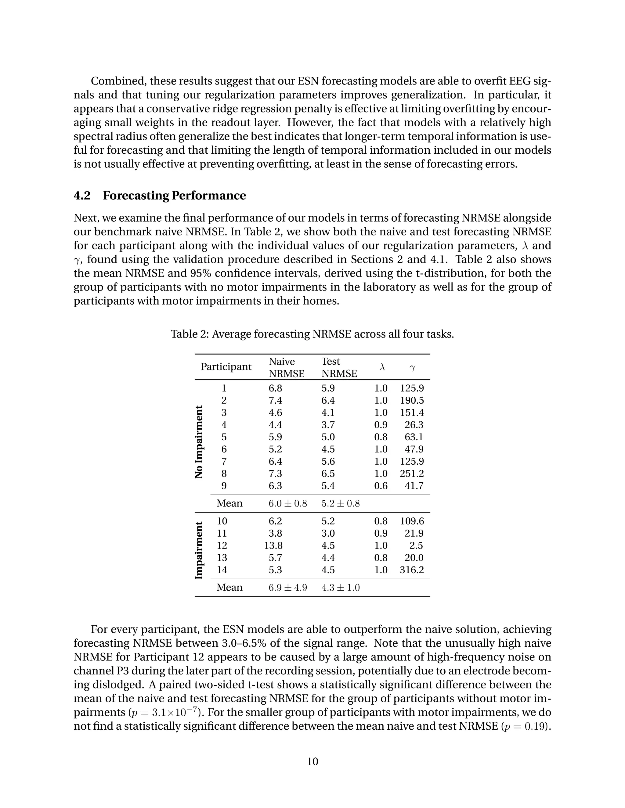
In order to present a more intuitive measure of forecasting error, we present our final results
as a percent of signal range using the normalized root-mean-squared error (NRMSE),
NRMSE =
100
signal max − signal min
ξ
N (T − 1)
. (8)
4.1 Forecasting Regularization
Now that we have established methods for modeling EEG signals and quantifying the resulting
errors, we continue by examining how our regularization parameters affect forecasting perfor-
mance. In Figure 4, we show how the training and validation NRMSE for Participant 4 change as
we vary the spectral radius and ridge regression penalty. These figures are representative of the
regularization process for all 14 participants.
Not surprisingly, the lowest training NRMSE is encountered when our regularization param-
eters impose little or no limitation on our model complexity, i.e., with a spectral radius near one
and a ridge regression penalty near zero. The lowest validation NRMSE, on the other hand, is
typically achieved with a spectral radius near one and a moderate ridge regression penalty.
0.2 0.4 0.6 0.8 1.0
Spectral Radius (λ)
RidgeRegressionPenalty(γ)
3.8
4.0
4.2
4.4
4.6
ForecastingError(NRMSE)
15251005002500
Lowest Validation Error
(a) Training NRMSE.
0.2 0.4 0.6 0.8 1.0
Spectral Radius (λ)
RidgeRegressionPenalty(γ)
5.0
5.5
6.0
ForecastingError(NRMSE)
15251005002500
Lowest Validation Error
(b) Validation NRMSE.
Figure 4: Training and validation forecasting NRMSE for Participant 4 as the spectral radius and
ridge regression penalty are varied. The lowest errors are typically achieved with a high spectral
radius. A moderate ridge regression penalty yields the best generalization.
9

11. Combined, these results suggest that our ESN forecasting models are able to overfit EEG sig-
nals and that tuning our regularization parameters improves generalization. In particular, it
appears that a conservative ridge regression penalty is effective at limiting overfitting by encour-
aging small weights in the readout layer. However, the fact that models with a relatively high
spectral radius often generalize the best indicates that longer-term temporal information is use-
ful for forecasting and that limiting the length of temporal information included in our models
is not usually effective at preventing overfitting, at least in the sense of forecasting errors.
4.2 Forecasting Performance
Next, we examine the final performance of our models in terms of forecasting NRMSE alongside
our benchmark naive NRMSE. In Table 2, we show both the naive and test forecasting NRMSE
for each participant along with the individual values of our regularization parameters, λ and
γ, found using the validation procedure described in Sections 2 and 4.1. Table 2 also shows
the mean NRMSE and 95% confidence intervals, derived using the t-distribution, for both the
group of participants with no motor impairments in the laboratory as well as for the group of
participants with motor impairments in their homes.
Table 2: Average forecasting NRMSE across all four tasks.
Participant
Naive
NRMSE
Test
NRMSE
λ γ
NoImpairment
1 6.8 5.9 1.0 125.9
2 7.4 6.4 1.0 190.5
3 4.6 4.1 1.0 151.4
4 4.4 3.7 0.9 26.3
5 5.9 5.0 0.8 63.1
6 5.2 4.5 1.0 47.9
7 6.4 5.6 1.0 125.9
8 7.3 6.5 1.0 251.2
9 6.3 5.4 0.6 41.7
Mean 6.0 ± 0.8 5.2 ± 0.8
Impairment
10 6.2 5.2 0.8 109.6
11 3.8 3.0 0.9 21.9
12 13.8 4.5 1.0 2.5
13 5.7 4.4 0.8 20.0
14 5.3 4.5 1.0 316.2
Mean 6.9 ± 4.9 4.3 ± 1.0
For every participant, the ESN models are able to outperform the naive solution, achieving
forecasting NRMSE between 3.0–6.5% of the signal range. Note that the unusually high naive
NRMSE for Participant 12 appears to be caused by a large amount of high-frequency noise on
channel P3 during the later part of the recording session, potentially due to an electrode becom-
ing dislodged. A paired two-sided t-test shows a statistically significant difference between the
mean of the naive and test forecasting NRMSE for the group of participants without motor im-
pairments (p = 3.1×10−7). For the smaller group of participants with motor impairments, we do
not find a statistically significant difference between the mean naive and test NRMSE (p = 0.19).
10

12. We do, however, arrive at a significant difference among the users with motor impairments if we
exclude Participant 12 (p = 4.6×10−3). These results suggest that ESN are able to learn meaning-
ful patterns in EEG that allow them to forecast the signal better than a single-timestep shift.
4.3 Iterated Models
In order to gain further insight into the patterns learned by our forecasting models, we also in-
vestigate the effects of placing a feedback loop from the output of a trained ESN back to the
network’s inputs. This forms an autonomous, self-driven system known as an iterated model.
These models may help illustrate the temporal behavior and internal dynamics of our forecast-
ing models.
In order to construct an iterated model, we first train an ESN to forecast eight seconds of
EEG. After the eight-second mark is reached, the network begins to use its past predictions as
input, instead of the true EEG. Over the course of the experiment, the output of the ESN can be
described by the recurrence relation
y(t) =
esn(s(t − 1)), if t < 8 · 256
esn(y(t − 1)), otherwise,
(9)
where s(t) is the true EEG signal at time t and 256 is the sampling frequency.
In Figure 5, we show an instance of this experiment two-seconds before and after the transi-
tion to an iterated model as the spectral radius, λ, is varied. Although all eight EEG channels were
used by the model, only channel P4 is shown for the sake of clarity. We note that these results
are largely representative of other channels and can be reproduced, with a degree of variation,
across reservoir initializations. With a relatively small spectral radius, less than about 0.4, the
output of our iterated model quickly dampens to zero. With a mid-range spectral radius, around
0.7, the output of our iterated model oscillates indefinitely with a predominant frequency that is
typically between 8–14Hz. As the spectral radius approaches one, our iterated model begins to
produce a sophisticated signal that appears to be similar to the true EEG.
In order to support our claim that iterated models with a large spectral radius produce output
similar similar to true EEG, we also examine energy spectra generated using continuous wavelet
transforms. In Figure 6a we show the energy spectrum of the same true EEG signal that is shown
in Figure 5. In Figure 6b, we show the energy spectrum of the signal produced by our iterated
model with a unit spectral radius, which is also shown in Figure 5c. Again, the forecasting model
is shown before the eight-second mark and the output of the iterated model is shown afterward.
Although the two clearly differ, both signals appear to have similar transient changes in energy
content across the frequency spectrum.
Although our forecasting models ultimately use only single-step-ahead predictions, our ex-
periments with iterated models lead us to several important conclusions. First, a small spectral
radius leads to models that include only very short-term temporal information. As the spectral
radius increases, the model becomes increasingly influenced by the more predominant oscilla-
tory components of the EEG signal. As the spectral radius approaches one, the ESN begins to
model high-frequency information as well as non-periodic and non-stationary dynamics. Fi-
nally, we believe that these experiments demonstrate that ESN are able to learn sophisticated
long-term patterns found in EEG.
11

13. (a) Iterated model with λ = 0.4
(b) Iterated model with λ = 0.7
(c) Iterated model with λ = 1.0
Figure 5: A trace illustrating an ESN transitioning from forecasting to an iterated model at the
eight-second mark. 5a) With a small spectral radius, the signal quickly dampens to zero. 5b)
With moderate spectral radius, the signal oscillates indefinitely with a frequency of about 12Hz.
5c) With a large spectral radius, the signal exhibits sophisticated dynamics similar to the true
EEG.
12

14. 6 7 8 9 10
10203040
Time (s)
Frequency(Hz)
1e−02
1e−01
1e+00
1e+01
1e+02
Energy
(a) Energy spectrum of true EEG.
6 7 8 9 10
10203040
Time (s)
Frequency(Hz)
1e−02
1e−01
1e+00
1e+01
1e+02
Energy
(b) Energy spectrum of ESN output.
Figure 6: Energy spectra of an ESN transitioning from forecasting to an iterated model at the
eight-second mark. 6a) The energy spectrum of the true EEG. 6b) The energy spectrum of the
ESN output. The ESN is forecasting before eight seconds and an iterated model afterward.
5 Classification
Now that we have demonstrated the ability of ESN to forecast EEG signals, we proceed by lever-
aging these models to construct EEG classifiers for use in BCI. In order to achieve this, we take
a generative approach. First, a separate ESN is trained to forecast sample EEG recorded during
each mental task. For a BCI that utilizes K different mental tasks, K different ESN are trained.
We then have an ESN associated with each mental task that can be viewed as an expert at fore-
casting the corresponding EEG signals.
Once these models are trained, previously unseen EEG is labeled by applying each ESN and
selecting the class label associated with model that best fits the signal. We achieve this by first
measuring the sum-squared forecasting error, as described in (6), for each ESN. The final class
label C is then
C = argmin
k∈{1,2,...,K}
ξk (10)
where ξk is the sum-squared forecasting error produced by the ESN trained to forecast the men-
tal task indexed by k and where K is the total number of mental tasks used. Although a sec-
ondary classifier could potentially be used to assign class labels by using these forecasting errors
as features, we have found that this best-fit approach typically works well without introducing
additional parameters [16].
In order to describe our results in a way that can be compared with other studies and that
conveys the type of experience that a BCI user might have, we use two classification perfor-
mance metrics. First, we report classification accuracy (CA) as percent correct classification at
two-second intervals. Although CA characterizes how often the classifier is correct, it can be
misleading because it does not take into account how many classes were used and the rate at
13

15. which class labels are assigned. For these reasons, we also report information transfer rate (ITR)
in bits-per-minute (bpm). We use the formulation of ITR that was adapted for use in BCI by
Wolpaw, et al. [41], using the work in information theory done by Pierce [42]. This definition of
ITR can be written as
ITR = V log2 K + P log2 P + (1 − P) log2
1 − P
K − 1
(11)
where V = 30 is the classification rate in decisions per minute, K is the number of classes and P
is the fraction of correct decisions over the total decisions made.
5.1 Classifier Regularization
Now that we have formalized our classifier, we continue by exploring how our regularization
parameters affect classification performance. Although we have established values for the spec-
tral radius and ridge regression penalty that achieve low forecasting errors, the same parameters
may not work well for classification. This is because noisy or undesirable components of an EEG
signal may be highly predictable in the sense of forecasting while not carrying information that
is useful for discriminating between mental tasks.
0.2 0.4 0.6 0.8 1.0
Spectral Radius (λ)
RidgeRegressionPenalty(γ)
30
40
50
60
70
80
90
100
PercentCorrect
15251005002500
Peak Validation CA
(a) Training accuracy.
0.2 0.4 0.6 0.8 1.0
Spectral Radius (γ)
RidgeRegressionPenalty(γ)
30
40
50
60
70
80
90
100
PercentCorrect
15251005002500
Peak Validation CA
(b) Validation accuracy.
Figure 7: Training and validation classification accuracy for Participant 1 as the spectral radius
and ridge regression penalty are varied. Validation accuracy peaks near the contour where the
training accuracy nears 100%, suggesting that overfitting is limited.
In Figure 7, we show the training and validation classification accuracies for Participant 1 as
the spectral radius and ridge regression penalty are varied. In this instance, we note that the
values for the spectral radius that produce the best validation classification accuracy are con-
siderably smaller than those that produce the lowest forecasting error. This suggests that some
of the more complex patterns that aid in forecasting are not helpful in discriminating between
mental tasks. We also notice that the best validation accuracy tends to occur along the contour
where training accuracy nears 100% correct. This suggests that our regularization parameters
14

16. are limiting overfitting by preventing our models from precisely fitting the data in the training
partition. It is important to note, however, that the topography of these experiments varies con-
siderably among the participants in our dataset.
5.2 Classifier Performance
Now that we have fully described our framework for using ESN to model and classify EEG, we re-
port our final classification results. First, we apply our classification algorithm to all four mental
tasks for each of our 14 participants. Class labels are assigned at non-overlapping two-second
intervals. Suitable values for our regularization parameters, λ and γ, are found on an individ-
ual basis using the procedures described in Sections 2 and 5.1. The final outcomes of these
experiments are displayed in Table 3, which includes training, validation and test classification
accuracies as well as test information transfer rates and the final values of our regularization pa-
rameters. The mean of our performance metrics along with 95% confidence intervals are also
reported for both groups of participants.
Table 3: Four-task performance results.
Participant
Training
CA (%)
Validation
CA (%)
Test
CA (%)
Test
ITR
(bpm)
λ γ
NoImpairment
1 97.5 71.7 62.5 13.5 0.2 5.0
2 100.0 50.0 42.5 3.1 0.8 1.0
3 92.1 53.3 55.0 8.8 0.2 95.5
4 100.0 68.3 65.0 15.3 0.8 8.7
5 98.8 46.7 45.0 4.1 0.2 0.7
6 100.0 71.7 62.5 13.5 0.5 0.7
7 88.8 55.0 40.0 2.3 1.0 3467.4
8 100.0 68.3 62.5 13.5 0.6 41.7
9 74.5 65.0 53.1 7.8 0.1 69.2
Mean 94.6 ± 6.6 61.1 ± 7.6 54.2 ± 7.4 9.1 ± 3.9
Impairment
10 92.9 51.7 27.5 0.1 0.9 912.0
11 100.0 65.0 55.0 8.8 1.0 69.2
12 93.3 41.7 15.0 0.0 0.1 0.0
13 100.0 60.0 56.2 9.5 0.9 10.5
14 65.8 45.0 37.5 1.6 0.2 3801.9
Mean 90.4 ± 17.6 52.7 ± 12.2 38.2 ± 22.0 4.0 ± 5.9
For the participants without motor impairments, we obtain test classification accuracies be-
tween 40–65% with a mean of 54 ± 7%. Since we have four mental tasks, a random classifier
would be expected to achieve a classification accuracy of only 25%. A t-test leads us to believe
that our mean classification accuracy is significantly better than chance (p = 1.8×10−5). A non-
parametric Wilcoxon Signed Ranks test agrees with this conclusion (p = 8.9×10−3). The infor-
mation transfer rates for this group range from 2–15bpm with a mean of 9 ± 4bpm, indicating
that every user in this group would be able to correctly issue at least some instructions to a BCI.
For the group of participants with motor impairments, classification accuracy ranges from
15–56% with a mean of 38 ± 22%. Among these participants, both a t-test (p = 0.17) and a
15

17. Wilcoxon test (p = 0.19) fail to conclude that our mean classification accuracy is better than
chance; however, these tests have less statistical power for this smaller group of participants.
The information transfer rates for this group range from 0–10bpm with a mean of 4 ± 6bpm.
Upon close inspection, it appears that these information transfer rates may have a bimodal dis-
tribution across participants; although Participants 10, 12 and 14 are able to attain little or no
information transfer, Participants 11 and 13 perform better than many of the participants with-
out motor impairments.
A comparison of the performance between the two groups leads to borderline results. A
two-sample, two-tailed t-test does not allow us to conclude a statistically significant difference
in mean classification accuracy between the participants with impairments and those without
impairments (p = 0.12). Similarly, a Mann-Whitney test, which may be more appropriate if
the results have a bimodal distribution, also does not allow us to conclude with a high degree
of certainty that there is a difference in mean classification accuracy between the groups (p =
0.094). However, the borderline p-values obtained from these tests and our observations about
the performance of individual participants appears to be consistent with the notion that fewer
people with impairments in home environments would be able to achieve an acceptable level of
performance.
Table 4: Four-task test confusion matrix for Participant 1.
Predicted (%)
Count Fist Rotate Song
Actual(%)
Count 100 0 0 0
Fist 50 30 10 10
Rotate 0 10 60 30
Song 20 20 0 60
Next, we seek to gain further insight into the types of misclassifications made by our algo-
rithm by examining confusion matrices. In Table 4, we display the confusion matrix of test clas-
sification accuracies for Participant 1. In this instance, we note that the error rates and types are
different for each mental task. For example, EEG segments that were recorded during the count
task are never mislabeled as another task, i.e., there are zero false-negatives. However, EEG seg-
ments recorded during the fist and song tasks are incorrectly labeled as the count task, i.e., false
positives, for 50% and 20% of segments, respectively.
Although individual confusion matrices can reveal the types of errors that occur for each
participant, we are also interested in discovering which, if any, mental tasks perform well in gen-
eral. One approach to answering this question is to examine the average confusion matrix for a
number of participants that achieve high classification accuracy. In Table 5, we show the mean
classification accuracies and 95% confidence intervals obtained by averaging the test confusion
matrices for all participants that achieve a test classification accuracy of 50% or greater, i.e., Par-
ticipants 1, 3, 4, 6, 8, 9, 11 and 13. Although the count task appears to have a relatively low false
positive rate, none of the other mental tasks clearly stands out as being advantageous. Further-
more, the mean classification accuracy is roughly the same for each of the four mental tasks and
the variability across each cell of the confusion matrices is relatively high. These observations
suggest that the best-performing mental tasks vary considerably among participants.
16

18. Table 5: Four-task test confusion matrix averaged across participants that achieve at least 50%
test classification accuracy.
Predicted (%)
Count Fist Rotate Song
Actual(%)
Count 65 ± 27 11 ± 8 11 ± 12 14 ± 15
Fist 15 ± 22 55 ± 20 21 ± 17 9 ± 5
Rotate 3 ± 4 15 ± 13 52 ± 12 30 ± 12
Song 8 ± 7 12 ± 11 22 ± 17 58 ± 20
Assuming that the best-performing mental tasks are user-specific, or perhaps even session-
specific, it seems appropriate for a BCI to select, during the calibration phase, which mental
tasks should be used. Next, we explore this possibility by performing two-task classification us-
ing only the two tasks that achieved the highest classification accuracy in the averaged confusion
matrix found during the validation procedure for each participant. Once the appropriate tasks
are selected, new regularization parameters are found and the classifier is re-trained. Although
using only the diagonal of the confusion matrix may not yield the best possible combination
of mental tasks, this approach is more practical for use in real-time systems than an exhaustive
search. Since only validation performance is used, this procedure avoids biasing our test results
and could conceivably be used during BCI training.
Table 6: Two-task performance results.
Participant
Training
CA (%)
Validation
CA (%)
Test
CA (%)
Test
ITR
(bpm)
λ γ Task 1 Task 2
NoImpairment
1 100.0 90.0 75.0 5.7 1.0 144.5 Count Song
2 100.0 90.0 80.0 8.3 0.4 3.6 Song Count
3 100.0 86.7 90.0 15.9 0.1 2.1 Song Fist
4 100.0 93.3 95.0 21.4 0.2 0.7 Rotate Fist
5 100.0 80.0 65.0 2.0 1.0 0.0 Count Rotate
6 100.0 96.7 95.0 21.4 1.0 0.5 Count Song
7 100.0 96.7 70.0 3.6 0.9 63.1 Fist Song
8 100.0 96.7 90.0 15.9 1.0 52.5 Fist Rotate
9 100.0 95.0 75.0 5.7 0.1 0.0 Count Fist
Mean 100.0 ± 0.0 91.7 ± 4.3 81.7 ± 8.6 11.1 ± 5.9
Impairment
10 100.0 80.0 40.0 0.0 1.0 0.5 Count Fist
11 100.0 90.0 70.0 3.6 0.9 14.5 Rotate Fist
12 90.0 80.0 50.0 0.0 0.1 0.0 Rotate Fist
13 100.0 95.0 87.5 13.7 1.0 11.0 Song Rotate
14 94.2 90.0 60.0 0.9 0.2 218.8 Song Count
Mean 96.8 ± 5.7 87.0 ± 8.3 61.5 ± 22.8 3.6 ± 7.2
In Table 6, we present the outcomes of these two-task experiments along with the tasks that
were selected for each participant. For the group of participants without motor impairments,
17

19. we achieve test classification accuracies between 65–95% with a mean of 82 ± 9%. Since we now
have two classes, a random classifier would be expected to achieve 50% classification accuracy.
A t-test confirms that our mean classification accuracy is significantly better than chance (p =
2.8×10−5) as does a Wilcoxon test (p = 9.0×10−3). The information transfer rates for this group
range from 2–21bpm with a mean of 11 ± 6bpm. This suggests that all users in this group would
be able to correctly issue at least some instructions to a BCI using only the two selected mental
tasks.
For the group of participants with motor impairments, our two-task experiments result in
classification accuracies ranging from 40–88% with a mean of 62±23%. For this smaller group of
participants, we are again unable to demonstrate that the mean classification accuracy is better
than chance using a t-test (p = 0.23) or Wilcoxon test (p = 0.27). The information transfer rates
for this group range from 0–14bpm with a mean of 4±7bpm. We also notice that the distribution
of the information transfer rates has a bimodal appearance with the same three participants
performing well in both the two-task and four-task scenarios.
For our two-task scenario, a comparison of the performance between the participants with
and without motor impairments again yields borderline results. Although a two-sample t-test
does not allow us to conclude with certainty that there is a difference in mean classification accu-
racy (p = 0.069), the non-parametric Mann-Whitney test does allow us to conclude a statistically
significant difference (p = 0.038). The results of these tests appear to suggest that fewer partic-
ipants with motor impairments would be able to achieve acceptable levels of performance in
our two-task scenario; although a larger group of participants is likely required in order to draw
firm conclusions. It is important to note, however, that one participant with motor impairments
performed quite well, achieving about 88% classification accuracy with a 14bpm information
transfer rate.
When comparing the difference in performance between the two-task and four-task scenar-
ios, we first notice that there is a relatively large difference in classification accuracy between
the two scenarios. For the participants without motor impairments a t-test (p = 4.6×10−5) and a
Mann-Whitney test (4.6×10−4) confirm that there is a statistically significant difference in mean
classification accuracy between the two scenarios. For the group of participants with motor
impairments, however, a t-test (p = 0.08) and Mann-Whitney test (p = 0.095) do not allow us
to conclude a statistically significant difference in mean classification accuracy; although the
results are somewhat borderline. An examination of the information transfer rates, however, re-
veals that there is very little difference in the amount of information that a BCI user would be
able to communicate in either scenario. In other words, the two-task scenario might yield a BCI
that makes fewer errors but the amount of work that a BCI user could accomplish is roughly the
same.
6 Conclusions
In the present work, we have described a method for constructing forecasting models of EEG us-
ing ESN. These models may be advantageous over other approaches because of their ability to
capture non-linear spatiotemporal patterns, their ability to be regularized and due to their com-
putational efficiency. The recurrent architecture of ESN also makes them natural fit for modeling
the transient oscillatory dynamics that are characteristic of EEG.
Using the configuration and parameter selection methods that we have outlined, we were
able to produce ESN that forecast EEG well, achieving error rates as low as 3% of the signal
range. Through iterated models, we were also able to show that ESN are capable of capturing
18

20. sophisticated patterns in EEG and that long-term, high-frequency and non-stationary patterns
are more prevalent in models that have a large spectral radius. We believe that these models
show considerable potential for capturing patterns in EEG and that they may have a number of
potential applications in BCI as well as broader EEG analysis.
We then proposed a straightforward generative classification algorithm that uses these fore-
casting models to label EEG in the context of mental-task BCI. This approach uses a separate
ESN for each mental task and assigns class labels according to the network that produces the
lowest forecasting error. We tested this classifier in an offline fashion on EEG recorded using a
portable eight-channel system from both participants without motor impairments in our lab-
oratory as well as participants with severe motor impairments in their home environments. To
our knowledge, we are the first to conduct experiments with mental-task BCI using EEG recorded
from participants with motor impairments in their home environments.
When using all four mental tasks, we achieved information transfer rates between 2–15bpm
for participants without motor impairments and 0–10bpm for participants with motor impair-
ments. We also observed that the mean classification accuracy for participants without motor
impairments was significantly higher than random and that the mean classification accuracy
for participants with motor impairments was borderline higher than random. Additionally, it
appears that the distribution of classification performance is somewhat bimodal, with some
participants performing quite well and others performing near random. These observations
lead us to two general conclusions. First, achieving consistently good results is more difficult
under realistic conditions. Second, it appears that some users with impairments may be able to
use such a BCI while others are may be unable to achieve an acceptable level of control.
We suspect that a combination of several factors is likely responsible for the differences in
performance among the participants with impairments. First, we observed considerably more
distraction in home environments than in our laboratory. For example, phones, pets and visi-
tors are frequent causes of distraction. Second, EEG sensor displacement can be a problem. For
instance, wheelchair headrests can make it difficult to maintain a good sensor-to-scalp connec-
tion following weight-shifts or other movements. Third, electrical interference is typically more
prominent in home environments. In one case, a source of strong 60Hz interference was iden-
tified as a hospital bed and the interference was not eliminated until the bed was unplugged
from the outlet. Finally, the various diseases and traumas that cause motor impairments could,
potentially, have an adverse effect on the EEG signals utilized by a BCI. Unfortunately, the influ-
ence of disease and trauma on EEG has not been well-characterized. Clearly, future BCI research
should consider these issues and focus on methods that are robust in real-world environments.
Although we obtained encouraging information transfer rates using four mental tasks, the
corresponding error rates were relatively high. This would likely lead to a level of frustration for
a user of an interactive BCI. In order to address this concern, we also explored the use of two
mental tasks, which were selected during the validation procedure. In this two-task scenario,
we achieved information transfer rates between 2–21bpm for the participants without motor
impairments and between 0–14bpm for the participants with motor impairments. Again, we
observed that the mean classification accuracy for participants without impairments was better
than random and the mean classification accuracy for participants with impairments was bor-
derline higher than random. We also again noted a bimodal distribution of performance across
participants with one participant with a motor impairment achieving an information transfer
rate of 14bpm. This suggests that some users may be able to use such a BCI under realistic con-
ditions.
Although the information transfer rates we observed were not significantly different between
the two and four-task scenarios, mean classification accuracy was significantly higher for the
19

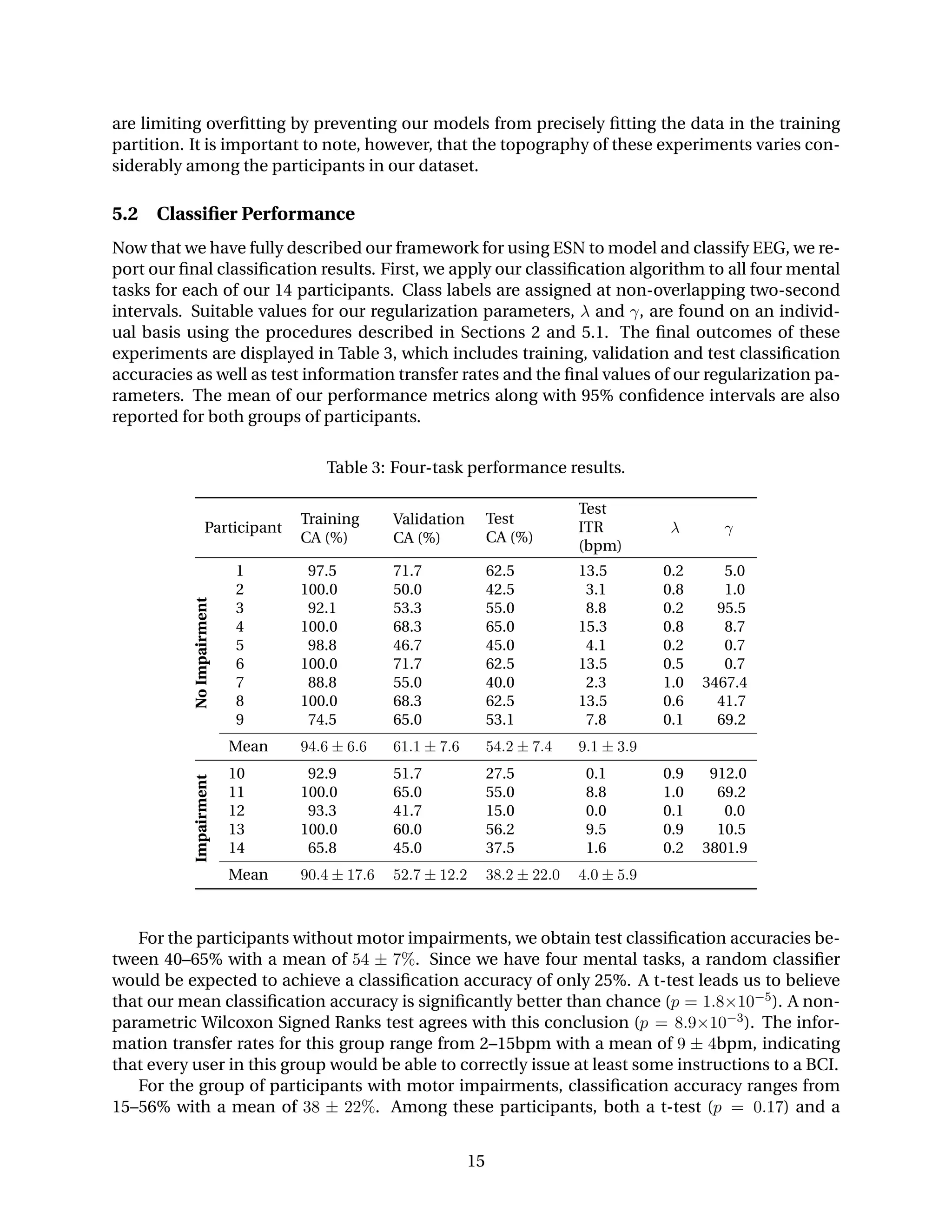
21. participants without impairments in the two-task scenario. This leads us to conclude that while
the two and four task scenarios would allow a BCI user to accomplish about the same amount
of work, the two-task scenario would lead to a lower error rate. Although a lower error rate may
be less frustrating for a BCI user, these gains come at the expense of fewer degrees of control.
In the present work, we have not directly compared our approach to other classification al-
gorithms. However, a review of current literature on mental-task BCI along with our estimate of
information transfer rate, computed using (11), suggests that offline performance ranges from
about 3–41bpm among state-of-the-art algorithms [7,9,12,19,20]. It is important to note, how-
ever, that the results at the high end of this range typically achieve moderate classification ac-
curacies with high information transfer rates because they assign class labels at intervals of less
than one second. These studies also only involve participants without motor impairments in
laboratory environments and typically use EEG acquisition systems with more channels and
higher sampling rates than the portable system used in the present work. In one study, however,
Millán, et al., performed online classification using a portable EEG system at a rate of about
2–80bpm after several consecutive days of training with feedback [20]. Although more compar-
ative work is clearly required, this review leads us to believe that our classification algorithm
performs on par with approaches that have been evaluated in offline settings and that training
with feedback may have the potential to improve performance considerably.
In our previous work, we explored a classifier that was similar to the approach described in
the present manuscript except that it used Elman Recurrent Neural Networks (ERNN) instead of
ESN [15,16]. In these works, we observed information transfer rates between 0–38bpm with de-
cisions made at one-second intervals for two participants without impairments and three partic-
ipants with severe motor impairments using a non-portable EEG system. Although we observed
a higher peak performance for ERNN, at least for some individuals, it is presently intractable to
train and perform parameter selection for ERNN in a real-time BCI. Therefore, a primary advan-
tage of ESN over ERNN is computational efficiency. However, a thorough comparison between
these two approaches is required in order to draw firm conclusions.
We believe that the next step in this line of research should be to explore modeling EEG at
multiple time-scales through multi-step predictions and iterated models. It is also important
to perform direct comparisons with other time-series models and classifiers in order to pre-
cisely quantify the advantages and disadvantages of these approaches. Additionally, we suspect
that more carefully designed filtering and artifact removal algorithms may lead to better per-
formance under realistic conditions. Finally, we feel that it is important to conduct interactive
experiments. Since the ability to control computerized devices is the final goal of assistive BCI
and because users may learn to improve performance in the presence of feedback, real-time
experiments should be a focal point of future BCI research.
References
[1] Luis Nicolas-Alonso and Jaime Gomez-Gil. Brain computer interfaces, a review. Sensors,
12(2):1211–1279, 2012.
[2] Jean-Dominique Bauby. The diving bell and the butterfly: A memoir of life in death. Vintage,
1998.
[3] Eric Sellers, Theresa Vaughan, and Jonathan Wolpaw. A brain-computer interface for long-
term independent home use. Amyotrophic lateral sclerosis, 11(5):449–455, 2010.
20

22. [4] Guido Dornhege. Toward brain-computer interfacing. The MIT Press, 2007.
[5] Jonathan Wolpaw and Elizabeth Winter Wolpaw. Brain-computer interfaces: principles and
practice. Oxfort University Press, 2012.
[6] Paul Nunez and Ramesh Srinivasan. Electric fields of the brain: the neurophysics of EEG.
Oxford University Press, USA, 2006.
[7] Zachary Keirn and Jorge Aunon. A new mode of communication between man and his
surroundings. IEEE Transactions on Biomedical Engineering, 37(12):1209–1214, 1990.
[8] Charles Anderson, Erik Stolz, and Sanyogita Shamsunder. Discriminating mental tasks us-
ing EEG represented by AR models. In 17th Annual Conference of The IEEE Engineering in
Medicine and Biology Society, volume 2, pages 875–876. IEEE, 1995.
[9] Charles Anderson, Erik Stolz, and Sanyogita Shamsunder. Multivariate autoregressive mod-
els for classification of spontaneous electroencephalographic signals during mental tasks.
IEEE Transactions on Biomedical Engineering, 45(3):277–286, 1998.
[10] Charles Anderson, James Knight, Tim O’Connor, Michael Kirby, and Artem Sokolov. Geo-
metric subspace methods and time-delay embedding for EEG artifact removal and classifi-
cation. IEEE Transactions on Neural Systems and Rehabilitation Engineering, 14(2):142–146,
2006.
[11] Charles Anderson, James Knight, Michael Kirby, and Douglas Hundley. Classification
of time-embedded EEG using short-time principal component analysis. Toward Brain-
Computer Interfacing, pages 261–278, 2007.
[12] Charles Anderson and Jeshua Bratman. Translating thoughts into actions by finding pat-
terns in brainwaves. In Proceedings of the Fourteenth Yale Workshop on Adaptive and Learn-
ing Systems, pages 1–6, 2008.
[13] Charles Anderson, Elliott Forney, Douglas Hains, and Annamalai Natarajan. Reliable identi-
fication of mental tasks using time-embedded EEG and sequential evidence accumulation.
Journal of Neural Engineering, 8(2):025023, 2011.
[14] Damien Coyle, Girijesh Prasad, and Thomas McGinnity. A time-series prediction approach
for feature extraction in a brain-computer interface. IEEE Transactions on Neural Systems
and Rehabilitation Engineering, 13(4):461–467, 2005.
[15] Elliott Forney and Charles Anderson. Classification of EEG during imagined mental tasks by
forecasting with elman recurrent neural networks. International Joint Conference on Neural
Networks (IJCNN), pages 2749–2755, 2011.
[16] Elliott Forney. Electroencephalogram classification by forecasting with recurrent neural
networks. Master’s thesis, Department of Computer Science, Colorado State University,
Fort Collins, CO, 2011.
[17] Elliott Forney, Charles Anderson, William Gavin, and Patricia Davies. A stimulus-free brain-
computer interface using mental tasks and echo state networks. In Proceedings of the Fifth
International Brain-Computer Interface Meeting: Defining the Future. Graz University of
Technology Publishing House, 2013.
21

23. [18] Elisabeth Friedrich, Reinhold Scherer, and Christa Neuper. The effect of distinct mental
strategies on classification performance for brain–computer interfaces. International Jour-
nal of Psychophysiology, 84(1):86–94, 2012.
[19] Elisabeth Friedrich, Reinhold Scherer, and Christa Neuper. Long-term evaluation of a 4-
class imagery-based brain–computer interface. Clinical Neurophysiology, 2013.
[20] José Millán, Josep Mouriño, Marco Franzé, Febo Cincotti, Markus Varsta, Jukka Heikkonen,
and Fabio Babiloni. A local neural classifier for the recognition of EEG patterns associated
to mental tasks. IEEE Transactions on Neural Networks, 13(3):678–686, 2002.
[21] José Millán, Frédéric Renkens, Josep Mouriño, and Wulfram Gerstner. Brain-actuated in-
teraction. Artificial Intelligence, 159(1):241–259, 2004.
[22] José Millán, Pierre Ferrez, Ferran Galán, Eileen Lew, and Ricardo Chavarriaga. Non-invasive
brain-machine interaction. International Journal of Pattern Recognition and Artificial In-
telligence, 22(05):959–972, 2008.
[23] Ferran Galán, Marnix Nuttin, Eileen Lew, Pierre Ferrez, Gerolf Vanacker, Johan Philips, and
José Millán. A brain-actuated wheelchair: Asynchronous and non-invasive brain-computer
interfaces for continuous control of robots. Clinical Neurophysiology, 119(9):2159–2169,
2008.
[24] Li Zhiwei and Shen Minfen. Classification of mental task EEG signals using wavelet packet
entropy and SVM. In 8th International Conference on Electronic Measurement and Instru-
ments, pages 3–906. IEEE, 2007.
[25] Gert Pfurtscheller. Event-related synchronization (ers): an electrophysiological correlate
of cortical areas at rest. Electroencephalography and clinical neurophysiology, 83(1):62–69,
1992.
[26] Elisabeth Friedrich, Reinhold Scherer, and Christa Neuper. Do user-related factors of mo-
tor impaired and able-bodied participants correlate with classification accuracy? In Proc-
ceedings of the 5th International Brain-Computer Interface Conference, pages 156–159. Graz
University of Technology, 2011.
[27] Zachary Cashero. Comparison of EEG preprocessing methods to improve the performance
of the P300 speller. Master’s thesis, Department of Computer Science, Colorado State Uni-
versity, Fort Collins, CO, 2011.
[28] Damien Coyle, Girijesh Prasad, and Thomas McGinnity. Extracting features for a brain-
computer interface by self-organising fuzzy neural network-based time series prediction.
In 26th Annual International Conference of The IEEE Engineering in Medicine and Biology
Society, volume 2, pages 4371–4374. IEEE, 2004.
[29] Damien Coyle, Thomas McGinnity, and Girijesh Prasad. Creating a nonparametric brain-
computer interface with neural time-series prediction preprocessing. In 28th Annual Inter-
national Conference of The IEEE Engineering in Medicine and Biology Society, pages 2183–
2186. IEEE, 2006.
[30] Damien Coyle, Thomas McGinnity, and Girijesh Prasad. A multi-class brain-computer in-
terface with SOFNN-based prediction preprocessing. In The 2008 International Joint Con-
ference on Neural Networks (IJCNN), pages 3696–3703. IEEE, 2008.
22

24. [31] Vaibhav Gandhi, Vipul Arora, Laxmidhar Behera, Girijesh Prasad, Damien Coyle, and
Thomas McGinnity. EEG denoising with a recurrent quantum neural network for a brain-
computer interface. In The 2011 International Joint Conference on Neural Networks (IJCNN),
pages 1583–1590. IEEE, 2011.
[32] Vaibhav Gandhi, Girijesh Prasad, Damien Coyle, Laxmidhar Behera, and Thomas McGin-
nity. Quantum neural network-based EEG filtering for a brain-computer interface. IEEE
Transactions on Neural Networks and Learning Systems, 25(2):278–288, 2014.
[33] Herbert Jaeger. Tutorial on training recurrent neural networks, covering BPTT, RTRL, EKF
and the echo state network approach. GMD Report 159: German National Research Center
for Information Technology, 2002.
[34] Herbert Jaeger. Adaptive nonlinear system identification with echo state networks. In Ad-
vances in Neural Information Processing Systems (Proceedings of NIPS 15), volume 15, pages
593–600. MIT Press, 2003.
[35] Herbert Jaeger and Harald Haas. Harnessing nonlinearity: Predicting chaotic systems and
saving energy in wireless communication. Science, 304(5667):78–80, 2004.
[36] Elliott Forney, Charles Anderson, Patricia Davies, William Gavin, Brittany Taylor, and Marla
Roll. A comparison of EEG systems for use in P300 spellers by users with motor im-
pairments in real-world environments. In Proceedings of the Fifth International Brain-
Computer Interface Meeting: Defining the Future. Graz University of Technology Publishing
House, 2013.
[37] William Gavin and Patricia Davies. Obtaining reliable psychophysiological data with child
participants. Developmental Psychophysiology: Theory, Systems, and Methods. Cambridge
University Press, New York, NY, pages 424–447, 2008.
[38] College of Health and Human Sciences at Colorado State University. Brainwaves research
laboratory. http://brainwaves.colostate.edu, Oct 2015.
[39] Department of Compter Science at Colorado State University. CEBL: CSU EEG and Brain-
Computer Interface Laboratory. http://www.cs.colostate.edu/eeg/main/software/
cebl3, Oct 2015.
[40] Fraunhofer Institute for Intelligent Analysis and Information Systems. International Patent
No. WO/2002/031764, 2002.
[41] Jonathan Wolpaw, Herbert Ramoser, Dennis McFarland, and Gert Pfurtscheller. EEG-based
communication: improved accuracy by response verification. IEEE Transactions on Reha-
bilitation Engineering, 6(3):326–333, 1998.
[42] John Pierce. An introduction to information theory: symbols, signals & noise. Dover, 1980.
23