Download to read offline
![Forecasting Temperatures in Bangladesh: An Application of SARIMA Models
Doulah 109
employment. In addition, more than 70% of Bangladesh
population living in rural areas depends on agricultural
related activities for their daily livelihoods. Climatic studies
on temperature are therefore vital for the survival of the
agricultural sector as the key source of revenue to the
government of Bangladesh.
Temperature is one of the key elements of climate and it is
important to various sectors of the economy like
Agriculture. Temperature affects water sources, pests that
attack plants, animals and human diseases. Despite the
increasing climate changes, majority of Bangladeshi
citizens are still not well informed. Analyzing and
forecasting of temperature changes will thus help various
stakeholders and government to plan in advance in order
to counter climate related disasters. The objective of this
research is to build a time series model and use this model
to analyze and forecast the variation in maximum and
minimum temperature in Bangladesh in order to inform
stakeholders who depend directly or indirectly on it to plan
in advance.
METHODOLOGY
Average Maximum and Minimum Monthly temperature
data covering Bangladesh has been collected from the
Bangladesh Meteorological Department (BMD). This data
was recorded in monthly basis covering an 18 year period
from January 2000 to December 2017 (www.data.gov.bd).
The temperatures are measured in degrees Celsius. The
temperature data is a continuous univariate time series as
it contains a single variable (temperature) which is
measured at every instant of time. However, this data was
merged into monthly intervals transforming it to a discrete
univariate time series.
The Box-Jenkins Method
This study follows the Box-Jenkins methodology for
modeling. The following conceptual framework proposed
by Box et al. (1976) is considered in this study.
Figure 1. Box- Jenkins ARIMA Model
Seasonal ARIMA (SARIMA) Model
Gurudeo and Mahbub (2010) alludes that most natural
factors like temperature have strong seasonal
Components. It is therefore necessary to use
autoregressive and moving average polynomials that
identify with the seasonal lags. One such model is the
SARIMA model. SARIMA model is an extension of ARIMA
model and it is applied when the series contains both
seasonal and non-seasonal behavior. SARIMA model is
sometimes called the multiplicative seasonal
autoregressive integrated moving average and is denoted
by SARIMA (p,d,q)(P,D,Q)S. The Seasonal AR can be
written as:
tt
s
p yB )(
The Seasonal MA can be written as
t
s
Qt By )(
The seasonal differencing is expressed as
sttt
s
yyyB )1(
Combining the above equations, we get SARIMA
t
s
Qqt
Dsds
pp BByBBBB )()()1()1)(()( 0
Where the constant equals
)]1)(1[( 110 pp
Where p represents non-seasonal AR order, d represents
non seasonal differencing, q represents non seasonal MA
order, P represents seasonal AR order, D represents
seasonal differencing, Q represents seasonal MA order, S
represents seasonal order (for monthly data S = 12 ) ty
represents time series data at period t, B is the backward
shift operator (
k
t t kB y y ) and t is the random shock
(white noise error).
Stationarity Analysis
One of the important types of data used in empirical
analysis is time series data. The empirical work based on
time series data assumes that the underlying time series
is stationary. The time series analysis based on the
stationary time series data. In this section we briefly
discuss on stationary and non-stationary time series. A
stochastic process is said to be stationary if its mean and
variance are constant over time. Otherwise it will be non-
stationary. Why are stationary time series so important?
Because if a time series is non-stationary, we can study its
behavior only for the time period under consideration.
Each set of time series data will therefore be for a
particular episode. As a consequence, it is not possible to
generalize it to other time periods. Therefore, for the
purpose of forecasting, such (non-stationary) time series
may be of little practical value. How do we know that a
particular time series is stationary? There are several tests
of stationary. Here we used graphical and analytical
recognized test. Graphical test: if we depend on common
sense, it would seem that the time series depicted in figure](https://image.slidesharecdn.com/pdf-180918151412/75/Forecasting-Temperatures-in-Bangladesh-An-Application-of-SARIMA-Models-2-2048.jpg)
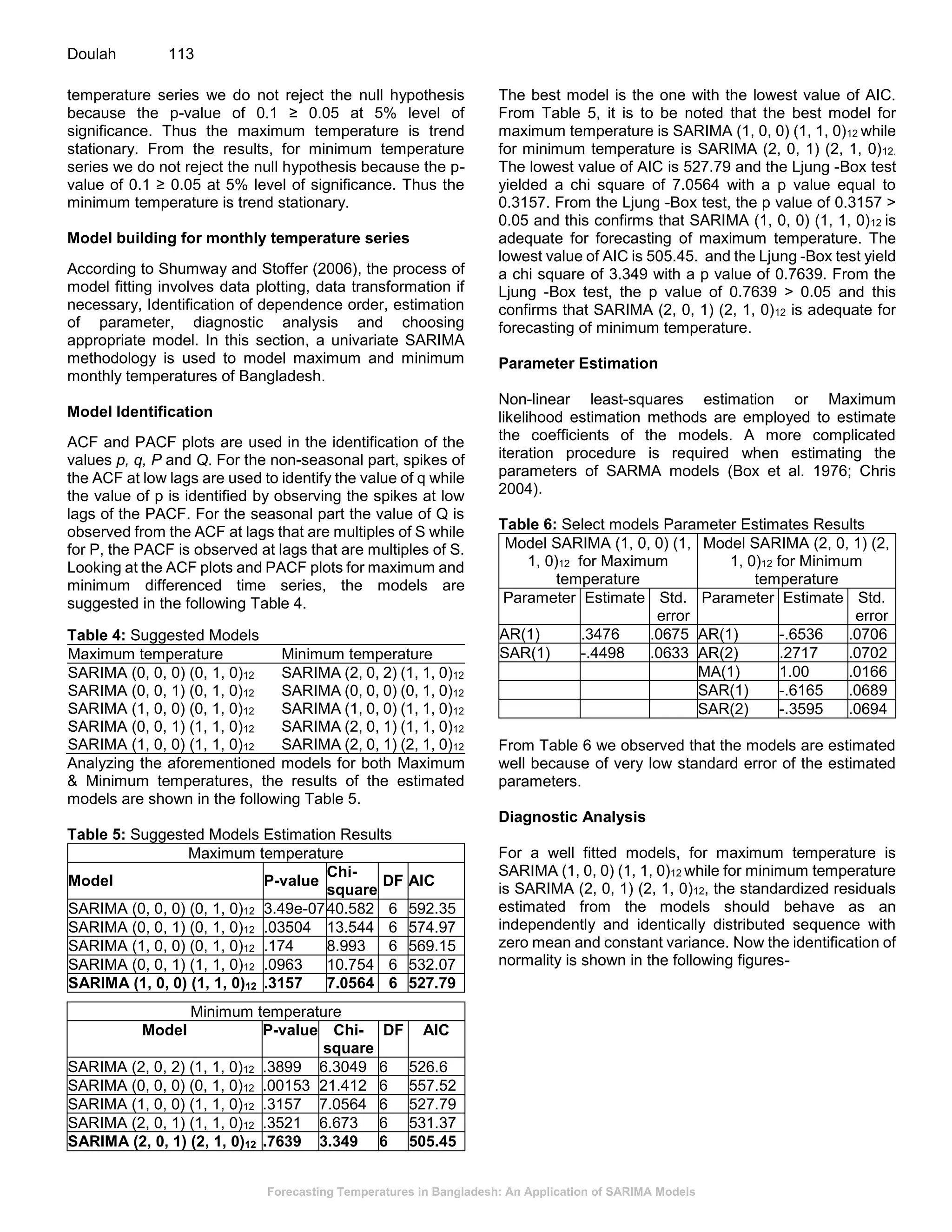
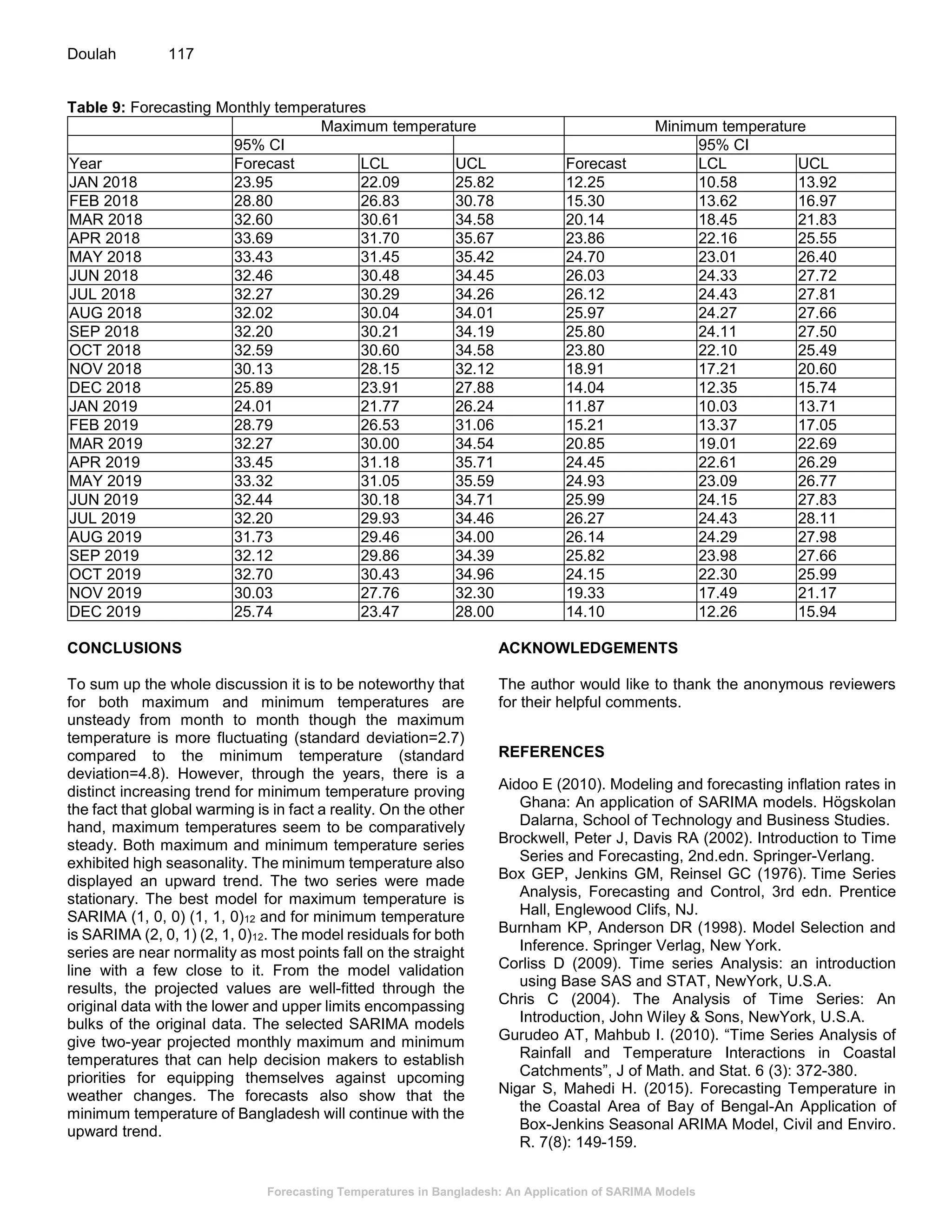

This document presents a study on forecasting temperatures in Bangladesh using SARIMA models, highlighting the significant fluctuations in minimum temperatures compared to maximum temperatures. The best models identified for maximum and minimum temperatures are SARIMA(1, 0, 0)(1, 1, 0)12 and SARIMA(2, 0, 1)(2, 1, 0)12, respectively, with validation showing accurate fitting to original data. The forecasts predict an upward trend in minimum temperatures, indicating the necessity for climate-related planning in sectors such as agriculture, which is vital for the Bangladeshi economy.


![11.[1 11]a seasonal arima model for nigerian gross domestic product](https://cdn.slidesharecdn.com/ss_thumbnails/11-1-11aseasonalarimamodelfornigeriangrossdomesticproduct-120512235353-phpapp02-thumbnail.jpg?width=640&height=640&fit=bounds)
![11.[1 11]a seasonal arima model for nigerian gross domestic product](https://cdn.slidesharecdn.com/ss_thumbnails/11-1-11aseasonalarimamodelfornigeriangrossdomesticproduct-120512235426-phpapp02-thumbnail.jpg?width=640&height=640&fit=bounds)


