This chapter covers the fundamentals of forecasting in operations management, including its importance, methods, and the factors that influence forecast accuracy. Key learning objectives include understanding forecast features, techniques (both qualitative and quantitative), and how to calculate and monitor forecast errors. It emphasizes the necessity for accurate forecasts in various business functions such as finance, human resources, and marketing.

1. © McGraw Hill 1
Chapter 3
Forecasting
Operations Management
FOURTEENTH EDITION
William J. Stevenson
© 2021 McGraw Hill. All rights reserved. Authorized only for instructor use in the

2. © McGraw Hill 2
Chapter 3: Learning Objectives
You should be able to:
LO 3.1 List features common to all forecasts
LO 3.2 Explain why forecasts are generally wrong
LO 3.3 List the elements of a good forecast
LO 3.4 Outline the steps in the forecasting process
LO 3.5 Summarize forecast errors and use summaries to make decisions
LO 3.6 Describe four qualitative forecasting techniques
LO 3.7 Use a naïve method to make a forecast
LO 3.8 Prepare a moving average forecast
LO 3.9 Prepare a weighted-average forecast
LO 3.10 Prepare an exponential smoothing forecast
LO 3.11 Prepare a linear trend forecast
LO 3.12 Prepare a trend-adjusted exponential smoothing forecast
LO 3.13 Compute and use seasonal relatives
LO 3.14 Compute and use regression and correlation coefficients
LO 3.15 Construct control charts and use them to monitor forecast errors
LO 3.16 Describe the key factors and trade-offs to consider when choosing a
forecasting technique

3. © McGraw Hill 3
Forecast
LO 3.1
Forecast – a statement about the future value of a
variable of interest
We make forecasts about such things as weather, demand,
and resource availability
Forecasts are important to making informed decisions

4. © McGraw Hill 4
Two Important Aspects of Forecasts
LO 3.1
Expected level of demand
The level of demand may be a function of some structural
variation such as trend or seasonal variation
Accuracy
Related to the potential size of forecast error

5. © McGraw Hill 5
Forecasts in Business Organizations
LO 3.1
Accounting. New product/process cost estimates, profit projections,
cash management.
Finance. Equipment/equipment replacement needs, timing
and amount of funding/borrowing needs.
Human resources. Hiring activities, including recruitment,
interviewing, and training; layoff planning, including
outplacement counseling.
Marketing. Pricing and promotion, e-business strategies, global
competition strategies.
MIS. New/revised information systems, internet services.
Operations. Schedules, capacity planning, work assignments and
workloads, inventory planning, make-or-buy decisions, outsourcing,
project management.
Product/service design. Revision of current features, design of new
products or services.

6. © McGraw Hill 6
Forecast Uses
LO 3.1
Plan the system
Generally involves long-range plans related to:
• Types of products and services to offer
• Facility and equipment levels
• Facility location
Plan the use of the system
Generally involves short- and medium-range plans related to:
• Inventory management
• Workforce levels
• Purchasing
• Production
• Budgeting
• Scheduling

7. © McGraw Hill 7
Features Common to All Forecasts
LO 3.1
1. Techniques assume some underlying causal system that
existed in the past will persist into the future
2. Forecasts are not perfect
3. Forecasts for groups of items are more accurate than
those for individual items
4. Forecast accuracy decreases as the forecasting horizon
increases

8. © McGraw Hill 8
Forecasts Are Not Perfect
LO 3.2
Forecasts are not perfect:
• Because random variation is always present, there will
always be some residual error, even if all other factors
have been accounted for.

9. © McGraw Hill 9
Elements of a Good Forecast
LO 3.3
The forecast
• Should be timely
• Should be accurate
• Should be reliable
• Should be expressed in meaningful units
• Should be in writing
• Technique should be simple to understand and use
• Should be cost-effective

10. © McGraw Hill 10
Steps in the Forecasting Process
LO 3.4
1. Determine the purpose of the forecast
2. Establish a time horizon
3. Obtain, clean, and analyze appropriate data
4. Select a forecasting technique
5. Make the forecast
6. Monitor the forecast errors

11. © McGraw Hill 11
Forecasting Approaches
LO 3.6
Qualitative forecasting
Qualitative techniques permit the inclusion of soft information
such as:
• Human factors
• Personal opinions
• Hunches
These factors are difficult, or impossible, to quantify
Quantitative forecasting
These techniques rely on hard data
Quantitative techniques involve either the projection of
historical data or the development of associative methods
that attempt to use causal variables to make a forecast

12. © McGraw Hill 12
Qualitative Forecasts
LO 3.6
Forecasts that use subjective inputs such as opinions from consumer surveys,
sales staff, managers, executives, and experts
Executive opinions
• A small group of upper-level managers may meet and collectively develop a forecast
Salesforce opinions
• Members of the sales or customer service staff can be good sources of information
due to their direct contact with customers and may be aware of plans customers may
be considering for the future
Consumer surveys
• Since consumers ultimately determine demand, it makes sense to solicit input from
them
• Consumer surveys typically represent a sample of consumer opinions
Other approaches
• Managers may solicit opinions from other managers or staff people or outside
experts to help with developing a forecast
• The Delphi method is an iterative process intended to achieve a consensus

13. © McGraw Hill 13
Time-Series Forecasts
LO 3.6
Forecasts that project patterns identified in recent time-series
observations
Time-series – a time-ordered sequence of observations
taken at regular time intervals
Assume that future values of the time-series can be
estimated from past values of the time-series

14. © McGraw Hill 14
Time-Series Behaviors
LO 3.6
Trend
Seasonality
Cycles
Irregular variations
Random variation

15. © McGraw Hill 15
Trends and Seasonality
LO 3.6
Trend
A long-term upward or downward movement in data
• Population shifts
• Changing income
Seasonality
Short-term, fairly regular variations related to the calendar or
time of day
Restaurants, service call centers, and theaters all experience
seasonal demand

16. © McGraw Hill 16
Cycles and Variations
LO 3.6
Cycle
Wavelike variations lasting more than one year
• These are often related to a variety of economic, political, or even
agricultural conditions
Irregular variation
Due to unusual circumstances that do not reflect typical
behavior
• Labor strike
• Weather event
Random Variation
Residual variation that remains after all other behaviors have
been accounted for

17. © McGraw Hill 17
Time-Series Forecasting - Naïve Forecast
LO 3.7
Naïve forecast
Uses a single previous value of a time series as the basis for
a forecast
• The forecast for a time period is equal to the previous time period’s
value
Can be used with
• A stable time series
• Seasonal variations
• Trend

18. © McGraw Hill 18
Time-Series Forecasting - Averaging
LO 3.7
These techniques work best when a series tends to vary
about an average
Averaging techniques smooth variations in the data
They can handle step changes or gradual changes in the
level of a series
Techniques
1. Moving average
2. Weighted moving average
3. Exponential smoothing

19. © McGraw Hill 19
Moving Average 1
LO 3.8
Technique that averages a number of the most recent actual
values in generating a forecast
where
1 2 1
MA
n
t i
i t n t t
t n
A
A A A
F
n n
−
= − − −
+ + +
= = =

Forecast for time period
MA period moving average
Actual value in period
Number of periods in the moving average
t
n
t i
F t
n
A t i
n
−
=
=
= −
=

20. © McGraw Hill 20
Moving Average 2
LO 3.7
As new data become available, the forecast is updated by
adding the newest value and dropping the oldest and then
recomputing the average
The number of data points included in the average
determines the model’s sensitivity
Fewer data points used—more responsive
More data points used—less responsive

21. © McGraw Hill 21
Weighted Moving Average
LO 3.9
The most recent values in a time series are given more
weight in computing a forecast
The choice of weights, w, is somewhat arbitrary and involves
some trial and error
where
1 1
( ) ( ) ( )
t t t t t t n t n
F w A w A w A
− − − −
= + + +
1
1
weight for period , weight for period 1, etc.
the actual value for period , the actual value for period 1, etc.
t t
t t
w t w t
A t A t
−
−
= = −
= = −

22. © McGraw Hill 22
Exponential Smoothing
LO 3.10
A weighted averaging method that is based on the previous
forecast plus a percentage of the forecast error
where
1 1 1
( )
t t t t
F F A F

− − −
= + −
1
1
Forecast for period
Forecast for the previous period
Smoothing constant
Actual demand or sales for the previous period
t
t
t
F t
F
A

−
−
=
=
=
=

23. © McGraw Hill 23
Linear Trend
LO 3.11
A simple data plot can reveal the existence and nature of a
trend
Linear trend equation
where
t
F a bt
= +
Forecast for period
Value of at 0
Slope of the line
Specified number of time periods from 0
t
t
F t
a F t
b
t t
=
= =
=
= =

24. © McGraw Hill 24
Estimating Slope and Intercept
LO 3.11
Slope and intercept can be estimated from historical data
where
( )
2
2
or
n ty t y
b
n t t
y b t
a y bt
n
−
=
−
−
= −
  
 
 
Number of periods
Value of the time series
n
y
=
=

25. © McGraw Hill 25
Trend-Adjusted Exponential Smoothing1
LO 3.12
The trend adjusted forecast consists of two components
Smoothed error
Trend factor
where
1
TAFt t t
S T
+ = +
Previous forecast plus smoothed error
Current trend estimate
t
t
S
T
=
=

26. © McGraw Hill 26
Trend-Adjusted Exponential Smoothing2
LO 3.12
Alpha and beta are smoothing constants
Trend-adjusted exponential smoothing has the ability to
respond to changes in trend
1
1 1 1
TAF
TAF ( TAF )
(TAF TAF )
t t t
t t t t
t t t t t
S T
S A
T T T


+
− − −
= +
= + −
= + − −

27. © McGraw Hill 27
Techniques for Seasonality
LO 3.12
Seasonality – regularly repeating movements in series
values that can be tied to recurring events
Expressed in terms of the amount that actual values deviate
from the average value of a series
Models of seasonality
• Additive
• Seasonality is expressed as a quantity that gets added to or subtracted
from the time-series average in order to incorporate seasonality
• Multiplicative
• Seasonality is expressed as a percentage of the average (or trend)
amount which is then used to multiply the value of a series in order to
incorporate seasonality

28. © McGraw Hill 28
Seasonal Relatives
LO 3.13
Seasonal relatives
The seasonal percentage used in the multiplicative
seasonally adjusted forecasting model
Using seasonal relatives
To deseasonalize data
• Done in order to get a clearer picture of the nonseasonal (for
example, trend) components of the data series
• Divide each data point by its seasonal relative
To incorporate seasonality in a forecast
1. Obtain trend estimates for desired periods using a trend equation
2. Add seasonality by multiplying these trend estimates by the
corresponding seasonal relative

29. © McGraw Hill 29
Associative Forecasting Techniques
LO 3.14
Associative techniques are based on the development of an
equation that summarizes the effects of predictor variables
Predictor variables – variables that can be used to predict
values of the variable of interest
• Home values may be related to such factors as home and property
size, location, number of bedrooms, and number of bathrooms

30. © McGraw Hill 30
Simple Linear Regression
LO 3.14
Regression – a technique for fitting a line to a set of data
points
Simple linear regression – the simplest form of regression
that involves a linear relationship between two variables
• The object of simple linear regression is to obtain an equation of a
straight line that minimizes the sum of squared vertical deviations
from the line (that is, the least squares criterion)

31. © McGraw Hill 31
Least Squares Line
LO 3.14
where
and
where
e
y a bx
= +
= Predicted (dependent) variable
= Predictor (independent) variable
= Slope of the line
= Value of when 0 (that is, the height of the line at the intercept)
c
c
y
x
b
a y x y
=
( ) ( )( )
( ) ( )
2
2
or
n xy x y
b
n x x
y b x
a y bx
n
−
=
−
−
= −
  
 
 
Number of paired observations
n =

32. © McGraw Hill 32
Correlation Coefficient
LO 3.14
Correlation, r
A measure of the strength and direction of relationship
between two variables
Ranges between −1.00 and +1.00
r2, square of the correlation coefficient
A measure of the percentage of variability in the values of y
that is “explained” by the independent variable
Ranges between 0 and 1.00
( ) ( )( )
( ) ( ) ( ) ( )
2 2
2 2
n xy x y
r
n x x n y y
−
=
− −
  
   

33. © McGraw Hill 33
Simple Linear Regression Assumptions
LO 3.14
1. Variations around the line are random
2. Deviations around the average value (the line) should be
normally distributed
3. Predictions are made only within the range of observed
values

34. © McGraw Hill 34
Issues to Consider:
LO 3.14
Always plot the line to verify that a linear relationship is
appropriate
The data may be time-dependent
If they are
• use analysis of time series
• use time as an independent variable in a multiple regression
analysis
A small correlation may indicate that other variables are
important

35. © McGraw Hill 35
Forecast Accuracy and Control
LO 3.5
Allowances should be made for forecast errors
It is important to provide an indication of the extent to which
the forecast might deviate from the value of the variable that
actually occurs
Forecast errors should be monitored
Error = Actual − Forecast
If errors fall beyond acceptable bounds, corrective action
may be necessary

36. © McGraw Hill 36
Forecast Accuracy Metrics
LO 3.5
MAD weights all errors evenly
MSE weights errors according
to their squared values
MAPE weights errors
according to relative error
t t
Actual Forecast
MAD
n
−
=

( )
2
t t
Actual Forecast
MSE
1
n
−
=
−

t t
t
Actual Forecast
100
Actual
MAPE
n
−

=


37. © McGraw Hill 37
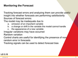
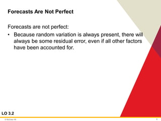
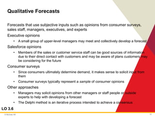
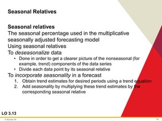
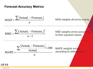
Forecast Error Calculation
LO 3.5
Period
Actual
(A)
Forecast
(F)
(A − F)
Error |Error| Error2 [|Error|/Actual] × 100
1 107 110 −3 3 9 2.80%
2 125 121 4 4 16 3.20%
3 115 112 3 3 9 2.61%
4 118 120 −2 2 4 1.69%
5 108 109 1 1 1 0.93%
Sum 13 39 11.23%
n = 5 n − 1 = 4 n = 5
MAD MSE MAPE
= 2.6 = 9.75 = 2.25%

38. © McGraw Hill 38
Monitoring the Forecast
LO 3.15
Tracking forecast errors and analyzing them can provide useful
insight into whether forecasts are performing satisfactorily
Sources of forecast errors:
The model may be inadequate due to
a. omission of an important variable
b. a change or shift in the variable the model cannot handle
c. the appearance of a new variable
Irregular variations may have occurred
Random variation
Control charts are useful for identifying the presence of non-
random error in forecasts
Tracking signals can be used to detect forecast bias

39. © McGraw Hill 39
Control Chart Construction
LO 3.15
1. Compute the MSE.
2. Estimate of standard deviation of the distribution of errors
where z = Number of standard deviations from the mean
Access the text alternative for slide images.
MSE
s =
3. UCL: 0 MSE
4. LCL: 0 MSE
z
z
+
−

40. © McGraw Hill 40
Choosing a Forecasting Technique
LO 3.16
Factors to consider
Cost
Accuracy
Availability of historical data
Availability of forecasting software
Time needed to gather and analyze data and prepare a
forecast
Forecast horizon

41. © McGraw Hill 41
Operations Strategy
LO 3.16
The better forecasts are, the more able organizations will be
to take advantage of future opportunities and reduce
potential risks
A worthwhile strategy is to work to improve short-term forecasts
• Accurate up-to-date information can have a significant effect on
forecast accuracy:
• Prices
• Demand
• Other important variables
Reduce the time horizon forecasts have to cover
Sharing forecasts or demand data through the supply chain can
improve forecast quality

42. Because learning changes everything.®
www.mheducation.com
© 2021 McGraw Hill. All rights reserved. Authorized only for instructor use in the classroom.
No reproduction or further distribution permitted without the prior written consent of McGraw Hill.