FORECASTING MUSIC GENRE (RNN - LSTM)

© 2022, IRJET | Impact Factor value: 7.529 | ISO 9001:2008 Certified Journal | Page 2856
FORECASTING MUSIC GENRE (RNN - LSTM)
Dr. S. Venkatesh¹, R.Divya², S. Deepeka³ , V. Kousalya⁴
¹Assistant Professor, Department of Computer Science and Engineering, Jeppiaar Engineering college, Chennai-600119
2,3,4Student of Computer Science and Engineering Department, Jeppiaar Engineering College, Chennai-600119
---------------------------------------------------------------------------***--------------------------------------------------------------------------
ABSTRACT
Music grouping is a music data recovery task whose goal
is the computational comprehension of music
semantics. For a given melody, the classifier predicts
applicable melodic traits. In light of the errand
definition, there are an almost endless number of
characterization undertakings - from types,
dispositions, and instruments to more extensive ideas
including music closeness and melodic inclinations. The
recovered data can be additionally used in numerous
applications including music suggestion, curation,
playlist age, and semantic pursuit. In this classification
Recurrent Neural Network(RNN) and Long Short Term
Memory(LSTM) algorithms are used. There are many
different music classification and these two algorithms
are used to classify the music with the train accuracy of
94% and test accuracy of 75%.
Key words: Music genre classification, RNN(recurrent
neural network), LSTM(long short term memory).
1. INTRODUCTION
There are various sorts of music genres available in the
industry. However, the essential kinds will have a couple of
guideline viewpoints that make it simpler to distinguish
them. Types are utilized to tag and characterize various
types of music in light of how they are made or in view of
their melodic structure and melodic style. A model is
constructed which will take in a melody as an information
and anticipate or group that specific tune in one of the music
genres. We will order among the accompanying
fundamental sorts — blues. traditional, country, disco, hip
jump, jazz, metal, pop, reggae and rock. The model will be
fabricated utilizing LSTM organizations. There are a couple
of essentials you should have before you start this task. The
principal thing you would require is the dataset. The music
information which has been utilized for this venture can be
downloaded from kaggle. Note that this dataset contains 10
classes with 100 tunes within each class.
2. EXISTING SYSTEM
In this experiment, we use the frame scattering feature as the
input to train the LSTM RNN. The LSTM RNN is implemented
based on Kaldi's nnet1 framework. In the testing stage, the
frame scattering feature is used to get the soft-max
probability output of LSTM RNN . In the existing paper, we
utilize the dispersing highlight as the underlying include. The
dissipating highlight is an expansion of the Mel Frequency
Cepstral Coefficient (MFCC). The MFCC include is by and
large extricated by utilizing little windows, whose regular
length is 25 ms. In any case, when the length of the window
expands, thedata loss will become critical. For music whose
prolonged stretch of time span portrayal is useful for
grouping, the MFCC has an unfortunate arrangement
execution.The dissipating highlight has been demonstrated
fruitful for music sorts order [16-18]. It assembles invariant,
stable and instructive sign portrayals and is steady to
deformations. It is registered by dispersing the sign data
along various ways, with an outpouringof wavelet modulus
administrators carried out in a profound convolution
organization (CNN).
2.1. DRAWBACKS OF EXISTING SYSTEM
❖ Used only six genres. Namely : Classical , Electronic , Jazz,
Metal, Rock, World.
❖ 79.71% classification accuracy is achieved in fusional
segment features.
3. PROPOSED SYSTEM
Every machine learning project has two main tasks:
extracting features from data and training a model.To extract
audio and music features for machine learning purposes,
choke frequency cepstral coefficients (MFCCs) are typically
extracted from songs or audio, and these features are used to
train models. MFCC feature extraction is a method of
extracting only relevant information from audio.To better
illustrate this, when representing an audio file in digital
form, the computer treats the file as a wave, using the x-axis
as time and the y-axis as amplitude.
International Research Journal of Engineering and Technology (IRJET) e-ISSN: 2395-0056
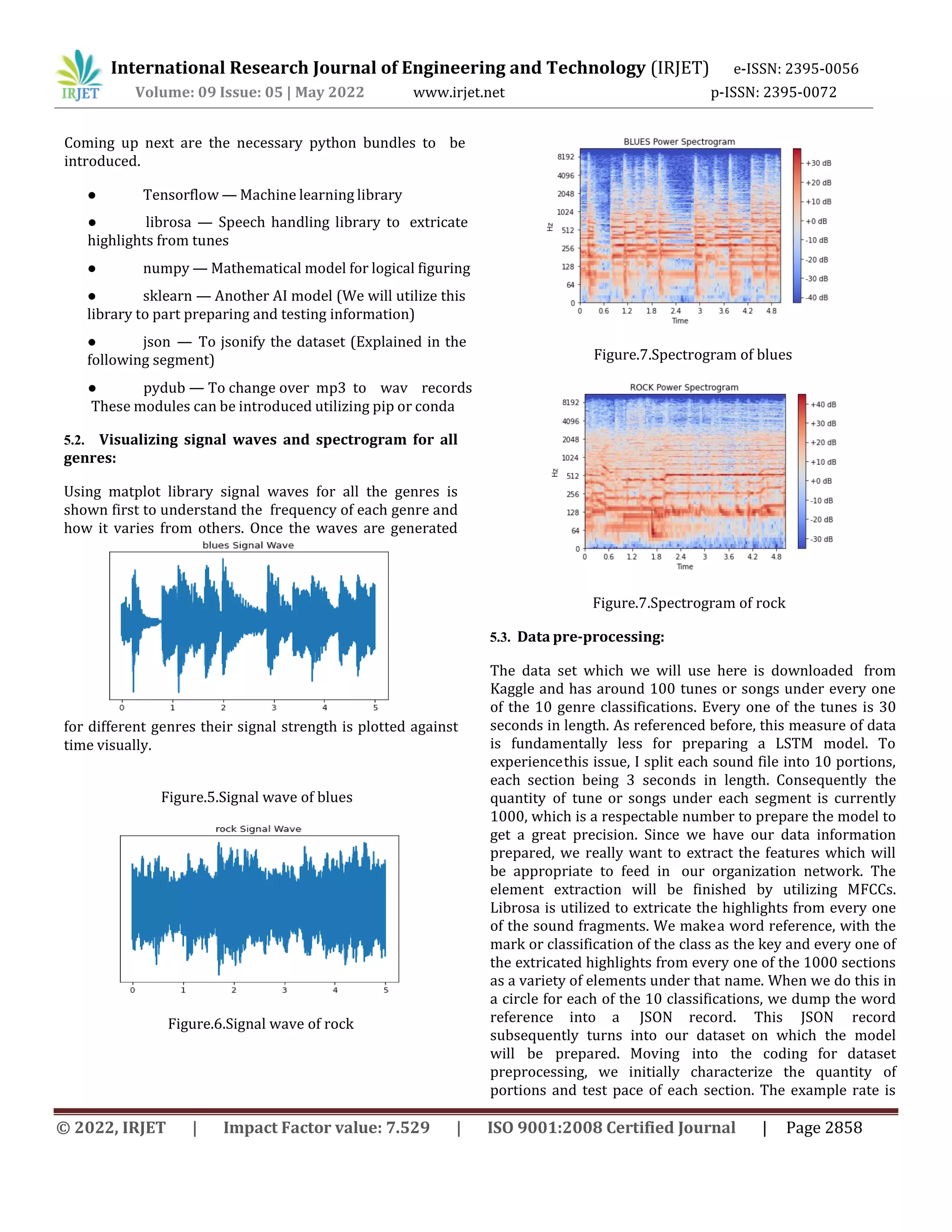
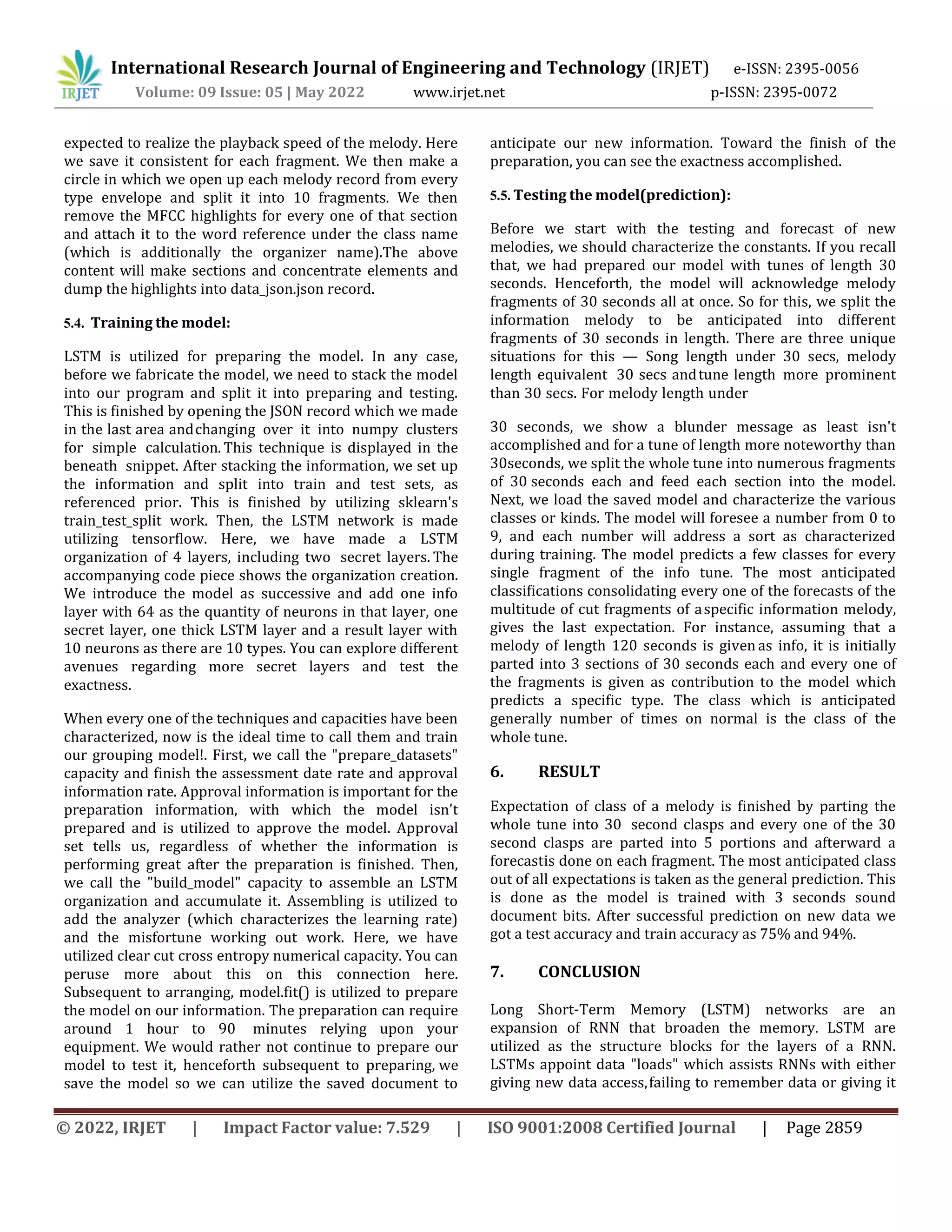
Volume: 09 Issue: 05 | May 2022 www.irjet.net p-ISSN: 2395-0072

Figure.1.Music representation in amplitude and time
Since this representation format doesn't provide much
information about the audio or the song, it uses something
called a Fast Fourier Transform (FFT) to represent the
audio in the frequency domain. FFT is a mathematical
algorithm that finds major applications in signal processing
used to transform the time domain into the frequency
domain. This FFT is used totransform the input audio file
and represent it in the frequency and time domains. A
graph that displays audio data in the frequency and time
domains is called a spectrogram, as shown.
Figure.2.Spectrogram(Audio data in frequency and time)
A spectrogram is a lot of FFTs stacked on top of one
another. It is an approach to outwardly address a sign's
tumult, or plentifulness, as it changes over the long run at
various frequencies. Here, the y axis is changed over
completely to a mel scale, and the variety aspect is
switched over completely todecibels (you can consider this
the log size of the sufficiency). This is done as people can
see a tiny and concentrated scope of frequencies and
amplitudes and the human ear chips away at the
guideline of a logarithmic scale. The ordinary spectrogram
can be utilized for extricating highlights, however this
actually contains some measure of extra data which isn't
needed. Since the human ear works on logarithms instead
of direct ones, we use chalk spectrograms that convert
these spectrograms into logarithmic portrayals for more
precise portrayal by eliminatingor disposing of undesirable
elements.
3.1. ADVANTAGES
To train the Tensor model and keras is used. The model
trained with RNN-LSTM algorithm should be made to run at
least for 50 epochs to obtain a train accuracy of 94% and
hence it will predict the genre correctly.
In this project almost 10 different genres are used for
prediction. Namely blues. classical, country, disco, hip hop,
jazz, metal, pop, reggae and rock.
4. ARCHITECTURE DIAGRAM
Figure.3.Workflow diagram of proposed model
Figure.4.Entity relationship diagram for the proposed model
5.1. Installing required packages:
There are a couple of modules which will be expected to be
introduced in your PC/PC to begin. We will construct the
wholeLSTM model utilizing Tensorflow, coded in python. We
will beworking with python 3.6 or higher (python 3.6 version
or aboveis expected to use).
5. EXPERIMENTS

● Tensorflow — Machine learning library
● numpy — Mathematical model for logical figuring
● sklearn — Another AI model (We will utilize this
library to part preparing and testing information)
● json — To jsonify the dataset (Explained in the
following segment)
5.2. Visualizing signal waves and spectrogram for all
genres:
Using matplot library signal waves for all the genres is
shown first to understand the frequency of each genre and
how it varies from others. Once the waves are generated
for different genres their signal strength is plotted against
time visually.
Figure.5.Signal wave of blues
Figure.6.Signal wave of rock
Figure.7.Spectrogram of blues
Figure.7.Spectrogram of rock
5.3. Data pre-processing:
The data set which we will use here is downloaded from
Kaggle and has around 100 tunes or songs under every one
of the 10 genre classifications. Every one of the tunes is 30
seconds in length. As referenced before, this measure of data
is fundamentally less for preparing a LSTM model. To
experiencethis issue, I split each sound file into 10 portions,
each section being 3 seconds in length. Consequently the
quantity of tune or songs under each segment is currently
1000, which is a respectable number to prepare the model to
get a great precision. Since we have our data information
prepared, we really want to extract the features which will
be appropriate to feed in our organization network. The
element extraction will be finished by utilizing MFCCs.
Librosa is utilized to extricate the highlights from every one
of the sound fragments. We makea word reference, with the
mark or classification of the class as the key and every one of
the extricated highlights from every one of the 1000 sections
as a variety of elements under that name. When we do this in
a circle for each of the 10 classifications, we dump the word
reference into a JSON record. This JSON record
subsequently turns into our dataset on which the model
will be prepared. Moving into the coding for dataset
preprocessing, we initially characterize the quantity of
portions and test pace of each section. The example rate is
● librosa — Speech handling library to extricate
highlights from tunes
● pydub — To change over mp3 to wav records
These modules can be introduced utilizing pip or conda
Coming up next are the necessary python bundles to be
introduced.

expected to realize the playback speed of the melody. Here
we save it consistent for each fragment. We then make a
circle in which we open up each melody record from every
type envelope and split it into 10 fragments. We then
remove the MFCC highlights for every one of that section
and attach it to the word reference under the class name
(which is additionally the organizer name).The above
content will make sections and concentrate elements and
dump the highlights into data_json.json record.
5.4. Training the model:
LSTM is utilized for preparing the model. In any case,
before we fabricate the model, we need to stack the model
into our program and split it into preparing and testing.
This is finished by opening the JSON record which we made
in the last area andchanging over it into numpy clusters
for simple calculation. This technique is displayed in the
beneath snippet. After stacking the information, we set up
the information and split into train and test sets, as
referenced prior. This is finished by utilizing sklearn's
train_test_split work. Then, the LSTM network is made
utilizing tensorflow. Here, we have made a LSTM
organization of 4 layers, including two secret layers. The
accompanying code piece shows the organization creation.
We introduce the model as successive and add one info
layer with 64 as the quantity of neurons in that layer, one
secret layer, one thick LSTM layer and a result layer with
10 neurons as there are 10 types. You can explore different
avenues regarding more secret layers and test the
exactness.
When every one of the techniques and capacities have been
characterized, now is the ideal time to call them and train
our grouping model!. First, we call the "prepare_datasets"
capacity and finish the assessment date rate and approval
information rate. Approval information is important for the
preparation information, with which the model isn't
prepared and is utilized to approve the model. Approval
set tells us, regardless of whether the information is
performing great after the preparation is finished. Then,
we call the "build_model" capacity to assemble an LSTM
organization and accumulate it. Assembling is utilized to
add the analyzer (which characterizes the learning rate)
and the misfortune working out work. Here, we have
utilized clear cut cross entropy numerical capacity. You can
peruse more about this on this connection here.
Subsequent to arranging, model.fit() is utilized to prepare
the model on our information. The preparation can require
around 1 hour to 90 minutes relying upon your
equipment. We would rather not continue to prepare our
model to test it, henceforth subsequent to preparing, we
save the model so we can utilize the saved document to
anticipate our new information. Toward the finish of the
preparation, you can see the exactness accomplished.
5.5. Testing the model(prediction):
Before we start with the testing and forecast of new
melodies, we should characterize the constants. If you recall
that, we had prepared our model with tunes of length 30
seconds. Henceforth, the model will acknowledge melody
fragments of 30 seconds all at once. So for this, we split the
information melody to be anticipated into different
fragments of 30 seconds in length. There are three unique
situations for this — Song length under 30 secs, melody
length equivalent 30 secs andtune length more prominent
than 30 secs. For melody length under
30 seconds, we show a blunder message as least isn't
accomplished and for a tune of length more noteworthy than
30seconds, we split the whole tune into numerous fragments
of 30 seconds each and feed each section into the model.
Next, we load the saved model and characterize the various
classes or kinds. The model will foresee a number from 0 to
9, and each number will address a sort as characterized
during training. The model predicts a few classes for every
single fragment of the info tune. The most anticipated
classifications consolidating every one of the forecasts of the
multitude of cut fragments of aspecific information melody,
gives the last expectation. For instance, assuming that a
melody of length 120 seconds is given as info, it is initially
parted into 3 sections of 30 seconds each and every one of
the fragments is given as contribution to the model which
predicts a specific type. The class which is anticipated
generally number of times on normal is the class of the
whole tune.
6. RESULT
Expectation of class of a melody is finished by parting the
whole tune into 30 second clasps and every one of the 30
second clasps are parted into 5 portions and afterward a
forecastis done on each fragment. The most anticipated class
out of all expectations is taken as the general prediction. This
is done as the model is trained with 3 seconds sound
document bits. After successful prediction on new data we
got a test accuracy and train accuracy as 75% and 94%.
7. CONCLUSION
Long Short-Term Memory (LSTM) networks are an
expansion of RNN that broaden the memory. LSTM are
utilized as the structure blocks for the layers of a RNN.
LSTMs appoint data "loads" which assists RNNs with either
giving new data access,failing to remember data or giving it

significance enough to affect the result. The model predicts
a few kinds for every single portion of the input tune. The
most anticipated music genre joining every one of the
predictions of the relative multitude of cut sections of a
specific input tune, gives the last prediction. For instance,
on the off chance that a tune of length 120 seconds is given
as information, it is initially parted into 3 fragments of 30
seconds each and every one of the sections is given as
contribution to the model which predicts a specific kind.
The genre which is anticipated generally number of times
on normal is the genre of the whole tune or song.
8. REFERENCES
[1] A. Meng, P. Ahrendt, J. Larsen, and L. K. Hansen,
“Temporal feature integration for music genre
classification,” Audio, Speech, and Language Processing,
IEEE Transactions on, vol. 15, no. 5, pp. 1654–1664, 2007.
[2] K. He and J. Sun, ‘‘Convolutional neural networks at
constrained time cost,’’ in Proc. IEEE Conf. Comput. Vis.
Pattern Recognit. (CVPR), Jun. 2015, pp. 5353–5360.
[3] I. H. Chung, T. N. Sainath, B. Ramabhadran, M. Picheny, J.
Gunnels, V. Austel, U. Chauhari, and B. Kingsbury, “Parallel
deep neural network training for big data on blue gene/q,”
in Proceedings of the International Conference for High
Performance Computing, Networking, Storage and
Analysis, 2015, pp. 745–753.
[4] David Opitz and Richard Maclin, Popular Ensemble
Methods: An Empirical Study, Journal of Artificial
IntelligenceResearch 11, 1999, pp. 169-198.
[5] Y. Song and C. Zhang, “Content-based information fusion
for semi-supervised music genre classification,”
Multimedia, IEEE Transactions on, vol. 10, no. 1, pp. 145–
152, 2008.
[6] Piero Baraldi, Enrico Zio , Davide Roverso , Feature
Selection For Nuclear Transient Diagnostics, OECD Halden
Reactor Project, January 2007.

FORECASTING MUSIC GENRE (RNN - LSTM)

More Related Content

Similar to FORECASTING MUSIC GENRE (RNN - LSTM)

More from IRJET Journal

Recently uploaded

FORECASTING MUSIC GENRE (RNN - LSTM)