Recognition of music genres using deep learning.

© 2022, IRJET | Impact Factor value: 7.529 | ISO 9001:2008 Certified Journal | Page 936
Recognition of music genres using deep learning.
Vishal Phulmante1, Ambar Bidkar2, Yashkumar Mundada3, Mrs. Prutha P. Kulkarni4
1,2,3Department of Electronics & Tele-Communication Engineering,
Vishwakarma Institute of Information Technology Pune, Maharashtra, India.
4Asst. Professor,Department of Electronics & Tele-Communication Engineering,
Vishwakarma Institute of Information Technology Pune, Maharashtra, India.
---------------------------------------------------------------------***---------------------------------------------------------------------
Abstract - The paper encapsulates recognition of music
genres by using convolution neural networks (CNNs). Three
different approaches were considered for implementing the
solution to the problem. The first approach is to extract Mel-
spectrograms , second one is to extract MFCC plots and the
last one is by plotting chroma STFT features of the audio
files. The aim of this project work is to test the different
audio features which are best suitable for such kinds of
tasks.
Key Words: Music Genre Recognition, Audio
Processing, Deep Learning, Convolution Neural
Networks, Mel-spectrograms, Mel Frequency Cepstral
Coefficients, Chroma STFT.
1. INTRODUCTION
Music information retrieval (MIR) is a field that
incorporates components of machine learning, signal
processing and music theory to study the musical content
present in the audio sample. MIR allows machine
algorithms to smartly analyze and process data present in
the given music sample[3]. The music consumption is
increasing day by day due to the ever increasing platforms
for music and music stores i.e databases and new music
creation. Users find it difficult to organize songs which
they listen to. Genre, which is determined by various
aspects in the music sample such as rhythms, harmonic
information, and instruments which are used in that
particular music, is a way to differentiate and group songs
together[1].
Developing a system capable of segregating music
genres, indirectly through audio is very challenging. The
basic objective is to recognize music genres on the basis of
audio provided and perform relatively well. The model can
identify music genres with higher accuracy on the unseen
data.
2. LITERATURE STUDY
In the paper titled “Convolutional Neural Network
Achieves Human-level Accuracy in Music Genre
Classification''[10] authors used CNN model having two
convolution layers with Mel-spectrogram features which
in turn gave them an accuracy of around 70%. They split
the audio files into smaller chunks of 3sec length.
The authors of the paper “Music genre classification
looking for the Perfect Network?”[11] worked on different
architectures like CNN, CRNN and LSTM. They got the
highest accuracy of 52% with a CNN model using Mel-
spectrograms as an input.
Athulya K M and Sindhu S in their work titled “In Deep
learning-based music genre classification using
spectrogram”[12] got an impressive accuracy of around
94% using a CNN model having 5 convolution 2D layers
with Mel-spectrogram features.
The authors of “Deep attention based music genre
classification” proposed the GRU based Bidirectional
Recurrent Neural Network architecture[13]. They got an
overall accuracy of 92.7% on the GTZAN dataset.
3. METHODOLOGY
There are mainly four different steps are involved in
the proposed work:
1. Data collection
2. Data preprocessing
3. Feature extraction
4. Genre Classification
Fig-1: Process Workflow
3.1 Data Collection
GTZAN genre dataset has been used in this process.
The GTZAN dataset is the widely used public dataset for
evaluation in deep listening research for music genre
recognition (MGR) tasks[4].
The dataset consists of 100 audio tracks for each of 10
genres. The audio files are 30 sec long 22050Hz Mono 16-
bit in .wav format. The 10 different genres can be seen in
table-1.
International Research Journal of Engineering and Technology (IRJET) e-ISSN: 2395-0056
Volume: 09 Issue: 05 | May 2022 www.irjet.net p-ISSN: 2395-0072

Genres present in the dataset
Classic Country Blues Jazz Pop
Rock Metal Reggae Disco HipHop
Table-1: Genres present in GTZAN dataset
3.2 Data Preprocessing
Before extracting the features the audio files need to be
split into 3sec long smaller chunks so as to avoid the
clustered feature plots. If the audio files are not split, the
visual representation of these audio files in frequency-
time domain could be inconsistent and can overwhelm the
CNN model to learn the features from it.
For splitting the audio files the librosa python library is
used along with the soundfile library for saving the audio
files once they are split.
The splitting of the audio files led to the generation of ten
files from one. Ten audio files of the Jazz genre were
smaller than 30sec length so they yielded 10 samples less
than other genres. Now the dataset contains 9990 samples
for 10 genres.
The dataset is then split into 4:1 ratio for training and
testing the model respectively.
o Training data : 8000 samples
o Test data : 1990 samples
3.3 Feature Extraction
Once the data preprocessing is done, the audio features
are now extracted from audio files. The features like Mel-
spectrograms, MFCCs and Chroma STFT are taken using
the librosa library. Librosa is a python library especially
designed for audio processing. Its pre-built functions allow
us to extract the audio features at much ease[5][6][9].
3.3.1 Mel-Spectrograms
Spectrograms are images that represent the frequency
content of a signal which varies with time. In a
spectrogram the X-axis represents time, Y-axis represents
frequency and the third dimension in the spectrogram
represents the amplitude or intensity of a particular
frequency value at a particular given time in a color coded
format[5]. The spectrograms of 1440 x 720 pixels were
extracted from the audio file. The samples can be seen in
fig-2 and fig-3.
o No. of mels : 250
o Number of FFT : 1024
o Hop length : 256
o Window length : 1024
o Window Type : Hanning
Fig-2: Mel-spectrogram of Blues genre
Fig-3: Mel-spectrogram of Disco genre
3.3.2 Mel-Frequency Cepstral Coefficients (MFCCs)
Mel Frequency Cepstral Coefficient feature extraction
method is Widely used in speech recognition domain.
MFCC Keeps only linguistic features and discards
unimportant things. MFC is an illustration of a sound’s
short-term power spectrum based on a linear cosine
transform of a log power spectrum on a nonlinear mel
scale of frequency which is used in sound processing for
feature extraction[9]. MFCCs are derived by fourier
transform of the windowed portion of a signal and map
the powers of these spectrums onto the mel scale using
triangular overlappings or cosine overlapping windows.
Log of the power is taken at each of the mel
frequencies[5][6]. Then at last DCT of the list of mel log
powers is taken, the amplitudes of the final spectrum are
MFCCs. Figure 4. showcases the above MFCC extraction
flow. Steps involved in extracting MFCCs:
1) Frame signal into short frames and apply
windowing like Hanning.
2) For each frame, find its spectral density by
characterizing it in the frequency domain.
3) Apply the Mel filterbank to above power spectra,
sum the energy in each filter.
4) Take logarithm of all the filterbank energies.
5) Take DCT of the log filterbank energies.
Fig-4: Block diagram of MFCCs extraction process

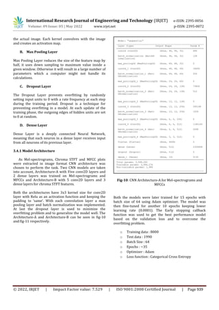
o Number of MFCCs = 13
o Number of FFT = 1024
o Hop length = 256
Since CNN architecture has been chosen, plotting these
MFCC’s is necessary. By using the librosa library these
MFCC’s were plotted into logarithmic scale as can be seen
in fig-5 and fig-6.
Fig-5: MFCC Plot of Blues genre
Fig-6: MFCC Plot of Disco genre
3.3.3 Chroma STFT
The chroma values represent the intensity of the
twelve different pitch classes which are used in music
research. Chroma STFT uses short-term Fourier
transformation to determine Chroma features[8].
STFT represents the classification information of pitch
and signal structure present in the audio sample. An
important characteristic of the chroma function is to
capture the overtone and tune characteristics of the
music.[7][9].
o n_chroma = 12
o n_fft = 4096
o Hop length = 256
o Window = hanning
Various Pitch classes
C C# D D# E F
F# G G# A A# B
Table-2: Twelve Pitch classes present in chroma STFT
The samples of chroma STFT plots can be seen in fig-7 and
fig-8 for blues and disco genres respectively.
Fig-7: Chroma STFT Plot of Blues genre
Fig-8: Chroma STFT Plot of Disco genre
3.4 Genre Classification
Once the audio features are extracted, now it's time to
build a suitable deep learning model. There is a huge room
for tweaks to current existing models.
There are mainly three classes of neural networks,
Multilayer Perceptrons (MLP), Convolutional Neural
Networks (CNN) and Recurrent Neural Networks (RNN).
Convolutional Neural Networks or CNN are built to map
data from images and assign it to an output variable for
further processing. This method has proven effective on
image data as an input. CNN is extensively used in Image
related problems, classification and regression related
problems. Figure-9 explains the working flow of a CNN
architecture.
Fig-9: Typical CNN architecture
A. Convolution Layer
A convolutional layer is the main building block of a CNN
architecture. It comprises multiple kernels, parameters of
which are to be learned throughout the training process.
The size of these kernels is usually smaller ( 3 x 3 ) than

the actual image. Each kernel convolves with the image
and creates an activation map.
B. Max Pooling Layer
Max Pooling Layer reduces the size of the feature map by
half, it uses down sampling to maximum value inside a
given window. Otherwise it will result in a large number of
parameters which a computer might not handle its
calculations.
C. Dropout Layer
The Dropout Layer prevents overfitting by randomly
setting input units to 0 with a rate frequency at each step
during the training period. Dropout is a technique for
preventing overfitting in a model. At each update of the
training phase, the outgoing edges of hidden units are set
to 0 at random.
D. Dense Layer
Dense Layer is a deeply connected Neural Network,
meaning that each neuron in a dense layer receives input
from all neurons of its previous layer.
3.4.1 Model Architecture
As Mel-spectrograms, Chroma STFT and MFCC plots
were extracted in image format CNN architecture was
chosen to perform the task. Two CNN models are taken
into account, Architecture-A with Five conv2D layers and
2 dense layers was trained on Mel-spectrograms and
MFCCs and Architecture-B with 5 conv2D layers and 3
dense layers for chroma STFT features.
Both the architectures have 3x3 kernel size for conv2D
layer with Relu as an activation function and keeping the
padding to ‘same’. With each convolution layer a max
pooling layer and batch normalization was implemented.
At last the dropout layer is used to minimize the
overfitting problem and to generalize the model well. The
Architecture-A and Architecture-B can be seen in fig-10
and fig-11 respectively.
Fig-10: CNN Architecture-A for Mel-spectrograms and
MFCCs
Both the models were later trained for 15 epochs with
batch size of 64 using Adam optimizer. The model was
then fine-tuned for another 10 epochs keeping lower
learning rate (0.0001). The Early stopping callback
function was used to get the best performance model
based on the validation loss and to overcome the
overfitting problem.
o Training data : 8000
o Test data : 1990
o Batch Size : 64
o Epochs : ~35
o Optimizer : Adam
o Loss function : Categorical Cross Entropy

Fig-11: CNN Architecture-B for Chroma STFT features
4. RESULTS
The CNN Architecture-A model performed really
well with Mel-spectrograms as an input having an
accuracy of over 90%. Second best model was with MFCC
audio features giving above 70% accuracy. The CNN
Architecture-B with Chroma STFT features was least
promising with an accuracy of just 57%. This work
showcases the effectiveness of Mel-Spectrograms for the
genre classification task.
The detailed performance of the three audio
features for the test dataset can be seen in the below
confusion matrices and classification reports.
Feature Accuracy Support
Spectrogram 91% 1990
MFCC 72% 1990
Chroma STFT 57% 1990
Table-3: Performance of Audio features
Fig-12: Confusion matrix of mel-spectrogram model on
test dataset
Fig-13: Classification report of mel-spectrogram model on
test dataset

Fig-14: Confusion matrix of MFCC model on test dataset
Fig-15: Classification report of MFCC model on test
dataset
Fig-16: Confusion matrix of Chrome STFT model on test
dataset
Fig-17: Classification report of Chroma STFT model on
test dataset
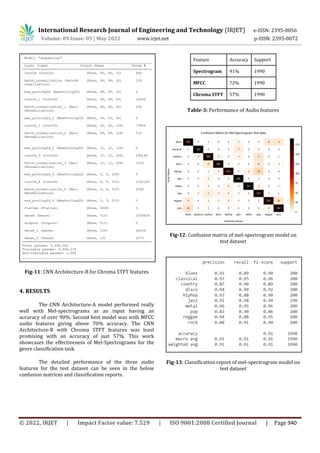
5. CONCLUSION
From the confusion matrices and classification
reports it can be concluded that Mel-spectrograms are
very effective audio features for the classification tasks.
While the mel-spectrogram model was able to classify all
genres with over 90% accuracy, the MFCC and Chroma
STFT models struggled to maintain even 70% accuracy for
different genres.
Although the MFCC model performed decently on
most of the genres, it was having a hard time classifying
the Rock genre with just 47% accuracy. Chroma STFT
features were found to be least promising among the other
two features.
6. FUTURE WORK
For future work the dataset can be tested on the
different neural network architectures like RCNN, BRNN
and more. Moving ahead even more audio features like
Zero Crossing Rate, Spectral Rolloff, Zooming in, Spectral
centroid and more can be taken into consideration for
performing this task.
REFERENCES
[1] Li, T., Ogihara, M., & Li, Q. (2003). A Comparative
Study on Content-Based Music Genre Classification.
SIGIR Forum (ACM Special Interest Group on
Information Retrieval), (SPEC. ISS.), 282-289.
https://doi.org/10.1145/860484.860487
[2] A. Meng, P. Ahrendt, J. Larsen and L. K. Hansen,
"Temporal Feature Integration for Music Genre
Classification," in IEEE Transactions on Audio, Speech,
and Language Processing, vol. 15, no. 5, pp. 1654-
1664, July 2007, doi: 10.1109/TASL.2007.899293.

[3] Hindawi Publishing Corporation EURASIP Journal on
Advances in Signal Processing Volume 2007, Article ID
36409, 8 pages doi:10.1155/2007/36409
[4] Bahuleyan, H., 2018. Music genre classification using
machine learning techniques. arXiv preprint
arXiv:1804.01149.
[5] Haggblade, M., Hong, Y. and Kao, K., 2011. Music genre
classification. Department of Computer Science,
Stanford University doi=10.1.1.375.204
[6] Y.M.G. Costa, L.S. Oliveira, A.L. Koerich, F. Gouyon, J.G.
Martins, Music genre classification using LBP textural
features, Signal Processing, Volume 92, Issue 11, 2012,
Pages 2723-2737, ISSN 0165-1684,
https://doi.org/10.1016/j.sigpro.2012.04.023.
[7] Music genre classification and music recommendation
by using deep learning A. Elbir and N. Aydin
ELECTRONICS LETTERS 11th June 2020 Vol. 56 No.
12 pp. 627–629
[8] L. Shi, C. Li and L. Tian, "Music Genre Classification
Based on Chroma Features and Deep Learning," 2019
Tenth International Conference on Intelligent Control
and Information Processing (ICICIP), 2019, pp. 81-86,
doi: 10.1109/ICICIP47338.2019.9012215.
[9] G. Tzanetakis and P. Cook, "Musical genre
classification of audio signals," in IEEE Transactions
on Speech and Audio Processing, vol. 10, no. 5, pp.
293-302, July 2002, doi: 10.1109/TSA.2002.800560.
[10] Dong, M., 2018. Convolutional neural network
achieves human-level accuracy in music genre
classification. arXiv preprint arXiv:1802.09697.
[11] Kostrzewa, D., Kaminski, P. and Brzeski, R., 2021, June.
Music Genre Classification: Looking for the Perfect
Network. In the International Conference on
Computational Science (pp. 55-67). Springer, Cham.
[12] K M, Athulya and S, Sindhu, Deep Learning Based
Music Genre Classification Using Spectrogram (July
10, 2021). Proceedings of the International
Conference on IoT Based Control Networks &
Intelligent Systems - ICICNIS 2021, SSRN:
https://ssrn.com/abstract=3883911 or
http://dx.doi.org/10.2139/ssrn.3883911
[13] Yu, Y., Luo, S., Liu, S., Qiao, H., Liu, Y. and Feng, L., 2020.
Deep attention based music genre classification.
Neurocomputing, 372, pp.84-91.

Recognition of music genres using deep learning.

More Related Content

Similar to Recognition of music genres using deep learning.

More from IRJET Journal

Recently uploaded

Recognition of music genres using deep learning.