IRJET- Music Genre Classification using Machine Learning Algorithms: A Comparison

International Research Journal of Engineering and Technology (IRJET) e-ISSN: 2395-0056
Volume: 06 Issue: 05 | May 2019 www.irjet.net p-ISSN: 2395-0072
© 2019, IRJET | Impact Factor value: 7.211 | ISO 9001:2008 Certified Journal | Page 851
Music Genre Classification using Machine Learning Algorithms: A
comparison
Snigdha Chillara1, Kavitha A S2, Shwetha A Neginhal3, Shreya Haldia4, Vidyullatha K S5
1,2,3,4,5Department of Information Science and Engineering,
Dayananda Sagar College of Engineering, Bangalore– 560078, Karnataka, India
---------------------------------------------------------------------***---------------------------------------------------------------------
Abstract - Music plays a very important role in people’s
lives. Music bring like-minded people together and is the glue
that holds communities together. Communities can be
recognized by the type of songs that they compose, or even
listen to. The purpose of our project and research is to find a
better machine learning algorithm than the pre-existing
models that predicts the genre of songs. In this project, we
built multiple classification models and trained them over the
Free Music Archive (FMA) dataset. We have compared the
performances of all these models and logged their results in
terms of prediction accuracies. Few of these models are
trained on the mel-spectrograms of the songs along with their
audio features, and few others are trained solely on the
spectrograms of the songs. It is found that one of the models, a
convolutional neural network, which was given just the
spectrograms as the dataset, has given the highest accuracy
amongst all other models.
Key Words: Music Information Retrieval, spectrograms,
neural networks, feature extraction, classification
1. INTRODUCTION
Sound is represented in the form of an audio signal having
parameters like frequency, decibel, bandwidth etc. A typical
audio signal can be expressed as a functionofAmplitudeand
Time. These audio signals come in various different formats
which make it possible and easy for the computer to read
and analyze them. Some formats are: mp3 format, WMA
(Windows Media Audio) format and wav (Waveform Audio
File) format.
Companies (such as Soundcloud, Apple Music,
Spotify, Wynk etc) use music classification, either to place
recommendations to their customers, or simplyasa product
(like Shazam). To be able to do any of the above two
mentioned functions, determining music genres is the first
step. To achieve this, we can take the help of Machine
Learning algorithms. These machine learning algorithms
prove to be very handy in Music Analysis too.
Music Analysis is done based on a song’s digital
signatures forsomefactors,includingacoustics,danceability,
tempo, energy etc., to determine the kind of songs that a
person is interested to listen to.
Music is characterized by giving them categorical labels
called genres. These genres are created by humans. A music
genre is segregated by the characteristics which are
commonly shared by its members. Typically, these
characteristics are related to the rhythmic structure,
instrumentation, and the harmonic content of the music. To
categorize music files into their respectivegenres,itisa very
challenging task in the area of Music Information Retrieval
(MIR), a field concerned with browsing, organizing and
searching large music collections.
Classification of genre can be very valuable to explain
some interesting problems such as creating songreferences,
tracking down related songs, discovering societies that will
like that specific song, sometimes it can also be used for
survey purposes.
Automatic musical genre classification can assist
humans or even replace them inthisprocessandwould beof
a very valuable addition to music information retrieval
systems. In addition to this, automatic classificationofmusic
into genres can provide a framework for development and
evaluation of features for any type of content-basedanalysis
of musical signals
The concept of automatic music genre classification has
become very popular in recent years as a result of the rapid
growth of the digital entertainment industry.
Dividing music into genres is arbitrary, but there are
perceptual criteria that are related to instrumentation,
structure of the rhythm and texture of the music that can
play a role in characterizing particular genre. Until now
genre classification for digitally available music has been
performed manually. Thus, techniques for automatic genre
classification would be a valuable addition to the
development of audio information retrieval systems for
music.
1.1 Problem Statement
Music plays a very important role in people’s lives. Music
bring like-minded people together and is the glue that holds
communities together. Communities can be recognized by
the type of songs that they compose, or even listen to.
Different communities and groups listentodifferentkindsof
music. One main feature that separates one kind of music
from another is the genre of the music.
The aim of this project is:

1. To build a machine learning model which classifies
music into its respective genre.
2. To compare the accuracies of this machinelearning
model and the pre-existing models, and draw the necessary
conclusions.
1.2 Objectives
1. Developing a machine learning model thatclassifies
music into genres shows that there exists a solution which
automatically classifies music into its genres based on
various different features, instead of manually entering the
genre.
2. Another objective is to reach a good accuracy so that the
model classifies new music into its genre correctly
3. This model should be better than at least a few pre-
existing models.
2. RELATED WORK
Some works published in last two years show that
investigations related to musical genre in music information
retrieval scenario are not exhausted, and they still remainas
an active research topic, as one can note in the following:
I. In Hareesh Bahuleyan, (2018). Music Genre
Classification using Machine Learning techniques, the
work conducted gives an approach to classify music
automatically by providing tags to the songs present in the
user’s library. It explores both Neural Network and
traditional method of using Machine Learning algorithms
and to achieve their goal. The first approach uses
Convolutional Neural Network which is trained end to end
using the features of Spectrograms (images) of the audio
signal. The second approach uses various Machine Learning
algorithms like Logistic Regression, Random forest etc,
where it uses hand-crafted features from time domain and
frequency domain of the audio signal. The manually
extracted features like Mel-Frequency Cepstral Coefficients
(MFCC), Chroma Features, Spectral Centroid etc are used to
classify the music into its genres using ML algorithms like
Logistic Regression, Random Forest, Gradient Boosting
(XGB), Support Vector Machines (SVM). By comparing the
two approaches separately they came to a conclusion that
VGG-16 CNN model gave highest accuracy. By constructing
ensemble classifier of VGG-16 CNN and XGB the optimised
model with 0.894 accuracy was achieved.
II. In Tzanetakis G. et al., (2002). Musical genre
classification of audio signals, they have mainly explored
about how the automatic classificationofaudiosignalsintoa
hierarchy of musical genres is to be done. They believe that
these music genres are categorical labels that are created by
humans just to categorise pieces of music. They are
categorised by some of the common characteristics. These
characteristics are typically related to the instruments that
are used, the rhythmic structures, and mostly the harmonic
music content. Genre hierarchies are usually used to
structure the very large music collections which is available
on web. They have proposed three feature sets: timbral
texture, the rhythmic content and the pitch content. The
investigation of proposed features in order to analyse the
performance and the relative importance was done by
training the statistical pattern recognition classifiers by
making use of some real-world audio collections. Here, in
this paper, both whole file and the real time frame-based
classification schemes are described. Using the proposed
feature sets, this model can classify almost 61% of tenmusic
genre correctly.
III. In Lu L. et al., (2002). Content analysis for audio
classification andsegmentation,theyhavepresentedtheir
study of segmentation and classification of audio content
analysis. Here an audio stream is segmented according to
audio type or speaker identity. Their approach is to build a
robust model which is capable of classifying andsegmenting
the given audio signal into speech, music, environment
sound and silence. This classification is processed in two
major steps, which has made it suitable for various other
applications as well. The first step is speech and non-speech
discrimination. In here, a novel algorithm which is based on
KNN (K- nearest- neighbour)andlinearspectral pairs-vector
quantization (LSP-VQ) is been developed. The secondstepis
to divide the non-speech class into music, environmental
sounds, and silence with a rule- based classification method.
Here they have made use of few rare and new features such
as noise frame ratio, band periodicity which are not just
introduced, but discussed in detail. They have also included
and developed a speaker segmentation algorithm. This is
unsupervised. It uses a novel scheme based on quasi - GMM
and LSP correlation analysis. Without any prior knowledge
of anything, the model can support the open-set speaker,
online speaker modelling and also the real time
segmentation.
IV. In Tom LH Li et al., (2010). Automatic musical
pattern feature extraction using convolutional
neural network, they made an effort to understand the
main features which actually contribute to build the optimal
model for Music Genre Classification. The main purpose of
this paper is to propose a novel approach to extract musical
pattern features of the audio file using Convolution Neural
Network (CNN). Their core objective is to explore the
possibilities of application of CNN in Music Information
Retrieval (MIR). Their results and experiments show that
CNN has the strong capacity to capture informative features
from the varying musical pattern. The features extracted
from the audio clips such as statistical spectral features,
rhythm and pitch are lessreliableandproduceslessaccurate
models. Hence, the approach made by them to CNN, where
the musical data have similar characteristics to image data
and mainly it requires very less prior knowledge. The
dataset considered was GTZAN. It consists of 10 genres with
100 audio clips each. Each audio clip is 30 seconds,sampling

rate 22050 Hz at 16 bits. The musical patterns were
evaluated using WEKA tool where multiple classification
models were considered. The classifier accuracy was 84 %
and eventually got higher. In comparison to the MFCC,
chroma, temp features, the features extracted by CNN gave
good results and was more reliable. The accuracy canstill be
increased by parallel computing on different combinationof
genres.
3. DATASET
We make use of a subset of the Free Music Archive dataset
[FMA paper link], an open and easily accessible database of
songs that are helpful in evaluating several tasks inMIR.The
subset is called fma_small,a balanceddatasetwhichcontains
audio from 8000 songs arranged in a hierarchical taxonomy
of 8 genres. It provides 30 seconds length of high-quality
audio, pre-computed features, together with track-level and
user-level metadata, tags and free-form text such as
biographies.
The number of audio clips in each category has been
tabulated in Table1. Each audio file is about 1 megabyte,
hence the entire fma_small dataset is about 8 GB. There are
other variants of FMA dataset available too, as shown in
Table 2, which are the fma_mediumdataset(25,000tracksof
30s, 16 unbalanced genres (23 GiB)), fma_large dataset
(106,574 tracks of 30s, 161 unbalanced genres (98 GiB),
fma_full dataset (106,574 tracks of 30s, 161 unbalanced
genres (917 GiB)).
The dataset also provides a metadata thatallowstheusersto
experiment without dealing with feature extraction. These
are all the features the librosa Python library, version 0.5.0
was able to extract. Each feature set (except zero-crossing
rate) is computed on windows of 2048 samples spaced by
hops of 512 samples. Seven statistics were then computed
over all windows: the mean, standard deviation, skew,
kurtosis, median, minimum and maximum. Those 518 pre-
computed features are distributedinfeatures.csv (presentin
the fma metadata) for all tracks.
Other datasets that are open source and freely available
are shown in the Table 3
4. METHODOLOGY
This section gives the detailsofdata pre-processingfollowed
by a description about the proposed approach to this
classification problem.
4.1 Deep Neural Networks
With deep learning algorithms, we can achieve the task of
music genre classification without hand-crafted features.
Convolutional neural networks (CNNs) prove to be a great
choice for classifying images. The 3-channel (R-G-B) matrix
of an image is given to a CNN which then trains itself on
those images. In this study, the sound wave can be
represented as a spectrogram, which can be treated as an
image (Nanni et al., [4]) (Lidy and Schindler, [15]). The
task of the CNN is to use the spectrogram to predict the
genre label (one of eight classes).
S.No Genre Name Count
1 Electronic 1000
2 Experimental 1000
3 Folk 1000
4 Hip-Hop 1000
5 Instrumental 1000
6 International 1000
7 Pop 1000
8 Rock 1000
Total 8000
Table -1: Number of instances in each genre class
dataset clips genres Length
[s]
Size
[
GiB]
Size
#days
small 8000 8 30 7.4 2.8
medium 25000 16 30 23 8.7
large 106574 161 30 98 37
full 106574 161 278 917 343
Table -2: Variants of FMA dataset
dataset #clips #artists year audio
GTZAN 1000 ~300 2002 yes
MSD 1,000,000 44745 2011 no
AudioSet 2,084,320 - 2017 no
Artist20 1413 20 2007 yes
AcousticBrainz 2,524,739 - 2017 no
Table -3: List of other audio datasets

4.1.1 Spectrogram Generation
A spectrogram is a 2D representation of a signal,havingtime
on the x-axis and frequency on the y-axis. In this study, each
audio signal was converted into a MEL spectrogram (having
MEL frequency bins on the y-axis). The parameters used to
generate the power spectrogram using STFT are listed
below:
 Sampling rate (sr) = 22050
 Window size (n_fft) = 2048
 Hop length = 512
 X_axis: time
 Y_axis: MEL
 Highest Frequency (f_max) = 8000
The spectrograms from each genre are shown in Figure 1.
Fig- 1: Sample spectrograms for 1 audio track from each
music genre
4.1.2 Convolutional Neural Networks
From Figure 2, we can see that there exist some
characteristic patterns in the spectrograms of the audio
signals belonging to different classes. Hence spectrograms
can be considered as ‘images’ and can be given as input to a
CNN. A rough framework of the CNN model is shown in
Figure 3.
4.1.2.1 Feed Forward Network
A CNN is a feed-forward network, that is, input examples are
fed to the network and transformed into an output; with
supervised learning, the output would be a label, a name
applied to the input. That is, they maprawdata tocategories,
recognizing patterns that may signal, for example, that an
input image should be labeled “folk” or “experimental”. A
feedforward network is trained on labeled images until it
minimizes the error it makes whenguessingtheircategories.
With the trained set of parameters (or weights, collectively
known as a model), the network sallies forth to categorize
data it has never seen. A trainedfeedforward network canbe
exposed to any random collection of photographs, and the
first photograph it is exposed to will not necessarily alter
how it classifies the second. Seeing spectrogram of a folk
song will not lead the net to perceive a spectrogram of an
experimental song next. That is, a feedforward network has
no notion of order in time, and the only input it considers is
the current example it has been exposed to. Feedforward
networks are amnesiacs regarding their recent past; they
remember nostalgically only the formative moments of
training.
Fig -2: CNN Framework
4.1.2.2 Operations Of CNN
Each block in a CNN consists of the following operations:
 Convolution: This step involves a matrix filter (say 3x3
size) that is moved over the input image which is of
dimension image width ximageheight.Thefilterisfirst
placed on the image matrix and then we compute an
element-wise multiplication between the filter and the
overlapping portion of the image, followed by a
summation to give a feature value.
 Pooling: This method is used to reduce the dimension of
the feature map obtained from the convolution step. By
max pooling with 2x2 window size, we only retain the
element with the maximum value among the 4 elements
of the feature map that are covered in this window. We
move this window across the feature map with a pre-
defined stride.
 Non-linear Activation: The convolution operation is
linear and in order to make the neural network more

powerful, we need to introduce some non-linearity. For
this purpose, we can apply an activation function such as
Rectifier Linear Unit (ReLU) on each element of the
feature map.
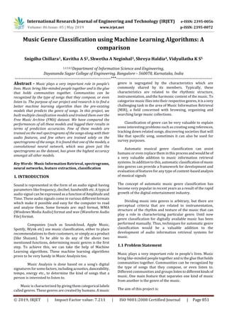
The model consists of 3 convolutional blocks (conv base),
followed by a flatten layer which converts a 2D matrix to a
1D array, which is then followed by a fully connected layer,
which outputs the probability that a given image belongs to
each of the possible classes.
The final layer of the neural network outputs the class
probabilities (using the softmaxactivationfunction)foreach
of the eight possible class labels. The cross-entropy loss is
computed as shown below:
where, M is the number of classes; yo,c is a binary indicator
whose value is 1 if observation o belongs to class c and 0
otherwise; po,c is the model’s predicted probability that
observation o belongs to class c. This loss is used to
backpropagate the error, computethegradientsandthereby
update the weights of the network. This iterative process
continues until the loss converges to a minimum value.
4.1.3 Convolutional Recurrent Neural Network
To compare the performance improvement that can be
achieved by the CNNs, we train a Convolutional Recurrent
Neural Network, which is a combination of convolutional
neural networks and recurrent neural networks.
4.1.3.1 Recurrent Neural Networks
Recurrent nets are a type of artificial neural network
designed to recognize patterns in sequences of data, such as
textual data, genomes, audio, video, or numerical times
series data emanating from sensors, stock markets and
government agencies. These algorithms take time and
sequence into account, they have a temporal dimension.
RNNs are applicable even to images, which can be
decomposed into a series of patches and treated as a
sequence.
Recurrent networksaredistinguishedfromfeedforward
networks by that feedback loop connected to their past
decisions, ingesting their own outputs moment after
moment as input. It is often said that recurrent networks
have memory. Adding memory to neural networks has a
purpose: There is information in the sequence itself, and
recurrent nets use it to perform tasks that feedforward
networks can’t.
Long Short-Term Memory networks – usuallyjustcalled
“LSTMs” – are a special kind of RNN, capable of learning
long-term dependencies. They were introduced by
Hochreiter & Schmidhuber (1997).
4.1.3.2 CRNN Model Details
The CNN-RNN model, shortly called as CRNN model has 3 1-
dimensional Convolution Layers followed by an LSTM layer
of the RNN, which is then followed by a fully connected
dense layer, which is the output layer. The batch size usedin
this model is 32, number of epochs is maintained as 30, to
keep the evaluation and comparison fair. The activation
function used is ReLU. To avoid overfitting of the data,
Dropout of 0.2 is implemented in the hidden layers.
4.1.4 CNN-RNN Parallel Model
This model runs the CNN model and the RNN model in
parallel, keeping all the metrics and regularization factors
the same as implemented in the previous models.Theidea is
to compare a simple CNN model with these robust, complex
models to assess the performance metrics and compare the
models.
4.1.5 Implementation Details
The spectrogram images have a dimension of 150 x 150. For
the feed-forward network connectedtotheconvbase,a 512-
unit hidden layer is implemented. Over-fitting is a common
issue in neural networks. In order to prevent this, we
adopted the following strategy:
Dropout [21]: This is a regularization mechanism in which
we shut-off some of the neurons (set their weights to zero)
randomly during training. In each iteration, we use a
different combination of neurons to predict the final output,
thereby randomizing the training cycles. A dropout rate of
0.2 is used, i.e., a given weight is set to zero during an
iteration, with a probability of 0.2.
The dataset is randomly split into training set (80%),
validation set (10%), testing set (10%). The same split is
used for all the comparisons.
The neural networks are implemented in Python using
Tensorflow. All models were trained for 30 epochs with a
batch size of 64. The optimizer used in these neural
networks was the ADAM optimizer. One epoch refers to one
iteration over the entire training set.
4.2 Feature Extraction
This section describes the features that have been extracted
for other models that are compared to the proposed model.
Features can be broadly classified as time domain and
frequency domain features. The feature extractionwasdone
using librosa, a Python library.

4.2.1 Time Domain Features
These are the features which were extracted from the raw
audio signal.
 Central moments: This consists of the mean,
standard deviation, skewness and kurtosis of the amplitude
of the signal.
 Zero Crossing Rate (ZCR): This point is where the
signal changes sign from positive to negative. The entire 30
second signal is divided into smaller frames,andthenumber
of zero-crossings present in each frame are determined. The
average and standard deviation of the ZCR across all frames
are chosen as representative features.
 Root Mean Square Energy (RMSE): The energy
signal in a signal is calculated as
RMSE is calculated frame by frame and then the averageand
standard deviation across all frames is taken.
 Tempo: Tempo refers to the how fast or slow a
piece of music is. Tempo is expressed in terms of Beats Per
Minute (BPM). We take the aggregate mean of the Tempo as
it varies from time to time.
4.2.2 Frequency Domain Features
The audio signal is first transformed into the frequency
domain using the Fourier Transform. Then the following
features are extracted.
 Mel-Frequency Cepstral Coefficients (MFCC):
Introduced in the early 1990s by Davis and Mermelstein,
MFCCs have been very useful features for tasks such as
speech recognition.
 Chroma Features: This is a vector which
corresponds to the total energy of the signal in eachofthe 12
pitch classes. (C, C#, D, D#, E ,F, F#, G, G#, A, A#, B). Then the
aggregate of the chroma vectors is taken to getthemeanand
standard deviation.
Spectral Centroid: This corresponds to the frequency
around which most of the energy is centered. It is a
magnitude weighted frequency calculated as:
where S(k) is the spectral magnitude of frequency bin k and
f(k) is the frequency corresponding to bin k.
 Spectral Contrast: Each frameisdividedintoa pre-
specified number of frequency bands. And, within each
frequency band, the spectral contrast is calculated as the
differencebetweenthemaximumandminimummagnitudes.
 Spectral Roll-off: This feature corresponds to the
value of frequency below which 85% of the total energy in
the spectrum lies.
For each of the spectral features described above, the mean
and standard deviation of the values taken across frames is
considered as the representative final feature that is fed to
the model.
These definitions are taken from the work of (Hareesh
Bahuleyan [3]).
4.3 Classifier
This section provides a brief overview of the machine
learning classifier adopted in this study.
 Logistic Regression (LR): This linear classifier is
generally used for binary classification tasks. For this
multi-class classification task, the LR is implemented as
a one-vs-rest method. That is, 8 separate binary
classifiers are trained. During test time, the class with
the highest probability from among the 8 classifiers is
chosen as the predicted class.
 Simple Artificial Neural Network (ANN): An
artificial neuron network (ANN) is a computational
model based on the structure and functionsofbiological
neural networks. Information that flows through the
network affects the structure of the ANN because a
neural network changes - or learns, in a sense-basedon
that input and output. ANNs are considered nonlinear
statistical data modelling tools where the complex
relationships between inputs and outputs are modelled
or patterns are found. This model takes a csv file of the
handcrafted features that are extracted from the audio
clips using librosa library and gives an output with the
functionality similar to the LogisticRegressionlogicthat
is described above.
5. EVALUATION
5.1 Metrics
In order to evaluate the performance of the models, the
following metric will be used.
 Accuracy: Refers to the percentageofcorrectlyclassified
test samples. This metric evaluateshowaccuratethemodel's
prediction is compared to the true data.

5.2 Results and Discussion
This section discusses the results of various modelling
approaches discussed in Section 4 and their accuracies.
These accuracies are shown in Table 4.
The best performance in terms of accuracy is observed for
the CNN model that uses only the spectrogram as aninputto
predict the music genre with a test accuracy of 88.54%. The
CRNN model and the CNN model, however robust and
complex their design is, does not give a good accuracy even
though the regularizationmetricsaremodifiedortheepochs
are increased. The reason behind this low test accuracy rate
could be the limited dataset of 8000 audiotracks.Increasein
the dataset might improve the accuracy of these models.
Accuracy
Spectrogram-based models
CNN model 88.54%
CRNN model 53.5%
CNN-RNN model 56.4%
Feature based models
Logistic Regression (LR) 60.892%
Simple Artificial Neural Network (ANN) 64.0625%
Table 4: Accuracies of various models
When the models that use handcrafted features are
compared, we can see that LR model andtheANN model give
a fairly close test accuracy, even though it is comparatively
low when we consider the CNN model’s accuracy. Again, a
bigger dataset might give better results.
6. CONCLUSION
In this paper, music genre classification is studied using the
Free Music Archive small (fma_small) dataset. We proposed
a simple approach to solving the classification problem and
we drew comparisons with multiple other complex, robust
models. We also compared the models based on the kind of
input it was receiving. Two kinds of inputs were given to the
models: Spectrogram images for CNN models and audio
features stored in a csv for Logistic Regression and ANN
model. Simple ANN was determined to be the best feature-
based classifier amongst Logistic Regression and ANN
models with a test accuracy of 64%. CNN model was
determined to be the best spectrogram-based model
amongst CNN, CRNN and CNN-RNN parallel models, with an
accuracy of88.5%.CRNN andCNN-RNN modelsareexpected
to perform well if the dataset is increased. Overall, image
based classification is seen to be performing better than
feature based classification.
ACKNOWLEDGEMENT
We would like to give our heartfelt thanks to our guides Mrs.
Latha A P for helping us choose the domain of our project
and being a constant support and to Dr Kavitha A S for being
encouraging us throughout the journey of this project.
REFERENCES
[1] Michaël Defferrard, Kirell Benzi, Pierre Vandergheynst,
Xavier Bresson. FMA: A Dataset For Music Analysis.
Sound; Information Retrieval. arXiv:1612.01840v3,
2017.
[2] Tom LH Li, Antoni B Chan, and A Chun. Automatic
musical pattern feature extraction using convolutional
neural network. In Proc. Int. Conf. Data Mining and
Applications, 2010.
[3] Hareesh Bahuleyan, Music Genre Classification using
Machine Learning Techniques, University of Waterloo,
2018
[4] Loris Nanni, Yandre MG Costa, Alessandra Lumini,Moo
Young Kim, and Seung Ryul Baek. Combining visual and
acoustic features for music genre classification. Expert
Systems with Applications 45:108–117, 2016.
[5] Thomas Lidy and Alexander Schindler. Parallel
convolutional neural networksformusicgenreand mood
classification. MIREX2016, 2016.
[6] Chathuranga, Y. M. ., & Jayaratne, K. L. Automatic Music
Genre Classification of Audio Signals with Machine
Learning Approaches. GSTF International Journal of
Computing, 3(2), 2013.
[7] Fu, Z., Lu, G., Ting, K. M., & Zhang, D. A survey of audio
based music classification and annotation. IEEE
Transactions on Multimedia, 13(2), 303–319, 2011.
[8] Liang, D., Gu, H., & Connor, B. O. Music Genre
Classification with the Million Song Dataset 15-826 Final
Report, 2011.
[9] G Tzanetakis and P Cook. Musical genre classification of
audio signals. IEEE Trans. on Speech and Audio
Processing, 2002.
[10] D PW Ellis. Classifying music audiowithtimbral and
chroma features. In ISMIR, 2007.
[11] J F Gemmeke, D PW Ellis, D Freedman, A Jansen, W
Lawrence, R C Moore, M Plakal, and M Ritter. Audio set:
An ontology and human-labeled datasetforaudioevents.
In ICASSP, 2017.

[12] T Bertin-Mahieux, D PW Ellis, B Whitman, and P
Lamere. The million song dataset. In ISMIR, 2011.
[13] A Porter, D Bogdanov, R Kaye, R Tsukanov, and X
Serra. Acousticbrainz: a community platform for
gathering music information obtained from audio. In
ISMIR, 2015.
[14] S. Lippens, J.P Martens, T. De Mulder, G. Tzanetakis.
A Comparison of Human and Automatic Musical Genre
Classification. 2004 IEEE International Conference on
Acoustics, Speech, and Signal Processing, 2004. 1520-
6149, IEEE.
[15] Tao Li and George Tzanetakis, Factors in automatic
musical genre classification, in Proc. Workshop on
applications of signal processing to audio and acoustics
WASPAA, New Paltz, NY, 2003, IEEE.
[16] Lonce Wyse,AudioSpectrogramrepresentationsfor
processingwithConvolutional Neural Networks,National
University of Singapore, 2017.
[17] Michael I. Mandel and Daniel P.W. Ellis, Song-level
Features and Support Vector Machines for Music
Classification, Queen Mary, University of London, 2005.
[18] Yibin ZhangandJieZhou,AudioSegmentationbased
on Multi-Scale Audio Classification, 2004 IEEE
International Conferenceon Acoustics,Speech,andSignal
Processing, IEEE, 2004, 1520-6149
[19] Lie Lu, Hong-Jiang Zhang, Hao Jiang, Content
Analysis for Audio Classification and Segmentation,
Published in: IEEE Transactions on Speech and Audio
Processing ( Volume: 10 , Issue: 7 , Oct2002),1063-6676
[20] Alex Krizhevsky, Ilya Sutskever, Geoffrey E. Hinton,
ImageNet Classification with Deep Convolution Neural
Networks, Published in Advances in Neural Information
Processing Systems, 2012.
[21] Nitish Srivastava, Geoffrey Hinton, AlexKrizhevsky,
Ilya Sutskever, Ruslan Salakhutdinov, Dropout: A Simple
Way to Prevent Neural Networks from Overfitting, 2014.

IRJET- Music Genre Classification using Machine Learning Algorithms: A Comparison

More Related Content

What's hot

Similar to IRJET- Music Genre Classification using Machine Learning Algorithms: A Comparison

More from IRJET Journal

Recently uploaded

IRJET- Music Genre Classification using Machine Learning Algorithms: A Comparison