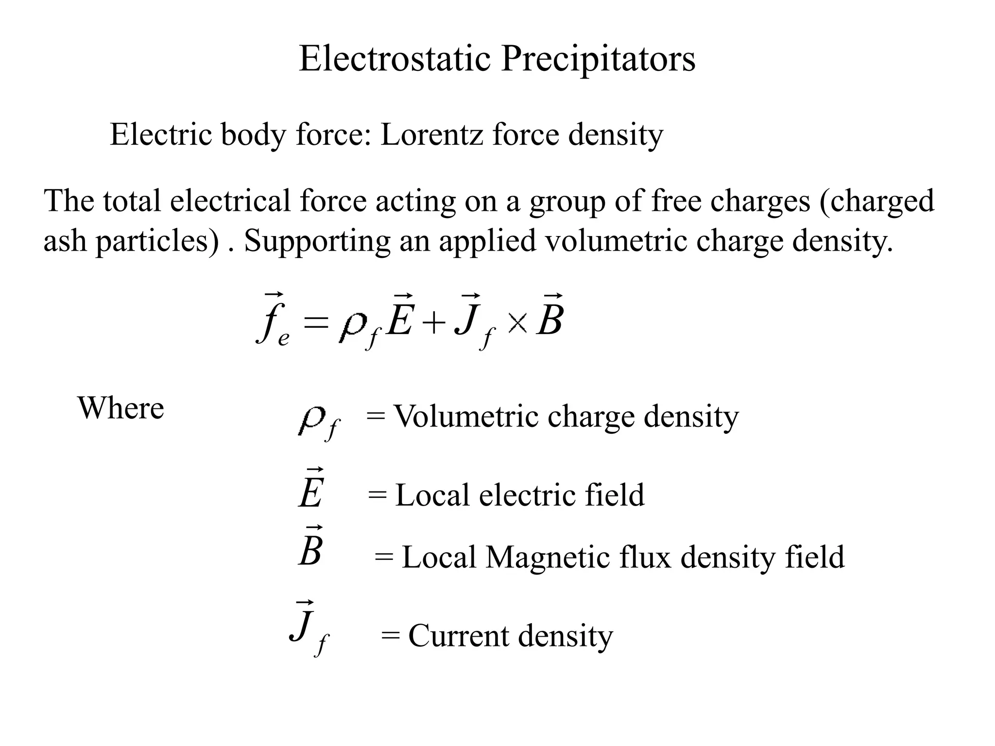
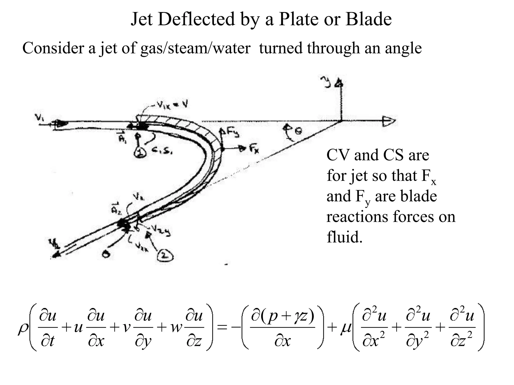
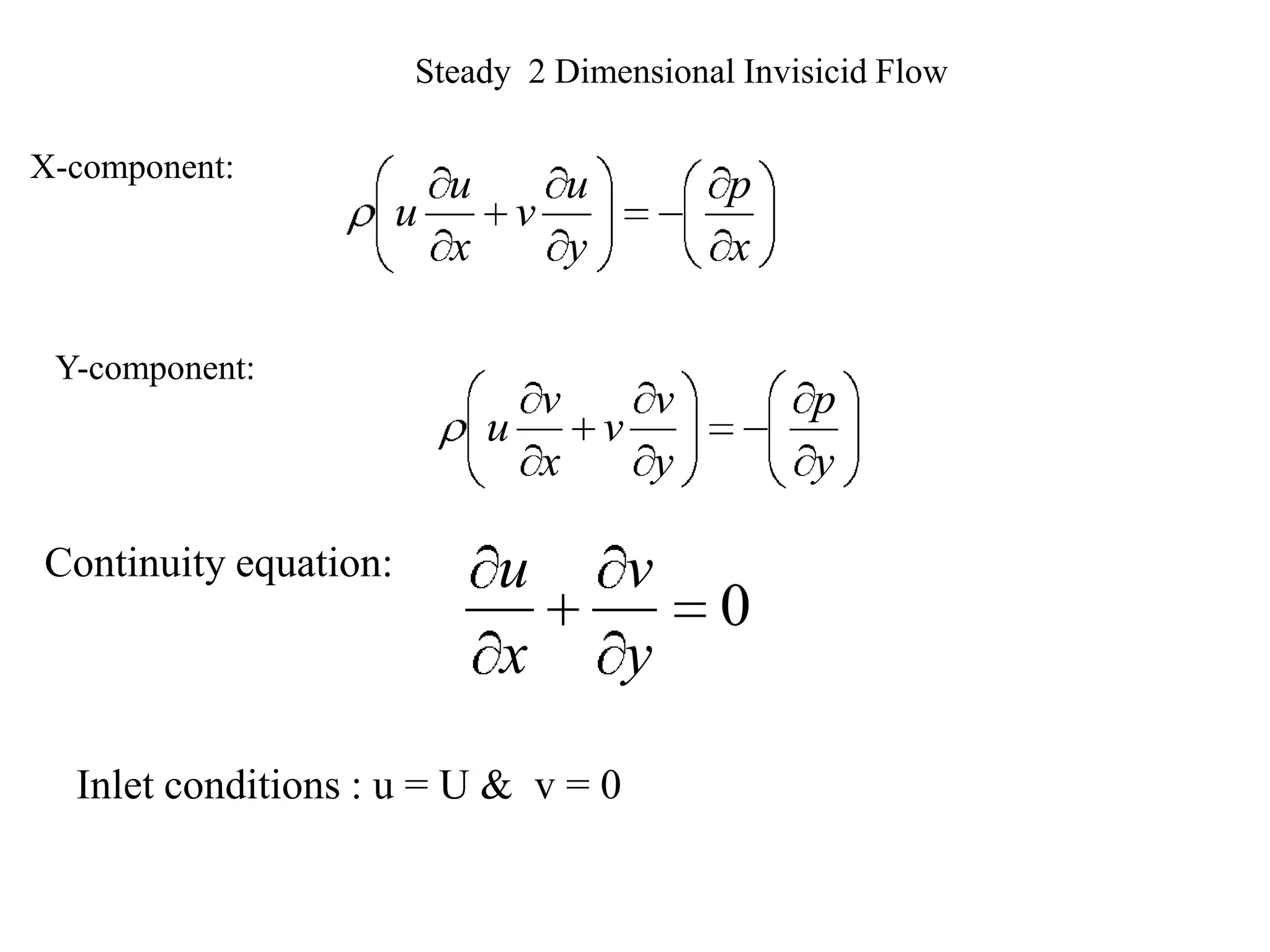
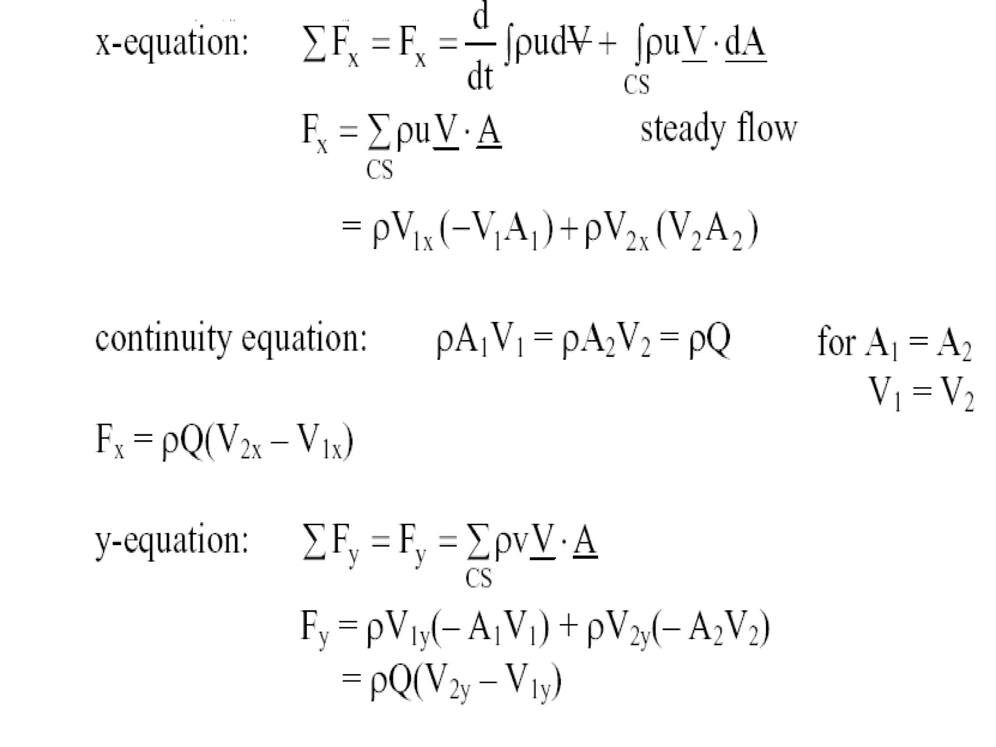
This document provides information about mathematical models for fluid mechanics. It discusses key concepts like streamlines, streamtubes, fluid kinematics, and the conservation laws applied to control volumes using Reynolds Transport Theorem. It also covers fluid properties like pressure variation, ideal fluids, comparison of inertial and viscous forces, and Euler's equation for one-dimensional flow. Important applications of the momentum equation are also highlighted, including jet deflection by a plate and the Navier-Stokes equations in differential form.

1. Mathematical Models for FLUID MECHANICS
P M V Subbarao
Associate Professor
Mechanical Engineering Department
IIT Delhi
Convert Ideas into A Precise Blue Print before
feeling the same....

4. A path line is the trace of the path followed by a selected fluid particle

5. Few things to know about streamlines
• At all points the direction of the streamline is the direction of the
fluid velocity: this is how they are defined.
• Close to the wall the velocity is parallel to the wall so the
streamline is also parallel to the wall.
• It is also important to recognize that the position of streamlines
can change with time - this is the case in unsteady flow.
• In steady flow, the position of streamlines does not change
• Because the fluid is moving in the same direction as the
streamlines, fluid can not cross a streamline.
• Streamlines can not cross each other.
• If they were to cross this would indicate two different velocities at
the same point.
• This is not physically possible.
• The above point implies that any particles of fluid starting on one
streamline will stay on that same streamline throughout the fluid.

6. A useful technique in fluid flow analysis is to consider only a part of the
total fluid in isolation from the rest. This can be done by imagining a
tubular surface formed by streamlines along which the fluid flows. This
tubular surface is known as a streamtube.
A Streamtube
A two dimensional version of the streamtube
The "walls" of a streamtube are made of streamlines.
As we have seen above, fluid cannot flow across a streamline, so
fluid cannot cross a streamtube wall. The streamtube can often be
viewed as a solid walled pipe.
A streamtube is not a pipe - it differs in unsteady flow as the walls
will move with time. And it differs because the "wall" is moving
with the fluid

7. Fluid Kinematics
• The acceleration of a fluid particle is the rate of change of its
velocity.
• In the Lagrangian approach the velocity of a fluid particle is a
function of time only since we have described its motion in terms of
its position vector.

8. In the Eulerian approach the velocity is a function of both
space and time; consequently,

V ˆ j ˆ
u ( x, y, z, t )i v( x, y, z, t ) ˆ w( x, y, z, t )k
   
Velocityco
mponents
x,y,z are f(t) since we must follow the total derivative approach
in evaluating du/dt.

10. Similarly for ay & az,
In vector notation this can be written concisely

13. x
Conservation laws can be applied to an infinitesimal element or
cube, or may be integrated over a large control volume.

14. Basic Control-Volume Approach

15. Control Volume
• In fluid mechanics we are usually interested in a region of space, i.e,
control volume and not particular systems.
• Therefore, we need to transform GDE’s from a system to a control
volume.
• This is accomplished through the use of Reynolds Transport
Theorem.
• Actually derived in thermodynamics for CV forms of continuity and
1st and 2nd laws.

16. Flowing Fluid Through A CV
• A typical control volume for flow
in an funnel-shaped pipe is
bounded by the pipe wall and the
broken lines.
• At time t0, all the fluid (control
mass) is inside the control
volume.

17. The fluid that was in the control volume at time t0 will be seen at
time t0 + t as: .

18. The control volume at time t0 + t .
The control mass at time t0 + t .
The differences between the fluid (control mass) and the control volume
at time t0 + t .

19. • Consider a system and a control volume (C.V.) as follows:
• the system occupies region I and C.V. (region II) at time t0.
• Fluid particles of region – I are trying to enter C.V. (II) at time t0.
III
II
I
• the same system occupies regions (II+III) at t0 + t
• Fluid particles of I will enter CV-II in a time t.
•Few more fluid particles which belong to CV – II at t0 will occupy
III at time t0 + t.

20. The control volume may move as time passes.
III has left CV at time t0+ t
III
II
I is trying to enter CV at time t0
II At time t0+ t

I VCV
At time t0

21. Reynolds' Transport Theorem
• Consider a fluid scalar property b which is the amount of this property
per unit mass of fluid.
• For example, b might be a thermodynamic property, such as the
internal energy unit mass, or the electric charge per unit mass of fluid.
• The laws of physics are expressed as applying to a fixed mass of
material.
• But most of the real devices are control volumes.
• The total amount of the property b inside the material volume M ,
designated by B, may be found by integrating the property per unit
volume, M ,over the material volume :

22. Conservation of B
• total rate of change of any extensive property B of a
system(C.M.) occupying a control volume C.V. at time t is
equal to the sum of
• a) the temporal rate of change of B within the C.V.
• b) the net flux of B through the control surface C.S. that
surrounds the C.V.
• The change of property B of system (C.M.) during Dt is
BCM Bt t
Bt
0 0
BCM BII t0 t
BIII t0 t
BI t0
BII t0
add and subtract B t t
0

23. BCM BII t0 t
BIII t0 t
BI t0
BII t0
BI t0 t
BI t0 t
BCM BI BII t0 t
BIII t0 t
BI BII t0
BI t0 t
BCM BCV t0 t
BCV t0
BIII t0 t
BI t0 t
The above mentioned change has occurred over a time t, therefore
Time averaged change in BCM is
BCM BCV t0 t
BCV t0
BIII t0 t
BI t0 t
t t t t

24. For and infinitesimal time duration
BCM BCV t0 t
BCV t0
BIII t0 t
BI t0 t
lim lim lim lim
t o t t o t t o t t o t
• The rate of change of property B of the system.
dBCM dBCV  
BIII BI
dt dt

25. Conservation of Mass
• Let b=1, the B = mass of the system, m.
dmCM dmCV

mout 
min
dt dt
The rate of change of mass in a control mass should be zero.
dmCV

mout 
min 0
dt

26. Conservation of Momentum
• Let b=V, the B = momentum of the system, mV.
 
d mV d mV  
CM CV

mV out

mV in
dt dt
The rate of change of momentum for a control mass should be equal
to resultant external force.

d mV   
CV

mV out

mV in F
dt

27. Conservation of Energy
• Let b=e, the B = Energy of the system, mV.
d me d me
CM CV

me out

me in
dt dt
The rate of change of energy of a control mass should be equal
to difference of work and heat transfers.
d me  
CV

me out

me in Q W
dt

35. Applications of Momentum Analysis
  

M out 
M in Vn A Vout Vn A Vin F
out in
This is a vector equation and will have three components in x, y and z
Directions.
X – component of momentum equation:
UA U out UA U in Fx
out in

36. X – component of momentum equation:
UA U out UA U in Fx
out in
Y – component of momentum equation:
VA Vout VA Vin Fy
out in
Z – component of momentum equation:
WA Wout WA Win Fz
out in
For a fluid, which is static or moving with uniform velocity, the
Resultant forces in all directions should be individually equal to zero.

37. X – component of momentum equation:
UA U out UA U in Fx
out in
Y – component of momentum equation:
VA Vout VA Vin Fy
out in
Z – component of momentum equation:
WA Wout WA Win Fz
out in
For a fluid, which is static or moving with uniform velocity, the
Resultant forces in all directions should be individually equal to zero.

38. X – component of momentum equation:
Max Fx FB, x FS , x
Y – component of momentum equation:
May Fy FB, y FS , y
Z – component of momentum equation:
Maz Fz FB, z FS , z
For a fluid, which is static or moving with uniform velocity, the
Resultant forces in all directions should be individually equal to zero.

39. Vector equation for momentum:
   
Ma F FB FS
Vector momentum equation per unit volume:
   
a f fB fS

f
Body force per unit volume:B

Gravitational force: f B oi 0 ˆ
ˆ j ˆ
gk

40. Electrostatic Precipitators
Electric body force: Lorentz force density
The total electrical force acting on a group of free charges (charged
ash particles) . Supporting an applied volumetric charge density.
   
fe fE Jf B
Where = Volumetric charge density
f

E = Local electric field
B = Local Magnetic flux density field

Jf = Current density

41. Electric Body Force
• This is also called electrical force density.
• This represents the body force density on a ponderable
medium.
• The Coulomb force on the ions becomes an electrical body
force on gaseous medium.
• This ion-drag effect on the fluid is called as
electrohydrodynamic body force.

42. 0
Ideal Fluids….

43. Pressure Variation in Flowing Fluids
• For fluids in motion, the pressure variation is no longer hydrostatic and is
determined from and is determined from application of Newton’s 2nd Law
to a fluid element.

44. Various Forces in A Flow field
• For fluids in motion, various forces are important:
 
• Inertia Force per unit volume : finertia a

• Body Force: f body ˆ
gk

• Hydrostatic Surface Force: f surface, pressure p
 

• Viscous Surface Force: f surface ,viscous .
• Relative magnitudes of Inertial Forces and Viscous Surface
Force are very important in design of basic fluid devices.

45. Comparison of Magnitudes of Inertia Force and Viscous Force
• Internal vs. External Flows
• Internal flows = completely wall bounded;
• Both viscous and Inertial Forces are important.
• External flows = unbounded; i.e., at some distance from body
or wall flow is uniform.
• External Flow exhibits flow-field regions such that both
inviscid and viscous analysis can be used depending on the
body shape.

46. Ideal or Inviscid Flows
Euler’s Momentum Equation
X – Momentum Equation:

48. Euler’s Equation for One Dimensional Flow
Define an exclusive direction along the
axis of the pipe and corresponding unit
ˆ
direction vector el
Along a path of zero acceleration the
pressure variation is hydrostatic

49. Pressure Variation Due to Acceleration
V V p z
V
t l l
For steady flow along l – direction (stream line)
V P z
V
l l l
Integration of above equation yields

50. Momentum Transfer in A Pump
• Shaft power Disc Power Fluid Power.
2 TN
P Td Td m vdp or m pdv
60
• Flow Machines & Non Flow Machines.
• Compressible fluids & Incompressible Fluids.
• Rotary Machines & Reciprocating Machines.

51. Pump
• Rotate a cylinder containing
fluid at constant speed.
• Supply continuously fluid
from bottom.
• See What happens?
Flow in
•Any More Ideas?

55. Momentum Principle
P M V Subbarao
Associate Professor
Mechanical Engineering Department
IIT Delhi
A primary basis for the design of flow devices ..

56. Momentum Equation

57. Applications of of the Momentum Equation
Initial Setup and Signs
• 1. Jet deflected by a plate or a vane
• 2. Flow through a nozzle
• 3. Forces on bends
• 4. Problems involving non-uniform velocity distribution
• 5. Motion of a rocket
• 6. Force on rectangular sluice gate
• 7. Water hammer

58. Navier-Stokes Equations
Differential form of momentum equation
X-component:
2 2 2
u u u u (p z) u u u
u v w
t x y z x x2 y2 z2
Y-component:
2 2 2
v v v v (p z) v v v
u v w
t x y z y x2 y2 z2

59. z-component:
2 2 2
w w w w (p z) w w w
u v w
t x y z z x2 y2 z2

60. Applications of Momentum Equation

61. Generation of Motive Power Through
Newton’s Second Law

62. Jet Deflected by a Plate or Blade
Consider a jet of gas/steam/water turned through an angle
CV and CS are
for jet so that Fx
and Fy are blade
reactions forces on
fluid.
2 2 2
u u u u (p z) u u u
u v w
t x y z x x2 y2 z2

63. Steady 2 Dimensional Flow
X-component:
2 2
u u (p z) u u
u v
x y x x2 y2
Y-component:
2 2
v v (p z) v v
u v
x y y x2 y2
Continuity equation:
u v u v
0 0
x y x y

64. Steady 2 Dimensional Invisicid Flow
X-component:
u u p
u v
x y x
Y-component:
v v p
u v
x y y
Continuity equation: u v
0
x y
Inlet conditions : u = U & v = 0

65. Pure Impulse Blade
Pressure remains constant along the entire jet.
u u
X-component: u v o
x y
Y-component: v v
u v 0
x y
Continuity equation: u v u v
0
x y x y