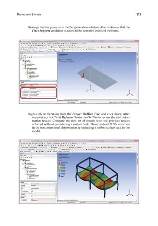
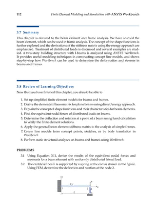
The document describes copyright and trademark information related to ANSYS, Inc. and its software products. It provides legal notices for ANSYS brands, logos, and software names that are trademarks or registered trademarks. It also contains standard copyright information for the book and limitations on copying or redistributing its content.

5. ANSYS, ANSYS Workbench, Ansoft, AUTODYN, CFX, EKM, Engineering Knowledge Manager, FLUENT, HFSS, and
any and all ANSYS, Inc. brand, product, service and feature names, logos and slogans are trademarks or registered trade-
marks of ANSYS, Inc. or its subsidiaries located in the United States or other countries. ICEM CFD is a trademark used
by ANSYS, Inc. under license. CFX is a trademark of Sony Corporation in Japan. All other brand, product, service, and
feature names or trademarks are the property of their respective companies.
CRC Press
Taylor & Francis Group
6000 Broken Sound Parkway NW, Suite 300
Boca Raton, FL 33487-2742
© 2019 by Taylor & Francis Group, LLC
CRC Press is an imprint of Taylor & Francis Group, an Informa business
No claim to original U.S. Government works
Printed on acid-free paper
International Standard Book Number-13: 978-1-1384-8629-4 (Hardback)
This book contains information obtained from authentic and highly regarded sources. Reasonable efforts have been
made to publish reliable data and information, but the author and publisher cannot assume responsibility for the valid-
ity of all materials or the consequences of their use. The authors and publishers have attempted to trace the copyright
holders of all material reproduced in this publication and apologize to copyright holders if permission to publish in this
form has not been obtained. If any copyright material has not been acknowledged please write and let us know so we may
rectify in any future reprint.
Except as permitted under U.S. Copyright Law, no part of this book may be reprinted, reproduced, transmitted, or uti-
lized in any form by any electronic, mechanical, or other means, now known or hereafter invented, including photocopy-
ing, microfilming, and recording, or in any information storage or retrieval system, without written permission from the
publishers.
For permission to photocopy or use material electronically from this work, please access www.copyright.com (http://
www.copyright.com/) or contact the Copyright Clearance Center, Inc. (CCC), 222 Rosewood Drive, Danvers, MA 01923,
978-750-8400. CCC is a not-for-profit organization that provides licenses and registration for a variety of users. For
organizations that have been granted a photocopy license by the CCC, a separate system of payment has been arranged.
Trademark Notice: Product or corporate names may be trademarks or registered trademarks, and are used only for
­
identification and explanation without intent to infringe.
Visit the Taylor & Francis Web site at
http://www.taylorandfrancis.com
and the CRC Press Web site at
http://www.crcpress.com
eResource material is available for this title at https://www.crcpress.com/9781138486294

6. v
Contents
Preface...............................................................................................................................................xi
Authors.......................................................................................................................................... xiii
1. Introduction..............................................................................................................................1
1.1 Some Basic Concepts.....................................................................................................1
1.1.1 Why FEA?..........................................................................................................1
1.1.2 Finite Element Applications in Engineering.................................................1
1.1.3 FEA with ANSYS Workbench...........................................................................3
1.1.4 A Brief History of FEA.....................................................................................3
1.1.5 A General Procedure for FEA.........................................................................4
1.2 An Example in FEA: Spring System............................................................................4
1.2.1 One Spring Element..........................................................................................5
1.2.2 A Spring System................................................................................................6
1.2.2.1 Assembly of Element Equations: Direct Approach......................6
1.2.2.2 Assembly of Element Equations: Energy Approach....................8
1.2.3 Boundary and Load Conditions.....................................................................9
1.2.4 Solution Verification....................................................................................... 10
1.2.5 Example Problems.......................................................................................... 10
1.3 Overview of ANSYS Workbench.................................................................................13
1.3.1 The User Interface...........................................................................................13
1.3.2 The Toolbox...................................................................................................... 14
1.3.3 The Project Schematic.................................................................................... 14
1.3.4 Working with Cells......................................................................................... 16
1.3.5 The Menu Bar.................................................................................................. 16
1.4 Summary.......................................................................................................................17
Problems...................................................................................................................................18
2. Bars and Trusses....................................................................................................................21
2.1 Introduction..................................................................................................................21
2.2 Review of the 1-D Elasticity Theory..........................................................................21
2.3 Modeling of Trusses....................................................................................................22
2.4 Formulation of the Bar Element.................................................................................23
2.4.1 Stiffness Matrix: Direct Method...................................................................23
2.4.2 Stiffness Matrix: Energy Approach..............................................................25
2.4.3 Treatment of Distributed Load.....................................................................27
2.4.4 Bar Element in 2-D and 3-D...........................................................................28
2.4.4.1 2-D Case............................................................................................28
2.4.4.2 3-D Case............................................................................................31
2.4.5 Element Stress.................................................................................................31
2.5 Examples with Bar Elements......................................................................................32
2.6 Case Study with ANSYS Workbench..........................................................................40
2.7 Summary.......................................................................................................................59
2.8 Review of Learning Objectives..................................................................................59
Problems...................................................................................................................................59

7. vi Contents
3. Beams and Frames.................................................................................................................65
3.1 Introduction..................................................................................................................65
3.2 Review of the Beam Theory.......................................................................................65
3.2.1 Euler–Bernoulli Beam and Timoshenko Beam..........................................65
3.2.2 Stress, Strain, Deflection, and Their Relations...........................................67
3.3 Modeling of Beams and Frames................................................................................68
3.3.1 Cross Sections and Strong/Weak Axis........................................................68
3.3.2 Support Conditions........................................................................................69
3.3.3 Conversion of a Physical Model into a Line Model...................................70
3.4 Formulation of the Beam Element.............................................................................70
3.4.1 Element Stiffness Equation: The Direct Approach....................................71
3.4.2 Element Stiffness Equation: The Energy Approach..................................72
3.4.3 Treatment of Distributed Loads.................................................................... 74
3.4.4 Stiffness Matrix for a General Beam Element.............................................75
3.5 Examples with Beam Elements.................................................................................. 76
3.6 Case Study with ANSYS Workbench..........................................................................85
3.7 Summary..................................................................................................................... 112
3.8 Review of Learning Objectives................................................................................ 112
Problems................................................................................................................................. 112
4. Two-Dimensional Elasticity.............................................................................................. 117
4.1 Introduction................................................................................................................ 117
4.2 Review of 2-D Elasticity Theory.............................................................................. 117
4.2.1 Plane Stress.................................................................................................... 117
4.2.2 Plane Strain.................................................................................................... 118
4.2.3 Stress–Strain (Constitutive) Equations...................................................... 119
4.2.4 Strain and Displacement Relations............................................................120
4.2.5 Equilibrium Equations................................................................................. 121
4.2.6 Boundary Conditions................................................................................... 121
4.2.7 Exact Elasticity Solution............................................................................... 121
4.3 Modeling of 2-D Elasticity Problems.......................................................................122
4.4 Formulation of the Plane Stress/Strain Element...................................................123
4.4.1 A General Formula for the Stiffness Matrix............................................. 124
4.4.2 Constant Strain Triangle (CST or T3)......................................................... 124
4.4.3 Quadratic Triangular Element (LST or T6)...............................................129
4.4.4 Linear Quadrilateral Element (Q4).............................................................130
4.4.5 Quadratic Quadrilateral Element (Q8)....................................................... 131
4.4.6 Transformation of Loads.............................................................................. 132
4.4.7 Stress Calculation.........................................................................................134
4.4.7.1 The von Mises Stress....................................................................134
4.4.7.2 Averaged Stresses..........................................................................135
4.4.8 General Comments on the 2-D Elements..................................................136
4.5 Case Study with ANSYS Workbench........................................................................ 137
4.6 Summary.....................................................................................................................155
4.7 Review of Learning Objectives................................................................................155
Problems.................................................................................................................................156
5. Modeling and Solution Techniques................................................................................ 161
5.1 Introduction................................................................................................................ 161

8. vii
Contents
5.2 Symmetry.................................................................................................................... 161
5.2.1 An Example................................................................................................... 162
5.3 Substructures (Superelements)................................................................................ 163
5.4 Equation Solving........................................................................................................164
5.4.1 Direct Methods (Gauss Elimination).........................................................164
5.4.2 Iterative Methods..........................................................................................164
5.4.3 An Example: Gauss Elimination.................................................................164
5.4.4 An Example: Iterative Method.................................................................... 165
5.5 Nature of Finite Element Solutions......................................................................... 166
5.6 Convergence of FEA Solutions................................................................................. 167
5.7 Adaptivity (h-, p-, and hp-Methods)......................................................................... 167
5.8 Case Study with ANSYS Workbench........................................................................ 168
5.9 Summary..................................................................................................................... 182
5.10 Review of Learning Objectives................................................................................183
Problems.................................................................................................................................183
6. Plate and Shell Analyses.................................................................................................... 187
6.1 Introduction................................................................................................................ 187
6.2 Review of Plate Theory............................................................................................. 187
6.2.1 Force and Stress Relations in Plates........................................................... 187
6.2.2 Thin Plate Theory (Kirchhoff Plate Theory)............................................. 189
6.2.2.1 Example: A Thin Plate.................................................................. 191
6.2.3 Thick Plate Theory (Mindlin Plate Theory).............................................. 192
6.2.4 Shell Theory................................................................................................... 193
6.2.4.1 Shell Example: A Cylindrical Container.................................... 193
6.3 Modeling of Plates and Shells.................................................................................. 194
6.4 Formulation of the Plate and Shell Elements......................................................... 195
6.4.1 Kirchhoff Plate Elements............................................................................. 195
6.4.2 Mindlin Plate Elements................................................................................ 196
6.4.3 Discrete Kirchhoff Elements....................................................................... 197
6.4.4 Flat Shell Elements........................................................................................ 197
6.4.5 Curved Shell Elements................................................................................. 198
6.5 Case Studies with ANSYS Workbench......................................................................199
6.6 Summary..................................................................................................................... 214
6.7 Review of Learning Objectives................................................................................ 214
Problems................................................................................................................................. 214
7. Three-Dimensional Elasticity........................................................................................... 219
7.1 Introduction................................................................................................................ 219
7.2 Review of Theory of Elasticity................................................................................. 219
7.2.1 Stress–Strain Relation..................................................................................220
7.2.2 Displacement.................................................................................................221
7.2.3 Strain–Displacement Relation.....................................................................221
7.2.4 Equilibrium Equations.................................................................................221
7.2.5 Boundary Conditions...................................................................................222
7.2.6 Stress Analysis..............................................................................................222
7.3 Modeling of 3-D Elastic Structures.........................................................................222
7.3.1 Mesh Discretization......................................................................................223
7.3.2 Boundary Conditions: Supports.................................................................223

9. viii Contents
7.3.3 Boundary Conditions: Loads......................................................................224
7.3.4 Assembly Analysis: Contacts......................................................................224
7.4 Formulation of Solid Elements.................................................................................225
7.4.1 General Formulation....................................................................................225
7.4.2 Typical Solid Element Types.......................................................................226
7.4.3 Formulation of a Linear Hexahedral Element Type................................227
7.4.4 Treatment of Distributed Loads..................................................................230
7.5 Case Studies with ANSYS Workbench......................................................................230
7.6 Summary.....................................................................................................................255
7.7 Review of Learning Objectives................................................................................255
Problems.................................................................................................................................255
8. Structural Vibration and Dynamics................................................................................ 261
8.1 Introduction................................................................................................................ 261
8.2 Review of Basic Equations........................................................................................ 261
8.2.1 A Single DOF System...................................................................................262
8.2.2 A Multi-DOF System....................................................................................264
8.2.2.1 Mass Matrices................................................................................264
8.2.2.2 Damping.........................................................................................266
8.3 Formulation for Modal Analysis............................................................................. 267
8.3.1 Modal Equations...........................................................................................269
8.4 Formulation for Frequency Response Analysis....................................................271
8.4.1 Modal Method...............................................................................................271
8.4.2 Direct Method...............................................................................................272
8.5 Formulation for Transient Response Analysis......................................................272
8.5.1 Direct Methods (Direct Integration Methods)..........................................273
8.5.2 Modal Method............................................................................................... 274
8.6 Modeling Examples...................................................................................................275
8.6.1 Modal Analysis.............................................................................................275
8.6.2 Frequency Response Analysis.................................................................... 276
8.6.3 Transient Response Analysis...................................................................... 276
8.6.4 Cautions in Dynamic Analysis................................................................... 276
8.7 Case Studies with ANSYS Workbench......................................................................277
8.8 Summary.....................................................................................................................293
8.9 Review of Learning Objectives................................................................................294
Problems.................................................................................................................................294
9. Thermal Analysis................................................................................................................301
9.1 Introduction................................................................................................................301
9.2 Review of Basic Equations........................................................................................301
9.2.1 Thermal Analysis..........................................................................................301
9.2.1.1 Finite Element Formulation for Heat Conduction....................303
9.2.2 Thermal Stress Analysis..............................................................................303
9.2.2.1 1-D Case..........................................................................................304
9.2.2.2 2-D Cases........................................................................................305
9.2.2.3 3-D Case..........................................................................................305
9.2.2.4 Notes on FEA for Thermal Stress Analysis...............................305
9.3 Modeling of Thermal Problems...............................................................................306
9.3.1 Thermal Analysis..........................................................................................306

10. ix
Contents
9.3.2 Thermal Stress Analysis..............................................................................306
9.4 Case Studies with ANSYS Workbench......................................................................308
9.5 Summary.....................................................................................................................330
9.6 Review of Learning Objectives................................................................................330
Problems.................................................................................................................................330
10. Introduction to Fluid Analysis.........................................................................................337
10.1 Introduction................................................................................................................337
10.2 Review of Basic Equations........................................................................................337
10.2.1 Describing Fluid Motion..............................................................................337
10.2.2 Types of Fluid Flow......................................................................................337
10.2.3 Navier–Stokes Equations.............................................................................338
10.3 Modeling of Fluid Flow.............................................................................................339
10.3.1 Fluid Domain................................................................................................339
10.3.2 Meshing..........................................................................................................339
10.3.3 Boundary Conditions...................................................................................339
10.3.4 Solution Visualization..................................................................................340
10.4 Case Studies with ANSYS Workbench......................................................................341
10.5 Summary.....................................................................................................................368
10.6 Review of Learning Objectives................................................................................368
Problems.................................................................................................................................368
11. Design Optimization..........................................................................................................373
11.1 Introduction................................................................................................................373
11.2 Topology Optimization.............................................................................................373
11.3 Parametric Optimization.......................................................................................... 374
11.4 Design Space Exploration for Parametric Optimization...................................... 374
11.4.1 Design of Experiments.................................................................................375
11.4.2 Response Surface Optimization.................................................................377
11.5 Case Studies with ANSYS Workbench......................................................................377
11.6 Summary..................................................................................................................... 415
11.7 Review of Learning Objectives................................................................................ 415
Problems................................................................................................................................. 415
12. Failure Analysis................................................................................................................... 419
12.1 Introduction................................................................................................................ 419
12.2 Static Failure............................................................................................................... 419
12.2.1 Ductile Failure............................................................................................... 419
12.2.1.1 Maximum Shear Stress Theory (Tresca Criterion)................... 419
12.2.1.2 Distortion Energy Theory (von Mises Criterion)......................420
12.2.2 Brittle Failure.................................................................................................420
12.2.2.1 Maximum Normal Stress Theory...............................................420
12.2.2.2 Mohr–Coulomb Theory...............................................................420
12.3 Fatigue Failure............................................................................................................421
12.3.1 Soderberg Failure Criterion.........................................................................422
12.3.2 Goodman Failure Criterion.........................................................................422
12.3.3 Gerber Failure Criterion...............................................................................423
12.4 Buckling Failure.........................................................................................................424
12.5 Case Studies with ANSYS Workbench......................................................................425

11. x Contents
12.6 Summary.....................................................................................................................436
12.7 Review of Learning Objectives................................................................................436
Problems.................................................................................................................................437
Appendix 1: Review of Matrix Algebra.................................................................................441
Appendix 2: Photo Credits........................................................................................................447
References....................................................................................................................................449
Index..............................................................................................................................................451

12. xi
Preface
This book presents an integrated introduction to the basic theories of finite element
analysis (FEA) and the use of ANSYS® Workbench in the modeling and simulation of
engineering problems. It is intended for undergraduate students in engineering and
for engineers who have no previous experience with the FEA and wish to learn the
basic theory and software usage from a single volume. The book covers the basic con-
cepts in the FEA using simple mechanics problems as examples, and leads to discus-
sions and applications of the one-dimensional bar and beam elements, two-dimensional
plane stress and plane strain elements, plate and shell elements, and three-dimensional
solid elements in the analyses of structural stresses, vibrations and dynamics, thermal
responses, fluid flows, optimizations, and failures. In each of these application areas,
ANSYS Workbench is introduced through hands-on case studies. Clear understanding of
the FEA principles, element behaviors, solution procedures, and correct usage of the FEA
software is emphasized throughout the book.
The materials in this book are good for teaching undergraduate FEA courses in engineer-
ing to students who need a general background in the FEA so that they can apply FEA in
their design and analysis of structures using ANSYS Workbench or other FEA software.
Presentations of FEA theories and formulations in the book are kept to a minimum, aimed
solely for readers to understand the behaviors of the various elements and FEA solutions.
Emphases are placed on the techniques in FEA modeling and simulation, such as in build-
ing a quality FEA mesh, verifying the results, and employing the symmetry of a struc-
ture. The book includes 12 chapters and can be used for an undergraduate FEA course in
one semester (15 weeks with three 50-minute sessions each week) or in two quarters (10
weeks per quarter with three 50-minute sessions each week). It is recommended that com-
puter lab sessions on using ANSYS Workbench be arranged for each chapter. Case studies
included in the book provide step-by-step instructions on solving a variety of problems of
moderate size and level of sophistication in ANSYS Workbench, and can be covered in the
lab sessions. Modeling tips are available in the case studies wherever applicable to give
students an immediate opportunity to use the skills they learn in a problem-solving con-
text. Homework problems and projects using ANSYS Workbench software are provided at
the end of each chapter.
The Solutions Manual contains solutions to all end-of-chapter problems. The manual
features a compact presentation of solutions for over 100 problems. Each end-of-chapter
problem that requires the use of an FEA tool is solved in ANSYS Workbench. For such a prob-
lem, the Workbench solution, which contains crucial properties such as geometry, material,
mesh, boundary conditions, and simulation results, is saved using a Workbench project file
(.wbpj) as well as a project folder that contains the supporting files for the Workbench project.
The Solutions Manual, along with the Workbench solution files for over 80 end-of-chapter
simulationproblems,isavailabletoinstructorsfromCRCPress.MicrosoftPowerPointslides
for each chapter are provided to instructors using this book. In addition, Workbench files
for the case studies are available to instructors for use in lectures or computer lab ­
sessions.
The additional material is available from the CRC website: https:/
/www.crcpress.com/
Finite-Element-Modeling-and-Simulation-with-ANSYS-Workbench-Second-Edition/
Chen-Liu/p/book/9781138486294

13. xii Preface
The materials in the book have been developed by the authors for undergraduate
courses on FEA at the Washington State University Vancouver and at the University
of Cincinnati for the last 10 years or so. The authors would like to thank many of their
­
current and former students for their help in developing these lecture materials and
their contributions to many of the examples used in the book, and in particular we thank
students Qikai Xie, Fan Yang, and Bin He for their help in developing the supplementary
materials for this book. We are grateful for the students we met in our classes at Vancouver
and Cincinnati. This book could never have been written without their collective inter-
est, feedback, and enthusiasm. Our special thanks go to the editorial staff at CRC Press,
Jonathan Plant, the Senior Editor, and Amber Donley, the Project Coordinator, for their
patience, cooperation, and professionalism in the production of this book. Much grati-
tude also goes to the reviewers for their valuable comments and suggestions. Of course,
we take full responsibility for any errors or mistakes in the book. We also ­
welcome any
suggestions from readers that could help us improve the book in the future.
Xiaolin Chen
Vancouver, Washington
Yijun Liu
Cincinnati, Ohio

14. xiii
Authors
Dr. Xiaolin Chen is an associate professor of mechanical engineering at the Washington
State University Vancouver. She earned her BS in engineering mechanics from Shanghai
Jiao Tong University, MS in mechanical design and theory from the State Key Laboratory
of Mechanical System and Vibration affiliated with Shanghai Jiao Tong University, and
her PhD in mechanical engineering from the University of Cincinnati. Her research inter-
ests include computational mechanics, finite element analysis, boundary element analysis,
multiphysics phenomena and coupled-field problems, inverse problems, and model order
reduction techniques.
Dr. Yijun Liu is a professor of mechanical engineering at the University of Cincinnati.
He earned his BS and MS in aerospace engineering from Northwestern Polytechnical
University (China), and his PhD in theoretical and applied mechanics from the University
of Illinois at Urbana-Champaign. Prior to joining the faculty, he conducted postdoctoral
research at the Center of Nondestructive Evaluation of Iowa State University and worked
at Ford Motor Company as a CAE analyst. Dr. Liu’s interests are in computational mechan-
ics, finite element method, boundary element method, and fast multipole method in mod-
eling composite materials, fracture, fatigue, structural dynamics, and acoustics problems.
He is the author of the book Fast Multipole Boundary Element Method (Cambridge University
Press, 2009) and has had more than 100 papers published in technical journals and confer-
ence proceedings in areas of computational mechanics.

16. 1
1
Introduction
1.1 Some Basic Concepts
The finite element method (FEM), or finite element analysis (FEA), is based on the idea of
building a complicated object with simple blocks, or, dividing a complicated object into
smaller and manageable pieces. Application of this simple idea can be found everywhere
in everyday life (Figure 1.1), as well as in engineering. For example, children play with
LEGO® toys by using many small pieces, each of very simple geometry, to build vari-
ous objects such as trains, ships, or buildings. With more and more smaller pieces, these
objects will look more realistic.
In mathematical terms, this is simply the use of the limit concept, that is, to approach or
represent a smooth object with a finite number of simple pieces and increasing the number
of such pieces in order to improve the accuracy of this representation.
1.1.1 Why FEA?
Computers have revolutionized the practice of engineering. Design of a product that used
to be done by tedious hand drawings has been replaced by computer-aided design (CAD)
using computer graphics. Analysis of a design used to be done by hand calculations and
many of the testing have been replaced by computer simulations using computer-aided
engineering (CAE) software. Together, CAD, CAE, and computer-aided manufacturing
(CAM) have dramatically changed the landscape of engineering (Figure 1.2). For example,
a car, that used to take five to six years from design to product, can now be produced start-
ing from the concept design to the manufacturing within a year using the CAD/CAE/
CAM technologies.
Among all the computational tools for CAE, the FEM is the most widely applied method
or one of the most powerful modern “calculators” available for engineering students and
professionals. FEA provides a way of virtually testing a product design. It helps users
understand their designs and implement appropriate design changes early in the product
development process. The adoption of FEA in the design cycle is driven by market pres-
sure since it brings many benefits that will help companies make better products with
reduced development costs and time-to-market.
1.1.2 Finite Element Applications in Engineering
The FEM can be applied in solving the mathematical models of many engineering prob-
lems, from stress analysis of truss and frame structures or complicated machines, to
dynamic responses of automobiles, trains, or airplanes under different mechanical,

17. 2 Finite Element Modeling and Simulation with ANSYS Workbench
thermal, or electromagnetic loading. There are numerous finite element applications
in industries, ranging from automotive, aerospace, defense, consumer products, and
industrial equipment to energy, transportation and construction, as shown by some
examples in Table 1.1. The applications of the FEA have also been extended to materials
science, biomedical engineering, geophysics, and many other emerging fields in recent
years.
CAD
Design
concept
Design
modeling
Design
optimization
Design
evaluation
Production
planning
Process
planning
Quality
control
Packaging
Customer
market
Design
analysis
CAE
CAM
FIGURE 1.2
A sketch of the computer-aided product development process.
FIGURE 1.1
Objects built with simple and small pieces: (a) a fire engine built with LEGO® (http://lego.wikia.com/
wiki/10020_Santa_Fe_Super_Chief); and (b) a house built with many elements—bricks, beams, columns, pan-
els, and so on.
TABLE 1.1
Examples of Engineering Applications Using FEA
Field of Study Examples of Engineering Applications
Structural and solid mechanics Offshore structure reliability analysis, vehicle crash simulation,
nuclear reactor component integrity analysis, wind turbine blade
design optimization
Heat transfer Electronics cooling modeling, casting modeling, combustion engine
heat-transfer analysis
Fluid flow Aerodynamic analysis of race car designs, modeling of airflow
patterns in buildings, seepage analysis through porous media
Electrostatics/electromagnetics Field calculations in sensors and actuators, performance prediction of
antenna designs, electromagnetic interference suppression analysis

18. 3
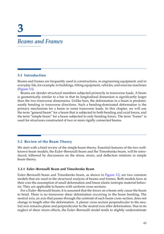
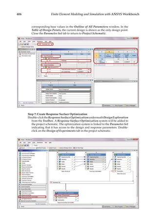
Introduction
1.1.3 FEA with ANSYS Workbench
Over the last few decades, many commercial programs have become available for con-
ducting the FEA. Among a comprehensive range of finite element simulation solutions
­
provided by leading CAE companies, ANSYS® Workbench is a user-friendly platform
designed to seamlessly integrate ANSYS, Inc.’s suite of advanced engineering simulation
technology. It offers bidirectional connection to major CAD systems. The Workbench envi-
ronment is geared toward improving productivity and ease of use among engineering
teams. It has evolved as an indispensible tool for product development at a growing num-
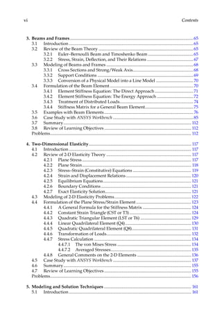
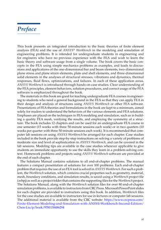
ber of companies, finding applications in many diverse engineering fields (Figure 1.3).
1.1.4 A Brief History of FEA
An account of the historical development of FEM and the computational mechanics in
general was given by O. C. Zienkiewicz recently, which can be found in Reference [1]. The
foundation of the FEM was first developed by Courant in the early 1940s. The stiffness
method, a prelude of the FEM, was developed by Turner, Clough et al., in 1956. The name
“finite element” was coined by Clough in 1960. Computer implementation of FEM pro-
grams emerged during the early 1970s. To date, FEM has become one of the most widely
used and versatile analysis techniques. A few major milestones are as follows:
1943—Courant (Variational methods which laid the foundation for FEM)
1956—Turner, Clough, Martin, and Topp (Stiffness method)
1960—Clough (Coined “Finite Element,” solved plane problems)
1970s—Applications on “mainframe” computers
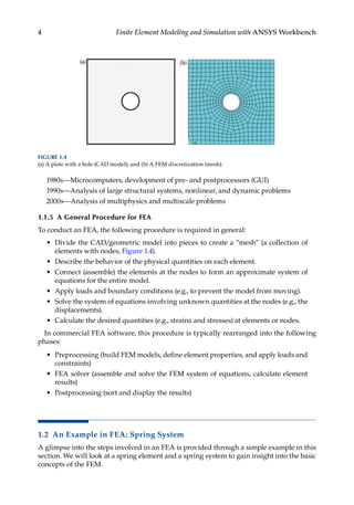
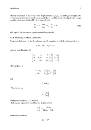
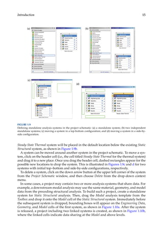
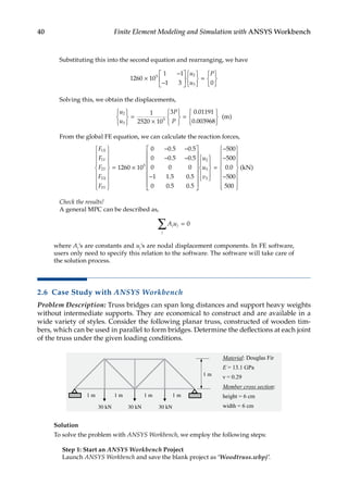
FIGURE 1.3
Examples of FEA using ANSYS Workbench: (a) wind load simulation of an offshore platform (Courtesy of
ANSYS, Inc., http://www.ansys.com/Industries/Energy/Oil+&+Gas); (b) modal response of a steel frame
building with concrete slab floors (http://www.isvr.co.uk/modelling/); (c) underhood flow and thermal man-
agement (Courtesy of ANSYS, Inc., http://www.ansys.com/Industries/Automotive/Application+Highlights/
Underhood); and (d) electric field pattern of antenna mounted on helicopter (Courtesy of ANSYS, Inc., http://
www.ansys.com/Industries/Electronics+&+Semiconductor/Defense+&+Aerospace + Electronics).

19. 4 Finite Element Modeling and Simulation with ANSYS Workbench
1980s—Microcomputers, development of pre- and postprocessors (GUI)
1990s—Analysis of large structural systems, nonlinear, and dynamic problems
2000s—Analysis of multiphysics and multiscale problems
1.1.5 A General Procedure for FEA
To conduct an FEA, the following procedure is required in general:
• Divide the CAD/geometric model into pieces to create a “mesh” (a collection of
elements with nodes, Figure 1.4).
• Describe the behavior of the physical quantities on each element.
• Connect (assemble) the elements at the nodes to form an approximate system of
equations for the entire model.
• Apply loads and boundary conditions (e.g., to prevent the model from moving).
• Solve the system of equations involving unknown quantities at the nodes (e.g., the
displacements).
• Calculate the desired quantities (e.g., strains and stresses) at elements or nodes.
In commercial FEA software, this procedure is typically rearranged into the following
phases:
• Preprocessing (build FEM models, define element properties, and apply loads and
constraints)
• FEA solver (assemble and solve the FEM system of equations, calculate element
results)
• Postprocessing (sort and display the results)
1.2 An Example in FEA: Spring System
A glimpse into the steps involved in an FEA is provided through a simple example in this
section. We will look at a spring element and a spring system to gain insight into the basic
concepts of the FEM.
FIGURE 1.4
(a) A plate with a hole (CAD model); and (b) A FEM discretization (mesh).

20. 5
Introduction
1.2.1 One Spring Element
For the single element shown in Figure 1.5, we have:
Two nodes i, j
Nodal displacements ui, uj (m, mm)
Nodal forces fi, fj (Newton)
Spring constant (stiffness) k (N/m, N/mm)
Relationship between spring force F and elongation Δ is shown in Figure 1.6.
In the linear portion of the curve shown in Figure 1.6, we have
F = kΔ, with Δ = uj − ui (1.1)
where k = F/Δ(>0) is the stiffness of the spring (the force needed to produce a unit stretch).
Consider the equilibrium of forces for the spring. At node i, we have
fi = −F = −k(uj − ui) = kui − kuj
fi i F
and at node j
fj = F = k(uj − ui) = −kui + kuj
F j fj
In matrix form,
k k
k k
u
u
f
f
i
j
i
j
−
−













=







(1.2)
F
Nonlinear
∆
Linear
k
FIGURE 1.6
Force–displacement relation in a spring.
k
i j
uj
ui
fi fj
x
FIGURE 1.5
One spring element.

21. 6 Finite Element Modeling and Simulation with ANSYS Workbench
or,
ku = f (1.3)
where
k = element stiffness matrix
u = element nodal displacement vector
f = element nodal force vector
From the derivation, we see that the first equation in Equation 1.2 represents the equilib-
rium of forces at node i, while the second equation in Equation 1.2 represents the equilib-
rium of forces at node j. Note also that k is symmetric. Is k singular or nonsingular? That
is, can we solve the equation in Equation 1.2? If not, why?
1.2.2 A Spring System
For a system of multiple spring elements, we first write down the stiffness equation for
each spring and then “assemble” them together to form the stiffness equation for the whole
system. For example, for the two-spring system shown in Figure 1.7, we proceed as follows:
For element 1, we have
k k
k k
u
u
f
f
1 1
1 1
1
2
1
1
2
1
−
−












=










(1.4)
and for element 2,
k k
k k
u
u
f
f
2 2
2 2
2
3
1
2
2
2
−
−












=










(1.5)
where fi
m
is the (internal) force acting on local node i of element m (i = 1, 2).
1.2.2.1 Assembly of Element Equations: Direct Approach
Consider the equilibrium of forces at node 1,
F f
1 1
1
=
F1
1 f1
1
k1
u1, F1
x
k2
u2, F2 u3, F3
1 2 3
FIGURE 1.7
A system of two spring elements.

22. 7
Introduction
at node 2,
f2
1 2 f1
2
F2
F f f
2 2
1
1
2
= +
and, at node 3,
F f
3 2
2
=
f2
2
3 F3
Using Equations 1.4 and 1.5, we obtain
F k u k u
F k u k k u k u
F k u k u
1 1 1 1 2
2 1 1 1 2 2 2 3
3 2 2 2 3
= −
= − + + −
= − +
( )
In matrix form, we have
k k
k k k k
k k
u
u
u
F
F
F
1 1
1 1 2 2
2 2
1
2
3
1
2
3
0
0
−
− + −
−




















=











(1.6)
or
Ku = F (1.7)
in which, K is the stiffness matrix (structure matrix) for the entire spring system.
1.2.2.1.1 An Alternative Way of Assembling the Whole Stiffness Matrix
“Enlarging” the stiffness matrices for elements 1 and 2, we have
k k
k k
u
u
u
f
f
1 1
1 1
1
2
3
1
1
2
1
0
0
0 0 0 0
−
−




















=











and
0 0 0
0
0
0
2 2
2 2
1
2
3
1
2
2
2
k k
k k
u
u
u
f
f
−
−




















=












23. 8 Finite Element Modeling and Simulation with ANSYS Workbench
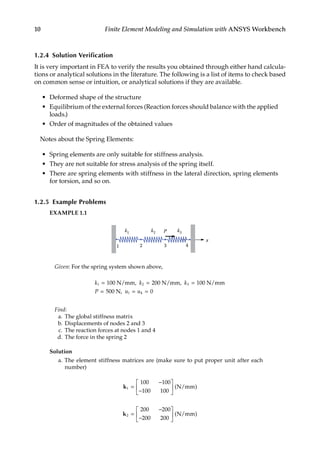
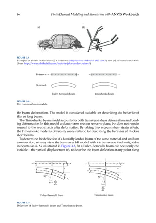
Adding the two matrix equations (i.e., using superposition), we have
k k
k k k k
k k
u
u
u
f
f f
1 1
1 1 2 2
2 2
1
2
3
1
1
2
1
0
0
−
− + −
−




















= + 1
1
2
2
2
f










This is the same equation we derived by using the concept of equilibrium of forces.
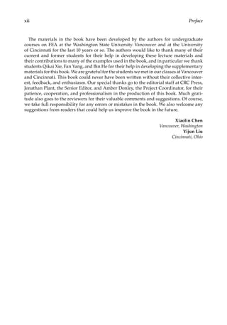
1.2.2.2 Assembly of Element Equations: Energy Approach
We can also obtain the result using an energy method, for example, the principle of mini-
mum potential energy. In fact, the energy approach is more general and considered the
foundation of the FEM. To proceed, we consider the strain energy U stored in the spring
system shown in Figure 1.5.
U = + = +
1
2
1
2
1
2
1
2
1 1
2
2 2
2
1 1 1 2 2 2
k k k k
T T
∆ ∆ ∆ ∆ ∆ ∆
However,
∆ ∆
1 2 1
1
2
2 3 2
2
3
1 1 1 1
= − = −






= − = −






u u
u
u
u u
u
u
[ ] , [ ]
We have
U =
−
−












+
−
−



1
2
1
2
1 2
1 1
1 1
1
2
2 3
2 2
2 2
[ ] [ ]
u u
k k
k k
u
u
u u
k k
k k










=
−
− + −
−
= …
u
u
u u u
k k
k k k k
k
2
3
1 2 3
1 1
1 1 2 2
1
2
0
0
( )
[ ]
enlarging
2
2 2
1
2
3
k
u
u
u




















(1.8)
The potential of the external forces is
Ω = − − − = −










F u F u F u u u u
F
F
F
1 1 2 2 3 3 1 2 3
1
2
3
[ ] (1.9)
Thus, the total potential energy of the system is
Π Ω
= + =
−
− + −
−













U
1
2
0
0
1 2 3
1 1
1 1 2 2
2 2
1
2
3
[ ]
u u u
k k
k k k k
k k
u
u
u








−










[ ]
u u u
F
F
F
1 2 3
1
2
3
(1.10)

24. 9
Introduction
which is a function of the three nodal displacements (u1,u2,u3). According to the principle
of minimum potential energy, for a system to be in equilibrium, the total potential energy
must be minimum, that is, dΠ = 0, or equivalently,
∂
∂
∂
∂
∂
∂
Π Π Π
u u u
1 2 3
0 0 0
= = =
, , , (1.11)
which yield the same three equations as in Equation 1.6.
1.2.3 Boundary and Load Conditions
Assuming that node 1 is fixed, and same force P is applied at node 2 and node 3, that is
u1 = 0 and F2 = F3 = P
we have from Equation 1.6
k k
k k k k
k k
u
u
F
P
P
1 1
1 1 2 2
2 2
2
3
1
0
0
0
−
− + −
−




















=











which reduces to
k k k
k k
u
u
P
P
1 2 2
2 2
2
3
+ −
−












=






and
F1 = −k1u2
Unknowns are
u =






u
u
2
3
and the reaction force F1 (if desired).
Solving the equations, we obtain the displacements
u
u
P k
P k P k
2
3
1
1 2
2
2






=
+






/
/ /
and the reaction force
F1 = −2P

25. 10 Finite Element Modeling and Simulation with ANSYS Workbench
1.2.4 Solution Verification
It is very important in FEA to verify the results you obtained through either hand calcula-
tions or analytical solutions in the literature. The following is a list of items to check based
on common sense or intuition, or analytical solutions if they are available.
• Deformed shape of the structure
• Equilibrium of the external forces (Reaction forces should balance with the applied
loads.)
• Order of magnitudes of the obtained values
Notes about the Spring Elements:
• Spring elements are only suitable for stiffness analysis.
• They are not suitable for stress analysis of the spring itself.
• There are spring elements with stiffness in the lateral direction, spring elements
for torsion, and so on.
1.2.5 Example Problems
EXAMPLE 1.1
k1
x
k2
1 2 3
k3
4
P
Given: For the spring system shown above,
k k k
P u u
1 2 3
4 0
= = =
= = =
100 N/mm, 200 N/mm, 100 N/mm
500 N, 1
Find:
a. The global stiffness matrix
b. Displacements of nodes 2 and 3
c. The reaction forces at nodes 1 and 4
d. The force in the spring 2
Solution
a. The element stiffness matrices are (make sure to put proper unit after each
number)
k1
100 100
100 100
=
−
−





 ( )
N/mm
k2
200 200
200 200
=
−
−





 ( )
N/mm

26. 11
Introduction
k3
100 100
100 100
=
−
−





 ( )
N/mm
Applying the superposition concept, we obtain the global stiffness matrix
for the spring system
u u u u
1 2 3 4
100 100 0 0
100 100 200 200 0
0 200 200 100 100
0 0 100 1
K =
−
− + −
− + −
− 0
00














or
K =
−
− −
− −
−














100 100 0 0
100 300 200 0
0 200 300 100
0 0 100 100
which is symmetric and banded.
Equilibrium (FE) equation for the whole system is
100 100 0 0
100 300 200 0
0 200 300 100
0 0 100 100
1
−
− −
− −
−














u
u
u
u
u
F
F
F
F
2
3
4
1
2
3
4














=














b. Applying the BCs u1 = u4 = 0, F2 = 0, and F3 = P, and “deleting” the first and
fourth rows and columns, we have
300 200
200 300
0
2
3
−
−













=







u
u P
Solving this equation, we obtain
u
u
P
P
2
3
250
3 500
2
3







=







=







/
/
(mm)
c. From the first and fourth equations in the system of FE equations, we obtain
the reaction forces
F u
1 2
100 200
= − = − ( )
N
F u
4 3
100 300
= − = − ( )
N

27. 12 Finite Element Modeling and Simulation with ANSYS Workbench
d. The FE equation for spring (element) 2 is
200 200
200 200
−
−
















=










u
u
f
f
i
j
i
j
Here i = 2, j = 3 for element 2. Thus we can calculate the spring force as
F f f
u
u
j i
= = − = −







= −







=
[ ] [ ]
200 200 200 200
2
3
200
2
3
(N)
Check the results:
Draw the free-body diagram (FBD) of the system and consider the equilib-
rium of the forces.
P = 500 N
F4 = –300 N
F1 = –200 N
Equilibrium of the forces is satisfied!
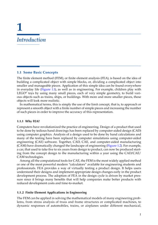
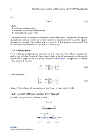
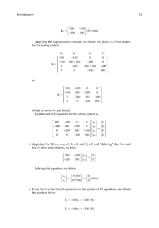
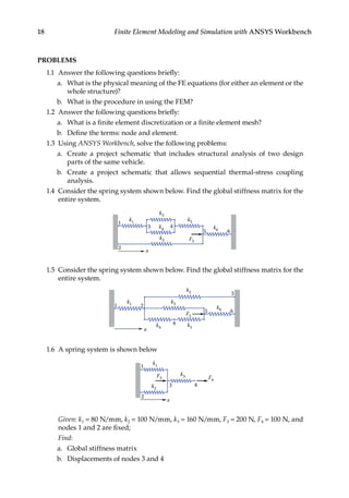
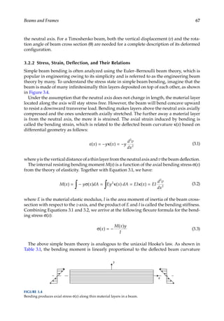
EXAMPLE 1.2
k1
x
k2
4
2
3
k3
5
F2
F1
k4
1
1
2 3
4
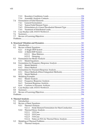
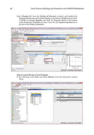
Problem
For the spring system with arbitrarily numbered nodes and elements, as shown above,
find the global stiffness matrix.
Solution
First, we construct the following element connectivity table:
Element Node i (1) Node j (2)
1 4 2
2 2 3
3 3 5
4 2 1
This table specifies the global node numbers corresponding to the local node numbers
for each element.

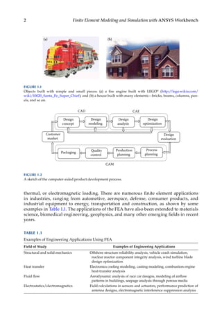
28. 13
Introduction
Then we write the element stiffness matrix for each element
u u
k k
k k
u u
k k
k k
u u
k
4 2
1
1 1
1 1
2 3
2
2 2
2 2
3 5
3
3
k
k
k
=
−
−






=
−
−






=
−
,
,
k
k
k k
u u
k k
k k
3
3 3
2 1
4
4 4
4 4
−






=
−
−






,
k
Finally, applying the superposition method, we obtain the global stiffness matrix as
follows:
u u u u u
k k
k k k k k k
k k k k
k k
1 2 3 4 5
4 4
4 1 2 4 2 1
2 2 3 3
1 1
0 0 0
0
0 0
0 0
K =
−
− + + − −
− + −
− 0
0
0 0 0
3 3
−
















k k
The matrix is symmetric, banded, but singular, as it should be.
After introducing the basic concepts, the section below introduces you to one of the
general-purpose finite element software tools—ANSYS Workbench.
1.3 Overview of ANSYS Workbench
ANSYS Workbench is a simulation platform that enables users to model and solve a wide
range of engineering problems using the FEA. It provides access to the ANSYS family
of design and analysis modules in an integrated simulation environment. This section
gives a brief overview of the different elements in the ANSYS Workbench simulation envi-
ronment or the graphical-user interface (GUI). Readers are referred to ANSYS Workbench
user’s guide [2] for more detailed information.
1.3.1 The User Interface
The Workbench interface is composed primarily of a Toolbox region and a Project Schematic
region (Figure 1.8). The main use of the two regions is described next.

29. 14 Finite Element Modeling and Simulation with ANSYS Workbench
1.3.2 The Toolbox
The Toolbox contains the following four groups of systems:
Analysis Systems: Predefined analysis templates to be used to build your project,
including static structural, steady-state thermal, transient thermal, fluid flow,
modal, shape optimization, linear buckling, and many others.
Component Systems: Component applications that can be used to build or expand an
analysis system, including geometry import, engineering data, mesh, postpro-
cessing, and others.
Custom Systems: Coupled-field analysis systems such as fluid solid interaction, pre-
stress modal, thermal-stress, and others.
Design Exploration: Parametric optimization studies such as response surface optimi-
zation, parameters correlation, six sigma analysis, and others.
1.3.3 The Project Schematic
A project schematic, that is, a graphical representation of the workflow, can be built by
dragging predefined analysis templates or other components from the Toolbox and drop-
ping them into the Project Schematic window. “Drag” here means to move the mouse while
holding down the left mouse button, and “drop” means to release the mouse button.
To build a project for static structural analysis, for instance, drag the Static Structural
template from the Toolbox and drop it into the rectangular box that appears in the Project
Schematic window. A standalone analysis system that contains the components needed for
static structural analysis is added to the project schematic as shown in Figure 1.9a. The
system consists of seven individual components called cells.
Alternatively, a standalone analysis can be created by double-clicking. For example,
double-click the Steady-State Thermal template from the Toolbox, and an independent
FIGURE 1.8
ANSYS Workbench user interface.

30. 15
Introduction
Steady-State Thermal system will be placed in the default location below the existing Static
Structural system, as shown in Figure 1.9b.
A system can be moved around another system in the project schematic. To move a sys-
tem, click on the header cell (i.e., the cell titled Steady-State Thermal for the thermal system)
and drag it to a new place. Once you drag the header cell, dashed rectangles appear for the
possible new locations to drop the system. This is illustrated in Figures 1.9c and d for two
systems with initial top–bottom and side-by-side configurations, respectively.
To delete a system, click on the down arrow button at the upper left corner of the system
from the Project Schematic window, and then choose Delete from the drop-down context
menu.
In some cases, a project may contain two or more analysis systems that share data. For
example, a downstream modal analysis may use the same material, geometry, and model
data from the preceding structural analysis. To build such a project, create a standalone
system for Static Structural analysis. Then, drag the Modal analysis template from the
Toolbox and drop it onto the Model cell of the Static Structural system. Immediately before
the subsequent system is dropped, bounding boxes will appear on the Engineering Data,
Geometry, and Model cells of the first system, as shown in Figure 1.10a. After the system
is released, a project including two linked systems is created, as shown in Figure 1.10b,
where the linked cells indicate data sharing at the Model and above levels.
FIGURE 1.9
Defining standalone analysis systems in the project schematic: (a) a standalone system; (b) two independent
standalone systems; (c) moving a system in a top-bottom configuration; and (d) moving a system in a side-by-
side configuration.

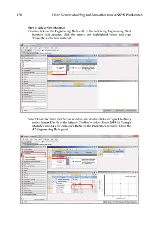
31. 16 Finite Element Modeling and Simulation with ANSYS Workbench
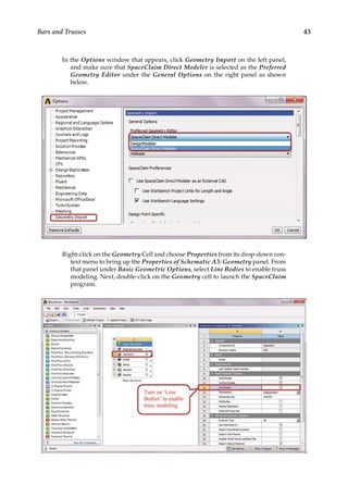
1.3.4 Working with Cells
Cells are components that make up an analysis system. You may launch an application by
double-clicking a cell. To initiate an action other than the default action, right-click on a
cell to view its context menu options. The following list comprises the types of cells avail-
able in ANSYS Workbench and their intended functions:
Engineering Data: Define or edit material models to be used in an analysis.
Geometry: Create, import, or edit the geometry model used for analysis.
Model/Mesh: Assign material, define coordinate system, and generate mesh for the
model.
Setup: Apply loads, boundary conditions, and configure the analysis settings.
Solution: Access the model solution or share solution data with other downstream
systems.
Results: Indicate the results availability and status (also referred to as postprocessing).
As the data flows through a system, a cell’s state can quickly change. ANSYS Workbench
provides a state indicator icon placed on the right side of the cell. Table 1.2 describes the
indicator icons and the various cell states available in ANSYS Workbench. For more infor-
mation, please refer to ANSYS Workbench user’s guide [2].
1.3.5 The Menu Bar
The menu bar is the horizontal bar anchored at the top of the Workbench user interface. It
provides access to the following functions:
File Menu: Create a new project, open an existing project, save the current project,
and so on.
View Menu: Control the window/workspace layout, customize the toolbox, and so on.
Tools Menu: Update the project and set the license preferences and other user options.
Units Menu: Select the unit system and specify unit display options.
Help Menu: Get help for ANSYS Workbench.
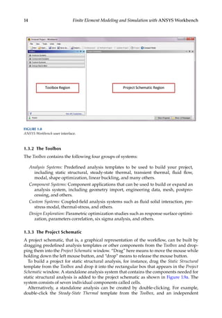
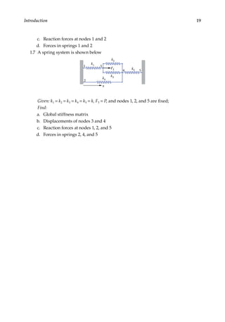
FIGURE 1.10
Defining linked analysis systems in the project schematic: (a) dropping the second (subsequent) system onto
the Model cell of the first system to share data at the model and above levels; (b) two systems that are linked.

32. 17
Introduction
In the chapters that follow, the use of ANSYS Workbench will be presented in a step-by-
step fashion in the context of real-world problem solving that may involve different mod-
eling concepts or different physics. It is worth noting that, although a commercial finite
element program enables you to deal with a wide range of engineering problems with
complex geometry, constraints, and material behaviors, it is your responsibility to under-
stand the underlying physics to be able to setup a problem correctly. Your FEA results, no
matter how pretty they may look, are only as good as the assumptions and decisions you
have made in building your model.
1.4 Summary
In this chapter, the basic concepts in the FEM are introduced. The spring system is used
as an example to show how to establish the element stiffness matrices, to assemble
the finite element equations for a system from element stiffness matrices, and to solve
the FE equations. Verifying the FE results is emphasized. ANSYS Workbench environ-
ment is briefly introduced. The concepts and procedures introduced in this chapter are
very simple and yet very important for studying the finite element analyses of other
problems.
TABLE 1.2
Indicator Icons and Descriptions of the Various Cell States
Cell State Indicator Description
Unfulfilled Need upstream data to proceed
Refresh required A refresh action is needed as a result of changes made on
upstream data
Attention required User interaction with the cell is needed to proceed
Update required An update action is needed as a result of changes made on
upstream data
Up to date Data are up to date and no attention is required
Input changes pending An update or refresh action is needed to recalculate based
on changes made to upstream cells
Interrupted Solution has been interrupted. A resume or update action
will make the solver continue from the interrupted point
Pending Solution is in progress
Source: Courtesy of ANSYS Workbench User’s Guide, Release 14.5, ANSYS, Inc., 2012.

33. 18 Finite Element Modeling and Simulation with ANSYS Workbench
PROBLEMS
1.1 Answer the following questions briefly:
a. What is the physical meaning of the FE equations (for either an element or the
whole structure)?
b. What is the procedure in using the FEM?
1.2 Answer the following questions briefly:
a. What is a finite element discretization or a finite element mesh?
b. Define the terms: node and element.
1.3 Using ANSYS Workbench, solve the following problems:
a. Create a project schematic that includes structural analysis of two design
parts of the same vehicle.
b. Create a project schematic that allows sequential thermal-stress coupling
analysis.
1.4 Consider the spring system shown below. Find the global stiffness matrix for the
entire system.
k1
x
k3
F5
k2
2
1
3 4
k4
k5
k6
5 6
1.5 Consider the spring system shown below. Find the global stiffness matrix for the
entire system.
k1
x
k3
F5
k2
2
1
3
5
k4 k5
k6
4
6
1.6 A spring system is shown below
k1
x
k3 F4
k2
F3
2
1
3 4
Given: k1 = 80 N/mm, k2 = 100 N/mm, k3 = 160 N/mm, F3 = 200 N, F4 = 100 N, and
nodes 1 and 2 are fixed;
Find:
a. Global stiffness matrix
b. Displacements of nodes 3 and 4

34. 19
Introduction
c. Reaction forces at nodes 1 and 2
d. Forces in springs 1 and 2
1.7 A spring system is shown below
k1
x
k3
k4
F3
k2
k5
2
1 3
4 5
Given: k1 = k2 = k3 = k4 = k5 = k, F3 = P, and nodes 1, 2, and 5 are fixed;
Find:
a. Global stiffness matrix
b. Displacements of nodes 3 and 4
c. Reaction forces at nodes 1, 2, and 5
d. Forces in springs 2, 4, and 5

36. 21
2
Bars and Trusses
2.1 Introduction
This chapter introduces you to the simplest one-dimensional (1-D) structural element,
namely the bar element, and the FEA of truss structures using such element. Trusses
are commonly used in the design of buildings, bridges, and towers (Figure 2.1). They are
triangulated frameworks composed of slender bars whose ends are connected through
bolts, pins, rivets, and so on. Truss structures create large, open, and uninterrupted space,
and offer lightweight and economical solutions to many engineering situations. If a truss,
along with the applied load, lies in a single plane, it is called a planar truss. If it has mem-
bers and joints extending into the three-dimensional (3-D) space, it is then a space truss.
Most structural analysis problems such as stress and strain analysis can be treated as
linear static problems, based on the following assumptions:
1. Small deformations (loading pattern is not changed due to the deformed shape)
2. Elastic materials (no plasticity or failures)
3. Static loads (the load is applied to the structure in a slow or steady fashion)
Linear analysis can provide most of the information about the behavior of a structure,
and can be a good approximation for many analyses. It is also the basis of nonlinear FEA
in most of the cases. In Chapters 2 through 7, only linear static responses of structures are
considered.
2.2 Review of the 1-D Elasticity Theory
We begin by examining the problem of an axially loaded bar based on 1-D linear elasticity.
Consider a uniform prismatic bar shown in Figure 2.2. The parameters L, A, and E are the
length, cross-sectional area, and elastic modulus of the bar, respectively.
Let u, ε, and σ be the displacement, strain, and stress, respectively (all in the axial direc-
tion and functions of x only), we have the following basic relations:
Strain–displacement relation:
ε =
( )
( )
x
du x
dx
(2.1)

37. 22 Finite Element Modeling and Simulation with ANSYS Workbench
Stress–strain relation:
σ = ε
( ) ( )
x E x (2.2)
Equilibrium equation:
d x
dx
f x
σ
+ =
( )
( ) 0 (2.3)
where f(x) is the body force (force per unit volume, such as gravitational and magnetic
forces) inside the bar. To obtain the displacement, strain, and stress field in a bar, Equations
2.1 through 2.3 need to be solved under given boundary conditions, which can be done
readily for a single bar, but can be tedious for a network of bars or a truss structure made
of many bars.
2.3 Modeling of Trusses
For the truss analysis, it is often assumed that: (1) the bar members are of uniform cross
sections and are joined together by frictionless pins, and (2) loads are applied to joints only
and not in between joints along the truss members. It is based on these assumptions that
the truss members are considered to carry only axial loads and have negligible bending
resistance.
x P
L
A, E
FIGURE 2.2
An axially loaded elastic bar.
FIGURE 2.1
Truss examples: (a) Montreal Biosphere Museum (http://en.wikipedia.org/wiki/Montreal_Biosph%C3%A8re).
(b) Betsy Ross Bridge (http://en.wikipedia.org/wiki/Betsy_Ross_Bridge).

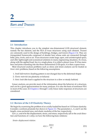
38. 23
Bars and Trusses
Given the fact that a truss is an assembly of axial bars, it is generally satisfactory to treat
each truss member as a discrete element—bar element. A bar element is a 1-D finite ele-
ment to describe the deformation, strain, and stress in a slender structure member that
often has a uniform cross section and is loaded in tension or compression only along its
axis.
Let us take a planar roof structure as an example to illustrate the truss model idealiza-
tion process. In an actual structure pictured in Figure 2.3a, purlins are used to support
the roof and they further transmit the load to gusset plates that connect the members.
In the idealized model shown in Figure 2.3b, each truss member is simply replaced by a
two-node bar element. A joint condition is modeled by node sharing between elements
connected end-to-end, and loads are imposed only on nodes. Components such as purlins
and gussets are neglected to avoid construction details that do not contribute significantly
to the overall truss load–deflection behavior. Other factors such as the weight of the truss
members can be considered negligible, compared to the loads they carry. If it were to be
included, a member’s weight can always be applied to its two ends, half the weight at each
end node. Experience has shown that the deformation and stress calculations for such
idealized models are often sufficient for the overall design and analysis purposes of truss
structures [3].
2.4 Formulation of the Bar Element
In this section, we will formulate the equations for the bar element based on the 1-D elas-
ticity theory. The structural behavior of the element, or the element stiffness matrix, can be
established using two approaches: the direct approach and the energy approach. The two
methods are discussed in the following.
2.4.1 Stiffness Matrix: Direct Method
A bar element with two end nodes is presented in Figure 2.4.
(a)
(b)
Roof
Purlin
Gusset
FIGURE 2.3
Modeling of a planar roof truss: (a) Physical structure. (b) Discrete model.

39. 24 Finite Element Modeling and Simulation with ANSYS Workbench
Assuming that the displacement u is varying linearly along the axis of the bar, that is, in
terms of the two nodal values ui and uj, we can write
u x
x
L
u
x
L
u
i j
( ) = −





 +
1 (2.4)
We have
ε =
−
= =
u u
L L
j i ∆
∆
( )
elongation (2.5)
σ = ε =
E
E
L
∆
(2.6)
We also have
σ = =
F
A
F
( )
force in bar (2.7)
Thus, Equations 2.6 and 2.7 lead to
F
EA
L
k
= =
∆ ∆
where k = EA/L is the stiffness of the bar. That is, the bar behaves like a spring in this case
and we conclude that the element stiffness matrix is
k =
−
−





 =
−
−












k k
k k
EA
L
EA
L
EA
L
EA
L
or
k =
−
−






EA
L
1 1
1 1
(2.8)
L
x
fi i j fj
ui
uj
A, E
FIGURE 2.4
Notation for a bar element.

40. 25
Bars and Trusses
This can be verified by considering the equilibrium of the forces at the two nodes.
The Element equilibrium equation is
EA
L
u
u
f
f
i
j
i
j
1 1
1 1
−
−













=







(2.9)
Degree of Freedom (DOF): Number of components of the displacement vector at a node.
For 1-D bar element along the x-axis, we have one DOF at each node.
Physical Meaning of the Coefficients in k: The jth column of k (here j = 1 or 2) represents the
forces applied to the bar to maintain a deformed shape with unit displacement at node j
and zero displacement at the other node.
2.4.2 Stiffness Matrix: Energy Approach
We derive the same stiffness matrix for the bar using a formal approach which can be
applied to many other more complicated situations.
First, we define two linear shape functions as follows (Figure 2.5):
N N
i j
( ) , ( )
ξ = − ξ ξ = ξ
1 (2.10)
where
ξ = ≤ ξ ≤
x
L
, 0 1 (2.11)
From Equation 2.4, we can write the displacement as
u x u N u N u
i i j j
( ) ( ) ( ) ( )
= ξ = ξ + ξ
or
u N N
u
u
i j
i
j
= 
 








= Nu (2.12)
Strain is given by Equations 2.1 and 2.12 as
ε = =





 =
du
dx
d
dx
N u Bu (2.13)
i j ξ
ξ = 0 ξ = 1 ξ = 1
ξ
Ni(ξ) Nj(ξ)
1
i j
ξ = 0
1
FIGURE 2.5
The shape functions for a bar element.

41. 26 Finite Element Modeling and Simulation with ANSYS Workbench
where B is the element strain–displacement matrix, which is
B = ξ ξ

 
 =
ξ
ξ ξ

 
 ⋅
ξ
d
dx
N N
d
d
N N
d
dx
i j i j
( ) ( ) ( ) ( )
that is,
B = −

 

1 1
/ /
L L (2.14)
Stress can be written as
σ = ε =
E EBu (2.15)
Consider the strain energy stored in the bar
U = σ ε =
=








∫ ∫
∫
1
2
1
2
1
2
T T T
T T
u B Bu
u B B u
V V
V
dV E dV
E dV
( )
( ) (2.16)
where Equations 2.13 and 2.15 have been used.
The potential of the external forces is written as (this is by definition, and remember the
negative sign)
Ω = − − = −
f u f u
i i j j u f
T
(2.17)
The total potential of the system is
Π = U + Ω
which yields by using Equations 2.16 and 2.17
Π =








−
∫
1
2
u B B u u f
T T T
( )
E dV
V
(2.18)
Setting dΠ = 0 by the principle of minimum potential energy, we obtain (verify this)
B B u f
T
E dV
V
( )








=
∫
or
ku = f (2.19)

42. 27
Bars and Trusses
where
k B B
T
=
∫( )
E dV
V
(2.20)
is the element stiffness matrix.
Equation 2.20 is a general result which can be used for the construction of other types
of elements.
Now, we evaluate Equation 2.20 for the bar element by using Equation 2.14
k =
−






−

 
 =
−
−






∫
1
1
1 1
1 1
1 1
0
/
/
/ /
L
L
E L L Adx
EA
L
L
which is the same as we derived earlier using the direct method.
Note that from Equations 2.16 and 2.20, the strain energy in the element can be written as
U =
1
2
u ku
T
(2.21)
In the future, once we obtain an expression like Equation 2.16, we can immediately rec-
ognize that the matrix in between the displacement vectors is the stiffness matrix. Recall
that for a spring, the strain energy can be written as
U = =
1
2
1
2
2
k k
T
∆ ∆ ∆
Thus, result (2.21) goes back to the simple spring case again.
2.4.3 Treatment of Distributed Load
Distributed axial load q (N/mm, N/m, lb/in) (Figure 2.6) can be converted into two
­
equivalent nodal forces using the shape functions. Consider the work done by the distrib-
uted load q,
W u x q x dx q x dx u u
N x
N x
q
L
T
L
i j
i
j
= = ( ) = 
 



∫ ∫
1
2
1
2
1
2
0 0
( ) ( ) ( )
( )
( )
Nu 




=
∫
∫
q x dx
q x dx
L
T T
L
( )
( )
0
0
1
2
u N (2.22)
x
i j
q
i j
fj
q
fi
q
FIGURE 2.6
Conversion of a distributed load on one element.

43. 28 Finite Element Modeling and Simulation with ANSYS Workbench
The work done by the equivalent nodal forces are
W f u f u
f i
q
i j
q
j
T
q
q = + =
1
2
1
2
1
2
u f (2.23)
Setting W W
q fq
= and using Equations 2.22 and 2.23, we obtain the equivalent nodal force
vector
f N
q
i
q
j
q
T
L
i
j
L
f
f
q x dx
N x
N x
q x dx
=










= =






∫ ∫
( )
( )
( )
( )
0 0
(2.24)
which is valid for any distributions of q. For example, if q is a constant, we have
fq
L
q
x L
x L
dx
qL
qL
=
−





 =






∫
1 2
2
0
/
/
/
/ (2.25)
that is, equivalent nodal forces can be added to replace the distributed load as shown in
Figure 2.7.
2.4.4 Bar Element in 2-D and 3-D
To analyze the truss structures in 2-D or 3-D, we need to extend the 1-D bar element for-
mulation to 2-D or 3-D. In the following, we take a look at the formulation for the 2-D case.
2.4.4.1 2-D Case
Local Global
x, y X, Y
′ ′
u v
i i
, ui, vi
1 DOF at each node 2 DOFs at each node
Note that lateral displacement ′
vi does not contribute to the stretch of the bar within the
linear theory (Figure 2.8). Displacement vectors in the local and global coordinates are
related as follows:
1 3
q
qL/2
1 3
qL/2
2
2
qL
FIGURE 2.7
Conversion of a distributed load with constant intensity q on two elements.

44. 29
Bars and Trusses
u u v l m
u
v
v u v m l
i i i
i
i
i
i
i i
′
= θ + θ = 
 







= − θ + θ = −


cos sin
sin cos 








u
v
i
i
where l = cos θ, m = sin θ.
In matrix form,
u
v
l m
m l
u
v
i
i
i
i
′
′










=
−












(2.26)
or,
u Tu
i i
′
=
where the transformation matrix
T =
−






l m
m l
(2.27)
is orthogonal, that is,
T T
−
=
1 T
.
For the two nodes of the bar element, we have
u
v
u
v
l m
m l
l m
m l
u
i
i
j
j
′
′
′
′














=
−
−












0 0
0 0
0 0
0 0
i
i
i
j
j
v
u
v














(2.28)
or,
′ = =








u Tu T
T 0
0 T
with
(2.29)
x
i
j
ui′
y
X
Y
θ
ui
vi
FIGURE 2.8
Local and global coordinates for a bar in 2-D space.

45. 30 Finite Element Modeling and Simulation with ANSYS Workbench
The nodal forces are transformed in the same way,
f′ = Tf (2.30)
In the local coordinate system, we have
EA
L
u
u
f
f
i
j
i
j
1 1
1 1
−
−
















=










′
′
′
′
Augmenting this equation, we write
EA
L
u
v
u
v
i
i
j
j
1 0 1 0
0 0 0 0
1 0 1 0
0 0 0 0
−
−

























′
′
′
′ 

=














′
′
f
f
i
j
0
0
or,
k′ u′ = f′
Using transformations given in Equations 2.29 and 2.30, we obtain
k′ Tu = Tf
Multiplying both sides by TT and noticing that TTT = I, we obtain
TT k′ Tu = f (2.31)
Thus, the element stiffness matrix k in the global coordinate system is
k = TT k′ T (2.32)
which is a 4 × 4 symmetric matrix.
Explicit form is
u v u
EA
L
l lm l lm
lm m lm m
l lm l lm
lm m lm m
i i j j
v
k =
− −
− −
− −
− −





2 2
2 2
2 2
2 2










(2.33)
Calculation of the directional cosines l and m:
l
X X
L
m
Y Y
L
j i j i
= =
−
= θ =
−
cos , sin
θ

46. 31
Bars and Trusses
The structure stiffness matrix is assembled by using the element stiffness matrices in the
usual way as in the 1-D case.
2.4.4.2 3-D Case
Local Global
x, y, z X, Y, Z
′ ′ ′
u v w
i i i
, , ui, vi, wi
1 DOF at each node 3 DOFs at each node
Similar to the 2-D case, element stiffness matrices in the 3-D case are calculated in the
local coordinate systems first and then transformed into the global coordinate system (X,
Y, and Z) where they are assembled (Figure 2.9). The transformation relation is
u
v
w
l l l
m m m
n n n
u
v
w
i
i
i
X Y Z
X Y Z
X Y Z
i
i
i
′
′
′










=





















(2.34)
where (lX,lY,lZ), (mX,mY,mZ), and (nX,nY,nZ) are the direction cosines of the local x, y, and z
coordinate axis in the global coordinate system, respectively. FEM software packages will
do this transformation automatically.
Therefore, the input data for bar elements are simply:
• Coordinates (X, Y, Z) for each node
• E and A for each element (length L can be computed from the coordinates of the
two nodes)
2.4.5 Element Stress
Once the nodal displacement is obtained for an element, the stress within the element can
be calculated using the basic relations. For example, for 2-D cases, we proceed as follows:
σ = ε =










= −












′
′
E E
u
u
E
L L
l m
l m
u
v
u
v
i
j
i
i
j
j
B
1 1 0 0
0 0















x
i
j
y
X
Y
Z
z
FIGURE 2.9
Local and global coordinates for a bar in 3-D space.

47. 32 Finite Element Modeling and Simulation with ANSYS Workbench
That is,
σ = − −

 















E
L
l m l m
u
v
u
v
i
i
j
j
(2.35)
which is a general formula for 2-D bar elements.
2.5 Examples with Bar Elements
We now look at examples of using the bar element in the analysis of 1-D stress problems
and plane truss problems.
EXAMPLE 2.1
x
1 2
3
L
A, E
2A, E
P
1 2
L
Problem
Find the stresses in the two-bar assembly which is loaded with force P, and constrained
at the two ends, as shown in the above figure.
Solution
Use two 1-D bar elements.
For element 1,
u u
EA
L
1 2
1
2 1 1
1 1
k =
−
−






For element 2,
u u
EA
L
2 3
2
1 1
1 1
k =
−
−






Imagine a frictionless pin at node 2, which connects the two elements. We can assem-
ble the global FE equation as follows:

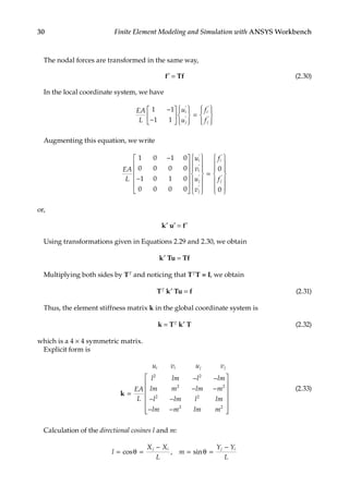
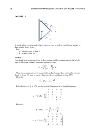
48. 33
Bars and Trusses
EA
L
u
u
u
F
F
F
2 2 0
2 3 1
0 1 1
1
2
3
1
2
3
−
− −
−




















=











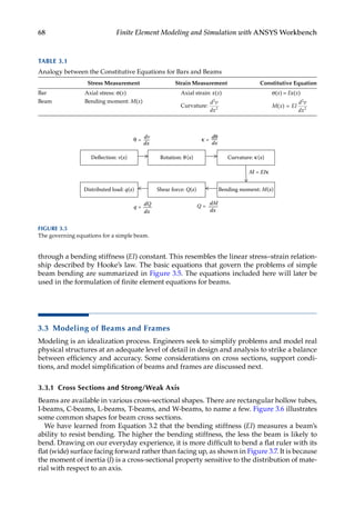
Load and boundary conditions (BCs) are
u u F P
1 3 2
0
= = =
,
FE equation becomes
EA
L
u
F
P
F
2 2 0
2 3 1
0 1 1
0
0
2
1
3
−
− −
−




















=










“Deleting” the first row and column, and the third row and column, we obtain
EA
L
u P
3 2
[ ]{ } = { }
Thus,
u
PL
EA
2
3
=
and
u
u
u
PL
EA
1
2
3
3
0
1
0










=










Stress in element 1 is
σ = ε = = −

 








=
−
= −




1 1 1 1
1
2
2 1
1 1
3
0
E E E L L
u
u
E
u u
L
E
L
PL
EA
B u / /


 =
P
A
3
Similarly, stress in element 2 is
σ = ε = = −

 








=
−
= −




2 2 2 2
2
3
3 2
1 1
0
3
E E E L L
u
u
E
u u
L
E
L
PL
EA
B u / /


 = −
P
A
3
which indicates that bar 2 is in compression.

49. 34 Finite Element Modeling and Simulation with ANSYS Workbench
Check the results: Draw the FBD as follows and check the equilibrium of the
structures.
P –P/3
–2P/3
Notes:
• In this case, the calculated stresses in elements 1 and 2 are exact. It will not
help if we further divide element 1 or 2 into smaller elements.
• For tapered bars, averaged values of the cross-sectional areas should be used
for the elements.
• We need to find the displacements first in order to find the stresses, and this
approach is called the displacement-based FEM.
EXAMPLE 2.2
x
Δ
1 2 3
L
L
A, E
P
1 2
Problem
Determine the support reaction forces at the two ends of the bar shown above, given
the following:
P E
A L =
= × = ×
= =
6 0 10 2 0 10
250 150
4 4
2
. , . ,
,
N N/mm
mm mm, 1.2 mm
2
∆
Solution
We first check to see if contact of the bar with the wall on the right will occur or not. To
do this, we imagine the wall on the right is removed and calculate the displacement at
the right end
∆ ∆
0
4
4
6 0 10 150
2 0 10 250
1 8 1 2
= =
×
×
= =
PL
EA
( . )( )
( . )( )
. .
mm mm
Thus, contact occurs and the wall on the right should be accounted for in the analysis.
The global FE equation is found to be
EA
L
u
u
u
F
F
F
1 1 0
1 2 1
0 1 1
1
2
3
1
2
3
−
− −
−




















=












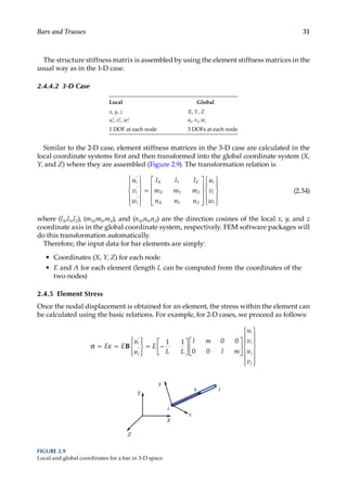
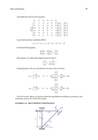
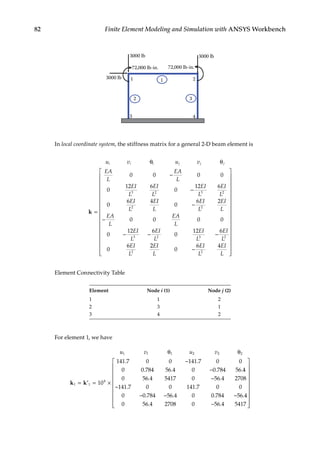
50. 35
Bars and Trusses
The load and boundary conditions are
F P
u u
2
4
1 3
6 0 10
0 1 2
= = ×
= = =
.
, .
N
mm
∆
The FE equation becomes
EA
L
u
F
P
F
1 1 0
1 2 1
0 1 1
0
2
1
3
−
− −
−




















=










∆
The second equation gives
EA
L
u
P
2 1
2
−

 








= { }
∆
that is,
EA
L
u P
EA
L
2 2
[ ]{ } = +






∆
Solving this, we obtain
u
PL
EA
2
1
2
1 5
= +





 =
∆ . mm
and
u
u
u
1
2
3
0
1 5
1 2










=










.
.
( )
mm
To calculate the support reaction forces, we apply the first and third equations in the
global FE equation.
The first equation gives
F
EA
L
u
u
u
EA
L
u
1
1
2
3
2
4
1 1 0 5 0 10
= −

 











= −
( ) = − ×
. N
and the third equation gives,
F
EA
L
u
u
u
EA
L
u u
3
1
2
3
2 3
4
0 1 1 1 0 10
= −

 











= − +
( ) = − ×
. N
Check the results: Again, we can draw the free-body diagram to verify that the equilib-
rium of the forces is satisfied.

51. 36 Finite Element Modeling and Simulation with ANSYS Workbench
EXAMPLE 2.3
X
Y P1
P2
45°
45°
3
2
1
1
2
A simple plane truss is made of two identical bars (with E, A, and L), and loaded as
shown in the above figure.
Find
a. displacement of node 2;
b. stress in each bar.
Solution
This simple structure is used here to demonstrate the FEA procedure using the bar ele-
ment in 2-D space. In local coordinate systems, we have
k k
1 2
1 1
1 1
′ ′
=
−
−





 =
EA
L
These two matrices cannot be assembled together, because they are in different coor-
dinate systems. We need to convert them into global coordinate system OXY.
Element 1:
θ = = =
45
2
2
o
, l m
Using Equation 2.32 or 2.33, we obtain the stiffness matrix in the global system
u v u v
EA
L
T
1 1 2 2
1 1 1 1
2
1 1 1 1
1 1 1 1
1 1 1 1
1 1 1 1
k T k T
= =
− −
− −
− −
− −










′ 




Element 2:
θ = = − =
135
2
2
2
2
o
, ,
l m
u v u v
EA
L
T
2 2 3 3
2 2 2 2
2
1 1 1 1
1 1 1 1
1 1 1 1
1 1 1 1
k T k T
= ′
=
− −
− −
− −
− −
















52. 37
Bars and Trusses
Assemble the structure FE equation,
u v u v u v
EA
L
1 1 2 2 3 3
2
1 1 1 1 0 0
1 1 1 1 0 0
1 1 2 0 1 1
1 1 0 2 1 1
0 0 1 1 1 1
− −
− −
− − −
− − −
− −
0
0 0 1 1 1 1
1
1
2
2
3
3
− −




































=
u
v
u
v
u
v
F
F
F
F
F
F
F
X
Y
X
Y
X
Y
1
1
2
2
3
3


















Load and boundary conditions (BCs):
u v u v F P F P
X Y
1 1 3 3 2 1 2 2
0
= = = = = =
, ,
Condensed FE equation,
EA
L
u
v
P
P
2
2 0
0 2
2
2
1
2













=







Solving this, we obtain the displacement of node 2,
u
v
L
EA
P
P
2
2
1
2







=







Using Equation 2.34, we calculate the stresses in the two bars,
σ = − −

 















= +
( )
1
1
2
1 2
2
2
1 1 1 1
0
0 2
2
E
L
L
EA P
P
A
P P
σ = − −

 















= −
( )
2
1
2
1 2
2
2
1 1 1 1
0
0
2
2
E
L
L
EA
P
P
A
P P
Check the results: Again, we need to check the equilibrium conditions, symmetry, anti-
symmetry, and so on, of the FEA results.
EXAMPLE 2.4: (MULTIPOINT CONSTRAINT)
X
Y
P
45°
3
2
1
3
2
1
x′
y′
L

53. 38 Finite Element Modeling and Simulation with ANSYS Workbench
For the plane truss shown above,
P L m E GPa
A m
= = =
= × −
1000 1 210
6 0 10 4 2
kN,
for elements 1 and
, ,
. 2,
for element 3.
A m
= × −
6 2 10 4 2
Determine the displacements and reaction forces.
Solution
We have an inclined roller at node 3, which needs special attention in the FE solution.
We first assemble the global FE equation for the truss.
Element 1:
θ = = =
90 0 1
o
, ,
l m
u v u v
1 1 2 2
1
9 4
210 10 6 0 10
1
0 0 0 0
0 1 0 1
0 0 0 0
0 1 0 1
k =
× × −
−









−
( )( . )






( )
N/m
Element 2:
θ = = =
0 1 0
o
, ,
l m
u v u v
2 2 3 3
2
9 4
210 10 6 0 10
1
1 0 1 0
0 0 0 0
1 0 1 0
0 0 0 0
k =
× ×
−
−









−
( )( . )






( )
N/m
Element 3:
θ = = =
45
1
2
1
2
o
, ,
l m
u v u v
1 1 3 3
3
9 4
210 10 6 2 10
2
0 5 0 5 0 5 0 5
0 5 0 5 0 5 0 5
k =
× ×
− −
− −
−
( )( )
. . . .
. . . .
−
− −
− −














0 5 0 5 0 5 0 5
0 5 0 5 0 5 0 5
. . . .
. . . .
( )
N/m

54. 39
Bars and Trusses
The global FE equation is,
1260 10
0 5 0 5 0 0 0 5 0 5
1 5 0 1 0 5 0 5
1 0 1 0
1 0 0
1 5 0 5
0
5
×
− −
− − −
−
. . . .
. . .
. .
.
Sym. 5
5
1
1
2
2
3
3










































=
u
v
u
v
u
v
F1
1
1
2
2
3
3
X
Y
X
Y
X
Y
F
F
F
F
F






















Load and boundary conditions (BCs):
u v v v
F P F
X x
1 1 2 3
2 3
0 0
0
= = = ′ =
= =
′
, ,
, .
and
From the transformation relation and the BCs, we have
′
ν = −













= − + =
3
3
3
3 3
2
2
2
2
2
2
0
u
v
u v
( ) ,
that is,
u3 − v3 = 0
This is a multipoint constraint (MPC).
Similarly, we have a relation for the force at node 3,
F
F
F
F F
x
X
Y
X Y
3
3
3
3 3
2
2
2
2
2
2
0
′ =













= + =
( ) ,
that is,
F3X + F3Y = 0
Applying the load and BCs in the structure FE equation by “deleting” the first,
­
second, and fourth rows and columns, we have
1260 10
1 1 0
1 1 5 0 5
0 0 5 0 5
5
2
3
3
3
×
−
−




















=
. .
. .
u
u
P
F X
v F
F Y
3










Further, from the MPC and the force relation at node 3, the equation becomes,
1260 10
1 1 0
1 1 5 0 5
0 0 5 0 5
5
2
3
3
3
×
−
−




















=
. .
. .
u
u
u
P
F X
−
−










F X
3
which is
1260 10
1 1
1 2
0 1
5 2
3
3
3
×
−
−

















=
−










u
u
P
F
F
X
X
The third equation yields,
F u
X
3
5
3
1260 10
= − ×

55. 40 Finite Element Modeling and Simulation with ANSYS Workbench
Substituting this into the second equation and rearranging, we have
1260 10
1 1
1 3 0
5 2
3
×
−
−













=







u
u
P
Solving this, we obtain the displacements,
u
u
P
P
2
3
5
1
2520 10
3 0 01191
0 003968







=
×







=







.
.
( )
m
From the global FE equation, we can calculate the reaction forces,
F
F
F
F
F
X
Y
Y
X
Y
1
1
2
3
3
5
1260 10
0 0 5 0 5
0 0 5 0


















= ×
− −
− −
. .
. .
.
. .
. .
5
0 0 0
1 1 5 0 5
0 0 5 0 5
500
2
3
3
−


























=
−
u
u
v
−
−
−


















500
0 0
500
500
. ( )
kN
Check the results!
A general MPC can be described as,
A u
j j
j
=
∑ 0
where Aj’s are constants and uj’s are nodal displacement components. In FE software,
users only need to specify this relation to the software. The software will take care of
the solution process.
2.6 Case Study with ANSYS Workbench
Problem Description: Truss bridges can span long distances and support heavy weights
without intermediate supports. They are economical to construct and are available in a
wide variety of styles. Consider the following planar truss, constructed of wooden tim-
bers, which can be used in parallel to form bridges. Determine the deflections at each joint
of the truss under the given loading conditions.
Solution
To solve the problem with ANSYS Workbench, we employ the following steps:
Step 1: Start an ANSYS Workbench Project
Launch ANSYS Workbench and save the blank project as ‘Woodtruss.wbpj’.

56. 41
Bars and Trusses
Step 2: Create a Static Structural Analysis System
Drag the Static Structural icon from the Analysis Systems Toolbox at the left
and drop it inside the highlighted green rectangle in the Project Schematic to
create a standalone static structural analysis system.
Step 3: Add a New Material
Double-click (or right-click and choose Edit) on the Engineering Data cell in
the Project Schematic to edit or add a material. In the following Engineering
Data interface which replaces the Project Schematic, click the empty box
highlighted below and type a name, e.g., ‘Douglas Fir’, for the new material.
Note: If the Engineering Data interface fails to appear, click the View tab from the
top menu, and click Reset Workspace from the drop-down menu.

57. 42 Finite Element Modeling and Simulation with ANSYS Workbench
Select ‘Douglas Fir’ from the Outline of Schematic window, and double-click
Isotropic Elasticity under Linear Elastic in the leftmost Toolbox panel. Enter
‘1.31E10’ for Young’s Modulus and ‘0.29’ for Poisson’s Ratio in the bottom
center Properties of Outline window. Close the A2: Engineering Data tab to
go back to the Project Schematic.
Step 4: Launch the SpaceClaim Program
In the following, click Tools and select Options from the drop-down context
menu.

58. 43
Bars and Trusses
In the Options window that appears, click Geometry Import on the left panel,
and make sure that SpaceClaim Direct Modeler is selected as the Preferred
Geometry Editor under the General Options on the right panel as shown
below.
Right-click on the Geometry Cell and choose Properties from its drop-down con-
text menu to bring up the Properties of Schematic A3: Geometry panel. From
that panel under Basic Geometric Options, select Line Bodies to enable truss
modeling. Next, double-click on the Geometry cell to launch the SpaceClaim
program.

59. 44 Finite Element Modeling and Simulation with ANSYS Workbench
Step 5: Create Line Sketch
To customize units, click SpaceClaim Options from the File drop-down menu
shown below.

60. 45
Bars and Trusses
The following SpaceClaim Options window will show up. Click Units from the
left panel, and select Meters from the drop-down list of Length. Next, change
the Minor Grid Spacing to 1m. Click OK to save your changes and exit.

61. 46 Finite Element Modeling and Simulation with ANSYS Workbench
Next, click on Plan View in the mini-toolbar to display a head-on (top) view of
the sketch grid. Click on the Y symbol located at the bottom left corner in the
Graphics Window to display a bottom view of the sketch grid.
Alternatively, you may also select Bottom in the Views tab on the left to display
the same bottom view, as shown below.

62. 47
Bars and Trusses
Click the Sketch Mode icon on the Design tab to begin a sketch. Click on the Line
icon. To draw a line, click a start point and then an end point in the sketch grid.
When necessary, press the Esc key to end the line creation. Draw 13 lines as
shown below.
Modeling tips: Right-click anywhere in the Graphics Window, and click
View to switch between different standard views from the drop-down
menu.
To view your design from different angles, hover the mouse over the cen-
ter of the design, and press down the middle Scroll Wheel. You can see
a spin icon in the center, and simply move the mouse around to rotate the
view.
To move the object around the screen to pan it, press the Ctrl key and the Scroll
Wheel, and move the mouse around.
To zoom in and out of the design, press the Shift key and the Scroll Wheel, and
move the mouse around.
To come back to home view, simply press the H key.

63. 48 Finite Element Modeling and Simulation with ANSYS Workbench
Step 6: Create a Cross Section
Click Profiles on the Prepare tab, and select the Rectangle icon in the New Profile
Library from the Profiles drop-down menu.
A Beam Profiles folder is now added into the Structure Tree on the left. Right-
click on Rectangle under the Beam Profiles folder, and select Edit Beam
Profile from the drop-down context menu.

64. 49
Bars and Trusses
In the Driving Dimensions folder showing up next, click on B to bring up its
default Ruler dimension value. Click on the default Ruler dimension value,
and change it to 0.06m. Repeat the same step for H, and change the Ruler
dimension value for H to 0.06m as shown below in the Type column. Close the
SYS tab to return back to the Graphics Window for sketch modeling.
Step 7: Assign Cross Section to Line Sketch
Click Select on the Design tab, and select all 13 Lines under the Curves folder in
the Structure Tree. To select all lines in the tree, click the first Line in the struc-
ture tree, and hold the Shift key and click the last Line. The selected lines will
be highlighted in yellow as shown below.

65. 50 Finite Element Modeling and Simulation with ANSYS Workbench
Click Create on Prepare tab to create beams from the selected lines using the
rectangular cross-section provided.
This will bring up a Beams folder in the Structure Tree to replace the previous
Curves folder. The Beams folder contains 13 Beams (Rectangle) as shown
below.

66. 51
Bars and Trusses
Step 8: Move all Beams to a New Component
Click Select on the Design tab, and select all 13 Beams in the Structure Tree. To
select all beams in the tree, click the first Beam, and hold Shift key and click the
last Beam. The selected beams will be highlighted in yellow as shown below.
Right-click on the highlighted Beams in the Structure Tree in the above figure, and
selectMovetoNewComponentinthedrop-downcontextmenu.AComponent1
will be created in the Structure Tree with all 13 beams moved underneath.

67. 52 Finite Element Modeling and Simulation with ANSYS Workbench
Next, click Component1 in the Structure Tree, and change the Share Topology to
Merge in the bottom left Properties menu to merge all the beams. After that,
save and exit SpaceClaim.
Step 9: Launch the Static Structural Program
Double-click the Model cell to launch the Static Structural program. In the Static
Structural program that brings up, click Beam (Rectangle) under Geometry
in the Project Outline. Next, in the Details of “Beam (Rectangle)”, click to
the right of the Assignment field under Material, and select Douglas Fir from
the drop-down menu to replace the default material assignment of Structural
Steel.

68. 53
Bars and Trusses
Step 10: Generate Mesh
Click on Mesh in the Project Outline. In the Details of “Mesh”, enter a fairly
large number, say,’10’, for the Element Size. The value of the element size will
be set as 10m. This large element size value will ensure that each truss member
will be meshed with only one element. Next, right-click on Mesh in the Project
Outline, and select Generate Mesh.
The following mesh plot will show up. Click on Statistics in the Details of
“Mesh” to display the total number of nodes and elements in the mesh.

69. 54 Finite Element Modeling and Simulation with ANSYS Workbench
Step 11: Apply Boundary Conditions
Right-click on Static Structural (A5) in the Project Outline, and select Insert
and then Fixed Support. A Fixed Support item will be added underneath
Static Structural (A5) in the Project Outline.
Click on the Vertex filter icon to enable point selection, and select the two points
as shown below in the Graphics Window. In the Details of “Fixed Support”,
click Apply to confirm on the Geometry selection. After completion, a Fixed
Support boundary condition will be added to the selected two points.

70. 55
Bars and Trusses
Step 12: Apply Loads
Right-click on Static Structural (A5) in the Project Outline, and select Insert
and then Force.
Select the three points as shown below in the Graphics Window. In the Details
of “Force”, click Apply to confirm on the Geometry selection. Next, change the
Define By selection to Components and enter ‘-90000’ for Z Component in the
Details of “Force”. A downward red arrow will appear on the group of points
in the Graphics Window to represent the applied force.

71. 56 Finite Element Modeling and Simulation with ANSYS Workbench
Alternatively, the load can be applied to each of the three points separately
by inserting Force three times under Static Structural (A5) in the Project
Outline. In this case, enter ‘-30000’ for Z Component in the Details of “Force”
for each individual Force item.
Step 13: Retrieve Solution
Insert a Total Deformation item by right-clicking on Solution (A6) in the Project
Outline.
Right-click on Solution (A6) in the Outline tree and select Solve. The program
will start to solve the model.
After completion, click Total Deformation in the Outline to review the total
deformation results.

72. 57
Bars and Trusses
Modeling tips: To get the reaction force, a Force Reaction probe can be inserted
by right-clicking on Solution (A6) in the Outline tree as shown below.
In the Details of “Force Reaction”, select the Fixed Support as the Boundary
Condition.

73. 58 Finite Element Modeling and Simulation with ANSYS Workbench
Right-click on Solution (A6) in the Outline tree and select Evaluate All Results.
After completion, click Force Reaction in the Outline to review results.
Note here that the reaction force is found to be 90000 N in the positive Y-direction.
This is because a boundary condition has been applied earlier to the two fixed
ends in one step (see Step 11). To avoid summing of the force reaction, two fixed
conditions can be inserted instead in Step 11, one for each end. The reaction
forces at an individual support can then be displayed by selecting the support
of interest from the drop-down menu of Boundary Condition in the Details
of “Force Reaction”.

74. 59
Bars and Trusses
2.7 Summary
In this chapter, we studied the bar elements which can be used in truss analysis. The con-
cept of the shape functions is introduced and the derivations of the stiffness matrices using
the energy approach are introduced. Treatment of distributed loads is discussed and sev-
eral examples are studied. A planar truss structure is analyzed using ANSYS Workbench.
It provides basic modeling techniques and shows step-by-step how Workbench can be used
to determine the deformation and reaction forces in trusses.
2.8 Review of Learning Objectives
Now that you have finished this chapter you should be able to
1. Set up simplified finite element models for truss structures.
2. Derive the stiffness matrix for plane bar elements using direct and energy
approaches.
3. Explain the concept of shape functions and their characteristics for bar elements.
4. Find the equivalent nodal loads of distributed forces on bars.
5. Determine the displacement and stress of a truss using hand calculation to verify
the finite element solutions.
6. Apply the general bar element stiffness matrix to the analysis of simple trusses.
7. Create line sketches and new material definition in ANSYS Workbench.
8. Perform static structural analyses on trusses using ANSYS Workbench.
PROBLEMS
2.1 A bar assembly is loaded with force P at one end and constrained at the other
end, as shown in the figure below. Determine:
a. The displacement at node 2 and node 3
b. The stress in the bar assembly
P
1 2 3 4
L L
L
E, A
E, 2A
E, A
2.2 A simple structure with the profile shown below is loaded with force P, and
­
constrained at one end. Young’s modulus E is the same for all the bars. The
cross-sectional areas are shown in the figure. Use 1-D bar elements to approxi-
mate the deformation and the stresses in the structure.

75. 60 Finite Element Modeling and Simulation with ANSYS Workbench
P
5L 2L
2L
3A A 3A
A
5L
A
A
2.3 The plane truss is loaded with force P as shown below. Constants E and A for
each bar are as shown in the diagram. Determine:
a. The nodal displacements
b. The reaction forces
c. The stresses in bar elements
X
Y
3
2
1
L
L
E, A
E, A
4
L
E, A
P
2.4 The plane truss is loaded with force P as shown below. Constants E and A for
each bar are as shown in the diagram. Determine:
a. The nodal displacements
b. The reaction forces
c. The stresses in bar elements
X
Y
P
45°
3
2
1
L
45°
E, 2 A
2
E, A
E, A
L
4
2.5 The plane truss is loaded with force P as shown below. Constants E and A for
each bar are as shown in the diagram. Determine:
a. The nodal displacements
b. The stresses in bar elements

76. 61
Bars and Trusses
X
Y
P
45°
3
2
1
L
45°
E, 2 2A
E, A
E, A
2.6 The plane truss is supported as shown below. Young’s modulus E is the same
for all the bars. The cross-sectional areas are shown in the figure. Suppose that
the node 2 settles by an amount of δ as shown. Determine the stresses in each
bar element using the FEM.
X
Y
3
2
1
L
2 2 A
L
δ
A
A
2.7 The plane truss is loaded with force P as shown below. Young’s modulus E is
the same for all the bars. The cross-sectional areas are shown in the figure.
Determine:
a. The nodal displacements
b. The stresses in each bar element
X
Y
3
2
1
L
2
L
A
A
4
L
2 2A
A
P
2A
2.8 The plane truss is loaded with force P as shown below. Young’s modulus E is
the same for all the bars. The cross-sectional areas are shown in the figure.
Determine the nodal displacements and the reaction forces.

77. 62 Finite Element Modeling and Simulation with ANSYS Workbench
X
Y
4
2
1
L/2
L
A
2A
L
2A
P
5
3
L/2
2A
5A
5A
5A
2.9 The roof truss shown below is made of Douglas fir timbers of a 5 mm × 5 mm
cross section. Use ANSYS Workbench to determine the truss deformation and
the support reaction forces.
0.2 m 0.25 m 0.25 m 0.25 m 0.25 m 0.2 m
0.2 m
0.25 m
0.25 m
1 kN
1 kN
1 kN
1 kN
1 kN
2.10 The truss tower crane shown below is made of structural steel rectangular bars
of a 3 mm × 3 mm cross section. Use ANSYS Workbench to determine the truss
deformation and the support reaction forces.
0.1 m
0.1 m
0.1 m
0.2 m
0.5 m
0.5 m
0.5 m
0.5 m 0.5 m
0.5 m
0.5 m
0.5 m
6 kN
2.11 The truss bridge shown below is made of Douglas fir timbers of a 4 mm × 4 mm
cross section. Use ANSYS Workbench to determine the truss deformation and
the support reactions.

78. 63
Bars and Trusses
0.5 m 0.5 m 0.5 m 0.5 m 0.5 m 0.5 m
0.15 m
0.25 m
0.5 m
1.5 kN
1.5 kN
1.5 kN
1.5 kN
1.5 kN
2.12 The truss transmission tower shown below is made of structural steel members
of a 2.5 mm × 2.5 mm cross section. Use ANSYS Workbench to determine the
truss deformation and the support reactions.
0.6 m
0.8 m
0.8 m
1.2 m
1.8 m
1.5 kN
0.8 m 0.5 m 1 m 0.5 m 0.8 m
0.3 m
0.3 m
1.5 kN
1 kN
1 kN

80. 65
3
Beams and Frames
3.1 Introduction
Beams and frames are frequently used in constructions, in engineering equipment, and in
everyday life, for example, in buildings, lifting equipment, vehicles, and exercise machines
(Figure 3.1).
Beams are slender structural members subjected primarily to transverse loads. A beam
is geometrically similar to a bar in that its longitudinal dimension is significantly larger
than the two transverse dimensions. Unlike bars, the deformation in a beam is predomi-
nantly bending in transverse directions. Such a bending-dominated deformation is the
primary mechanism for a beam to resist transverse loads. In this chapter, we will use
the term “general beam” for a beam that is subjected to both bending and axial forces, and
the term “simple beam” for a beam subjected to only bending forces. The term “frame” is
used for structures constructed of two or more rigidly connected beams.
3.2 Review of the Beam Theory
We start with a brief review of the simple beam theory. Essential features of the two well-
known beam models, the Euler–Bernoulli beam and the Timoshenko beam, will be intro-
duced, followed by discussions on the stress, strain, and deflection relations in simple
beam theory.
3.2.1 Euler–Bernoulli Beam and Timoshenko Beam
Euler–Bernoulli beam and Timoshenko beam, as shown in Figure 3.2, are two common
models that are used in the structural analysis of beams and frames. Both models have at
their core the assumption of small deformation and linear elastic isotropic material behav-
ior. They are applicable to beams with uniform cross sections.
For a Euler–Bernoulli beam, it is assumed that the forces on a beam only cause the beam
to bend. There is no transverse shear deformation occurring in the beam bending. The
neutral axis, an axis that passes through the centroid of each beam cross section, does not
change in length after the deformation. A planar cross section perpendicular to the neu-
tral axis remains plane and perpendicular to the neutral axis after deformation. Due to its
neglect of shear strain effects, the Euler–Bernoulli model tends to slightly ­
underestimate

81. 66 Finite Element Modeling and Simulation with ANSYS Workbench
the beam deformation. The model is considered suitable for describing the behavior of
thin or long beams.
The Timoshenko beam model accounts for both transverse shear deformation and bend-
ing deformation. In this model, a planar cross section remains plane, but does not remain
normal to the neutral axis after deformation. By taking into account shear strain effects,
the Timoshenko model is physically more realistic for describing the behavior of thick or
short beams.
To determine the deflection of a laterally loaded beam of the same material and uniform
cross section, we may view the beam as a 1-D model with the transverse load assigned to
its neutral axis. As illustrated in Figure 3.3, for a Euler–Bernoulli beam, we need only one
variable—the vertical displacement (v), to describe the beam deflection at any point along
Deformed:
Reference:
Euler–Bernoulli beam Timoshenko beam
FIGURE 3.2
Two common beam models.
v v
=
Euler–Bernoulli beam
dv
dv
dx
dx
Timoshenko beam
90° 90°
θ
θ
FIGURE 3.3
Deflection of Euler–Bernoulli beam and Timoshenko beam.
FIGURE 3.1
Examples of beams and frames: (a) a car frame (http://www.carbasics-1950.com/); and (b) an exercise machine.
(From http://www.nibbledaily.com/body-by-jake-cardio-cruiser/.)

82. 67
Beams and Frames
the neutral axis. For a Timoshenko beam, both the vertical displacement (v) and the rota-
tion angle of beam cross section (θ) are needed for a complete description of its deformed
configuration.
3.2.2 Stress, Strain, Deflection, and Their Relations
Simple beam bending is often analyzed using the Euler–Bernoulli beam theory, which is
popular in engineering owing to its simplicity and is referred to as the engineering beam
theory by many. To understand the stress state in simple beam bending, imagine that the
beam is made of many infinitesimally thin layers deposited on top of each other, as shown
in Figure 3.4.
Under the assumption that the neutral axis does not change in length, the material layer
located along the axis will stay stress free. However, the beam will bend concave upward
to resist a downward transverse load. Bending makes layers above the neutral axis axially
compressed and the ones underneath axially stretched. The further away a material layer
is from the neutral axis, the more it is strained. The axial strain induced by bending is
called the bending strain, which is related to the deflected beam curvature κ(x) based on
differential geometry as follows:
ε = − κ = −
( ) ( )
x y x y
d v
dx
2
2
(3.1)
where y is the vertical distance of a thin layer from the neutral axis and v the beam deflection.
The internal resisting bending moment M(x) is a function of the axial bending stress σ(x)
from the theory of elasticity. Together with Equation 3.1, we have:
M x y x dA Ey x dA EI x EI
d v
dx
( ) ( ) ( ) ( )
= − σ = κ = κ =
∫ ∫ 2
2
2
(3.2)
where E is the material elastic modulus, I is the area moment of inertia of the beam cross-
section with respect to the z-axis, and the product of E and I is called the bending stiffness.
Combining Equations 3.1 and 3.2, we arrive at the following flexure formula for the bend-
ing stress σ(x):
σ = −
( )
( )
x
M x y
I
(3.3)
The above simple beam theory is analogous to the uniaxial Hooke’s law. As shown in
Table 3.1, the bending moment is linearly proportional to the deflected beam curvature
y
x
FIGURE 3.4
Bending produces axial stress σ(x) along thin material layers in a beam.

83. 68 Finite Element Modeling and Simulation with ANSYS Workbench
through a bending stiffness (EI) constant. This resembles the linear stress–strain relation-
ship described by Hooke’s law. The basic equations that govern the problems of simple
beam bending are summarized in Figure 3.5. The equations included here will later be
used in the formulation of finite element equations for beams.
3.3 Modeling of Beams and Frames
Modeling is an idealization process. Engineers seek to simplify problems and model real
physical structures at an adequate level of detail in design and analysis to strike a balance
between efficiency and accuracy. Some considerations on cross sections, support condi-
tions, and model simplification of beams and frames are discussed next.
3.3.1 Cross Sections and Strong/Weak Axis
Beams are available in various cross-sectional shapes. There are rectangular hollow tubes,
I-beams, C-beams, L-beams, T-beams, and W-beams, to name a few. Figure 3.6 illustrates
some common shapes for beam cross sections.
We have learned from Equation 3.2 that the bending stiffness (EI) measures a beam’s
ability to resist bending. The higher the bending stiffness, the less the beam is likely to
bend. Drawing on our everyday experience, it is more difficult to bend a flat ruler with its
flat (wide) surface facing forward rather than facing up, as shown in Figure 3.7. It is because
the moment of inertia (I) is a cross-sectional property sensitive to the distribution of mate-
rial with respect to an axis.
TABLE 3.1
Analogy between the Constitutive Equations for Bars and Beams
Stress Measurement Strain Measurement Constitutive Equation
Bar Axial stress: σ(x) Axial strain: ε(x) σ(x) = Eε(x)
Beam Bending moment: M(x)
Curvature:
d v
dx
2
2 M x EI
d v
dx
( ) =
2
2
Deflection: v(x)
dv
dx
Rotation: θ(x) Curvature: κ(x)
Bending moment: M(x)
Shear force: Q(x)
Distributed load: q(x)
θ =
dQ
dx
q =
dM
M = EIκ
dx
Q =
dθ
dx
κ =
FIGURE 3.5
The governing equations for a simple beam.

84. 69
Beams and Frames
To keep the deflection within acceptable limits, beams need to have sufficiently large
bending stiffness to withstand the applied load. It is important that we select beams of
efficient cross-section shapes and use beams on their strong-axes of bending, especially in
cases when switching to materials of high elastic modulus is deemed costly or infeasible
due to other constraints.
3.3.2 Support Conditions
There are many different ways of supporting beams. For example, a beam can be fixed
at both ends, or fixed at one end and pinned at the other end. Generally speaking, beams
have three types of end support conditions: fixed support, pinned support, and roller sup-
port. A fixed support is an anchor condition that has zero translation and zero rotation at
the supported end. A pinned support is a hinge condition that prevents any translation but
does not prevent rotation about the hinge axis. A roller support allows for both rotation
and translation along the surface on which the roller moves but prevents any translation
normal to that surface. Figure 3.8 illustrates various types of beams named based on their
support conditions. As shown, a simply supported beam is supported by a hinge at one
end and by a roller at the other end. A cantilever beam is fixed at one end and free at the
other end. A fixed-pinned beam is fixed at one end and pinned at the other end, while a
fixed end beam is one that is clamped at both ends.
In general, support conditions are important considerations in determining the math-
ematical solution of a physical problem, and inappropriate support is a common cause of
errors. When we model beams and frames, bear in mind that valid boundary conditions
need to reflect the underlying physical construction and be sufficient to prevent the struc-
ture from any rigid-body motion (both translation and rotation).
FIGURE 3.6
Common beam cross-section profiles.
Small load capacity in its
weak-axis orientation
Large load capacity in its
strong-axis orientation
FIGURE 3.7
A beam loaded on its strong and weak axes.

85. 70 Finite Element Modeling and Simulation with ANSYS Workbench
3.3.3 Conversion of a Physical Model into a Line Model
Aside from the support idealization, conceptual models are widely adopted in the analyses
of beams and frames to achieve modeling efficiency. The idea of model conceptualization
stems from the uniform cross-section assumption. Under the assumption, it is apparent
that a beam needs only to be modeled at the center axis (neutral axis) of the actual 3-D
beam structure, as shown in Figure 3.9 through a swing set example.
For beams and frames, the conceptual model is also known as the line model, which
consists of only lines or curves in general. After a line model is created, cross-sectional
properties and other data such as material properties, boundary conditions, and loads can
be specified for the analysis. Once a problem is fully defined, solutions can be obtained
readily after the line model is discretized into a line mesh using beam elements. In con-
trast to the truss modeling, where each truss member is discretized into a single bar ele-
ment, many line segments (element divisions) are typically needed in a line mesh made
with beam elements in order to obtain more accurate results.
3.4 Formulation of the Beam Element
In this section, we discuss the finite element formulation based on the simple beam theory
(Euler–Bernoulli beam). The beam element stiffness matrix will be established using both
direct and energy methods.
FIGURE 3.9
A swing set and its simplified line model.
Fixed end beam
Fixed-pinned beam
Simply supported beam Cantilever beam
FIGURE 3.8
Beam supports and beam types.

86. 71
Beams and Frames
The setup of a simple beam element in 2-D space is shown in Figure 3.10, where the
variables are:
L, I, and E = Length, moment of inertia of the cross-sectional area, and elastic modu-
lus of the beam, respectively
v = v(x) deflection (lateral displacement) of the neutral axis of the beam
θ = dv dx
/ rotation of the beam about the z-axis
Q = Q(x) (internal) shear force
M = M(x) (internal) bending moment about z-axis
Fi, Mi, Fj, Mj applied (external) lateral forces and moments at node i and j, respectively
For simplicity of presentation, we will restrict our attention to beam element formula-
tion in 2-D space in the following discussion. For a beam element in 3-D space, the element
stiffness equation can be formed in the local (2-D) coordinate system first and then trans-
formed into the global (3-D) coordinate system to be assembled.
3.4.1 Element Stiffness Equation: The Direct Approach
We first apply the direct method to establish the beam stiffness matrix using the results
from elementary beam theory. The FE equation for a beam takes the form
k k k k
k k k k
k k k k
k k k k
11 12 13 14
21 22 23 24
31 32 33 34
41 42 43 44













θ
θ














=














v
v
F
M
F
M
i
i
j
j
i
i
j
j
(3.4)
Recall that each column in the stiffness matrix represents the forces needed to keep the
element in a special deformed shape. For example, the first column represents the forces/
moments to keep the shape with vi = 1, θi = vj = θj = 0 as shown in Figure 3.11a. Thus, using
the results from strength of materials for a cantilever beam with a force k11 and moment k21
applied at the free end, we have
v
k L
EI
k L
EI
k L
EI
k L
EI
i i
= − = θ = − + =
11
3
21
2
11
2
21
3 2
1
2
0
and
L
x
i j
vj, Fj
E,I
vi, Fi
y
θj, Mj
θi, Mi
FIGURE 3.10
Notion for a simple beam element in 2-D.

87. 72 Finite Element Modeling and Simulation with ANSYS Workbench
Solving this system of equations, we obtain k11 and k21. Using the equilibrium conditions
of the beam, we obtain k31 and k41, and thus the first column of the stiffness matrix.
Using the same procedure in calculating columns 2, 3, and 4 of the matrix in Equation
3.4 (corresponding to shapes in Figures 3.11b through d), we obtain the element stiffness
equation as:
EI
L
L L
L L L L
L L
L L L L
3
2 2
2 2
12 6 12 6
6 4 6 2
12 6 12 6
6 2 6 4
−
−
− − −
−












v
v
v
F
M
F
M
i
i
j
j
i
i
j
j
θ
θ














=














(3.5)
3.4.2 Element Stiffness Equation: The Energy Approach
To derive the stiffness matrix in Equation 3.5 using the formal or energy approach, we
introduce four shape functions (as shown in Figure 3.11), which can be represented math-
ematically as
N x x L x L
N x x x L x L
N x x L x L
1
2 2 3 3
2
2 3 2
3
2 2 3
1 3 2
2
3 2
( ) / /
( ) / /
( ) / /
= − +
= − +
= − 3
3
4
2 3 2
N x x L x L
( ) / /
= − +
(3.6)
N1(x)
N3(x) N4 (x)
N2(x)
0
0.5
1
(a)
(c) (d)
(b)
0 0.5 1
0
0.05
0.1
0.15
0 0.5 1
0
0.5
1
0 0.5 1
–0.15
–0.1
–0.05
0
0 0.5 1
FIGURE 3.11
Four configurations or shapes for the simple beam element.

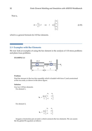
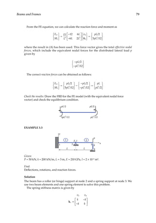
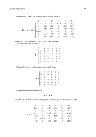
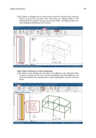
88. 73
Beams and Frames
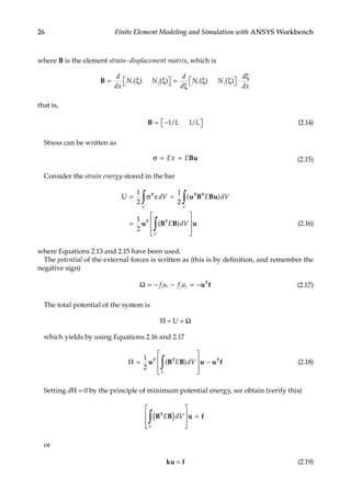
Then, on each element, we can represent the deflection of the beam (v) using shape func-
tions and the corresponding nodal values as
v x N x N x N x N x
v
v
i
i
j
j
( ) [ ( ) ( ) ( ) ( )]
= =
θ
θ














Nu 1 2 3 4 (3.7)
which is a cubic function. Note that,
N N
N N L N x
1 3
2 3 4
1
+ =
+ + =
which implies that the rigid-body motion is represented correctly by the assumed deformed
shape of the beam.
To derive the beam element stiffness matrix, we consider the curvature of the beam,
which is
d v
dx
d
dx
2
2
2
2
= =
Nu Bu (3.8)
where the strain–displacement matrix B is given by
B N
= = ′′ ′′ ′′ ′′

 

= − + − +
d
dx
N x N x N x N x
L
x
L L
x
2
2 1 2 3 4
2 3
6 12 4 6
( ) ( ) ( ) ( )
L
L L
x
L L
x
L
2 2 3 2
6 12 2 6
− − +






(3.9)
Strain energy stored in the beam element is
U = σ ε
∫
1
2
T
V
dV
Applying the basic equations in the simple beam theory, we have
U = −





 −





 =
=
∫
∫ ∫
1
2
1 1
2
1
1
2
0 0
2
My
I E
My
I
dAdx M
EI
Mdx
d v
dx
A
L T
T
L
2
2
2
2
0 0
0
1
2
1
2











 =
=
∫ ∫
T
L
T
L
T T
EI
d v
dx
dx EI dx
EI
( ) ( )
Bu Bu
u B B
L
L
dx
∫








u

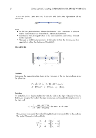
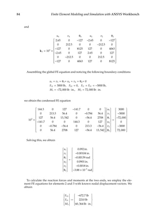
89. 74 Finite Element Modeling and Simulation with ANSYS Workbench
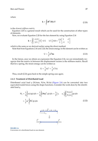
We conclude that the stiffness matrix for the simple beam element is
k B B
=
∫ T
L
EI dx
0
(3.10)
Applying the result in Equation 3.10 and carrying out the integration, we arrive at the
same stiffness matrix as given in Equation 3.5.
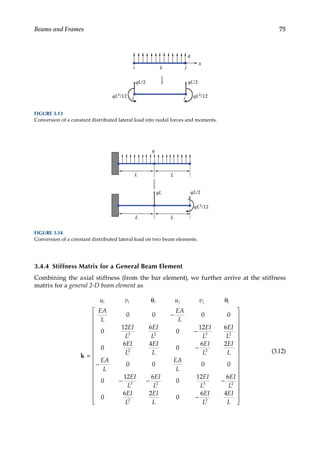
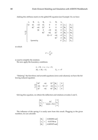
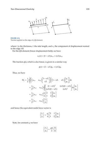
3.4.3 Treatment of Distributed Loads
To convert a distributed load into nodal forces and moments (Figure 3.12), we consider
again the work done by the distributed load q
W v x q x dx q x dx q x dx
q
L
T
L
T T
L
= = ( ) =
∫ ∫ ∫
1
2
1
2
1
2
0 0 0
( ) ( ) ( ) ( )
Nu u N
The work done by the equivalent nodal forces (and moments) is
W v v
F
M
F
M
f i i j j
i
q
i
q
j
q
j
q
T
q
q = θ θ














=
1
2
1
2
[ ] u f
By equating W W
q fq
= , we obtain the equivalent nodal force vector as
f N
q
T
L
q x dx
=
∫ ( )
0
(3.11)
which is valid for arbitrary distributions of q(x). For constant q, we have the results shown
in Figure 3.13. An example of this result is given in Figure 3.14.
x
i j
q(x)
Fi
q Fj
q
Mj
q
Mi
q
i j
L
FIGURE 3.12
Conversion of the distributed lateral load into nodal forces and moments.

90. 75
Beams and Frames
3.4.4 Stiffness Matrix for a General Beam Element
Combining the axial stiffness (from the bar element), we further arrive at the stiffness
matrix for a general 2-D beam element as
u v u v
EA
L
EA
L
EI
L
EI
L
EI
L
EI
L
EI
L
E
i i i j j j
θ θ
=
−
−
k
0 0 0 0
0
12 6
0
12 6
0
6 4
3 2 3 2
2
I
I
L
EI
L
EI
L
EA
L
EA
L
EI
L
EI
L
EI
L
EI
L
EI
L
0
6 2
0 0 0 0
0
12 6
0
12 6
0
6
2
3 2 3 2
2
−
−
− − −
2
2
0
6 4
2
EI
L
EI
L
EI
L
−


































(3.12)
x
i j
q
qL/2
i j
qL/2
L
qL2/12
qL2/12
FIGURE 3.13
Conversion of a constant distributed lateral load into nodal forces and moments.
L
q
L
L
qL
L
qL/2
qL2/12
FIGURE 3.14
Conversion of a constant distributed lateral load on two beam elements.

91. 76 Finite Element Modeling and Simulation with ANSYS Workbench
3.5 Examples with Beam Elements
EXAMPLE 3.1
E, I
M
L
P
L
y
x
2 3
1
1 2
Given:
The beam shown above is clamped at the two ends and acted upon by the force P and
moment M in the midspan.
Find:
The deflection and rotation at the center node and the reaction forces and moments at
the two ends.
Solution
Element stiffness matrices are
v v
EI
L
L L
L L L L
L L
L L L L
1 1 2 2
1 3
2 2
2 2
12 6 12 6
6 4 6 2
12 6 12 6
6 2 6 4
θ θ
=
−
−
− − −
−

k














θ θ
=
−
−
− − −
v v
EI
L
L L
L L L L
L
2 2 3 3
2 3
2 2
12 6 12 6
6 4 6 2
12 6 12
k
6
6
6 2 6 4
2 2
L
L L L L
−














Global FE equation is
v v v
EI
L
L L
L L L L
L L
L L
1 1 2 2 3 3
3
2 2
12 6 12 6 0 0
6 4 6 2 0 0
12 6 24 0 12 6
6 2
θ θ θ
−
−
− − −
2
2 2 2
2 2
0 8 6 2
0 0 12 6 12 6
0 0 6 2 6 4
L L L
L L
L L L L
−
− − −
−




















v
v
v
v
F
M
F
M
F
M
Y
Y
Y
1
1
2
2
3
3
1
1
2
2
3
3
θ
θ
θ






















=























Loads and constraints (BCs) are
F P M M v v
Y
2 2 1 3 1 3 0
= − = = = θ = θ =
, ,

92. 77
Beams and Frames
Reduced FE equation
EI
L L
v P
M
3 2
2
2
24 0
0 8





 θ







=
−







Solving this, we obtain
v L
EI
PL
M
2
2
2
24 3
θ







=
−










From the global FE equation, we obtain the reaction forces and moments
F
M
F
M
EI
L
L
L L
L
L L
Y
Y
1
1
3
3
3
2
2
12 6
6 2
12 6
6 2














=
−
−
− −















θ







=
+
+
−
− +













v
P M L
PL M
P M L
PL M
2
2
1
4
2 3
2 3
/
/


Stresses in the beam at the two ends can be calculated using the formula
σ = σ = −
x
My
I
Note that the FE solution is exact for this problem according to the simple beam
­
theory, since no distributed load is present between the nodes. Recall that
EI
d v
dx
q x
4
4
= ( )
If q(x) = 0, then exact solution for the deflection v is a cubic function of x, which is
exactly what described by the shape functions given in Equation 3.6.
EXAMPLE 3.2
1
y
2
E, I
L
p
x
Given:
A cantilever beam with distributed lateral load p as shown above.
Find:
The deflection and rotation at the right end, the reaction force and moment at the left
end.

93. 78 Finite Element Modeling and Simulation with ANSYS Workbench
Solution
The work-equivalent nodal loads are shown below,
1
y
2
E, I
L
f
m
x
where
f pL m pL
= =
/ , /
2 12
2
Applying the FE equation, we have
EI
L
L L
L L L L
L L
L L L L
3
2 2
2 2
12 6 12 6
6 4 6 2
12 6 12 6
6 2 6 4
−
−
− − −
−















θ
θ














=














v
v
F
M
F
M
Y
Y
1
1
2
2
1
1
2
2
Load and constraints (BCs) are
F f M m
v
Y
2 2
1 1 0
= − =
= θ =
,
Reduced equation is
EI
L
L
L L
v f
m
3 2
2
2
12 6
6 4
−
−





 θ







=
−







Solving this, we obtain
v L
EI
L f Lm
Lf m
pL EI
pL E
2
2
2 4
3
6
2 3
3 6
8
6
θ







=
− +
− +










=
−
−
/
/ I
I










(A)
These nodal values are the same as the exact solution. Note that the deflection v(x) (for
0 x L) in the beam by the FEM is, however, different from that by the exact solution.
The exact solution by the simple beam theory is a fourth-order polynomial of x, while
the FE solution of v is only a third-order polynomial of x.
If the equivalent moment m is ignored, we have
v L
EI
L f
Lf
pL EI
pL EI
2
2
2 4
3
6
2
3
6
4
θ







=
−
−










=
−
−






/
/





(B)
The errors in (B) will decrease if more elements are used. The equivalent moment m is
often ignored in the FEM applications. The FE solutions still converge as more elements
are applied.

94. 79
Beams and Frames
From the FE equation, we can calculate the reaction force and moment as
F
M
EI
L
L
L L
v pL
pL
Y
1
1
3 2
2
2
2
12 6
6 2
2
5 12







=
−
−





 θ







=
 /
/







where the result in (A) has been used. This force vector gives the total effective nodal
forces, which include the equivalent nodal forces for the distributed lateral load p
given by
−
−







pL
pL
/
/
2
12
2
The correct reaction forces can be obtained as follows:
F
M
pL
pL
pL
pL
pL
pL
Y
1
1
2 2 2
2
5 12
2
12







=







−
−
−







=
/
/
/
/ /2
2







Check the results: Draw the FBD for the FE model (with the equivalent nodal force
vector) and check the equilibrium condition.
pL/2
5pL2/12 pL2/12
pL/2
EXAMPLE 3.3
E, I
k
L
P
L
y
x
2 3
1
1 2
4
Given:
P = 50 kN, k = 200 kN/m, L = 3 m, E = 210 GPa, I = 2 × 10−4 m4.
Find:
Deflections, rotations, and reaction forces.
Solution
The beam has a roller (or hinge) support at node 2 and a spring support at node 3. We
use two beam elements and one spring element to solve this problem.
The spring stiffness matrix is given by
v v
k k
k k
s
3 4
k =
−
−







95. 80 Finite Element Modeling and Simulation with ANSYS Workbench
Adding this stiffness matrix to the global FE equation (see Example 3.1), we have
v v v v
EI
L
L L
L L L
L
L L L
1 1 2 2 3 3 4
3
2 2
2 2
12 6 12 6 0 0
4 6 2 0 0
24 0 12 6
8 6 2
1
θ θ θ
−
−
−
−
2
2 6
4
0
0
0
0
0
2
1
1
2
+ − −






















θ
θ
k L
L
k
Symmetry k
v
v
’ ’
’
2
2
3
3
4
1
1
2
2
3
3
4
v
v
F
M
F
M
F
M
F
Y
Y
Y
Y
θ






















=























in which
k
L
EI
k
’ =
3
is used to simplify the notation.
We now apply the boundary conditions
v v v
M M F P
Y
1 1 2 4
2 3 3
0
0
= θ = = =
= = = −
,
,
“Deleting” the first three and seventh equations (rows and columns), we have the fol-
lowing reduced equation:
EI
L
L L L
L k L
L L L
v
3
2 2
2 2
2
3
3
8 6 2
6 12 6
2 6 4
−
− + −
−










θ
θ









’


= −










0
0
P
Solving this equation, we obtain the deflection and rotations at nodes 2 and 3,
θ
θ










= −
+










2
3
3
2
12 7
3
7
9
v
PL
EI k
L
( ’)
The influence of the spring k is easily seen from this result. Plugging in the given
numbers, we can calculate
θ
θ










=
−
−
−








2
3
3
0 002492
0 01744
0 007475
v
.
.
.
rad
m
rad



96. 81
Beams and Frames
From the global FE equation, we obtain the nodal reaction forces as,
F
M
F
F
Y
Y
Y
1
1
2
4
69 78
69 78
116 2
3 488














=
−
− ⋅
.
.
.
.
kN
kN m
kN
kN















Checking the results: Draw free-body diagram of the beam
1 2
50 kN
3
3.488 kN
116.2 kN
69.78 kN
69.78 kN·m
Sum the forces and moments to verify that equilibrium of the beam is satisfied.
We use the following example to show how to model frames using the general beam
elements. This example can be used to verify the FEA results when using a software
package.
EXAMPLE 3.4
12 ft
X
1 2
3000 lb
E, I, A
Y
3
1
2 3
8 ft
500 lb/ft
4
Given: E I A
= × = =
30 10 6 8
6 2
psi, 65 in. in
4
, . .
Find:
Displacements and rotations of the two joints 1 and 2.
Solution
This is a problem of analyzing a frame. Members in a frame are considered to be rigidly
connected (e.g., welded together). Both forces and moments can be transmitted through
their joints. We need the general beam element (combinations of bar and simple beam ele-
ments) to model frames.
For this example, we first convert the distributed load into its equivalent nodal loads
to obtain the following FE mode.

97. 82 Finite Element Modeling and Simulation with ANSYS Workbench
1 2
3000 lb
3
1
2 3
3000 lb
4
3000 lb
72,000 lb-in. 72,000 lb-in.
In local coordinate system, the stiffness matrix for a general 2-D beam element is
u v u v
EA
L
EA
L
EI
L
EI
L
EI
L
EI
L
EI
L
E
i i i j j j
θ θ
=
−
−
k
0 0 0 0
0
12 6
0
12 6
0
6 4
3 2 3 2
2
I
I
L
EI
L
EI
L
EA
L
EA
L
EI
L
EI
L
EI
L
EI
L
EI
L
0
6 2
0 0 0 0
0
12 6
0
12 6
0
6
2
3 2 3 2
2
−
−
− − −
2
2
0
6 4
2
EI
L
EI
L
EI
L
−


































Element Connectivity Table
Element Node i (1) Node j (2)
1 1 2
2 3 1
3 4 2
For element 1, we have
u v u v
1 1 1 2 2 2
1 1
4
10
141 7 0 0 141 7 0 0
0 0 784 56 4 0 0 784 56
θ θ
= = ×
−
−
k k′
. .
. . . .4
4
0 56 4 5417 0 56 4 2708
141 7 0 0 141 7 0 0
0 0 784 56 4 0 0 784 56
. .
. .
. . . .
−
−
− − − 4
4
0 56 4 2708 0 56 4 5417
. .
−





















98. 83
Beams and Frames
For elements 2 and 3, the stiffness matrix in local system is
u v u v
i i i j j j
′ ′ ′ ′ ′ ′
′ ′
θ θ
= = ×
−
−
k k
2 3
4
10
212 5 0 0 212 5 0 0
0 2 65 127 0 2 6
. .
. . 5
5 127
0 127 8125 0 127 4063
212 5 0 0 212 5 0 0
0 2 65 127 0 2 65 127
0 1
−
−
− − −
. .
. .
2
27 4063 0 127 8125
−




















where i = 3, j = 1 for element 2, and i = 4, j = 2 for element 3.
The transformation matrix T is
T =
−
−


















l m
m l
l m
m l
0 0 0 0
0 0 0 0
0 0 1 0 0 0
0 0 0 0
0 0 0 0
0 0 0 0 0 1



We have l = 0, m = 1 for both elements 2 and 3. Thus,
T =
−
−


















0 1 0 0 0 0
1 0 0 0 0 0
0 0 1 0 0 0
0 0 0 0 1 0
0 0 0 1 0 0
0 0 0 0 0 1



Using the transformation relation
k T k T
= ′
T
we obtain the stiffness matrices in the global coordinate system for elements 2 and 3
u v u v
3 3 3 1 1 1
2
4
10
2 65 0 127 2 65 0 127
0 212 5 0 0 212 5 0
127 0
θ θ
= ×
− − −
−
−
k
. .
. .
8
8125 127 0 4063
2 65 0 127 2 65 0 127
0 212 5 0 0 212 5 0
127 0 4063 127 0
−
−
−
. .
. .
8
8125





















99. 84 Finite Element Modeling and Simulation with ANSYS Workbench
and
u v u v
4 4 4 2 2 2
3
4
10
2 65 0 127 2 65 0 127
0 212 5 0 0 212 5 0
127 0
θ θ
= ×
− − −
−
−
k
. .
. .
8
8125 127 0 4063
2 65 0 127 2 65 0 127
0 212 5 0 0 212 5 0
127 0 4063 127 0
−
−
−
. .
. .
8
8125




















Assembling the global FE equation and noticing the following boundary conditions
u v u v
F F F F
M
X X Y Y
3 3 3 4 4 4
1 2 1 2
1
0
3000 0 3000
72
= = θ = = = θ =
= = = = −
= −
lb lb
, , ,
,
, , , .
000 72 000
2
lb in. lb in
⋅ = ⋅
M
we obtain the condensed FE equation
10
144 3 0 127 141 7 0 0
0 213 3 56 4 0 0 784 56 4
127 56 4 13 542 0 5
4
×
−
−
−
. .
. . . .
. , 6
6 4 2708
141 7 0 0 144 3 0 127
0 0 784 56 4 0 213 3 56 4
0 56 4 2708 1
.
. .
. . . .
.
−
− − −
2
27 56 4 13 542
1
1
1
2
2
2
−




















θ
θ












. ,
u
v
u
v











=
−
−
−


















3000
3000
72 000
0
3000
72 000
,
,





Solving this, we obtain
u
v
u
v
1
1
1
2
2
2
0 092
0 00104
0 0
θ
θ






















=
−
−
.
.
.
in.
in.
0
0139
0 0901
0 0018
3 88 10 5
rad
in.
in.
rad
.
.
.
−
− ×


















−





To calculate the reaction forces and moments at the two ends, we employ the ele-
ment FE equations for elements 2 and 3 with known nodal displacement vectors. We
obtain
F
F
M
X
Y
3
3
3
672 7
2210
60 364










=
−
⋅










.
, .
lb
lb
lb in

100. 85
Beams and Frames
and
F
F
M
X
Y
4
4
4
2338
3825
112 641










=
−
⋅










lb
lb
lb in
, .
Check the results: Draw the free-body diagram of the frame as shown below. Equilibrium
is maintained with the calculated forces and moments. Recall that the problem we
solved is the one with the equivalent loads, not the one with the distributed load. Thus,
the corresponding FBD for the FE model should be applied for verifying the results.
3000 lb
3000 lb 3000 lb
72,000 lb-in.
72,000 lb-in.
2338 lb
3825 lb
112,641 lb-in.
2210 lb
60,364 lb-in.
672.7 lb
3.6 Case Study with ANSYS Workbench
Problem Description: Steel framing systems provides cost-effective solutions for low-
rise buildings. They have high strength-to-weight ratios, and can be pre-fabricated and
custom-designed. Consider the following two-story building constructed with structural
steel I-beams. Determine the deformations and the stresses in the frame when a uniform
load of 50 kN/m is applied on the second floor as shown below.
Solution
To solve the problem with ANSYS Workbench, we employ the following steps:
Step 1: Start an ANSYS Workbench Project
Launch ANSYS Workbench and save the blank project as ‘Steelframe.wbpj’.

101. 86 Finite Element Modeling and Simulation with ANSYS Workbench
Step 2: Create a Static Structural (ANSYS) Analysis System
Drag the Static Structural (ANSYS) icon from the Analysis Systems Toolbox
window and drop it inside the highlighted green rectangle in the Project
Schematic window to create a standalone static structural analysis system.
Step 3: Launch the SpaceClaim Program
Right-click on the Geometry Cell and choose Properties from its drop-down context
menu to bring up the Properties of Schematic A3: Geometry panel. From that
panel under Basic Geometric Options, select Line Bodies to enable truss model-
ing. Next, double-click on the Geometry cell to launch the SpaceClaim program.

102. 87
Beams and Frames
Step 4: Create Line Sketch
To customize units, select the SpaceClaim Options from the File menu to dis-
play the following SpaceClaim Options window. Click Units from the left
panel, and select Meters from the drop-down list of Length. Next, change the
Primary precision to 4. Also, change the Minor Grid Spacing to 1m. Click OK
to save your changes and close the window.

103. 88 Finite Element Modeling and Simulation with ANSYS Workbench
Right-click anywhere in the Graphics Window. From the drop-down context
menu, choose Select New Sketch Plane.
Mouse over x-y plane, and click to select the highlighted x-y plane. This will
change the sketch plane from the default x-z plane (shown above) to the x-y
plane (shown below).

104. 89
Beams and Frames
Click Plan View on the toolbar to view the sketch grid head-on.
Click the Sketch Mode icon on the Design tab to begin a sketch. Click on the Line
icon. To draw a line, click a start point and then an end point in the sketch grid.
When necessary, press the Esc key to end the line creation. Draw 10 lines as
shown below.

105. 90 Finite Element Modeling and Simulation with ANSYS Workbench
Step 5: Create Lines through Mirror
Click the Plane icon from the toolbar to create a plane.
Click the Home view from the toolbar. Click 3D mode to work with objects in 3D
space, and click Move from the toolbar as shown below.

106. 91
Beams and Frames
Next, click Plane from the Structure Tree on the left panel.
Click to highlight the Z-axis associated with the selected plane in the Graphics
Window, drag the Z-axis to move the selected plane backward. Type in 3 in
the distance box and press Enter. This will move the selected plane 3 meters
backward from its original location.

107. 92 Finite Element Modeling and Simulation with ANSYS Workbench
Right-click on Surface from the Structure Tree. In the drop-down context menu,
select Edit Sketch. Note: Selecting Edit Sketch will make the unwanted sur-
face disappear while keeping all the lines you just draw within the surface.
Hitting the Delete key does not work here as it will delete the surface as well
as the lines you draw.
The unwanted Surface item in the Structure Tree will be removed, as shown
below.

108. 93
Beams and Frames
Click Mirror from the toolbar, and then click Plane from the Structure Tree.
In the Graphics Window, drag to select all 10 lines as highlighted below in green.

109. 94 Finite Element Modeling and Simulation with ANSYS Workbench
The 2D frame consisting of 10 lines will be mirrored to form the two sides of a 3D
frame, as shown below.
Next, click the Remove Mirror icon from the Graphics Window to remove the
mirror plane.

110. 95
Beams and Frames
Right-click on Surface from the Structure Tree. In the drop-down context menu,
select Edit Sketch to remove the unwanted surfaces.
Next, deselect (uncheck) the Plane from the Structure Tree to hide the plane.
Click Home to display all lines in the home view.

111. 96 Finite Element Modeling and Simulation with ANSYS Workbench
Step 6: Create Lines in 3D Space
Click on the Line icon from the toolbar, and then click 3D mode to switch to 3D
sketching. To draw a line in 3D, click a start point and then an end point. Press
Esc after each line creation. Draw the 6 lines that connect the two sides of the
frame, as shown below. Right-click Surface from the Structure Tree, and select
Edit Sketch from the drop-down context menu to remove unwanted surfaces.
The following will appear afterwards, where 26 lines are included under Curves
in the Structure Tree.

112. 97
Beams and Frames
Step 7: Create a Cross Section
Click Profiles on the Prepare tab, and select the I beam icon in the New Profile
Library from the Profiles drop-down menu.
A Beam Profiles folder is now added into the Structure Tree on the left. Right-
click on I under the Beam Profiles folder, and select Edit Beam Profile from
the drop-down context menu.

113. 98 Finite Element Modeling and Simulation with ANSYS Workbench
In the Driving Dimensions folder showing up next, click on W1 to bring up its
default Ruler dimension value. Click on the default Ruler dimension value,
and change it to 0.1715m. Repeat the same steps for W2, W3, t1, t2, and t3,
and change the Ruler dimension values to 0.1715m for W2, 0.3556m for W3,
0.0073m for t1 and t2, and 0.0115m for t3. Close the SYS tab to return back to
the Graphics Window for sketch modeling.
Step 8: Assign Cross Section to Line Body
Click Select on the Design tab, and select all 26 Lines under the Curves folder in
the Structure Tree. To select all lines in the tree, click the first Line in the struc-
ture tree, and hold the Shift key and click the last Line. The selected lines will
be highlighted in yellow as shown below.

114. 99
Beams and Frames
Click Create on Prepare tab to create beams from the selected lines using the
I-beam cross-section provided. This will bring up a Beams folder in the
Structure Tree to replace the previous Curves folder. The Beams folder con-
tains 26 Beams (I-beam) as shown below.
Step 9: Move all Beams to a New Component
Click Select on the Design tab, and select all 26 Beams in the Structure Tree.
To select all beams in the tree, click the first Beam, and hold Shift key and
click the last Beam. The selected beams will be highlighted in yellow as shown
below.

115. 100 Finite Element Modeling and Simulation with ANSYS Workbench
Right-click on the highlighted Beams in the Structure Tree in the above fig-
ure, and select Move to New Component in the drop-down context menu. A
Component1 will be created in the Structure Tree with all 26 beams moved
underneath.
Next, click Component1 in the Structure Tree, and change the Share Topology to
Merge in the bottom left Properties menu to merge all the beams.

116. 101
Beams and Frames
Click Display on the Prepare tab, and click Solid Beams to show beam profiles
and orientations.
Note that 8 beams are used as H-beams in the above configuration. To fix the
misaligned cross sections, click Orient on the Prepare tab, and Ctrl-click the 8
beams labeled below to select them from the Graphics Window. Alternatively,
you may also Ctrl-click the 8 beams underneath Component1 to select them
from the left Structure Tree. In the lower left Properties panel, enter 90 for
Orientation to turn the H-beams 90 degrees about their neutral axes.

117. 102 Finite Element Modeling and Simulation with ANSYS Workbench
The adjusted frame shown below now has all the I-beams oriented in the strong-
axis configuration. This completes the geometry creation of a frame structure.
Save and exit SpaceClaim.
Step 10: Launch the Static Structural (ANSYS) Program
Double-click the Model cell to launch the Static Structural program. Note that in
the Details of “Beam1” the material is assigned to Structural Steel by default.

118. 103
Beams and Frames
Step 11: Generate Mesh
In the Details of “Mesh”, enter ‘0.2’ for the Element Size. In the Outline of
Project, right-click on Mesh and select Generate Mesh.
After completion, the meshed structure appears. You may deselect the Ruler
from the View drop-down menu to turn off the ruler display in the Graphics
Window.

119. 104 Finite Element Modeling and Simulation with ANSYS Workbench
Step 12: Apply Boundary Conditions
In the Outline of Project, right-click on Static Structural (A5) and select Insert
and then Fixed Support. After completion, a Fixed Support item is added
underneath Static Structural (A5) in the project outline tree.
Select the six points as shown below in the Graphics Window. In the Details
of “Fixed Support”, click Apply to confirm on the Geometry selection. After
completion, a Fixed Support boundary condition will be added to the selected
six points.

120. 105
Beams and Frames
Step 13: Apply Loads
In the Outline of Project, right-click on Static Structural (A5) and select Insert
and then Line Pressure.
Ctrl-click the 7 line shown below in red in the Graphics Window. In the Details
of “Line Pressure”, click Apply to confirm on the Geometry selection. Also,
change the Define By selection to Components and enter ‘-50000’ for the Y
Component. A downward red arrow will appear on the selected line in the
Graphics Window.

121. 106 Finite Element Modeling and Simulation with ANSYS Workbench
Alternative Procedure: Note that the Line Pressure item in the Outline tree can
be copied and pasted under Static Structural (A5) for repeated use. To make
a copy, right-click on a Line Pressure item and select Copy from the menu. To
paste, right-click on the Static Structural (A5) and select Paste. Remember
to apply each newly pasted Line Pressure item to a different line edge on the
Geometry selection in the Details of “Line Pressure” until the same load is
applied to all seven edges.
Step 14: Retrieve Solution
Insert a Total Deformation item by right-clicking on Solution (A6) in the Outline
tree.
Insert a Beam Tool item by right-clicking on Solution (A6) in the Outline tree.

122. 107
Beams and Frames
Right-click on Solution (A6) in the Outline tree and select Solve. The program
will start to solve the model.
After completion, click Total Deformation in the Outline to review the total
deformation results.

123. 108 Finite Element Modeling and Simulation with ANSYS Workbench
Click Direct Stress under Beam Tool in the Outline to review the axial stress
results in beams.
Click Minimum Combined Stress under Beam Tool to retrieve the linear combi-
nation of the Direct Stress and the Minimum Bending Stress results in beams.

124. 109
Beams and Frames
Click Maximum Combined Stress under Beam Tool to retrieve the linear combi-
nation of the Direct Stress and the Maximum Bending Stress results in beams.
Close the Static Structural program. Save the project and exit ANSYS Workbench.
Modeling tips: To add a deck structure to the building frame, a surface body can
be created using the existing geometry features as follows. First, double-click
the Geometry cell in the Project Schematic to start SpaceClaim, and click
Select on the Design tab of the SpaceClaim program. Next, Ctrl-click the four
beams highlighted in the figure below, and click the Blend icon from the tool-
bar. Set the Appearance Layout to True in the lower left Properties panel. Click
the Check Mark icon in the Graphics Window to complete the surface creation.

125. 110 Finite Element Modeling and Simulation with ANSYS Workbench
Click Surface under Component1 in the Structure Tree, enter 0.05 for Midsurface
Thickness in the lower left Properties panel. A surface body with thickness of
0.05 meters is now created.
Exit SpaceClaim, and start the Static Structural program. Right-click on Mesh in
the Project Outline Tree, and click Generate Mesh. The following mesh will
be generated on model.

126. 111
Beams and Frames
Reassign the line pressure to the 7 edges as shown below. Also make sure that the
Fixed Support condition is added to the bottom 6 points of the frame.
Right-click on Solution from the Project Outline Tree, and click Solve. After
completion, click Total Deformation in the Outline to review the total defor-
mation results. Compare the new set of results with the previous results
achieved without considering a surface deck. There is about 12.5% reduction
in the maximum total deformation by including a 0.05m surface deck in the
model.

127. 112 Finite Element Modeling and Simulation with ANSYS Workbench
3.7 Summary
This chapter is devoted to the beam element and frame analysis. We have studied the
beam element, which can be used in frame analysis. The concept of the shape functions is
further explored and the derivations of the stiffness matrix using the energy approach are
emphasized. Treatment of distributed loads is discussed and several examples are stud-
ied. A two-story building structure with I-beams is analyzed using ANSYS Workbench.
It provides useful modeling techniques in constructing concept line models, and shows
step-by-step how Workbench can be used to determine the deformation and stresses in
beams and frames.
3.8 Review of Learning Objectives
Now that you have finished this chapter, you should be able to
1. Set up simplified finite element models for beams and frames.
2. Derive the element stiffness matrix for plane beams using direct/energy approach.
3. Explain the concept of shape functions and their characteristics for beam elements.
4. Find the equivalent nodal forces of distributed loads on beams.
5. Determine the deflection and rotation at a point of a beam using hand calculation
to verify the finite element solutions.
6. Apply the general beam element stiffness matrix to the analysis of simple frames.
7. Create line models from concept points, sketches, or by body translation in
Workbench.
8. Perform static structural analyses on beams and frames using Workbench.
PROBLEMS
3.1 Using Equation 3.11, derive the results of the equivalent nodal forces and
moments for a beam element with uniformly distributed lateral load.
3.2 The cantilever beam is supported by a spring at the end as shown in the figure.
Using FEM, determine the deflection and rotation at the node 2.
E, I
k
P
L
y
x
1
3
2

128. 113
Beams and Frames
3.3 Using FEM, determine the nodal displacement, rotations, and reaction forces
for the propped cantilever beam shown below. The beam is assumed to have
constant EI and length 2L. It is supported by a roller at mid length and is built
in at the right end.
P
L
X
1 2
E, I
Y
L
3
1 2
3.4 The 2-D frame is supported as shown in the figure. Constants E, A, I of the beam
and the length L are given. Using FEM, determine the displacement and rota-
tion at node 2.
L X
1 2
M
Y
3
L
3.5 The plane frame is subjected to the uniformly distributed load and is fixed
at the ends as shown in the figure. Assume E = 30 × 106 psi, A = 100 in.2, and
I = 1000 in.4 for both elements of the frame. Using FEM, find the displacement
and rotation of node 2.
40 ft
X
1
1000 lb/ft
Y
30 ft
45°
3
2
3.6 Using ANSYS Workbench, solve the frame problem in Problem 3.5, and deter-
mine the reaction forces and moments at the two fixed ends.

129. 114 Finite Element Modeling and Simulation with ANSYS Workbench
3.7 The physical construction of two representative beam connections is shown in
the figure below, where an I-beam is connected to a floor slab through a slotted
bolt hole in (a), and is connected to a column through an angle bracket in (b).
What simplified support conditions would you use to represent the physical
construction in the two cases and explain your reasons?
(b)
(a)
3.8 The bike frame shown in the figure below has hollow circular tubes (24 mm
outer diameter and 2 mm thick) and is made of aluminum alloy. Use ANSYS
Workbench to determine the deformation and stresses of the frame members.
(mm)
coordinate
Point
z
y
x
1 0
400
400
2 –150 0
350
3 0
300
450
4 0
0
0
5 600
600
50
50
6 50 –50
7 –450 50 50
8 –450 50 –50
3
2
4
5
6
7
8
540 N
180 N
80 N
1
3.9 The hoist frame shown in the following figure has 76 mm wide and 3 mm thick
square tubes and is made of structural steel. Use ANSYS Workbench to deter-
mine the deformation and the stresses in the frame.
8000 N
1 2 3
4
5 6 7
8 9
10
11
12
13
14
15
16
17
0.5 m 0.5 m
2 m
1.6 m
0.3 m
1 m
0.2 m
1.2 m
0.2 m

130. 115
Beams and Frames
3.10 The frame structure is constructed with structural steel I-beams of given cross-
section dimensions and is used to support a uniform load of 6 kN/m as shown
below. Use ANSYS Workbench to determine the deformation and stresses in the
frame members.
6 kN/m
6 kN/m 0.3 m
0.3 m
1.2 m
0.5 m
80 mm
5 mm
25 mm 5 mm
3.11 The following bridge structure is used to carry a uniform load of 50 kN/m on
the bridge surface. Use ANSYS Workbench to determine the deformation and
stresses in the bridge if structural steel I-beams of the given cross-section are
used.
1 m 1.5 m 1.5 m 1 m
2 m
1 m
0.2 m
0.2 m
50 kN/m
0.2 m
0.28 in.
4.06 in.
4.16 in.
0.375 in.

132. 117
4
Two-Dimensional Elasticity
4.1 Introduction
Many structures that are three-dimensional can be satisfactorily treated as two-dimen-
sional problems (Figure 4.1). This chapter introduces you to the use of the finite element
method for deformation and stress analyses of two-dimensional elasticity problems. First,
the basic equations in plane elasticity theory are reviewed. Then several types of 2-D finite
elements for plane elasticity analysis are presented. Applications of these elements are
demonstrated and their accuracies and efficiencies are discussed. This presentation is
followed by an example illustrating analysis of a 2-D elasticity problem using ANSYS®
Workbench.
4.2 Review of 2-D Elasticity Theory
In general, the stresses and strains at any point in a structure consist of six independent
components, that is (Figure 4.2),
σ σ σ τ τ τ
x y z xy yz zx
, , , , ,
for stresses, and
ε ε ε γ γ γ
x y z xy yz zx
, , , , ,
for strains.
Under certain conditions, the state of stresses and strains can be simplified. A 3-D stress
analysis can, therefore, be reduced to a 2-D analysis. There are two general types of models
involved in this 2-D analysis: plane stress and plane strain.
4.2.1 Plane Stress
In the plane stress case, any stress component related to the z direction is zero, that is,
σ = τ = τ = ε ≠
z yz zx z
0 0
( ) (4.1)

133. 118 Finite Element Modeling and Simulation with ANSYS Workbench
A thin planar structure with constant thickness and loading within the plane of the
structure (xy-plane) can be regarded as a plane stress case (Figure 4.3).
4.2.2 Plane Strain
In the plane strain case, any strain component related to the z direction is zero, that is,
ε = γ = γ = σ ≠
z yz zx z
0 0
( ) (4.2)
A long structure with a uniform cross section and transverse loading along its thickness
(z-direction), such as a tunnel or a dam, can be regarded a plane strain case (Figure 4.4).
As illustrated in the above figures, structures in plane stress or plane strain condi-
tions can be modeled as 2-D boundary value problems. At an arbitrary point, the in-
plane ­
displacement field may be defined by two components (u and v), the in-plane strain
field by three components (ε ε γ
x y xy
, , ), and the in-plane stress field by three components
(σ σ τ
x y xy
, , ). The following is a review of equations describing how the field variables are
related.
x
z
y
σy
σz
σx
τzx
τxy
τyz
FIGURE 4.2
Stress components at a point in a structure.
A rotating disk A reservoir dam
River
(b)
(a)
FIGURE 4.1
Examples of 2-D elasticity problems.

134. 119
Two-Dimensional Elasticity
4.2.3 Stress–Strain (Constitutive) Equations
For linear elastic isotropic materials, we have the following strain–stress relation for the
plane stress case:
ε
ε
γ










=
−ν
−ν










σ
σ
τ


x
y
xy
x
y
xy
E E
E E
G
1 0
1 0
0 0 1
/ /
/ /
/









+
ε
ε
γ










x
y
xy
0
0
0
(4.3)
or,
ε = σ + ε
−
E 1
0
where ε0 is the initial strain (e.g., due to a temperature change), E Young’s modulus, ν
Poisson’s ratio, and G the shear modulus. Note that
G
E
=
+
2 1
( )
ν
(4.4)
for homogeneous and isotropic materials.
x
y
z
(a) (b)
y
x
FIGURE 4.3
Plane stress condition: (a) structure with in-plane loading; and (b) 2-D model.
x
y
z x
y
(a) (b)
FIGURE 4.4
Plane strain condition: (a) structure with uniform transverse load; and (b) 2-D model.

135. 120 Finite Element Modeling and Simulation with ANSYS Workbench
We can also express stresses in terms of strains by solving the above equation
σ
σ
τ










=
− ν
ν
ν
− ν










ε
ε
γ



x
y
xy
x
y
xy
E
1
1 0
1 0
0 0 1 2
2
( )/ 







−
ε
ε
γ




















x
y
xy
0
0
0
(4.5)
or,
σ = ε + σ
E 0
where σ = − ε
0 0
E is the initial stress.
For plane strain case, we need to replace the material constants in the above equations in
the following fashion:
E
E
G G
→
−
→
−
→
1 1
2
ν
ν
ν
ν
; ; (4.6)
For example, the stress is related to strain by
σ
σ
τ










=
+ ν − ν
− ν
−
− ν








x
y
xy
E
( )( )
( )
1 1 2
1 0
1 0
0 0 1 2 2
ν
ν ν
/



ε
ε










−
ε
ε
γ




















x
y
xy
x
y
xy
γ
0
0
0
in the plane strain case.
Initial strain due to a temperature change (thermal loading) is given by the following for
the plane stress case
ε
ε
γ










=
α
α










x
y
xy
T
T
0
0
0 0
∆
∆ (4.7)
where α is the coefficient of thermal expansion, ΔT the change of temperature. For the
plane strain case, α should be replaced by (1 + ν)α in Equation 4.7. Note that if the struc-
ture is free to deform under thermal loading, there will be no (elastic) stresses in the
structure.
4.2.4 Strain and Displacement Relations
For small strains and small rotations, we have,
ε =
∂
∂
ε =
∂
∂
γ =
∂
∂
+
∂
∂
x y xy
u
x
v
y
u
y
v
x
, ,

136. 121
Two-Dimensional Elasticity
In matrix form, we write
ε
ε
γ










=
∂ ∂
∂ ∂
∂ ∂ ∂ ∂
















ε
x
y
xy
x
y
y x
u
v
/
/
/ /
or
0
0 , =
= Du (4.8)
From this relation, we know that, if the displacements are represented by polynomials,
the strains (and thus stresses) will be polynomials of an order that is one order lower than
the displacements.
4.2.5 Equilibrium Equations
In plane elasticity, the stresses in the structure must satisfy the following equilibrium
equations:
∂σ
∂
+
∂τ
∂
+ =
∂τ
∂
+
∂σ
∂
+ =
x xy
x
xy y
y
x y
f
x y
f
0
0
(4.9)
where fx and fy are body forces (forces per unit volume, such as gravity forces). In the FEM,
these equilibrium conditions are satisfied in an approximate sense.
4.2.6 Boundary Conditions
The boundary S of the 2-D region can be divided into two parts, Su and St (Figure 4.5). The
boundary conditions (BCs) can be described as
u u v v S
t t t t S
u
x x y y t
= =
= =
, ,
, ,
on
on
(4.10)
in which tx and ty are tractions (stresses on the boundary) and the barred quantities are
those with known values.
4.2.7 Exact Elasticity Solution
The exact solution (displacements, strains, and stresses) of a given problem must satisfy
the constitutive relations, equilibrium equations, and compatibility conditions (structures
x
y
p
tx
ty
Su
St
FIGURE 4.5
Boundary conditions for a structure.

137. 122 Finite Element Modeling and Simulation with ANSYS Workbench
should deform in a continuous manner, with no cracks or overlaps in the obtained dis-
placement fields).
EXAMPLE 4.1
x
y p
A plate is supported and loaded with distributed force p as shown in the figure. The
material constants E and ν are known.
The exact solution for this simple problem is found to be as follows:
Displacement:
u
p
E
x v
p
E
y
= = −ν
,
Strain:
εx y xy
p
E
p
E
= = −ν =
, ,
ε γ 0
Stress:
σ = σ = τ =
x y xy
p, ,
0 0
Exact (or analytical) solutions for simple problems are numbered (suppose there is a
hole in the plate or the roller supports are replaced by fixed ones). That is why we need
the FEM for solutions of 2-D elasticity problems in general.
4.3 Modeling of 2-D Elasticity Problems
For a plane stress or plane strain analysis, we model only a 2-D region, that is, a planar
surface or cross section of the original 3-D structure. The region then needs to be divided
into an element discretization made of triangles, quadrilaterals, or a mixture of both. The
element behaviors need to be specified to set up the problem type as either plane stress
or plane strain. The discretization can be structured (mapped mesh on a three-sided or
four-sided surface region with equal numbers of element divisions for the opposite sides)
or unstructured (free mesh), as shown in Figure 4.6. A structured surface mesh has ­
regular

138. 123
Two-Dimensional Elasticity
connectivity that can be described as a 2-D array, and it generally has better solution reli-
ability compared to a free mesh.
Mesh properties such as the mesh density and the element shape quality are important
factors that affect the solution accuracy and efficiency. Finer mesh is usually needed in
areas where a high stress/strain is expected. The type of finite element employed also
plays a vital role in the analysis, as will be discussed in the next section.
After meshing is complete, the surface discretization is represented in terms of nodal
coordinates as well as element connectivity showing how different elements are connected
together through nodes. All types of loads (distributed forces, concentrated forces and
moments, and so on) are converted into point forces acting at individual nodes. Boundary
conditions are no exception, and will be converted into nodal DOF constraints. Remember
that support conditions need to suppress rigid-body motion, and the minimum conditions
in 2-D include restraining the body with displacement in x, y directions and rotation about
the z-axis. Figure 4.7 gives examples of effective and ineffective support conditions in 2-D.
Explain why a case is effective or not.
4.4 Formulation of the Plane Stress/Strain Element
In this section, we formulate the element equations based on the plane elasticity theory. A
general formula for the stiffness matrix is derived first, followed by presentation of several
common element types for 2-D elasticity problems.
(a) (b)
FIGURE 4.6
Finite element discretization: (a) unstructured (free) mesh; and (b) structured (mapped) mesh.
(b) (c)
(a)
FIGURE 4.7
Support conditions in 2-D: (a) and (c) effective constraints; (b) ineffective constraints.

139. 124 Finite Element Modeling and Simulation with ANSYS Workbench
4.4.1 A General Formula for the Stiffness Matrix
Displacements (u, v) in a plane element can be interpolated from nodal displacements
(ui, vi) using shape functions Ni as follows:
u
v
N N
N N
u
v
u
v






=
























1 2
1 2
1
1
2
2
0 0
0 0
or u
u Nd
= (4.11)
where N is the shape function matrix, u the displacement vector, and d the nodal displace-
ment vector. Here, we have assumed that u depends on the nodal values of u only, and v
on nodal values of v only.
From strain–displacement relation (Equation 4.8), the strain vector is
ε = = ε =
Du DNd Bd
, or (4.12)
where B = DN is the strain–displacement matrix.
Consider the strain energy stored in an element,
U = σ ε = σ ε + σ ε + τ γ
( )
= ε
( ) ε = ε ε
∫ ∫
∫
1
2
1
2
1
2
1
2
T
V
x x y y xy xy
V
T
V
T
dV dV
dV dV
E E
V
V
T T
V
T
dV
∫ ∫
=
=
1
2
1
2
d B EB d
d kd
From this, we obtain the general formula for the element stiffness matrix
k B EB
=
∫ T
V
dV (4.13)
Note that unlike the 1-D cases, E here is a matrix which is given by the stress–strain rela-
tion (e.g., Equation 4.5 for plane stress).
The stiffness matrix k defined by Equation 4.13 is symmetric since E is symmetric. Also
note that given the material property, the behavior of k depends on the B matrix only, which
in turn depends on the shape functions. Thus, the quality of finite elements in representing
the behavior of a structure is mainly determined by the choice of shape functions. Most
commonly employed 2-D elements are linear or quadratic triangles and quadrilaterals.
4.4.2 Constant Strain Triangle (CST or T3)
This is the simplest 2-D element (Figure 4.8), which is also called linear triangular element.
For this element, we have three nodes at the vertices of the triangle, which are numbered
around the element in the counterclockwise direction. Each node has two DOFs (can move

140. 125
Two-Dimensional Elasticity
in the x and y directions). The displacements u and v are assumed to be linear functions
within the element, that is
u b b x b y v b b x b y
= + + = + +
1 2 3 4 5 6
, (4.14)
where bi (i = 1, 2, …, 6) are constants. From these, the strains are found to be
ε = ε = γ = +
x y xy
b b b b
2 6 3 5
, , (4.15)
which are constant throughout the element. Thus, we have the name “constant strain tri-
angle” (CST).
Displacements given by Equation 4.14 should satisfy the following six equations:
u b b x b y
u b b x b y
v b b x b y
1 1 2 1 3 1
2 1 2 2 3 2
3 4 5 3 6 3
= + +
= + +
= + +
Solving these equations, we can find the coefficients b1, b2, …, and b6 in terms of nodal
displacements and coordinates. Substituting these coefficients into Equation 4.14 and rear-
ranging the terms, we obtain
u
v
N N N
N N N
u
v
u
v
u
v






=



















1 2 3
1 2 3
1
1
2
2
3
3
0 0 0
0 0 0










(4.16)
x
y
1
3
2
(x1, y1)
(x2, y2)
(x3, y3)
u
v
(x, y)
u1
v1
v2
u2
u3
v3
FIGURE 4.8
Linear triangular element (T3).

141. 126 Finite Element Modeling and Simulation with ANSYS Workbench
where the shape functions (linear functions in x and y) are
N
A
x y x y y y x x x y
N
A
x y x y y
1 2 3 3 2 2 3 3 2
2 3 1 1 3 3
1
2
1
2
= − + − + −
{ }
= − +
( ) ( ) ( )
( ) ( −
− + −
{ }
= − + − + −
{ }
y x x x y
N
A
x y x y y y x x x y
1 1 3
3 1 2 2 1 1 2 2 1
1
2
) ( )
( ) ( ) ( )
(4.17)
and
A
x y
x y
x y
=










1
2
1
1
1
1 1
2 2
3 3
det (4.18)
is the area of the triangle.
Using the strain–displacement relation (4.8), results (4.16) and (4.17), we have
ε
ε
γ










= =
x
y
xy
A
y y y
x x x
x y x y
Bd
1
2
0 0 0
0 0 0
23 31 12
32 13 21
32 23 13 3
31 21 12
1
1
2
2
3
3
x y
u
v
u
v
u
v
































(4.19)
where xij = xi − xj and yij = yi − yj (i, j = 1, 2, 3). Again, we see constant strains within the ele-
ment. From stress–strain relation (e.g., Equation 4.5), we see that stresses obtained using
the CST element are also constant.
Applying the formula in Equation 4.13, we obtain the element stiffness matrix for the
CST element
k B EB B EB
= =
∫ T
V
T
dV tA( ) (4.20)
in which t is the thickness of the element. Notice that k for CST is a 6 × 6 symmetric matrix.
Both the expressions of the shape functions in Equation 4.17 and their derivations are
lengthy and offer little insight into the behavior of the element.
We introduce the natural coordinates (ξ, η) on the triangle where ξ = η =
A A A A
1 2
/ /
, with
A1 and A2 being the areas of the smaller triangles indicated in Figure 4.9. Then the shape
functions can be represented simply by
N N N
1 2 3 1
= ξ = η = − ξ − η
, , (4.21)
Notice that,
N N N
1 2 3 1
+ + = (4.22)

142. 127
Two-Dimensional Elasticity
which ensures that the rigid-body translation is represented by the chosen shape func-
tions. Also, as in the 1-D case,
N
i
i =



1
0
,
,
atnode ;
at other nodes
(4.23)
and varies linearly within the element. The plot for shape function N1 is shown in Figure
4.10. N2 and N3 have similar features.
We have two coordinate systems for the element: the global coordinates (x, y) and the
natural (local) coordinates (ξ, η). The relation between the two is given by
x N x N x N x
y N y N y N y
= + +
= + +
1 1 2 2 3 3
1 1 2 2 3 3
(4.24)
or,
x x x x
y y y y
= ξ + η +
= ξ + η +
13 23 3
13 23 3
(4.25)
where xij = xi − xj and yij = yi − yj (i, j = 1, 2, 3) as defined earlier.
1
3
2
ξ = 0
ξ = 1
ξ = a
η = 0
η = b
η = 1
(a, b)
A1
A2
FIGURE 4.9
The natural coordinate system defined on the triangle.
1
3
2
ξ = 0
ξ = 1
N1
1
FIGURE 4.10
Plot of the shape function N1 for T3 element.

143. 128 Finite Element Modeling and Simulation with ANSYS Workbench
Displacement u or v on the element can be viewed as functions of (x, y) or (ξ, η). Using the
chain rule for derivatives, we have
∂
∂ξ
∂
∂η














=
∂
∂ξ
∂
∂ξ
∂
∂η
∂
∂η












∂
∂
∂
∂
u
u
x y
x y
u
x
u
y
y
u
x
u
y














=
∂
∂
∂
∂














J (4.26)
where J is called the Jacobian matrix of the transformation.
From Equation 4.25, we calculate
J J
=





 =
−
−






−
x y
x y A
y y
x x
13 13
23 23
1 23 13
23 13
1
2
, (4.27)
where det J = − =
x y x y A
13 23 23 13 2 has been used (A is the area of the triangle).
From Equations 4.26, 4.27, 4.16, and 4.21, we have
∂
∂
∂
∂














=
−
−






∂
∂ξ
∂
∂η




u
x
u
y
A
y y
x x
u
u
1
2
23 13
23 13











=
−
−






−
−






1
2
23 13
23 13
1 3
2 3
A
y y
x x
u u
u u
(4.28)
Similarly,
∂
∂
∂
∂














=
−
−






−
−


v
x
v
y
A
y y
x x
v v
v v
1
2
23 13
23 13
1 3
2 3





(4.29)
Using the results in Equations 4.28 and 4.29, and the relations ε = = =
Du DNd Bd, we
obtain the strain–displacement matrix,
B =










1
2
0 0 0
0 0 0
23 31 12
32 13 21
32 23 13 31 21 12
A
y y y
x x x
x y x y x y
(4.30)
which is the same as we derived earlier in Equation 4.19.
We should note the following about the CST element:
• Use in areas where the strain gradient is small.
• Use in mesh transition areas (fine mesh to coarse mesh).
• Avoid using CST in stress concentration or other crucial areas in the structure,
such as edges of holes and corners.
• Recommended only for quick and preliminary FE analysis of 2-D problems.

144. 129
Two-Dimensional Elasticity
4.4.3 Quadratic Triangular Element (LST or T6)
This type of element (Figure 4.11) is also called quadratic triangular element. There are six
nodes on this element: three corner nodes and three midside nodes. Each node has two
DOFs as before. The displacements (u, v) are assumed to be quadratic functions of (x, y),
u b b x b y b x b xy b y
v b b x b y b x b xy b y
= + + + + +
= + + + + +
1 2 3 4
2
5 6
2
7 8 9 10
2
11 12
2
(4.31)
where bi (i = 1, 2, …, 12) are constants. From these, the strains are found to be
ε = + +
ε = + +
γ = + + + + +
x
y
xy
b b x b y
b b x b y
b b b b x b
2 4 5
9 11 12
3 8 5 10 6
2
2
2 2
( ) ( ) ( b
b y
11)
(4.32)
which are linear functions. Thus, we have the “linear strain triangle” (LST), which pro-
vides better results than the CST.
In the natural coordinate system, the six shape functions for the LST element are
N
N
N
N
N
N
1
2
3
4
5
6
2 1
2 1
2 1
4
4
4
= ξ ξ −
= η η −
= ζ ζ −
= ξη
= ηζ
= ζξ
( )
( )
( )
(4.33)
in which ζ = 1 − ξ − η. Each of these six shape functions represents a quadratic form on the
element as shown in Figure 4.12.
x
y
1
3
2
u1
v1
u2
v2
u3
v3
u4
v4
u5
v5
u6
v6
6
5
4
FIGURE 4.11
Quadratic triangular element (T6).

145. 130 Finite Element Modeling and Simulation with ANSYS Workbench
Displacements can be written as
u N u v N v
i i
i
i i
i
= =
= =
∑ ∑
1
6
1
6
, (4.34)
The element stiffness matrix is still given by k B EB
= ∫V
T
dV, but here BTEB is quadratic
in x and y. In general, the integral has to be computed numerically.
4.4.4 Linear Quadrilateral Element (Q4)
There are four nodes at the corners of the quadrilateral element (Figure 4.13). In the natural
coordinate system (ξ, η), the four shape functions are
N
N
N
N
1
2
3
4
1
4
1 1
1
4
1 1
1
4
1 1
1
4
1 1
= − ξ − η
= + ξ − η
= + ξ + η
= − ξ +
( )( )
( )( )
( )( )
( )( η
η)
(4.35)
1
3
2
ξ = 0
ξ = 1 N1
1
ξ = 1/2
6 5
4
FIGURE 4.12
Plot of the shape function N1 for T6 element.
x
y
1
3
2
u4
v4
u1
v1
u2
v2
u3
v3
4
η = 1
η = –1
ξ = –1 ξ = 1
ξ
η
FIGURE 4.13
Linear quadrilateral element (Q4).

146. 131
Two-Dimensional Elasticity
Note that ∑ =
=
i i
N
1
4
1 at any point inside the element, as expected.
The displacement field is given by
u N u v N v
i i
i
i i
i
= =
= =
∑ ∑
1
4
1
4
, (4.36)
which are bilinear functions over the element. The stress and strain fields are constant on
this type of elements.
4.4.5 Quadratic Quadrilateral Element (Q8)
This is the most widely used element for 2-D problems due to its high accuracy in analysis
and flexibility in modeling.
There are eight nodes for this element (Figure 4.14), four corners nodes and four midside
nodes. In the natural coordinate system (ξ, η), the eight shape functions are
N
N
N
1
2
3
1
4
1 1 1
1
4
1 1 1
1
4
1 1
= − ξ η − ξ + η +
= + ξ η − η − ξ +
= + ξ + η
( )( )( )
( )( )( )
( )( )
)( )
( )( )( )
( )( )
( )(
ξ + η −
= ξ − η + ξ − η +
= − η − ξ
= + ξ
1
1
4
1 1 1
1
2
1 1
1
2
1
4
5
2
6
N
N
N 1
1
1
2
1 1
1
2
1 1
2
7
2
8
2
− η
= + η − ξ
= − ξ − η
)
( )( )
( )( )
N
N
(4.37)
x
y
1
3
2
4
6
7
5
8
η = 1
η = –1
ξ = –1 ξ = 1
ξ
η
FIGURE 4.14
Quadratic quadrilateral element (Q8).

147. 132 Finite Element Modeling and Simulation with ANSYS Workbench
Again, we have ∑ =
=
i i
N
1
8
1 at any point inside the element.
The displacement field is given by
u N u v N v
i i
i
i i
i
= =
= =
∑ ∑
1
8
1
8
, (4.38)
which are quadratic functions over the element. Strains and stresses over a quadratic
quadrilateral element are linear functions, which are better representations. A model of
fiber-reinforced composite materials using the Q8 elements is shown in Figure 4.15.
We need to note the following when applying the 2-D elements:
• Q4 and T3 are usually used together in a mesh with linear elements.
• Q8 and T6 are usually applied in a mesh composed of quadratic elements.
• Linear elements are good for deformation analysis, that is, when global responses
need to be determined.
• Quadratic elements are preferred for stress analysis, because of their high accu-
racy and the flexibility in modeling complex geometry, such as curved boundaries.
4.4.6 Transformation of Loads
Concentrated load (point forces), surface traction (pressure loads), and body force (weight)
are the main types of loads applied to a structure. Both traction and body forces need to be
converted into nodal forces in the FE model, since they cannot be applied to the FE model
directly. The conversions of these loads are based on the same idea (the equivalent-work
concept), which we have used for the cases of bar and beam elements.
Suppose, for example, we have a linearly varying traction q on a Q4 element edge, as
shown in the Figure 4.16. The traction is normal to the boundary. Using the local (tangen-
tial) coordinate s, we can write the work done by the traction q as
W t u s q s ds
q n
L
=
∫
1
2
0
( ) ( )
FIGURE 4.15
Analysis of composite materials (mesh and contour stress plots).

148. 133
Two-Dimensional Elasticity
where t is the thickness, L the side length, and un the component of displacement normal
to the edge AB.
For the Q4 element (linear displacement field), we have
u s s L u s L u
n nA nB
( ) ( ) ( )
= − +
1 / /
The traction q(s), which is also linear, is given in a similar way
q s s L q s L q
A B
( ) ( ) ( )
= − +
1 / /
Thus, we have
W t u u
s L
s L
s L s L
q
q
q nA nB
A
B
= 
 

−











 −

 







1
2
1
1
/
/
/ /







= 
 

− −
−
∫ ds
u u t
s L s L s L
s L s L
L
nA nB
0
2
1
2
1 1
1
( ) ( )( )
( )( )
/ / /
/ / (
( )
s L
ds
q
q
u u
tL q
q
L
A
B
nA nB
A
B
/ 2
0
1
2 6
2 1
1 2












= 
 







∫







= 
 







1
2
u u
f
f
nA nB
A
B
and hence the equivalent nodal force vector is
f
f
tL q
q
A
B
A
B






=












6
2 1
1 2
Note, for constant q, we have
f
f
qtL
A
B






=






2
1
1
A
B
L
s
q
qA
qB
A
B
fA
fB
FIGURE 4.16
Traction applied on the edge of a Q4 element.

149. 134 Finite Element Modeling and Simulation with ANSYS Workbench
For quadratic elements (either triangular or quadrilateral), the traction is converted into
forces at three nodes along the edge, instead of two nodes. Traction tangent to the bound-
ary, as well as body forces, are converted into nodal forces in a similar way.
4.4.7 Stress Calculation
The stress in an element is determined by the following relation:
σ
σ
τ










=
ε
ε
γ










=
x
y
xy
x
y
xy
E EBd (4.39)
where B is the strain-nodal displacement matrix and d is the nodal displacement vector,
which is known for each element once the global FE equation has been solved.
Stresses can be evaluated at any point inside the element (such as the center) or at the
nodes. Contour plots are usually used in FEA software packages (during postprocess) for
users to visually inspect the stress results.
4.4.7.1 The von Mises Stress
The von Mises stress is the effective or equivalent stress for 2-D and 3-D stress analysis. For
a ductile material, the stress level is considered to be safe, if
σ ≤ σ
e Y
where σe is the von Mises stress and σY the yield stress of the material. This is a generaliza-
tion of the 1-D (experimental) result to 2-D and 3-D situations.
The von Mises stress is defined by
σ = σ − σ + σ − σ + σ − σ
e
1
2
1 2
2
2 3
2
3 1
2
( ) ( ) ( ) (4.40)
in which σ1, σ2 and σ3 are the three principle stresses at the considered point in a structure.
For 2-D problems, the two principle stresses in the plane are determined by
σ =
σ + σ
+
σ − σ





 + τ
σ =
σ + σ
−
σ − σ





 + τ
1
2
2
2
2
2
2 2
2 2
P x y x y
xy
P x y x y
xy
(4.41)
Thus, we can also express the von Mises stress in terms of the stress components in the
xy coordinate system. For plane stress conditions, we have
σ = σ + σ − σ σ − τ
e x y x y xy
( ) ( )
2 2
3 (4.42)

150. 135
Two-Dimensional Elasticity
4.4.7.2 Averaged Stresses
Stresses are usually averaged at nodes in FEA software packages to provide more accurate
stress values. This option should be turned off at nodes between two materials or other
geometry discontinuity locations where stress discontinuity does exist.
EXAMPLE 4.2
A square plate with a hole at the center is under a tension load p in x direction as shown
in the figure.
x
y
p
B
A
The dimension of the plate is 10 in. × 10 in., thickness is 0.1 in., and radius of the hole is
1 in. Assume E = 10 × 106 psi, ν = 0.3, and p = 100 psi. Find the maximum stress in the plate.
FE Analysis
This is a plane stress case. From the knowledge of stress concentrations, we should
expect the maximum stresses occur at points A and B on the edge of the hole. Value of
this stress should be around 3p (=300 psi), which is the exact solution for an infinitely
large plate with a circular hole.
We use the ANSYS to do the modeling (meshing) and analysis, using quadratic tri-
angular (T6), linear quadrilateral (Q4), and quadratic quadrilateral (Q8) elements. The
FEM results by using the three different elements are compared and their accuracies and
efficiencies are discussed. One mesh plot and one stress contour plot are shown below.
An FE mesh (T6, 1518 elements)
FE stress plot and deformed shape
(T6, 1518 elements)
–8.006 64.925 137.856 210.787 283.719
247.253 320.184
28.46 101.391 174.322

151. 136 Finite Element Modeling and Simulation with ANSYS Workbench
The stress calculations with several meshes are listed in Table 4.1, along with the
­
number of elements and DOFs used.
The converged results are obtained with all three types of elements with the differ-
ences in the maximum stress values less than 0.05%. However, Q8 and T6 elements are
more efficient and converge much faster than the Q4 elements which are a linear rep-
resentation and cannot model curved boundaries accurately. If the required accuracy
is set at 1%, then the mesh with 501 Q8 elements should be sufficient. Note also that
we need to check the deformed shape of the plate for each model to make sure the BCs
are applied correctly. Fewer elements should be enough to achieve the same accuracy
with a better or “smarter” mesh (mapped mesh). We will redo this example in the next
chapter employing the symmetry features of the problem.
4.4.8 General Comments on the 2-D Elements
a. Know the attributes of each type of elements:
T3 and Q4: Linear displacement, constant strain and stress
T6 and Q8: Quadratic displacement, linear strain and stress
b. Choose the right type of elements for a given problem:
When in doubt, use higher order elements (T6 or Q8) or a finer mesh.
c. Avoid elements with large aspect ratios and corner angles (Figure 4.17):
Aspect ratio = Lmax/Lmin where Lmax and Lmin are the largest and smallest character-
istic lengths of an element, respectively.
d. Make sure the elements are connected properly:
Do not leave unintended gaps or free elements in FE models (Figure 4.18).
TABLE 4.1
FEA Stress Results
Elem. Type No. of Elem. Total DOFs Max. σ (psi)
Q4 506 1102 312.42
Q4 3352 7014 322.64
Q4 31,349 64,106 322.38
... ... ... ...
T6 1518 6254 320.18
T6 2562 10,494 321.23
T6 24,516 100,702 322.24
... ... ... ...
Q8 501 3188 320.58
Q8 2167 13,376 321.70
Q8 14,333 88,636 322.24

152. 137
Two-Dimensional Elasticity
4.5 Case Study with ANSYS Workbench
Problem Description: A combination wrench is a convenient tool that is used to apply
torque to loosen or tighten a fastener. The wrench shown below is made of stainless steel
and has a thickness of 3 mm. Determine the maximum deformation and the distribution
of von Mises stresses under the given distributed load and boundary conditions.
Solution
To solve the problem with ANSYS Workbench, we employ the following steps:
Step 1: Start an ANSYS Workbench Project
Launch ANSYS Workbench and save the blank project as ‘Wrench.wbpj’.
Elements with distorted shapes
Elements with normal shapes
FIGURE 4.17
Elements with distorted (irregular) and normal (regular) shapes.
A C
B D
Improper connections (gaps along AB and CD)
FIGURE 4.18
Unintended gaps in the FE mesh.

153. 138 Finite Element Modeling and Simulation with ANSYS Workbench
Step 2: Create a Static Structural (ANSYS) Analysis System
Drag Static Structural from the Analysis Systems Toolbox and drop inside the
highlighted green rectangle in the Project Schematic window to create a static
structural analysis system.
Step 3: Add a New Material
Double-click (or right-click and choose Edit) on the Engineering Data cell in the
Project Schematic to edit or add a material. In the following Engineering Data
interface, click the empty box highlighted below and type ‘Stainless Steel’ as
the name for the new material.

154. 139
Two-Dimensional Elasticity
Select ‘Stainless Steel’ from the Outline window, and double-click Isotropic
Elasticity under Linear Elastic in the leftmost Toolbox panel. Enter ‘193E9’ for
Young’s Modulus and ‘0.27’ for Poisson’s Ratio in the bottom center Properties
window.ClosetheA2:EngineeringDatatabtogobacktotheProjectSchematic.
Step 4: Launch the SpaceClaim Program
Right-click on the Geometry Cell and choose Properties from its drop-down con-
text menu to bring up the Properties of Schematic A3: Geometry panel. In the
Properties panel under Basic Geometric Options, make sure that Surface Bodies
is checked to enable surface modeling. Also, select 2D for Analysis Type in the
panel. Next, double-click on the Geometry cell to launch the SpaceClaim program.

155. 140 Finite Element Modeling and Simulation with ANSYS Workbench
Step 5: Create Surface Sketch
To customize units, select the SpaceClaim Options from the File menu to display
the following SpaceClaim Options window. Click Units from the navigation
panel on the left, and select Millimeters from the drop-down list of Length as
the default unit used for length. Next, change the Minor Grid Spacing to 1mm.
Click OK to save your changes and close the window.

156. 141
Two-Dimensional Elasticity
Right-click anywhere in the Graphics Window, and click Select New Sketch
Plane from the drop-down context menu.
Mouse over x-y plane, and click to select the highlighted x-y plane. This will
change the sketch plane from the default x-z plane (shown above) to the x-y
plane (shown below).

157. 142 Finite Element Modeling and Simulation with ANSYS Workbench
Click Plan View on the toolbar to view the sketch grid head-on.
Click Sketch Mode on the Design tab to begin a sketch. Click on the Line icon.
Draw two lines as shown below. To draw a line, click a start point and then an
end point in the sketch grid. Here for convencience, you may click a point and
then enter a distance value to create a line. Click Point 1, drag honrizontally,
and enter 40 in the distance box to draw the 1st line. Click Point 3, drag hon-
rizontally, and enter 40 in the distance box to draw the 2nd line. When neces-
sary, press the Esc key to end the line creation.

158. 143
Two-Dimensional Elasticity
Next, Click the Three-Point Arc icon. Click Point 2 first and then Point 4, and
enter 10 in the box for radius R.
Click Point 3 first and then Point 1, and enter 12.5 in the box for radius R. Click
Save icon, and type Wrench as the file name in the popup window to save the
active design as a SpaceClaim document.
Note that the file name of the SpaceClaim design has been changed to Wrench
after the file save. Click the Polygon icon in the toolbox. In the Wrench graphics
window, click Point 5 to set the Polygon’s center, and click to set its orientation

159. 144 Finite Element Modeling and Simulation with ANSYS Workbench
and Ø as 12mm as shown below. When entering values for the Ø and Sides of
the polygon, press the Tab key to switch between the Ø and Sides boxes for
data entry. Here Ø represents the diameter of inscribed circle of the polygon.
Click on the Line icon. Draw one horizontal line from Point 6 to 7, another horizon-
tal line from Point 8 to 9, and one verticle line from Point 6 to 8, as shown below.
Note that the distance is 10 mm in between Point 6 and 1,as well as in between
Point 8 and 3. Point 7 and 9 are where the two lines intersect with the left arc.
Next, click on the Trim Away icon. Click on the arc in between Point 7 and 9 in
the Graphics Window to remove this arc segment.

160. 145
Two-Dimensional Elasticity
Click the Create Rounded Corner icon. Click line A and line C, and enter 2.5 in
the box for the fillet radius R. Next, click line C and line B, enter 2.5 in the box
for the fillet radius R. Press Esc to exit fillet creation.
Step 6: Create Surface Body
Click the Pull icon on the Design tab. A Surface will be created based on the
sketch.

161. 146 Finite Element Modeling and Simulation with ANSYS Workbench
Click the Home view icon. Click on the hexagon surface in the Graphics Window,
and hit Delete. The following surface will be created with the hexagonal area
being removed.
Click on Surface from the Structure Tree, and enter 3 for the Midsurface
Thickness in the lower left Properties panel. Click Save and exit the program.

162. 147
Two-Dimensional Elasticity
Step 7: Launch the Static Structural Program
Double-click on the Model cell to launch the Static Structural program. Click
Units and select Metric (mm, kg, N, s, mV, mA).
Click on Geometry in the Outline tree. In the Details of “Geometry”, the follow-
ing options are available for the 2D Behavior selection: plane stress, axisym-
metric, plane strain, generalized plane strain (assuming a finite length in the
z direction, as opposed to the infinite value assumed for the standard plane
stain option), and by body (allowing you to set 2D behavior options for indi-
vidual bodies that appear under Geometry in the outline tree). Choose Plan
Stress as the desired 2D Behavior.

163. 148 Finite Element Modeling and Simulation with ANSYS Workbench
Click SysSurface under Geometry in the left Project Outline Tree. In the
Details of “SYSSurface”, click to the right of the Material Assignment field
and select Stainless Steel from the drop-down context menu.
Step 8: Generate Mesh
Right click on Mesh in the Project Outline tree. Select Insert and then Method
from the context menu. Click on the surface body in the Graphics window,
and apply it to the Geometry selection in the Details of “Automatic Method”.

164. 149
Two-Dimensional Elasticity
Right click on Mesh in the Project Outline. Select Insert and then Sizing from
the context menu.
In the Details of “Body Sizing”, enter 1.5 for the Element Size. Click on the sur-
face body in the Graphics window and apply it to the Geometry selection. In
the Outline of Project, right-click on Mesh and select Generate Mesh.

165. 150 Finite Element Modeling and Simulation with ANSYS Workbench
The following mesh plot will show up.
Step 9: Apply Boundary Conditions
Right-click on Static Structural (A5) and select Insert and then Fixed Support
from the context menu.

166. 151
Two-Dimensional Elasticity
Ctrl-Click all six sides of the polygon as highlighted in the Graphics window.
You must turn on the Edge Selection filter to select a line. Click Apply on the
Geometry selection field in the Details of “Fixed Support”.
Step 10: Apply Loads
In the Project Outline, right-click on Static Structural (A5). Choose Insert and
then Pressure.

167. 152 Finite Element Modeling and Simulation with ANSYS Workbench
Click on the arc as shown below and apply it to the Geometry selection in the
Details of “Pressure”. The Edge Selection filter must be turned on to allow
this selection. In the Details of “Pressure”, choose Vector for the Define By
field, and enter ‘2e6’ for Magnitude. Click on the vertical line as shown below
and click Apply to confirm on the Direction selection. Make sure the vector is
pointing downward. If not, click the left or right arrow at the bottom left corner
to toggle direction.
Step 11: Retrieve Solution
Insert a Total Deformation item by right-clicking on Solution (A6) in the Outline
tree.

168. 153
Two-Dimensional Elasticity
Insert an Equivalent Stress item by right-clicking on Solution (A6) in the Outline
tree.
Right-click on Solution (A6) in the Outline tree and select Solve. The program
will start to solve the model. After completion, click Total Deformation in the
Outline to review the total deformation results. As shown below, the maxi-
mum deformation occurs at the two end tips on the left side of the wrench with
a magnitude of 0.13839 mm under the assigned pressure load.

169. 154 Finite Element Modeling and Simulation with ANSYS Workbench
Select Equivalent Stress in the Outline to review the von-Mises stress distribu-
tion. The following figure shows that the maximum von Mises stress is located
at the two entrant corners on the right side of the wrench with a magnitude
of 159.77 MPa, which is below 207 MPa, the yield strength of Stainless Steel.
Decrease the element size in the Details of “Body Sizing” and solve again to
see if any increase in the solution accuracy.
Modeling tips: ANSYS Workbench can work with native geometric models cre-
ated in other CAD systems such as SolidWorks, CATIA and Pro/E. It also allows
geometry to be imported in neutral file formats such as IGES, Parasolid and SAT.
To import a Parasolid file of a planar geometry for example, you may right-click
on the Geometry cell. Choose Import Geometry and Browse to select the
Parasolid geometry file. Right-click on the Geometry cell, and select Properties
in the context menu. For plane stress models, make sure that the Analysis Type
is changed to 2D in the Properties of Schematic A3: Geometry window.

170. 155
Two-Dimensional Elasticity
Double-click on the Geometry cell in Project Schematic to launch SpaceClaim.
For the imported wrench model, set Millimeters as the unit for Length in
SpaceClaim Options. Next, click on the Surface item in the Structure Tree, and
enter 3 for Thickness in the lower left Properties panel. Close SpaceClaim, and
double-click on the Model cell in the Project Schematic to launch the Static
Structural program. A wrench surface is now ready for plane stress analysis.
4.6 Summary
The 2-D elasticity equations are reviewed in this chapter and 2-D elements for analyzing
plane stress and plane strain problems are discussed. FE formulations for 2-D stress analy-
sis are introduced. It is emphasized that linear triangular (T3) and linear quadrilateral (Q4)
elements are good for deformation analysis and not accurate for stress analysis. For stress
analysis, quadratic triangular (T6) and quadratic quadrilateral (Q8) elements are recom-
mended. Bad-shaped elements with large aspect ratios and large or small angles should
be avoided in an FE mesh. A wrench model is built and the stress is analyzed in ANSYS
Workbench to show how to conduct a 2-D FEA.
4.7 Review of Learning Objectives
Now that you have finished this chapter you should be able to
1. Develop the FE formulations for 2-D stress analysis problems.
2. Create a mesh for a 2-D stress analysis problem and be able to judge the mesh quality.

171. 156 Finite Element Modeling and Simulation with ANSYS Workbench
3. Apply the load and constraints to the FE model correctly.
4. Conduct 2-D stress analysis of an FE model using ANSYS Workbench.
PROBLEMS
4.1 List the boundary conditions in Example 4.1.
4.2 The plate shown below is constrained at the left end and loaded with a linearly
varying pressure load at the right end. Constants E, ν, and thickness t are given.
x
y
h
h
L
po
Suppose we have found the displacement field as follows:
u
p
Eh
xy
v
p
Eh
x y
=
= − +
0
0 2 2
2
,
( )
ν
Find:
a. strains in the plate;
b. stresses in the plate;
c. check if or not the equilibrium equations are satisfied by the stresses;
d. check if or not the boundary conditions are satisfied by the solution.
Optional:
Assume E = 10 × 106 psi, ν = 0.3, po = 100 psi, L = 12 in., h = 4 in., and thickness
t = 0.1 in. Use ANSYS Workbench to check your results.
4.3 Derive the shape functions in Equation 4.17 for T3 elements and prove
(Equation 4.18).
4.4 From Equation 4.27, prove det J = − =
x y x y A
13 23 23 13 2 and discuss why “bad-
shaped” elements can cause numerical errors in the FEM.
4.5 The torque arm shown below is a 5 mm thick automotive component made of
structural steel with a Young’s modulus of 200 GPa and a Poisson’s ratio of 0.3.
Using ANSYS Workbench, determine the deformation and von Mises stress dis-
tributions under the given load and boundary conditions.

172. 157
Two-Dimensional Elasticity
36 cm
Fy = 400 N
4 cm
4 cm 4 cm Fx = 3000 N
3 cm 2 cm
4 cm
1.5 cm
Boundary condition:
The left bolt hole is fixed.
6 cm
4.6 A bicycle wrench shown below is made of stainless steel with a Young’s modulus
of 193 GPa and a Poisson’s ratio of 0.27. The wrench is 2 mm thick. Using ANSYS
Workbench, determine the location and magnitude of the maximum deforma-
tion and the maximum von Mises stress under the given load and boundary
conditions.
R = 12 mm
25 mm
24 mm
R = 12 mm The side lengths of the hexagons
from left to right are 9, 7,
and 5 mm, respectively.
Boundary and load condition:
The smallest hexagon is fixed on
all sides.
A 50 N force is applied on the
top edge of the wrench.
20 mm
+ +
+
2 mm
6 mm
F = 50 N
4.7 Consider a straight and long hexagonal pipe under internal pressure as shown
below. The pipe is made of stainless steel with a Young’s modulus of 193 GPa
and a Poisson’s ratio of 0.27. Using ANSYS Workbench, determine the maximum
in-plane deformation and the maximum von Mises stress under the given load
and boundary conditions.
The radius of the internal
hole is 20 mm.
The internal pressure:
p = 20 MPa.
Boundary condition:
The hexagonal pipe is
fixed on the bottom.
30 mm
p
4.8 Consider a straight and deep tunnel under external pressure. The tunnel is
made of concrete with a Young’s modulus of 29 GPa and a Poisson’s ratio of 0.15.
Using ANSYS Workbench, determine the maximum in-plane deformation and
the maximum in-plane von Mises stress under the given load and boundary
conditions.

173. 158 Finite Element Modeling and Simulation with ANSYS Workbench
The external pressure:
p = 1MPa.
Boundary condition:
The tunnel is fixed on
the bottom.
1.6 m
0.4 m 0.4 m
1.2 m
2.4 m
0.8 m
p
p
p
4.9 Using ANSYS Workbench, design a steel shelf bracket. Some dimensions of the
bracket are fixed as shown in the figure. The three holes have the same diam-
eter, which can be changed in increment of 0.2 cm in the design. The goal is
using as less material as possible for the bracket, while supporting the given
distributed load p.
a. For steel, use E = 200 GPa, ν = 0.3, and yield stress σY = 250 MPa.
b. Use a factor of safety = 2.5 for the design.
c. Report the configuration and dimensions of the bracket of your final design.
p = 250 N/cm2
L = 20 cm
H
=
12
cm
Bracket thickness:
t = 0.2 cm
2 cm
+
+
2 cm
2 cm
2 cm
Fillet radius: 5 cm
4.10 Similar to the previous problem, design a steel bracket. Some dimensions of
the bracket are fixed as shown in the figure, while others can be changed.
The shape and topology of the bracket can also be changed. The goal of this
design is using least material for the bracket, while supporting the given
loads.

174. 159
Two-Dimensional Elasticity
a. For steel, use E = 200 GPa, ν = 0.32, and yield stress σY = 250 MPa.
b. Use a safety factor of 3 for the design.
c. Report the configuration and dimensions of the bracket of your final design.
600 N
200 mm
60
mm
Radius of all three holes: R = 10 mm;
thickness: 3 mm.
60
mm
Bolted to a frame
600 N

176. 161
5
Modeling and Solution Techniques
5.1 Introduction
In this chapter, we discuss several techniques in the modeling and solution options of
using the FEM. Applying these techniques can greatly improve the efficiencies and accura-
cies of the FEA.
5.2 Symmetry
Symmetry feature of a structure is the first thing one should look into and explore in
the FE modeling and analysis. The model size can be cut almost in half and the solu-
tion efficiencies can be improved by several times. A structure possesses symmetry if its
components are arranged in a periodic or reflective manner. Types of symmetries are
(Figure 5.1):
• Reflective (mirror, bilateral) symmetry
• Axisymmetry
• Rotational (cyclic) symmetry
• Translational symmetry
• Others (or combinations of the above)
In the FEM, symmetry properties can be applied to
• Reduce the size of the problems and thus save CPU time, disk space, postprocess-
ing efforts, and so on
• Simplify the modeling task
• Check the FEM results (make sure the results are symmetrical if the geometry and
loading of the structure are symmetrical)
Symmetry properties of a structure should be fully exploited and retained in the FE
model to ensure the efficiency and quality of FE solutions.

177. 162 Finite Element Modeling and Simulation with ANSYS Workbench
5.2.1 An Example
For the problem of a plate with a center hole as discussed in Example 4.2 of the previous
chapter, we redo the FE mesh using the symmetry features of the plate. To do this, we first
model just one-quarter of the plate using mapped mesh, and then reflect the model (with
the mesh) twice to obtain the model and mesh for the entire plate, as shown in Figure 5.2.
Only 896 Q8 elements are used in this symmetrical model and the results are comparable
to those in Chapter 4 using more elements with the free mesh. The quarter model can also
be applied in the analysis, if the boundary conditions are also symmetrical about the xz
and yz planes.
In vibration or buckling analysis, however, the symmetry concept should not be used in
the FEA solutions (it is still applicable in the modeling stage), since symmetric structures
often have antisymmetric vibration or buckling modes.
–7.34 65.48
29.07
Z
Z
101.89 174.71 247.531
283.941
320.351
211.12
138.3
FIGURE 5.2
Results using symmetry features for Example 4.2 (mesh and stress contour plots).
FIGURE 5.1
Some examples of symmetry: (a) reflective symmetry (From http://www.thinkingfountain.org/s/­symmetry/
butterflypattern.gif); (b) axisymmetry; (c) rotational symmetry (From http://csdt.rpi.edu/na/pnwb/­
symmetry2a.html); and (d) translational symmetry (From http://library.thinkquest.org/16661/background/
symmetry.1.html).

178. 163
Modeling and Solution Techniques
5.3 Substructures (Superelements)
Another very useful technique for analyzing very large FEA models of mechanical sys-
tems is to apply the concept of substructures or superelements (SEs). Substructuring is a
process of analyzing a large structure as a collection of (natural) components. The FEA
models for these components are called substructures or superelements (SEs). The physical
meaning of a substructure is simply a finite element model of a portion of the structure.
Mathematically, it presents a boundary matrix which is condensed by eliminating the inte-
rior points and keeping only the exterior or boundary points of the portion of the structure.
In other words, instead of solving the FEA system of equations once, one can use partitions
of the matrix so that larger models can be solved on relatively smaller computers. More
details of the theory and implementations of the substructures or SEs can be found in the
documentation of the FEA software packages.
Figure 5.3 shows an FEA model of a truck used to conduct the full vehicle static or
dynamic analysis. The entire model can have several millions of DOFs that can be beyond
the capabilities of some computers. Using the substructuring technique, one can build the
FEA model for each subsystem first (such as the cab, chassis, steering system, suspension
system, payload, and so on) and then condense the FEA equations to smaller ones relating
only to DOFs on the interfaces between the subsystems and residing on a residual struc-
ture (e.g., the chassis). The condensed system is much smaller than the original system and
can be solved readily.
The advantages of using the substructuring technique are
• Good for large problems (which will otherwise exceed your computer capabilities)
• Less CPU time per run once the SEs have been processed (i.e., matrices have been
condensed and saved)
• Components may be modeled by different groups
• Partial redesign requires only partial reanalysis (reduced cost)
• Efficient for problems with local nonlinearities (such as confined plastic deforma-
tions) which can be placed in one SE (residual structure)
• Exact for static deformation and stress analysis
FIGURE 5.3
An FEA model of a truck analyzed using substructures.

179. 164 Finite Element Modeling and Simulation with ANSYS Workbench
The disadvantages of using the substructuring technique are
• Increased overhead for file management
• Increased initial time for setting up the system
• Matrix condensations for dynamic problems introduce new approximations
5.4 Equation Solving
There are two types of solvers used in the FEA for solving the linear systems of algebraic
equations, mainly, the direct methods and iterative methods.
5.4.1 Direct Methods (Gauss Elimination)
• Solution time proportional to NB2 (with N being the dimension of the matrix and
B the bandwidth of the FEA systems)
• Suitable for small to medium problems (with DOFs in the 100,000 range), or slen-
der structures (small bandwidth)
• Easy to handle multiple load cases
5.4.2 Iterative Methods
• Solution time is unknown beforehand
• Reduced storage requirement
• Suitable for large problems, or bulky structures (large bandwidth, converge
faster)
• Need to solve the system again for different load cases
5.4.3 An Example: Gauss Elimination
Solve the following given system of equations:
8 2 0
2 4 3
0 3 3
2
1
3
1
2
3
−
− −
−




















= −










x
x
x
or Ax =
= b (5.1)
Forward elimination:
Form
( )
( )
( )
1
2
3
8 2 0
2 4 3
0 3 3
2
1
3
−
− −
−
−










|
|
|
|
(5.2)

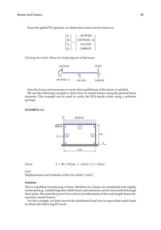
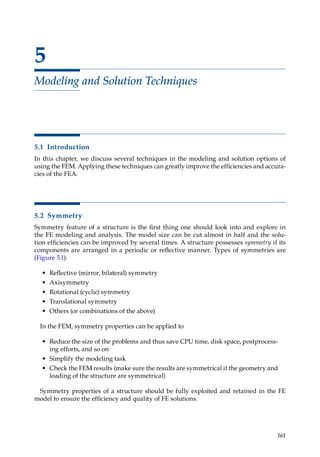
180. 165
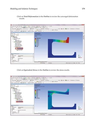
Modeling and Solution Techniques
(1) + 4x(2) ⇒ (2):
( )
( )
( )
1
2
3
8 2 0
0 14 12
0 3 3
2
2
3
−
−
−
−










|
|
|
|
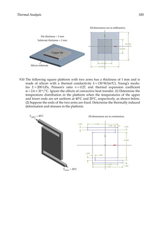
(5.3)
(2) +
14
3
(3) ⇒ (3)
( )
( )
( )
1
2
3
8 2 0
0 14 12
0 0 2
2
2
12
−
− −










|
|
|
|
(5.4)
Back substitutions (to obtain the solution):
x
x x
.
x x
3
2 3
1 2
12 2 6
2 12 14 5
1 5
5
6
2 2 8
= =
= − + = =










= + =
/
( )/
( )/
or x
1
1 5
.
(5.5)
5.4.4 An Example: Iterative Method
The Gauss–Seidel method (as an example):
Ax = b (A is symmetric) (5.6)
or
a x b i N
ij j i
j
N
= =
=
∑ , , ,...,
1
1 2
Start with an estimate x(0) of the solution vector and then iterate using the following:
x
a
b a x a x
i
k
ii
i ij j
k
ij j
k
j i
N
j
i
( ) ( ) ( )
,
+ +
= +
=
−
= − −








∑
∑
1 1
1
1
1
1
fo
or i N
= 1 2
, ,..., (5.7)
In vector form,
x A b A x A x
( ) ( ) ( )
[ ]
k
D L
k
L
T k
+ − +
= − −
1 1 1
(5.8)
where
AD = 〈aii〉 is the diagonal matrix of A,
AL is the lower triangular matrix of A,

181. 166 Finite Element Modeling and Simulation with ANSYS Workbench
such that
A A A A
= + +
D L L
T
(5.9)
Iterations continue until solution x converges, that is
x x
x
( ) ( )
( )
k k
k
+
−
≤ ε
1
(5.10)
where ε is the tolerance for convergence control.
Iterative solvers with moderate selections of the tolerance are usually much faster than
direct solvers in solving large-scale models. However, for ill-conditioned systems, direct
solvers should be applied to ensure the accuracy of the solutions.
5.5 Nature of Finite Element Solutions
FEA model is a mathematical model of the real structure, based on many approximations.
An observation is made on the FEA models and solutions:
• Real structure—infinite number of nodes (physical points or particles), thus infi-
nite number of DOFs
• FEA model—finite number of nodes, thus finite number of DOFs
In particular, one can argue that the displacement field is controlled (or constrained) by
the values at a limited number of nodes (Figure 5.4).
Therefore, we have the so-called stiffening effect:
• FEA model is stiffer than the real structure.
• In general, displacement results are smaller in magnitudes than the exact values.
Hence, the FEM solution of displacement is a lower bound of the exact solution.
Recall that on an element:
4
α = 1
u = Nα uα
Σ
FIGURE 5.4
Elements in an FEA model.

182. 167
Modeling and Solution Techniques
That is, FEA displacement solutions approach the exact solution from below (Figure 5.5),
which can be used to monitor the FEA solutions. However, this is true only for the dis-
placement-based FEA (which is the FEA formulation discussed in this book).
5.6 Convergence of FEA Solutions
As the mesh in an FEA model is “refined” (with smaller and smaller elements) repeatedly,
the FEA solution will converge to the exact solution of the mathematical model of the prob-
lem (the model based on beam, plane stress/strain, plate, shell, or 3-D elasticity theories or
assumptions). Several types of refinements have been devised in the FEA, which include:
h-refinement: Reduce the size of the element (“h” refers to the typical size of the
elements).
p-refinement: Increase the order of the polynomials on an element (linear to qua-
dratic, and so on; “p” refers to the highest order in a polynomial).
r-refinement: Rearrange the nodes in the mesh.
hp-refinement: Combination of the h- and p-refinements (to achieve better results).
With any of the above type of refinements, the FEA solutions will converge to the ana-
lytical solutions of the mathematical models. Some FEA software can automate the process
of refinements in the FEA solutions to achieve the so-called adaptive solutions.
5.7 Adaptivity (h-, p-, and hp-Methods)
Adaptive FEA represents the future of the FEA applications. With proper error control,
automatic refinements of an FEA mesh can be generated by the program until the con-
verged FEA solutions are obtained. With the adaptive FEA capability, users’ interactions
Exact solution
FEA solutions
No. of DOFs
Δ (Displacement)
FIGURE 5.5
Convergence of FEM solutions with exact solution.

183. 168 Finite Element Modeling and Simulation with ANSYS Workbench
are reduced, in the sense that a user only needs to provide a good initial mesh for the
model (even this step can be done by the software automatically).
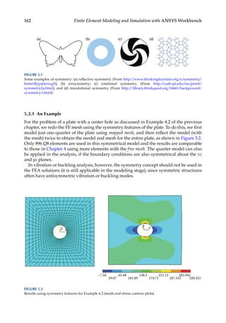
Error estimates are crucial in the adaptive FEA. Interested readers can refer to Reference
[5] for more details. In the following, we introduce one type of the error estimates.
We first define two stress fields:
σ—element by element stress field (discontinuous across elements)
σ*—averaged or smoothed stress field (continuous across elements)
Then, the error stress field can be defined as
σE = σ − σ* (5.11)
Compute strain energies,
U U U
= = σ σ
=
−
∑ ∫
i
i
M
i
T
V
dV
i
1
1
1
2
, E (5.12)
U U U
* * * * *
,
= = σ σ
=
−
∑ ∫
i
i
M
T
V
i
i
dV
1
1
1
2
E (5.13)
U U U
E Ei
i
M
Ei E
T
E
V
dV
i
= = σ σ
=
−
∑ ∫
1
1
1
2
, E (5.14)
where M is the total number of elements and Vi is the volume of the element i.
One error indicator—the relative energy error is defined as
η
+





 ≤ η ≤
=
U
U U
E
E
1 2
0 1
/
. ( ) (5.15)
The indicator η is computed after each FEA solution. Refinement of the FEA model con-
tinues until, say
η ≤ 0.05
When this condition is satisfied, we conclude that the converged FE solution is obtained.
Some examples of using different error estimates in the FEA solutions can be found in
Reference [5].
5.8 Case Study with ANSYS Workbench
Problem Description: Garden fountains are popular amenities that are often found at
theme parks and hotels. As a fountain structure is usually an axisymmetric geometry with

184. 169
Modeling and Solution Techniques
axisymmetric loads and support, only a 2-D model, sliced through the 3-D geometry, is
needed to correctly predict the deformation of or stress in the structure. The figure below
gives the cross section of an axisymmetric model of a two-tier garden fountain made of
concrete. Determine the maximum deformation and von Mises stress under the given
hydrostatic pressure. Use adaptive meshing to improve solution convergence.
0.66
0.5
0.8
1
0.6
0.06
0.06
0.2
0.12
0.12
0.1
Material: Concrete
E = 29 GPa
Boundary conditions:
Bottom edge: fixed.
Left edge: axis of symmetry.
Hydro pressure on dotted edges.
(All units are in meter)
ν = 0.15
Solution
To solve the problem with ANSYS Workbench, we employ the following steps:
Step 1: Start an ANSYS Workbench Project
Launch ANSYS Workbench and save the blank project as ‘Fountain.wbpj’.
Step 2: Create a Static Structural Analysis System
Drag the Static Structural icon from the Analysis Systems Toolbox window
and drop it inside the highlighted green rectangle in the Project Schematic
window to create a standalone static structural analysis system.

185. 170 Finite Element Modeling and Simulation with ANSYS Workbench
Step 3: Add a New Material
Double-click on the Engineering Data cell. In the following Engineering Data
interface that appears, click the empty box highlighted below and type
‘Concrete’ as the new material.
Select ‘Concrete’ from the Outline window, and double-click Isotropic Elasticity
under Linear Elastic in the leftmost Toolbox window. Enter 29E9 for Young’s
Modulus and 0.15 for Poisson’s Ratio in the Properties window. Close the
A2: Engineering Data panel.

186. 171
Modeling and Solution Techniques
Step 4: Launch the SpaceClaim Program
Right-click on the Geometry Cell and choose Properties from its context menu to
bring up the Properties of Schematic A3: Geometry panel. In the Properties
panel under Basic Geometric Options, make sure that Surface Bodies is
checked to enable surface modeling. Also, select 2D for Analysis Type in the
panel. Next, double-click on the Geometry cell to launch SpaceClaim.
Step 5: Create Surface Sketch
To customize units, select the SpaceClaim Options from the File menu to view
the SpaceClaim Options window. In the Options window, set Meters as the
unit for Length, and set Minor grid spacing to 0.02 m. Right-click anywhere
in the Graphics Window, and click Select New Sketch Plane from the drop-
down context menu.

187. 172 Finite Element Modeling and Simulation with ANSYS Workbench
Mouse over x-y plane, and click to select the highlighted x-y plane. This will
change the sketch plane from the default x-z plane (shown above) to the x-y
plane (shown below).
Click Plan View on the toolbar to view the sketch grid head-on. Click Sketch
Mode on the Design tab to begin a sketch. Click on the Line icon. Draw a
closed-loop line profile as dimensioned below. When necessary, press the Esc
key to end the line creation.

188. 173
Modeling and Solution Techniques
Note that the dimensions labelled in the above sketch is added by choosing
Dimensions on the Detail tab. To add a dimension, click on an object to place
the dimension at a desired location.
Click the Create Rounded Corner icon on the Design tab. To create a rounded
corner, click one line and click the other intersecting line, and enter a value of
0.1 in the text box for fillet radius R. Repeat this step until all four fillets are
created as shown below. Note that a value of 0.2 m is shown for ∅ during the
fillet creation. This is corresponding to a fillet radius of 0.1m.

189. 174 Finite Element Modeling and Simulation with ANSYS Workbench
Step 6: Create Surface Body
Click the Pull icon on the Design tab. The following Surface will be created based
on the sketch. Exit the SpaceClaim program.
Step 7: Launch the Static Structural Program
Double-click on the Model cell to launch the Static Structural program. Click
on Geometry in the Outline tree. In the Details of “Geometry”, choose
Axisymmetric for the 2D Behavior field.
Click SYSSurface in the Project Outline Tree. In the Details of “SYSSurface”,
click to the right of the Material Assignment field and select Concrete from
the drop-down context menu.

190. 175
Modeling and Solution Techniques
Step 8: Generate Mesh
Right click on Mesh in the Project Outline. Select Insert and then Sizing from
the context menu. In the Details of “Face Sizing”, enter’0.03m’ for the Element
Size. Click on the surface body in the Graphics window and apply it to the
Geometry selection.
Right click on Mesh. Select Insert and then Method. In the Details of “Automatic
Method”, click on the surface body, and apply it to the Geometry selection.
Select Triangles from the drop-down menu of Method. This will allow the use
of triangular elements for the mesh generation.
In the Details of “Mesh”, change the Element Order to Linear. This will specify
the use of linear elements in the mesh. Note that linear triangular elements are
employed here to show the convergence of linear FEA approximate solutions;
they are in general not recommended for stress analysis. Right-click on Mesh
and select Generate Mesh.

191. 176 Finite Element Modeling and Simulation with ANSYS Workbench
Step 9: Apply Boundary Conditions
Right-click on Static Structural (A5). Choose Insert and then Fixed Support
from the context menu. Apply this support to the horizontal line at the
bottom.
Right-click on Static Structural (A5). Choose Insert and then Frictionless Support
from the context menu. Apply this support to the leftmost vertical line (center line
of the fountain). The frictionless support prevents the line from moving or deform-
ing in the normal direction, and thus is equivalent to a symmetry condition.
Step 10: Apply Loads
In the Project Outline, right-click on Static Structural (A5). Choose Insert and
then Hydrostatic Pressure. The hydrostatic load simulates pressure due to
fluid weight.
In the Details of “Hydrostatic Pressure”, ctrl-click the horizontal line and the
adjacent line fillet shown below, and apply the two edges to the Geometry
selection. Enter 1000 kg/m3 for Fluid Density. Change the Define By selec-
tion to Components, and enter 9.8 m/s2 for the Y Component of Hydrostatic
Acceleration. Enter 0.68 m for the X Coordinate and 0.76 m for the Y
Coordinate for the Free Surface Location. The location corresponds to the
upper endpoint of the line fillet.
Insert another Hydrostatic Pressure load, and apply the pressure to the line and
the adjacent line fillet as shown below.

192. 177
Modeling and Solution Techniques
Step 11: Retrieve Solution
Insert a Total Deformation item by right-clicking on Solution (A6) in the Outline
tree.
Right-click on the Total Deformation in the Outline tree, and choose Insert then
Convergence.

193. 178 Finite Element Modeling and Simulation with ANSYS Workbench
In the Details of “Convergence”, enter 1% for the Allowable Change field.
In the Details of “Solution (A6)”, set Max Refinement Loops as 10, and
Refinement Depth as 1. The refinement depth controls the aggressiveness of
the mesh refinement; it has a range from 0 to 3 with a larger number indicating
more aggressive refinement.
Insert an Equivalent Stress item by right-clicking on Solution (A6) in the Outline
tree.
Right-click on Solution (A6) in the Outline tree and choose Solve. The program
will start to iterate the solution until the difference between two consecutive
iterations is less than 1% or the maximum number of mesh refinement loops
reaches 10. After completion, click on Convergence in the Outline to review
the convergence curve. The resulting maximum deformations at different
mesh iterations are also recorded in the table below the curve.

194. 179
Modeling and Solution Techniques
Click on Total Deformation in the Outline to review the converged deformation
results.
Click on Equivalent Stress in the Outline to review the stress results.

195. 180 Finite Element Modeling and Simulation with ANSYS Workbench
Modeling tips: A model may be subjected to body forces such as gravitational or
radial centrifugal/inertia forces, in addition to the hydrostatic pressure load.
To consider such forces, the density of the structure’s material needs to be
given as an input, and the forces are typically calculated as follows:
f r
f g
r
z
=
= −
ρ ω
ρ
2
, ;
,
equivalentradialcentrifugal/inertialforce
gr
ravitationalforce;
where ρ is the mass density and g the gravitational acceleration (=9.8 m/s2).
Take the following steps to add body forces to the fountain model. First, double-
click on Density in Physical Properties Toolbox. Enter 2.38e3 for Density in
the Properties of Outline Row 3: Concrete.
Next, refresh the Model cell of Project Schematic after the above change is made
on the Engineering Data cell. Double-click on the Model cell to launch the
Static Structural Program.
In the Project Outline shown below, right-click on Static Structural (A5). Choose
Insert and then Standard Earth Gravity.

196. 181
Modeling and Solution Techniques
Right-click on Static Structural (A5) and choose Insert then Rotational Velocity.
In the Details of “Rotational Velocity”, change Define By to Components. Enter
5 rad/s for Y Component.

197. 182 Finite Element Modeling and Simulation with ANSYS Workbench
Right-click on Solution (A6) in the Outline tree, and select Solve to update the
model results. The new deformation and stress results are shown below. Both
the maximum deformation and the maximum von Mises stress values are
shown to be slightly increased, as compared to the results considering only the
hydrostatic pressure load.
5.9 Summary
In this chapter, we discussed a few modeling techniques and options related to FEA solu-
tions. For static analysis of symmetrical structures, the symmetry features should be
explored in both the modeling (meshing) stage and the solution stage (if the BCs are sym-
metrical as well). Substructuring or using SEs is a useful technique for solving large-scale
problems with constrained computing resources. Convergence of the FEA solutions is the
important goal in FEA and should be monitored by using the error estimates and employ-
ing the adaptive FEA capabilities in the software. The showcase using ANSYS Workbench is
introduced to show how to apply the various techniques introduced in this chapter.

198. 183
Modeling and Solution Techniques
5.10 Review of Learning Objectives
Now that you have finished this chapter you should be able to
1. Apply symmetry in meshing and analysis for a symmetrical structure.
2. Apply axisymmetric model and elements when the structure and loads are
axisymmetric.
3. Select proper equation solvers (direct or iterative) for the FE model at hand.
4. Understand the sources of errors in FEA and the error indicators.
5. Know how to refine a mesh using h-refinement or p-refinement.
6. Apply the various techniques in the FEA of a model using ANSYS Workbench.
PROBLEMS
5.1 Consider the two plate structures shown below. The structures are symmetri-
cally loaded on the x–y plane. Use symmetry to construct appropriate finite
element models for the structures, indicating load and support conditions.
F F
q
q
5.2 For a tapered bar shown below, study the deformation and stresses in the bar
with a 2-D model using axisymmetric elements and a 1-D model using bar
elements in ANSYS Workbench. Assume R1 = 1 m, R2 = 0.5 m, L = 5 m, force
F = 3000 N, Young’s modulus E = 200 GPa, and Poisson’s ratio ν = 0.3. The bar is
fixed at the left end. Compare the results from the 2-D and 1-D models.
L
R2
2R1
F
5.3 Anopencylindershownbelowhasaninnerradiusa = 1 m,outerradiusb = 1.1 m,
length L = 6 m, and is applied with a pressure load p = 10 GPa on the inner sur-
face. The outer surface of the cylinder is prevented from radial deformation, and
the cylinder is free to deform along the length direction. Compute the stresses
in the cylinder using a 2-D axisymmetric model in ANSYS Workbench. Assume
Young’s modulus E = 200 GPa and Poisson’s ratio ν = 0.3.

199. 184 Finite Element Modeling and Simulation with ANSYS Workbench
a
b L
5.4 The rotating part sketched below is made of steel with Young’s modulus
E = 200 GPa, Poisson’s ratio ν = 0.3, and mass density ρ = 7850 kg/m3. Assume
that the part is rotating at a speed of 100 RPM about the z axis. Ignore the gravi-
tational force. Compute the stresses in the part using an axisymmetric model in
ANSYS Workbench.
z
ω
5 mm 8 mm
30 mm 16 mm
12
mm
30
mm
50
mm
5.5 Determine the deformation and stress distributions for a solid cylinder under
the influence of the gravity force and radial centrifugal force using ANSYS
Workbench. The cylinder is made of aluminum with Young’s modulus E = 73 GPa,
Poisson’s ratio ν = 0.3, and mass density ρ = 2800 kg/m3. Assume that the
part is rotating at a speed of 50 rad/s about its central axis. Radius = 10 mm,
height = 20 mm, angular velocity around cylinder central axis = 50 rad/s.
10 mm
ω
20
mm
5.6 Suppose that we need to find out the in-plane effective modulus of a composite
reinforced with long fibers aligned in the z-direction and distributed uniformly.
A 2-D elasticity model shown below can be used for this study with ANSYS
Workbench. The effective modulus can be estimated by using the formula
Eeff x ave x ave
= σ ε
( ) ( )
/ , where the averaged stress and strain are evaluated along the
vertical edge on the right side of the model. Assume for the matrix E = 10 GPa,

200. 185
Modeling and Solution Techniques
ν = 0.35, and for the fibers E = 100 GPa, ν = 0.3. The unit cell has a dimension of
1 × 1 μm2 and the radius of the fibers is 0.2 μm.
Start with 1 × 1 cell, 2 × 2 cells, 3 × 3 cells, … and keep increasing the number
of the cells as you can. Report the value of the effective Young’s modulus of the
composite in the x direction. Employ symmetry features of the model in gener-
ating the meshes for your analysis.
p
x
y
One unit cell
5.7 Suppose that a “meshed panel” will be used in a design in order to reduce the
weight. For this purpose, we need to find out the in-plane effective modulus of
this panel in the x- or y-direction. A sample piece of the panel similar to the one
shown below can be used for this study. Employ symmetry and study the effects
of the numbers of cells used in the model on the effective modulus of the panel
in the x-direction.
p
x
y a b
One cell
c
Assume the panel is made of aluminum with E = 70 GPa, ν = 0.35, a = 10 mm,
b = 5 mm, c = 1.5 mm, and thickness t = 1 mm.

202. 187
6
Plate and Shell Analyses
6.1 Introduction
Many structure members can be categorized as plates and shells, which are extensions of
the 1-D straight beams and curved beams to 2-D cases, respectively. Examples of struc-
tures that can be modeled as plates are shear walls, floor panels, and shelves, while those
that can be modeled as shells include shell structures in nature (such as sea shells and egg
shells), various containers, pipes, tanks, roofs of buildings (such as the superdome), and
bodies of cars, boats, and aircrafts. Figure 6.1 shows an airplane (Boeing 787) that is con-
structed mainly using plate and shell structure members.
The advantages of using plate and shell structures are their light weight, superior load-
carrying capabilities, and sometimes, simply their artistic appeals.
6.2 Review of Plate Theory
Plates are flat surfaces applied with lateral loading, with bending behaviors dominating
the structural response. Shells are structures which span over curved surfaces; they carry
both membrane and bending forces under lateral loading. The thickness t of a plate or a
shell is much smaller than the other dimensions of the structure. Theories related to plates
and shells are briefly reviewed below.
6.2.1 Force and Stress Relations in Plates
Consider an infinitesimally small element in a plate under lateral loading. The internal
shear forces and bending moments acting on the element, and the induced stresses are
shown below in Figure 6.2 and Figure 6.3, respectively.
The induced stresses are related to the internal moments and forces in the following
manner:
Bending moments (per unit length):
M zdz N m m
x x
t
t
= σ ⋅
−
∫ , ( )
/
/
2
2
/ (6.1)

203. 188 Finite Element Modeling and Simulation with ANSYS Workbench
Mxy
Mx
Qx
Mxy
My
Qy
x
y
z
Mid-surface
q(x, y)
t
∆x
∆y
FIGURE 6.2
Forces and moments acting on an infinitesimally small element in a plate.
σx
τxz
x
y
z
τxy
σy
τxy
τyz
FIGURE 6.3
Stresses acting on the infinitesimally small element in the plate.
FIGURE 6.1
An airplane made of numerous plate and shell structures.

204. 189
Plate and Shell Analyses
M zdz N m m
y y
t
t
= σ ⋅
−
∫ , ( )
/
/
2
2
/ (6.2)
Twisting moment (per unit length):
M zdz N m m
xy xy
t
t
= τ ⋅
−
∫ , ( )
/
/
2
2
/ (6.3)
Shear Forces (per unit length):
Q dz N m
x xz
t
t
= τ
−
∫ , ( )
/
/
2
2
/ (6.4)
Q dz N m
y yz
t
t
= τ
−
∫ , ( )
/
/
2
2
/ (6.5)
Maximum bending stresses:
( ) , ( )
max max
σ = ± σ = ±
x
x
y
y
M
t
M
t
6 6
2 2 (6.6)
Similar to the beam model, there is no bending stress at the mid-surface and the maxi-
mum/minimum stresses are always at z = ±t/2.
6.2.2 Thin Plate Theory (Kirchhoff Plate Theory)
The thin plate theory is based on assumptions that a straight line normal to the mid-
surface remains straight and normal to the deflected mid-surface after loading (Figure
6.4); that is
γxz = γyz = 0 (Negligible transverse shear deformations)
x
z
w
∂w
∂x
FIGURE 6.4
Deflection and rotation after loading of a plate according to Kirchhoff plate theory.

205. 190 Finite Element Modeling and Simulation with ANSYS Workbench
The displacement, strains, and stresses can be written in terms of the main variable—
deflection w = w(x, y), as follows:
Displacement:
w w x y deflection
u z
w
x
v z
w
y
=
= −
∂
∂
= −
∂
∂
( , ), ( )
(6.7)
Strains:
ε = −
∂
∂
ε = −
∂
∂
γ = −
∂
∂ ∂
x
y
xy
z
w
x
z
w
y
z
w
x y
2
2
2
2
2
2
(6.8)
Note that there is no stretch of the mid-surface caused by the deflection of the plate.
Stresses (plane stress state):
σ
σ
τ










=
− ν
ν
ν
− ν










ε
ε
γ



x
y
xy
x
y
xy
E
1
1 0
1 0
0 0 1 2
2
( )/ 







(6.9)
or,
σ
σ
τ










= −
−
ν
ν
− ν










∂
∂
∂
∂
x
y
xy
z
E
w
x
w
1
1 0
1 0
0 0 1
2
2
2
2
ν
( )
y
y
w
x y
2
2
∂
∂ ∂






















(6.10)
The following equation governs the equilibrium of the plate in the z-direction:
D w q x y
∇ =
4
( , ) (6.11)
where
∇ ≡
∂
∂
+
∂
∂ ∂
+
∂
∂






4
4
4
4
2 2
4
4
2
x x y y

206. 191
Plate and Shell Analyses
D
Et
=
−
3
2
12 1
( )
( )
ν
the bending rigidity of the plate (6.12)
q = lateral distributed load (force per unit area).
Note that Equation 6.11 is of analogous form with the following 1-D equation for straight
beam:
EI
d w
dx
q x
4
4
= ( ) (6.13)
The fourth-order partial differential equation, given in Equation 6.11 and in terms of
the deflection w(x,y), needs to be solved under certain given boundary conditions. Typical
boundary conditions for plate bending include:
Clamped: w
w
n
=
∂
∂
=
0 0
, (6.14)
Simply supported: w Mn
= =
0 0
, (6.15)
Free: Q M
n n
= =
0 0
, (6.16)
where n is the normal direction of the boundary (Figure 6.5). Note that the given values in
the boundary conditions shown above can be nonzero values as well.
6.2.2.1 Example: A Thin Plate
A square plate (Figure 6.6) with four edges clamped or hinged, and under a uniform load
q or a concentrated force P at the center C.
For this simple geometry, Equation 6.11 with the boundary condition of Equation 6.14 or
6.15 can be solved analytically. The maximum deflections are given in Table 6.1 for the four
different cases. These values can be used to verify the FEA solutions.
n
s
Boundary
FIGURE 6.5
The boundary of a plate.

207. 192 Finite Element Modeling and Simulation with ANSYS Workbench
6.2.3 Thick Plate Theory (Mindlin Plate Theory)
If the thickness t of a plate is not small, for example, when t/L ≥ 1/10 (L = a characteristic
dimension of the plate main surface), then the thick plate theory by Mindlin should be
applied. The theory accounts for the angle changes within a cross section, that is
γ γ
xz yz
≠ ≠
0 0
, ( )
transverse shear deformations
This means that a line which is normal to the mid-surface before the deformation will
not be so after the deformation (Figure 6.7).
The new independent variables θx and θy are rotation angles of a line, which is normal to
the mid-surface before the deformation, about x- and y-axis, respectively.
The following new relations hold:
u z v z
y x
= θ = − θ
, (6.17)
x
y
z
Given: E, t, and ν = 0.3
C
L
L
FIGURE 6.6
A square plate.
TABLE 6.1
Deflection at the Center (with D = Et3/(12(1 − v2)))
Clamped Simply Supported
Under uniform load q 0.00126 qL4/D 0.00406 qL4/D
Under concentrated force P 0.00560 PL2/D 0.0116 PL2/D
x
z
w
θy –
∂w
∂x
∂w
∂x
≠
FIGURE 6.7
Displacement and rotation based on the Mindlin thick plate theory.

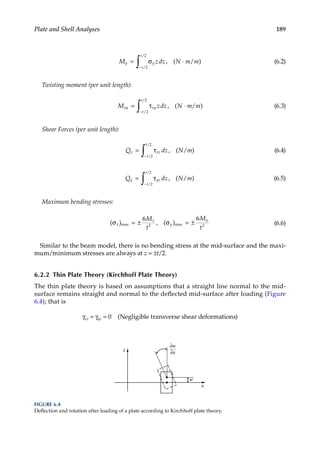
208. 193
Plate and Shell Analyses
and
ε =
∂θ
∂
ε = −
∂θ
∂
γ =
∂θ
∂
−
∂θ
∂






=
∂
∂
+ θ γ
x
y
xz
z
y
z
x
z
y x
w
x
y
x
xy
y x
y y
, ,
,
,
γ z
z x
y
=
∂
∂
− θ
w
(6.18)
Note that if we impose the conditions (or assumptions) that
γ =
∂
∂
+ θ = γ =
∂
∂
− θ =
xz y yz x
w
x
w
y
0 0
, (6.19)
then we can recover the relations applied in the thin plate theory.
The governing equations and boundary conditions can be established for thick plates
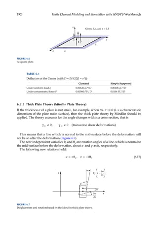
based on the above assumptions, with the three main variables involved being w(x, y),
θx(x, y), and θy(x, y).
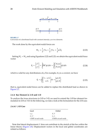
6.2.4 Shell Theory
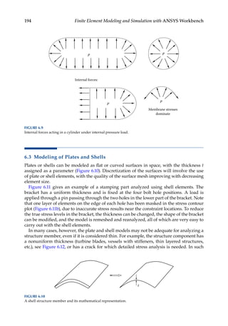
Unlike the plate models, where only bending forces exist, there are two types of forces in
shells, that is, membrane forces (in plane forces) and bending forces (out of plane forces)
(Figures 6.8 and 6.9).
6.2.4.1 Shell Example: A Cylindrical Container
Similar to the plate theories, there are two types of theories for modeling shells, namely
thin shell theory and thick shell theory. Shell theories are the most complicated ones to
formulate and analyze in mechanics. Many of the contributions were made by Russian
scientists in the 1940s and 1950s, due to the need to develop new aircrafts and other light-
weight structures. Interested readers can refer to Reference [6] for in-depth studies on this
subject. These theoretical works have laid the foundations for the development of various
finite elements for analyzing shell structures.
FIGURE 6.8
Forces and moments in a shell structure member.

209. 194 Finite Element Modeling and Simulation with ANSYS Workbench
6.3 Modeling of Plates and Shells
Plates or shells can be modeled as flat or curved surfaces in space, with the thickness t
assigned as a parameter (Figure 6.10). Discretization of the surfaces will involve the use
of plate or shell elements, with the quality of the surface mesh improving with decreasing
element size.
Figure 6.11 gives an example of a stamping part analyzed using shell elements. The
bracket has a uniform thickness and is fixed at the four bolt hole positions. A load is
applied through a pin passing through the two holes in the lower part of the bracket. Note
that one layer of elements on the edge of each hole has been masked in the stress contour
plot (Figure 6.11b), due to inaccurate stress results near the constraint locations. To reduce
the true stress levels in the bracket, the thickness can be changed, the shape of the bracket
can be modified, and the model is remeshed and reanalyzed, all of which are very easy to
carry out with the shell elements.
In many cases, however, the plate and shell models may not be adequate for analyzing a
structure member, even if it is considered thin. For example, the structure component has
a nonuniform thickness (turbine blades, vessels with stiffeners, thin layered structures,
etc.), see Figure 6.12, or has a crack for which detailed stress analysis is needed. In such
t
FIGURE 6.10
A shell structure member and its mathematical representation.
p p
Internal forces:
Membrane stresses
dominate
p
p
FIGURE 6.9
Internal forces acting in a cylinder under internal pressure load.

210. 195
Plate and Shell Analyses
cases, one should turn to 3-D elasticity theory and apply solid elements which will be dis-
cussed in the next chapter.
6.4 Formulation of the Plate and Shell Elements
Several types of finite elements suitable for the analyses of plates and shells are introduced
below.
6.4.1 Kirchhoff Plate Elements
The following four-node quadrilateral element has only bending capabilities. It has three
DOFs at each node, that is, w w y
, ,
∂ ∂
/ and ∂ ∂
w y
/ (Figure 6.13).
FIGURE 6.11
Stress analysis of a bracket using shell elements: (a) the FEA model; (b) stress contour plot.
FIGURE 6.12
Cases in which shell elements are not adequate: (a) casting parts; (b) parts with nonuniform thickness. 3-D solid
elements should be applied in such cases.

211. 196 Finite Element Modeling and Simulation with ANSYS Workbench
On each element, the deflection w(x, y) is represented by
w
w
( , )
x y N w N
x
N
w
y
i i xi
i
yi
i
i
= +
∂
∂





 +
∂
∂














=
∑
1
4
(6.20)
where Ni, Nxi, and Nyi are shape functions. This is an incompatible element [7]. The stiffness
matrix is still of the form
k B EB
=
∫ T
V
dV (6.21)
where B is the strain–displacement matrix and E Young’s modulus (stress–strain)
matrix.
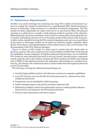
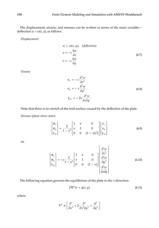
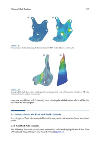
6.4.2 Mindlin Plate Elements
The following two quadrilateral elements are Mindlin types with only bending capabili-
ties (Figure 6.14). There are three DOFs at each node, that is, w, θx, and θy.
On each element, the displacement and rotations are represented by
w x y N w
x y N
x y N
i i
i
n
x i xi
i
n
y i yi
i
n
( , )
( , )
( , )
=
θ = θ
θ = θ
=
=
=
∑
∑
∑
1
1
1
(6.22)
For these elements, there are three independent fields within each element. Deflection
w(x, y) is linear for Q4, and quadratic for Q8.
x
y
z
3
4
Mid-surface
2
2 2
1
t ∂w
w2
,
∂w
∂x ∂y
,
1 1
∂w
w1
,
∂w
∂x ∂y
,
FIGURE 6.13
A four-node quadrilateral element with 3 DOFs at each node.

212. 197
Plate and Shell Analyses
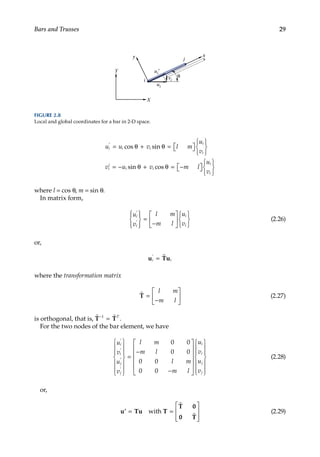
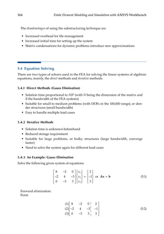
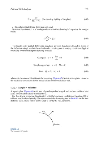
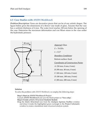
6.4.3 Discrete Kirchhoff Elements
This is a triangular element with only bending capabilities. First, start with a six-node
triangular element (Figure 6.15). There are 5 DOFs at each corner node ( , , ,
w w x w y
∂ ∂ ∂ ∂
/ /
θ θ
x y
, ) 2 DOFs ( , )
θ θ
x y at each mid-node, and a total of 21 DOFs for the six-node element.
Then, impose conditions γxz = γyz = 0, and so on, at selected nodes to reduce the DOFs
(using relations in Equation 6.18), to obtain the following discrete Kirchhoff triangular
(DKT) element (Figure 6.16).
For the three-node DKT element shown above, there are 3 DOFs at each node, that is,
w, θ = ∂ ∂
( )
x w x
/ , and θ = ∂ ∂
( )
y w y
/ , and a total of 9 DOFs for the element. Note that w(x, y)
is incompatible for DKT elements [7]; however, its convergence is faster (w is cubic along
each edge) and it is efficient.
6.4.4 Flat Shell Elements
A flat shell element can be developed by superimposing a plane stress element to a plate
element (Figure 6.17).
x
y
z
1
2
3
4 6
5
FIGURE 6.15
A six-node triangular element with 5 DOFs at each corner node and 2 DOFs at each mid-node.
x
y
z
1 2
3
FIGURE 6.16
Discrete Kirchhoff triangular element with 3 DOFs at each node.
x
y
z
t
1 2
3
4
x
y
z
t
1 2
3
4
5
6
7
8
FIGURE 6.14
Four- and eight-node quadrilateral plate elements.

213. 198 Finite Element Modeling and Simulation with ANSYS Workbench
This is analogous to the combination of a bar element and a simple beam element to
yield a general beam element for modeling curved beams. A flat shell element, with the
DOFs labeled at a typical node i, is shown in Figure 6.18.
6.4.5 Curved Shell Elements
Curved shell elements are based on the various shell theories. They are the most general
shell elements (flat shell and plate elements are subsets). An eight-node curved shell ele-
ment is illustrated in Figure 6.19, with the DOFs labeled at a typical node i. Formulations
of the shell elements are relatively complicated. They are not discussed here and detailed
derivations are available in References [7–9].
u
v
w
θx
θy
FIGURE 6.18
Q4 or Q8 shell elements.
+
Plane stress element
(membrane)
Plate element
(bending)
Flat shell element
FIGURE 6.17
Combination of plane stress and plate bending elements yields a flat shell element.
u
v
w
θx
θy
θz
i
i
FIGURE 6.19
An eight-node curved shell element and the DOFs at a typical node i.

214. 199
Plate and Shell Analyses
6.5 Case Studies with ANSYS Workbench
Problem Description: Vases are decorative pieces that can be of any artistic shapes. The
figure below gives the dimensions of a flower vase made of glass. Assume that the vase
has a uniform thickness of 4 mm. The water level reaches 100 mm below the opening of
the vase. Determine the maximum deformation and von Mises stress in the vase under
the hydrostatic pressure.
80 mm
280
mm
50 mm
D
C
B
E
Material: Glass
E = 70 GPa
ν = 0.17
Boundary Conditions:
Bottom surface: fixed.
Coordinates of Construction Points:
A: (50 mm, 0 mm, 0 mm)
B: (90 mm, 40 mm, 0 mm)
C: (60 mm, 120 mm, 0 mm)
D: (40 mm, 180 mm, 0 mm)
E: (80 mm, 280 mm, 0 mm)
A
Solution
To solve the problem with ANSYS Workbench, we employ the following steps:
Step 1: Start an ANSYS Workbench Project
Launch ANSYS Workbench and save the blank project as ‘Vase.wbpj’.
Step 2: Create a Static Structural Analysis System
Drag the Static Structural icon from the Analysis Systems Toolbox window
and drop it inside the highlighted green rectangle in the Project Schematic
window to create a standalone static structural analysis system.

215. 200 Finite Element Modeling and Simulation with ANSYS Workbench
Step 3: Add a New Material
Double-click on the Engineering Data cell to add a new material. In the follow-
ing Engineering Data interface that appears, click the empty box highlighted
below and type ‘Glass’.
Select ‘Glass’ from the Outline window, and double-click Isotropic Elasticity
under Linear Elastic in the leftmost Toolbox window. Enter 70E9 for Young’s
Modulus and 0.17 for Poisson’s Ratio in the Properties window. Close the
A2: Engineering Data panel.

216. 201
Plate and Shell Analyses
Step 4: Launch the SpaceClaim Program
Right-click on the Geometry Cell and choose Properties from its context menu to
bring up the Properties of Schematic A3: Geometry panel. In the Properties
panel under Basic Geometric Options, make sure that Surface Bodies is
checked to enable surface modeling. Also, select 3D for Analysis Type in the
panel. Next, double-click on the Geometry cell to launch SpaceClaim.

217. 202 Finite Element Modeling and Simulation with ANSYS Workbench
Step 5: Create a Profile Sketch
To customize units, select the SpaceClaim Options from the File menu to view
the SpaceClaim Options window. In the Options window, set Millimeters as
the unit for Length, and set Minor grid spacing to 10mm. Click OK to exit the
Options window.

218. 203
Plate and Shell Analyses
Right-click anywhere in the Graphics Window, and click Select New Sketch
Plane from the drop-down context menu.
Mouse over x-y plane, and click to select the highlighted x-y plane. This will
change the sketch plane from the default x-z plane (shown above) to the x-y
plane (shown below).

219. 204 Finite Element Modeling and Simulation with ANSYS Workbench
Click Plan View on the toolbar to view the sketch grid head-on. Click Sketch
Mode on the Design tab to begin a sketch. Click on the Point icon. Draw five
construction points A, B, C, D and E located as shown below.
Click on the Spline icon on the Design tab. Draw a spline passing through the
five points by clicking A, B, C, D, and finally double-click at E to end the spline
creation.

220. 205
Plate and Shell Analyses
Click on the Line icon on the Design tab. Draw a horizontal line from the origin
O to point A.
Step 6: Create a Surface Body
Click the Pull icon on the Design tab, and select the Revolve icon from the
Graphics window. Click on the Y-axis in the Graphics window to set it as the
axis of revolution, and then click line OA. Click the Full Pull icon to revolve
line OA 360° around the Y-axis. Repeat the same steps for the spline by first
clicking on the Y-axis, and then click on the spline and then click the Full Pull
icon to revolve.

221. 206 Finite Element Modeling and Simulation with ANSYS Workbench
Two Surfaces will be created as shown below. Click on one Surface from the
Structure Tree, and enter 4 for the Midsurface Thickness in the lower left
Properties panel. Repeat the same steps for the other surface.
To check surface normal directions, click the Normal icon in the Quality group
on the Measure tab. Ctrl-click the two surfaces in Graphics Window. The
surface normal direction at the point where you click will be displayed. The
inward pointing arrows shown below indicate incorrect surface normals.

222. 207
Plate and Shell Analyses
Ctrl-click on the two surfaces in the Graphics Window, and right-click on the
highlighted two surfaces and select Reverse Face Normal to flip the surface
normal outward.
Ctrl-click the two Surfaces in the Structure Tree, and right-click Move to New
Component in the context menu.

223. 208 Finite Element Modeling and Simulation with ANSYS Workbench
A Component1 will be created in the Structure Tree with the two surfaces moved
underneath. Click Component1 in the Structure Tree, and change the Share
Topology to Merge in the bottom left Properties menu to merge the 2 surfaces.
After that, close the SpaceClaim program.
Step 7: Launch the Static Structural Program
Double-click on the Model cell to launch the Static Structural program. Ctrl-
click the two Surfaces in the Project Outline Tree. In the Details of “Multiple
Selection”, click to the right of the Material Assignment field and select Glass
from the drop-down context menu.

224. 209
Plate and Shell Analyses
Step 8: Generate Mesh
Right click on Mesh in the Project Outline. Select Insert and then Sizing from
the context menu. In the Details of “Sizing”, enter’5e-3 m’ for the Element
Size. Click on the side wall and the bottom surface of the vase in the Graphics
window and apply them to the Geometry selection.
Right-click on Mesh and select Generate Mesh.

225. 210 Finite Element Modeling and Simulation with ANSYS Workbench
Step 9: Apply Boundary Conditions
Right-click on Static Structural (A5). Choose Insert and then Fixed Support
from the context menu. Apply this support to the bottom surface of the vase.
Step 10: Apply Loads
Right-click on Static Structural (A5). Choose Insert and then Hydrostatic
Pressure. In the Details of “Hydrostatic Pressure”, Ctrl-click the side wall
and the bottom surface of the vase, and apply the two faces to the Geometry
selection. Change the Shell Face to Bottom, because the hydrostatic ­
pressure
is applied to the inside of the shell surface. Enter 1000 kg/m3 for Fluid Density.
Change the Define By selection to Components, and enter 9.8 m/s2 for the Y
Component of Hydrostatic Acceleration. Enter 180e-3 m in the field of Y
Coordinate of the Free Surface Location.

226. 211
Plate and Shell Analyses
Step 11: Retrieve Solution
Insert a Total Deformation item by right-clicking on Solution (A6) in the Outline
tree.
Insert an Equivalent Stress item by right-clicking on Solution (A6) in the Outline
tree.
Right-click on Solution (A6) in the Outline tree and select Solve.
Click on Total Deformation in the Outline to review the deformation results.
Click on Equivalent Stress in the Outline to review the stress results.

227. 212 Finite Element Modeling and Simulation with ANSYS Workbench
Modeling tips: Surface bodies can be created from planar 2D sketches, or by revolv-
ing, extruding or sweeping lines or curves. In many case, they can also be cre-
ated from solid models, by using the Mid-Surface tool provided in Workbench.
For example, a parasolid file of a 3D display shelf geometry is imported into
ANSYS as shown below. In the SpaceClaim Options window, set Millimeters
as the unit for Length.
To create a midsurface geometry, click Midsurface on Prepare tab in SpaceClaim,
and click the Select Faces icon from the Graphics Window. The shelf panel has
a thickness of 3mm. Therefore, in the left Options-Midsurface panel, select Use
range, and enter 2mm for Minimum thickness and 4mm for Maximum thickness.
Click on the solid body in the Graphics window, and click the Check Mark icon.

228. 213
Plate and Shell Analyses
Eighteen surface bodies will be generated based on automatic face pair detection,
and added to the Structure Tree as shown below. Right click on the Midsurface
in the Structure Tree, and click Hide Others. This will hide the solid body and
display only the created midsurfaces.
Next, click Midsurface-Solid1 in the Structure Tree, and change the Share
Topology to Merge in the bottom left Properties menu to merge all the sur-
faces. Exit SpaceClaim program, and the new model is now ready for subse-
quent simulation with plate or shell elements.

229. 214 Finite Element Modeling and Simulation with ANSYS Workbench
6.6 Summary
In this chapter, the main aspects of the plate and shell theories and the plate and shell ele-
ments used for analyzing plate and shell structures are discussed. Plates and shells can
be regarded as the extensions of the beam elements from 1-D line elements to 2-D surface
elements. Plates are usually applied in modeling flat thin structure members, while the
shells are applied in modeling curved thin structure members. In applying the plate and
shell elements, one should keep in mind the assumptions used in the development of these
types of elements. In cases where these assumptions are no longer valid, one should turn
to general 3-D theories and solid elements. A showcase using shell elements in modeling a
vase is introduced using ANSYS Workbench.
6.7 Review of Learning Objectives
Now that you have finished this chapter you should be able to
1. Understand the assumptions used in the plate and shell theories.
2. Understand the behaviors of the plate and shell elements.
3. Know when not to use plate and shell elements in stress analysis (e.g., when plate
or shell structures have nonuniform thickness or small features).
4. Create FEA models using plate and shell elements for deformation and stress anal-
ysis using ANSYS Workbench.
PROBLEMS
6.1 The square plate shown below has the following dimensions and material con-
stants: L = 1 m, t = 0.02 m, E = 30 × 106 N/m2, and ν = 0.3. Use plate elements to
determine the maximum displacement and von Mises stress in the slab in the
following cases: (a) The four edges are clamped and the slab is under a uniform
load q = 1 N/m2. (b) The four edges are clamped and the slab is under a concen-
trated force P = 1 N at the center C. (c) The four edges are hinged and the slab is
under a uniform load q = 1 N/m2. (d) The four edges are hinged and the slab is
under a concentrated force P = 1 N at the center C. Verify the FEA solutions with
the analytical solutions given in the Table 6.1.
x
y
z
C
L
L

230. 215
Plate and Shell Analyses
6.2 The roof structure shown below is loaded by its own weight with q = 90 lbf/
in2. The dimensions and material constants are: R = 25 in., L = 50 in., t = 0.25 in.,
E = 432 × 106 psi, and ν = 0.0. The two straight edges are free, while the two
curved edges have a “diaphragm” support (meaning that x and y DOFs are con-
strained, but z (along the length axis) and all rotational DOFs are unconstrained).
Use shell elements to find the maximum displacement and von Mises stress in
the structure. Verify your results (note that the value of the analytical solution
for the displacement at the mid-point A of the straight edge is 0.3024 in.).
A
R
80°
q
L
6.3 The pinched cylinder shown below is loaded by a force F = 1 N. The dimensions
and material constants are: R = 300 mm, L = 600 mm, t = 3 mm, E = 3 × 106 N/mm2,
and ν = 0.3. Circular ends have diaphragm support (meaning that y and z DOFs
are constrained, but x (along the length axis) and all rotational DOFs are uncon-
strained). Use shell elements to find the maximum displacement and von Mises
stress in the structure. Verify your results (note that the value of the analytical
solution for the displacement at the mid-point A is 0.1825 × 10−4 mm).
R
A
F
F
L/2
L/2
6.4 ThepinchedhemisphereshownbelowhasradialloadsF = 2 Nattheequator.The
dimensionsandmaterialconstantsare:R = 10 m,t = 0.04 m,E = 68.25 × 106 N/m2,
and ν = 0.3. The hemisphere has a free edge, and is restrained only against rigid
body motion. Use shell elements to find the maximum displacement and von
Mises stress in the structure. Verify your results (note that the value of the ana-
lytical solution for the displacement at the point A is 0.0924 m).
F
F
A
F
R
F

231. 216 Finite Element Modeling and Simulation with ANSYS Workbench
6.5 The twisted strip shown below has a load F = 10−6 N. The dimensions and
material constants are: b = 1.1 m, L = 12 m, t = 0.0032 m, E = 29 × 106 N/m2, and
ν = 0.22. The strip has a 90° twist over length L and is cantilevered. Use shell ele-
ments to find the maximum displacement and von Mises stress in the structure.
F
b
L
A
6.6 The twisted strip shown below has a load F = 10−6 N. The dimensions and
material constants are: b = 1.1 m, L = 12 m, t = 0.0032 m, E = 29 × 106 N/m2,
and ν = 0.22. The strip has a 90° twist over length L and is cantilevered. Use
shell elements to find the maximum displacement and von Mises stress in the
structure.
F
b
L
A
6.7 Consider a glass cup placed on a table, as shown in the figure. Using shell ele-
ments, find the maximum displacement and von Mises stress in the cup when
the cup is applied with a pressure load of 10 N/mm2 on the inner wall. Assume
that the cup has a uniform thickness of 4 mm, E = 70 GPa, and ν = 0.17.
40 mm
150
mm
30 mm

232. 217
Plate and Shell Analyses
6.8 Consider a glass fish tank placed on a table, as shown in the figure. Using shell
elements, find the maximum displacement and von Mises stress in the tank
when the tank is full of water. Assume that the tank has a uniform thickness of
4 mm, E = 70 GPa, and ν = 0.17.
60 mm
60 mm
100 mm
6.9 A fuel tank, with a total length = 5 m, diameter = 1 m, and thickness = 0.01 m, is
shown below. Assume Young’s modulus E = 200 GPa and Poisson’s ratio ν = 0.3.
Using shell elements, find the deformation and stresses when the tank is applied
with an internal pressure p = 1 MPa and placed on the ground.
6.10 A bookshelf shown below is placed on the ground. Assume Young’s modulus
E = 13.1 GPa, Poisson’s ratio ν = 0.29, and the shelf thickness t = 6 mm. Using
shell elements, find the deformation and stresses when the bookshelf is applied
with a downward uniform pressure p = 500 N/m2 on the entire surface of the
bookshelf middle layer.
30 cm 30 cm
50 cm 30 cm
20 cm
20 cm

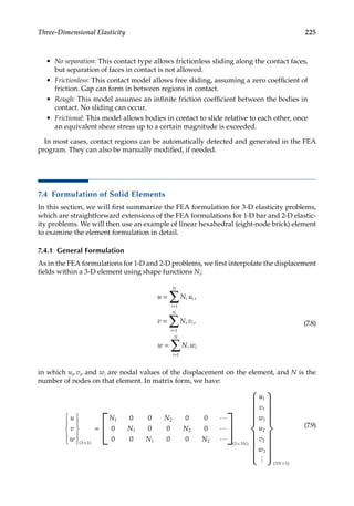
234. 219
7
Three-Dimensional Elasticity
7.1 Introduction
Engineering designs involve 3-D structures that cannot be adequately represented using
1-D or 2-D models. Solid elements based on 3-D elasticity [10,11] are the most general ele-
ments for stress analysis when the simplified bar, beam, plane stress/strain, plate/shell
elements are no longer valid or accurate. In general, 3-D structural analysis is one of the
most important and powerful ways of providing insight into the behavior of an engi-
neering design. In this chapter, we will review the elasticity equations for 3-D and then
discuss a few types of finite elements commonly used for 3-D stress analysis. Several dif-
ferent types of supports, loads, and contact constraints will be introduced for 3-D struc-
tural modeling, followed by a case study on predicting the deformation and stresses in
an assembly structure using ANSYS® Workbench.
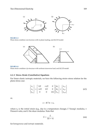
7.2 Review of Theory of Elasticity
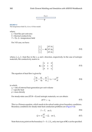
The state of stress at a point in a 3-D elastic body is shown in Figure 7.1.
In vector form, the six independent stress components determining the state of stress
can be written as
σ σ
σ
σ
σ
τ
τ
τ
σ
= { } =






















x
y
z
xy
yz
zx
ij
, [ ]
or
(7.1)

235. 220 Finite Element Modeling and Simulation with ANSYS Workbench
Similarly, the six independent strain components in 3-D can be expressed as
ε ε
ε
ε
ε
γ
γ
γ
ε
= =










{ } , [ ]
x
y
z
xy
yz
zx
ij
or
(7.2)
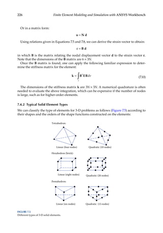
7.2.1 Stress–Strain Relation
The stress–strain relation in 3-D is given by
σ
σ
σ
τ
τ
τ
x
y
z
xy
yz
zx
E
v v
v v v






















=
+ −
−
( )( )
1 1 2
1 0 0 0
v
v v v
v v v
v
v
v
1 0 0 0
1 0 0 0
0 0 0
1 2
2
0 0
0 0 0 0
1 2
2
0
0 0 0 0 0
1 2
2
−
−
−
−
−

















































ε
ε
ε
γ
γ
γ
x
y
z
xy
yz
zx
(7.3)
σy
σz
σx
τyx
τxy
τxz
τyz
τzy
τzx
y
x
z
y, v
x, u
z, w
FIGURE 7.1
State of stress at a point in a 3-D elastic body.

236. 221
Three-Dimensional Elasticity
Or in a matrix form:
σ ε
= E
7.2.2 Displacement
The displacement field can be described as
u =










=










u x y z
v x y z
w x y z
u
u
( , , )
( , , )
( , , )
u1
2
3
(7.4)
7.2.3 Strain–Displacement Relation
Strain field is related to the displacement field as given below
ε
∂
∂
ε
∂
∂
ε
∂
∂
γ
∂
∂
∂
∂
γ
∂
∂
∂
∂
γ
∂
x y z
xy yz xz
u
x
v
y
w
z
v
x
u
y
w
y
v
z
u
= = =
= + = + =
, , ,
, ,
∂
∂
∂
∂
z
w
x
+
(7.5)
These six equations can be written in the following index or tensor form:
ε
∂
∂
∂
∂
ij
i
j
j
i
u
x
u
x
i j
= + =
( )
1
2
1 2 3
, , , ,
Or simply,
εij i j j i
u u
= +
1
2
( ) (
, , Tensor notation)
7.2.4 Equilibrium Equations
The stresses and body force vector f at each point satisfy the following three equilibrium
equations for elastostatic problems:
∂σ
∂
∂τ
∂
∂τ
∂
∂τ
∂
∂σ
∂
∂τ
∂
∂τ
∂
∂
x xy xz
x
yx y yz
y
zx
x y z
f
x y z
f
x
+ + + =
+ + + =
+
0
0
,
,
τ
τ
∂
∂σ
∂
zy z
z
y z
f
+ + = 0
(7.6)

237. 222 Finite Element Modeling and Simulation with ANSYS Workbench
Or in index or tensor notation:
σij j i
f
, + = 0
7.2.5 Boundary Conditions
At each point on the boundary Γ and in each direction, either displacement or traction
(stress on the boundary) should be given, that is
u u on specified displacement
t t on specified trac
i i u
i i
=
=
, ( );
, (
Γ
σ
Γ t
tion)
(7.7)
in which the barred quantities denote given values, and the traction (stress on a surface) is
defined by ti ij
=σ nj or in a matrix form:
t
t
t
n
n
n
x
y
z
x xy xz
xy y yz
xz yz z
x
y
z










=











σ τ τ
τ σ τ
τ τ σ










with n being the normal (Figure 7.2).
7.2.6 Stress Analysis
For 3-D stress analysis, one needs to solve equations in Equations 7.3, 7.5, and 7.6 under
the BCs in Equation 7.7 in order to obtain the stress, strain, and displacement fields (15
equations for 15 unknowns for a 3-D problem). Analytical solutions are often difficult to
find and thus numerical methods such as the FEA are often applied in 3-D stress analysis.
7.3 Modeling of 3-D Elastic Structures
3-D stress analysis using solid elements is one of the most challenging tasks in FEA. In
the following, practical considerations in 3-D FEA modeling such as mesh and BCs are
discussed. The types of contact used in assembly analyses are presented.
Γ (= Γu + Γσ)
Γσ
p
n
Γu
FIGURE 7.2
The boundary of a 3-D elastic domain.

238. 223
Three-Dimensional Elasticity
7.3.1 Mesh Discretization
Meshing structures with complicated geometries can be very tedious and time-­
consuming. Great care should be taken to ensure that the FEA mesh is in good quality
(e.g., with no distorted elements). Computing cost is another factor. For structures with
stress concentrations, large FEA models are often needed, which can run hours or days. A
good CAE engineer should be able to decide where to apply a fine mesh and where not to,
in order to strike a balance between the computational cost and accuracy for an FEA task.
Figure 7.3 shows an example of an FEA model using solid elements of a drag link in a
car. Although the structure has a slender shape, it has a bended angle and holes. 3-D solid
elements are needed for the stress analysis in this case. Great care is taken in meshing this
part, where quadratic elements are used for better accuracy in the stress analysis. Buckling
analysis may also be conducted for slender structures when they are under compressions.
More information about buckling analysis using FEA can be found in Chapter 12.
Figure 7.4 shows a 3-D FEA of a gear coupling which is applied to transmit power
through two aligned rotating shafts. Contact stresses and failure modes are to be deter-
mined based on detailed 3-D FE models. This analysis requires the use of nonlinear FEA
options, which are readily available now in almost all FEA software packages.
7.3.2 Boundary Conditions: Supports
A number of support types are available for 3-D structural analysis. The following list
includes three common support conditions.
• Fixed support: Prevent the geometry entity from moving or deforming.
• Frictionless support: Prevent the face geometry from moving or deforming in the
normal direction relative to the face.
• Cylindrical support: Prevent the cylindrical face from moving or deforming in any
combination of radial, axial, or tangential directions relative to the cylinder.
FIGURE 7.3
FEA for a drag link: (a) the model; (b) mesh for the right end; (c) stress distribution due to tension loads applied
at the two ends.

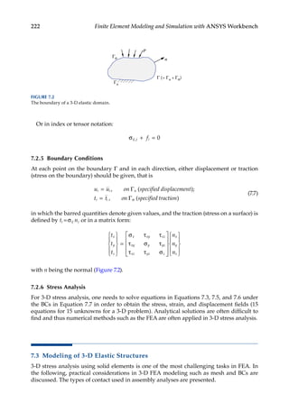
239. 224 Finite Element Modeling and Simulation with ANSYS Workbench
Note that there are six rigid-body motions for 3-D bodies: three translations and three
rotations. These rigid-body motions (causes of singularity of the system of equations) must
be removed from the FEA model for stress analysis to ensure the accuracy of the analysis.
On the other hand, over constraints can also cause inaccurate or unwarranted results. For
more information on the support conditions, please refer to the Mechanical User Guide of
the ANSYS help documents [12].
7.3.3 Boundary Conditions: Loads
The types of structural loads that can be encountered in 3-D analyses include force, moment,
pressure, bearing load, and so on. Inertia loads such as acceleration, standard earth grav-
ity, or rotational velocity may have nontrivial effect on structures’ stress behaviors as well.
Other loading types such as thermal, electric, or magnetic loads can also be involved, but
are less common. For more information on the structural loads, please see Reference [12].
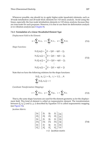
7.3.4 Assembly Analysis: Contacts
For assembly analysis, contact conditions are needed to describe how different contacting
bodies can move relative to one another.
The following types of contact are available for assembly analysis, as listed in Reference
[12]:
• Bonded: This is the default configuration. Bonded regions can be considered as
glued together, allowing no sliding or separation between the contacting regions.
For many applications, bonded contact is sufficient for stress calculations between
bolted or welded parts in assemblies.
FIGURE 7.4
Analysis of a gear coupling: (a) ring gear; (b) hub gear; (c) high-contact stresses in the gear teeth obtained using
nonlinear FEA.

240. 225
Three-Dimensional Elasticity
• No separation: This contact type allows frictionless sliding along the contact faces,
but separation of faces in contact is not allowed.
• Frictionless: This contact model allows free sliding, assuming a zero coefficient of
friction. Gap can form in between regions in contact.
• Rough: This model assumes an infinite friction coefficient between the bodies in
contact. No sliding can occur.
• Frictional: This model allows bodies in contact to slide relative to each other, once
an equivalent shear stress up to a certain magnitude is exceeded.
In most cases, contact regions can be automatically detected and generated in the FEA
program. They can also be manually modified, if needed.
7.4 Formulation of Solid Elements
In this section, we will first summarize the FEA formulation for 3-D elasticity problems,
which are straightforward extensions of the FEA formulations for 1-D bar and 2-D elastic-
ity problems. We will then use an example of linear hexahedral (eight-node brick) element
to examine the element formulation in detail.
7.4.1 General Formulation
As in the FEA formulations for 1-D and 2-D problems, we first interpolate the displacement
fields within a 3-D element using shape functions Ni:
u N u
v N v
w N w
i i
i
N
i
i
N
i
i
i
N
i
=
=
=
=
=
=
∑
∑
∑
1
1
1
,
, (7.8)
in which ui, vi, and wi are nodal values of the displacement on the element, and N is the
number of nodes on that element. In matrix form, we have:
u
v
w
N N
N N
N N
N










×





 ×
( ) ( )
3 1
1 2
1 2
1 2
0 0 0 0
0 0 0 0
0 0 0 0
3 3
=
u
u
v
w
u
v
w
N
1
1
1
2
2
2
3 1













 ×
( )
(7.9)

241. 226 Finite Element Modeling and Simulation with ANSYS Workbench
Or in a matrix form:
u = N d
Using relations given in Equations 7.5 and 7.8, we can derive the strain vector to obtain:
ε = B d
in which B is the matrix relating the nodal displacement vector d to the strain vector ε.
Note that the dimensions of the B matrix are 6 × 3N.
Once the B matrix is found, one can apply the following familiar expression to deter-
mine the stiffness matrix for the element:
k B EB
=
∫ T
v
dv (7.10)
The dimensions of the stiffness matrix k are 3N × 3N. A numerical quadrature is often
needed to evaluate the above integration, which can be expensive if the number of nodes
is large, such as for higher-order elements.
7.4.2 Typical Solid Element Types
We can classify the type of elements for 3-D problems as follows (Figure 7.5) according to
their shapes and the orders of the shape functions constructed on the elements:
Tetrahedron:
Hexahedron (brick):
Pentahedron:
Linear (four nodes) Quadratic (10 nodes)
Linear (eight nodes) Quadratic (20 nodes)
Linear (six nodes) Quadratic (15 nodes)
FIGURE 7.5
Different types of 3-D solid elements.

242. 227
Three-Dimensional Elasticity
Whenever possible, one should try to apply higher-order (quadratic) elements, such as
10-node tetrahedron and 20-node brick elements for 3-D stress analysis. Avoid using the
linear, especially the four-node tetrahedron elements in 3-D stress analysis, because they
are inaccurate for such purposes. However, it is fine to use them for deformation analysis
or in vibration analysis (see Chapter 8).
7.4.3 Formulation of a Linear Hexahedral Element Type
Displacement Field in the Element:
u N u v N v w N w
i i
i
i i i i
i
i
= = =
= =
=
∑ ∑
∑
1
8
1
8
1
8
, , (7.11)
Shape Functions:
N
N
N
1
2
3
1
8
1 1 1
1
8
1 1 1
( , , ) ( )( )( ),
( , , ) ( )( )( ),
ξ η ζ ξ η ζ
ξ η ζ ξ η ζ
= − − −
= + − −
(
( , , ) ( )( )( ),
( , , ) ( )( )( )
ξ η ζ ξ η ζ
ξ η ζ ξ η ζ
= + + −
= − + +
1
8
1 1 1
1
8
1 1 1
8
N
(7.12)
Note that we have the following relations for the shape functions:
Ni j j j ij
i
i
i j
N
( , , ) , , , , .
( , , )
ξ η ζ δ
ξ η ζ
= =
=
=
∑
, 1 2 8
1
1
8
…
Coordinate Transformation (Mapping):
x N x y N y z N z
i i i i
i
i
i i
i
= = =
=
= =
∑
∑ ∑
, ,
1
8
1
8
1
8
(7.13)
That is, the same shape functions are used for the element geometry as for the displace-
ment field. This kind of element is called an isoparametric element. The transformation
between (ξ, η, ζ) and (x, y, z) described by Equation 7.13 is called isoparametric mapping
(see Figure 7.6).
Jacobian Matrix:
∂
∂ξ
∂
∂η
∂
∂ζ
∂
∂ξ
∂
∂ξ
∂
∂ξ
∂
∂η
∂
∂η
∂
∂η
∂
∂
u
u
u
x y z
x y z
x


















=
ζ
ζ
∂
∂ζ
∂
∂ζ
∂
∂
∂
∂
∂
∂
y z
u
x
u
y
u
z




































≡
≡ J Jacobian matrix
(7.14)

243. 228 Finite Element Modeling and Simulation with ANSYS Workbench
Inverting this relation, we have:
∂
∂
∂
∂
∂
∂
∂
∂ξ
∂
∂η
∂
∂ζ
u
x
u
y
u
z
u
u
u


















=












−
J 1







=
=
∑
, with and so on
∂
∂ξ
∂
∂ξ
u N
u
i
i
i
1
8
(7.15)
and similarly for v and w. These relations lead to the following expression for the strain:
ε
ε
ε
ε
γ
γ
γ
∂
∂
∂
∂
∂
∂
∂
∂
∂
=






















=
+
x
y
z
xy
yz
zx
u
x
v
y
w
z
v
x
u
u
∂
∂
∂
∂
∂
∂
∂
∂
∂
y
w
y
v
z
u
z
w
x
+
+


































= u
use( . )
6 15 =Bd
4
1 2
3
8
5 6
7
x
Mapping (xyz ξηζ)
(–1≤ ξ,η,ζ ≤ 1)
2 (1, –1, –1)
3 (1, 1, –1)
η
(–1, 1, –1) 4
6 (1, –1, 1)
7 (1, 1, 1)
(–1, 1, 1) 8
(–1, –1, –1) 1
(–1, –1, 1) 5
o
ξ
ζ
FIGURE 7.6
Mapping an element to the natural coordinate system.

244. 229
Three-Dimensional Elasticity
where d is the nodal displacement vector, that is:
ε = Bd (7.16)
Strain energy is evaluated as
U = =
=
=








∫ ∫
∫
∫
1
2
1
2
1
2
1
2
σ ε ε ε
ε ε
T
V
T
V
T
V
T T
V
dV dV
dV
dV
( )
E
E
d B E B d (7.17)
That is, the element stiffness matrix is
k B EB
=
∫ T
V
dV (7.18)
In ξηξ coordinates:
dV d d d
= (det )
J ξ η ζ (7.19)
Therefore,
k B EB J
=
−
−
−
∫
∫
∫ T
d d d
(det ) ξ η ζ
1
1
1
1
1
1
(7.20)
It is easy to verify that the dimensions of this stiffness matrix is 24 × 24.
Stresses:
To compute the stresses within an element, one uses the following relation once the
nodal displacement vector is known for that element:
σ ε
= =
E EBd
Stresses are evaluated at selected points (Gaussian points or nodes) on each element.
Stress values at the nodes are often discontinuous and less accurate. Averaging of the
stresses from surrounding elements around a node is often employed to smooth the stress
field results.
The von Mises stress for 3-D problems is given by
σ σ σ σ σ σ σ σ
e VM
= = − + − + −
1
2
1 2
2
2 3
2
3 1
2
( ) ( ) ( ) (7.21)
where σ1, σ2, and σ3 are the three principal stresses.

245. 230 Finite Element Modeling and Simulation with ANSYS Workbench
7.4.4 Treatment of Distributed Loads
Distributed loads need to be converted into nodal forces using the equivalent energy con-
cept as discussed in earlier chapters. Figure 7.7 shows the result of a pressure load con-
verted into nodal forces for a 20-node hexahedron element. Note the direction of the forces
at the four corner nodes, which is not intuitive at all.
7.5 Case Studies with ANSYS Workbench
Problem Description: A base stand assembly includes a base, a holder and a pin, as shown
in the following figure. The stand assembly is made of structural steel. Assume a no-sep-
aration condition for all contact regions. Determine the deformation and von Mises stress
distributions of the assembly under the given load and boundary conditions.
Material: Structural steel (E= 200 GPa, ν = 0.3)
Boundary conditions:
The bottom faces of the leg base are fixed.
A downward force of 1 kN is applied to the holder’s top face.
Geometry construction:
The bottom of the hub base is 35 mm above the ground level.
The holder is 36 mm tall, 18 mm of which is in contact with
the hub base.
Sketch of the leg base (extrude
5 mm on both sides)
8.000
R40.000
R50.000
R6.000
R3.000
60.000
R10.000
Sketch of the hub base (extrude
35 mm on one side)
Sketch of the pin (extrude
15 mm on both sides)
Holder
Pin
Base
pA/3 pA/12
p
Surface area = A Nodal forces for 20-node
brick element
FIGURE 7.7
Equivalent nodal forces on a 20-node brick element for a pressure load p.

246. 231
Three-Dimensional Elasticity
Solution
To solve the problem with ANSYS Workbench, we employ the following steps:
Step 1: Start an ANSYS Workbench Project
Launch ANSYS Workbench and save the blank project as ‘Assembly.wbpj’.
Step 2: Create a Static Structural (ANSYS) Analysis System
Drag the Static Structural (ANSYS) icon from the Analysis Systems Toolbox
window and drop it inside the highlighted green rectangle in the Project
Schematic window to create a standalone static structural analysis system.
Step 3: Launch the SpaceClaim Program
Double-click the Geometry cell to launch SpaceClaim. To customize units, select
the SpaceClaim Options from the File menu to view the SpaceClaim Options
window. In the Options window, set Millimeters as the unit for Length, and
set Minor grid spacing to 5mm. Click OK to exit the Options window.

247. 232 Finite Element Modeling and Simulation with ANSYS Workbench

248. 233
Three-Dimensional Elasticity
Step 4: Create the Base Geometry
Click Plan View on the toolbar to view the sketch grid head-on. Click Sketch Mode on
the Design tab to begin a sketch. Click on the Rectangle icon. Draw a 10mm × 10mm
rectangle with its center located 45mm away horizontally from the origin.
Click the Circular Pattern icon to create a circular pattern of rectangles. In the
lower left Options panel, set Circular Count as 3. In the Graphics Window,
click on the rectangular surface, and then click on the Y-axis as the axis to
generate pattern about. Click the Checkmark icon to create the pattern.

249. 234 Finite Element Modeling and Simulation with ANSYS Workbench
Click on the Pull icon on the Design tab. In the Graphics Window, click on the
rectangular surface as shown below. Then, click on the Pull Direction icon,
and click on the Z-axis.
Next, click on the Revolve icon right next to the highlighted Z-axis to set it as the
axis to revolve the pattern about. In the Graphics Window, Pull the surface
pattern up along the yellow pull arrow, and enter 90 degrees in the text box as
shown below to generate the tripod base geometry.

250. 235
Three-Dimensional Elasticity
Click on Home view, and click the Sketch mode icon. Mouse over x-z plane in
the Graphics Window, and click anywhere in the Graphics Window to set
x-z plane as the sketch plane. Draw a circle with a diameter of 12 mm on it, as
shown below.
Draw another concentric circle with a diameter of 20mm on the plane, as shown
below.

251. 236 Finite Element Modeling and Simulation with ANSYS Workbench
Click the Pull icon, and click on the annulus ring shape from the Graphics
­window to highlight the selection.
Pull up the annulus ring shape 70mm above the ground level.

252. 237
Three-Dimensional Elasticity
In the Graphics Window, rotate the geometry for a better view, and click on the
annulus ring shape on the bottom to highlight the selection.
Pull up the annulus ring shape 35mm above the ground level, as shown below.

253. 238 Finite Element Modeling and Simulation with ANSYS Workbench
Right-click anywhere in the Graphics Window, and select View and Top in the
context menu. Note that the tripod base geometry is not hollow in the center.
Click on the circular area in the Graphics Window. Select Cut in the lower left
Options panel.

254. 239
Three-Dimensional Elasticity
Pull up the circular area more than 70mm high above the ground level to make a
hollow circular shaft in the middle, as shown below.
Now click on the Solid item in the Structure Tree to highlight the selection in the
Graphics Window. Note that the solid part only contains the center cylinder,
and it does not include the three legs.

255. 240 Finite Element Modeling and Simulation with ANSYS Workbench
To merge parts, click on the Combine icon in the Design tab. In the Graphics
Window, click on the center cylinder, and then click the Select Bodies to
Merge icon. Next, click on the three legs in the Graphics Window to merge
them together with the cylinder geometry.
Click on the Solid item in the Structure Tree to highlight the selection in the
Graphics Window. Note that the solid part now represents the merged geom-
etry of the tripod base.

256. 241
Three-Dimensional Elasticity
Step 5: Create the Holder and Pin Geometry
In the Graphics Window, click on the annulus ring shape at the top of the tripod
base to highlight the selection as shown below.
Click on the Sketch Mode icon. This will create a sketch plane on the annulus ring
surface. Click the Circle icon, and draw a circle with a diameter of 12mm, as
shown below.

257. 242 Finite Element Modeling and Simulation with ANSYS Workbench
Click on the Pull icon, and click on the circular surface highlighted as shown
below. Click on the Pull Both Sides icon in the lower left Options panel.
Pull the circular area up with a total depth of 36mm. Since the area is pulled in
both directions, the pulling distance in each direction is only 18mm, which is
half of the total depth of 36mm.

258. 243
Three-Dimensional Elasticity
Click on the Sketch Mode icon. Mouse over the y-z plane in the Graphics
Window, and click to highlight the selection. This will change the sketch plane
to the y-z plane.
Right-click anywhere in the Graphics Window, and select View and Right in the
context menu. Click on the Circle icon, and draw a circle with a diameter of
6mm and centered 60mm vertically above the origin.

259. 244 Finite Element Modeling and Simulation with ANSYS Workbench
Click on the Pull icon. Click on the Surface item in the Structure Tree to highlight
the circular surface. Click on the Pull Both Sides icon in the lower left Options
panel.
Pull the circular surface along the yellow pull arrow for a total length of 30mm,
as shown below. Click on Solid in the Structure Tree. A merged base stand
geometry is now created.

260. 245
Three-Dimensional Elasticity
Step 6: Create the Three-Part Assembly
To create the assembly, the solid geometry needs to be split into three parts. Click
on the Split Body icon. In the Graphics Window, click on the solid part to
highlight the selection as the target object. Click on the cylindrical surface
(highlighted in yellow) to use as a cutter plane.
The solid part will be split into two parts as shown below. Right-click on the first
Solid and rename the part as Pin in the Structure Tree.

261. 246 Finite Element Modeling and Simulation with ANSYS Workbench
Click on the Split Body icon. Click on Solid1 in the Structure Tree to highlight
the selection as the target object. Click on the cylindrical surface (highlighted
in yellow) to use as a cutter plane.
The geometry will be split into three parts as shown below. Right-click on the
second and third items in the Structure Tree and rename them as Holder and
Base, respectively.

262. 247
Three-Dimensional Elasticity
Step 7: Launch the Static Structural Program
Double-click on the Model cell to launch the Static Structural program. ANSYS
Workbench automatically detects contacts between parts of an assembly, whether
it is created in SpaceClaim or imported from neutral geometry files. Click on
Contacts under Connections in the Outline tree. In the Details of “Contact
Regions”, change the Type to No Separation for all three contact regions. No
separation contact prevents gap forming between the contact regions; a small
amount of frictionless sliding may occur along the contact faces.
Step 8: Generate Mesh
Right click on Mesh in the Project Outline. Select Insert and then Sizing from the
context menu. In the Details of “Body Sizing”, enter’2.5e-3 m’ for the Element
Size. Ctrl-click on the three parts in the Graphics window and apply the bod-
ies to the Geometry selection.

263. 248 Finite Element Modeling and Simulation with ANSYS Workbench
Right-click on Mesh and select Generate Mesh.
Step 9: Apply Boundary Conditions
Right-click on Static Structural (A5). Choose Insert and then Fixed Support
from the context menu. Ctrl-click on the three faces highlighted below and
apply them to the Geometry selection in the Details of “Fixed Support”.

264. 249
Three-Dimensional Elasticity
Step 10: Apply Loads
Right-click on Static Structural (A5). Choose Insert and then Force. In the
Details of “Force”, apply the circular face shown below to the Geometry selec-
tion. Change the Define By selection to Components, and enter -1000 N for the
Y Component.
Step 11: Retrieve Solution
Insert a Total Deformation item by right-clicking on Solution (A6) in the Outline
tree.
Insert an Equivalent Stress item by right-clicking on Solution (A6) in the Outline
tree.
Right-click on Solution (A6) in the Outline tree and select Solve.
Click on Total Deformation in the Outline to review the deformation results.

265. 250 Finite Element Modeling and Simulation with ANSYS Workbench
Click on Equivalent Stress in the Outline to review the stress results.
To view deformation of the pin, insert a Total Deformation item by right-clicking
on Solution (A6) in the Outline tree. Click on the pin body in the Graphics
window and apply it to the selection of Geometry in the Details of “Total
Deformation 2”.

266. 251
Three-Dimensional Elasticity
To view stress in the pin, insert an Equivalent Stress item by right-clicking on
Solution (A6) in the Outline tree. Click on the pin body in the Graphics win-
dow and apply it to the selection of Geometry in the Details of “Equivalent
Stress 2”.
Repeat the last two steps to add a Total Deformation 3 and an Equivalent Stress
3 to the Outline. Select the holder body in the Graphics window for the
Geometry selection in both Details of “Total Deformation 3” and Details of
“Equivalent Stress 3”.
Right-click on Solution (A6) in the Outline tree and select Evaluate All Results.
Click on Total Deformation 2 and Total Deformation 3 in the Outline to
review the deformation of the pin and the holder, respectively.

267. 252 Finite Element Modeling and Simulation with ANSYS Workbench
Click on Equivalent Stress 2 and Equivalent Stress 3 in the Outline to review the
von Mises stress of the pin and the holder, respectively.
Modeling tips: It is in general a good idea to take advantage of symmetry when-
ever possible to simplify calculations. The base stand assembly is symmetric
about the XY-plane. To create a half-symmetry model, open “Assembly.wbpj”
and double-click on the Geometry cell in the Project Schematic to launch
the SpaceClaim program. In SpaceClaim, click on the Split By Plane icon on
the Prepare tab. In the Graphics Window, Ctrl-click the pin, holder and base
geometry, and click on the X-Y plane as the cutter plane to split the assembly
into two halves, as shown below. Click on the Select Regions to Remove icon
in the Graphics Window, and click on the divided half parts to remove half of
the assembly. A half-model will be created as shown below. Exit SpaceClaim.

268. 253
Three-Dimensional Elasticity
Double-click on Model cell in the Project Schematic to launch the Static
Structural – Mechanical program. Click Yes on the popup menu to allow
reading the modified upstream data. Click on Contacts under Connections
in the Outline tree. In the Details of “Contact Regions”, change the Type to
No Separation for all three contact regions.
Right-click on Mesh in the Outline and select Generate Mesh. Next, update the
face geometry selection for the Fixed Support boundary condition.

269. 254 Finite Element Modeling and Simulation with ANSYS Workbench
In the half-model, the magnitude of the force applied to a face should be divided
by two. Change the Y Component of the force from -1000 N to -500 N in the
Details of “Force”.
The frictionless support is equivalent to a symmetry condition. Right-click on
Static Structural (A5). Choose Insert and then Frictionless Support from
the context menu. In the Details of “Frictionless Support”, Ctrl-click the
seven faces in the Graphics window as shown below, and apply them to
the Geometry selection field. Note that this step is especially important for
imported geometry with cut faces at the symmetry plane, because the pro-
gram cannot automatically detect symmetry regions as in the case of geometry
created internally.

270. 255
Three-Dimensional Elasticity
Right-click on Static Structural (A5) and select Solve. Click on the deformation
and stress results under Solution (A6) and compare them with results from
the full model.
7.6 Summary
In this chapter, we discussed the 3-D solid elements for elasticity problems, that is, general
3-D deformation and stress analyses. Solid elements are the most accurate elements and
should be applied when the bar, beam, plane stress/strain, and plate/shell elements are no
longer valid or accurate. For stress concentration problems, higher-order solid elements,
such as 10-node tetrahedron or 20-node hexahedron (brick) elements, should be employed
in the FEA. For solids having symmetrical features, symmetric FEA models can be more
effective and efficient.
7.7 Review of Learning Objectives
Now that you have finished this chapter you should be able to
1. Understand the FE formulations for 3-D stress analysis
2. Know the behaviors of the 3-D (tetrahedron and hexahedron) elements
3. Create quality mesh over solids for 3-D stress analysis
4. Perform detailed stress analysis of 3-D structures using ANSYS Workbench
PROBLEMS
7.1 For a tapered bar shown below, study the deformation and stresses in the bar
with a 3-D model using solid elements and a 1-D model using 1-D bar ele-
ments. Assume R1 = 1 m, R2 = 0.5 m, L = 5 m, force F = 3000 N, Young’s modulus

271. 256 Finite Element Modeling and Simulation with ANSYS Workbench
E = 200 GPa, and Poisson’s ratio ν = 0.3. The bar is fixed at the left end. Compare
the FEA results between the 3-D and 1-D models.
L
R2
2R1
F
7.2 An open cylinder shown below has an inner radius a = 1 m, outer radius
b = 1.1 m, length L = 10 m, and is applied with a pressure load p = 10 GPa on the
inner surface. Compute the stresses in the cylinder using shell and solid mod-
els. Compare the FEA results based on these models. Assume Young’s modulus
E = 200 GPa and Poisson’s ratio ν = 0.3.
a
b L
7.3 For the rotating part sketched below, assume that it is made of steel with Young’s
modulus E = 200 GPa, Poisson’s ratio ν = 0.3, and mass density ρ = 7850 kg/m3.
Assume that the part is rotating at a speed of 100 RPM about the z axis. Ignore
the gravitational force. Compute the deformation in the part using the FEA
with a full 3-D model. Compare the 3-D results with the axisymmetric model-
ing results obtained in Problem 5.4.
z
ω
5 mm 8 mm
30 mm 16 mm
12
mm
30
mm
50
mm
7.4 The following figure shows a simple bracket made of structural steel with
Young’s modulus E = 200 GPa and Poisson’s ratio ν = 0.3. The bracket has a
cross-section profile shown below and an extrusion depth of 12 cm. A through-
hole of diameter 1.5 cm is centered on the bracket’s flat ends, one on each side,
as shown in the figure. Suppose that the bracket is fixed on the bottom, and

272. 257
Three-Dimensional Elasticity
lifted by a pressure load of 1000 N/cm2 from the inside surface of the top flat
portion. Compute the deformation and stresses in the bracket using the FEA.
10.000
1.500
1.500
R3.000
8.000 1.500
12.000
8.000
1.500
1.500
All dimensions are in
centimeters.
7.5 The following figure shows a lifting bracket made of structural steel with Young’s
modulus E = 200 GPa and Poisson’s ratio ν = 0.3. The base portion of the bracket
is 20 cm long, 12 cm wide, and 3 cm deep. The fillet radius at the base corners is
1.75 cm. Four through-holes each of radius 1 cm are located symmetrically both
length wise and width wise in the base, with the hole centers being 12 cm apart
by 6 cm apart. The upper portion of the base has a profile sketch shown below
and is 3 cm thick. Suppose that the bracket is fixed on the bottom, and lifted
by a bearing load of 20 kN through the bolt hole located in the upper portion.
Compute the deformation and stresses in the bracket using the FEA.
R3.000
3.000
8.000
3.000
6.000
6.000
R1.500 All dimensions are in
centimeters.
7.6 The following figure shows a bracket made of structural steel with Young’s
modulus E = 200 GPa and Poisson’s ratio ν = 0.3. The rectangular base of the

273. 258 Finite Element Modeling and Simulation with ANSYS Workbench
bracket is 12 cm long, 6 cm wide, and 3 cm deep. The midsection has an over-
all extrusion depth of 1.6 cm and a profile sketch shown below. The hollow
cylinder has an inner radius of 1 cm, an outer radius of 2 cm, and a height
of 4 cm. The central axis of the cylinder is 12.5 cm away from the leftmost
end of the bracket. Suppose that the bracket is fixed on the left end, and is
applied by a pressure load of 60 N/cm2 on the inclined face of the midsec-
tion. Compute the deformation and stresses in the bracket using the FEA.
4.000
8.000
6.000
All dimensions are in
centimeters.
7.7 The following figure shows an S-shaped wooden block with Young’s modulus
E = 70 K N/mm2 and Poisson’s ratio ν = 0.3. The block has a uniform thickness
of 6 mm and a depth of 8 mm. It is fixed on the bottom and subjected to a sur-
face pressure of 1 N/mm2 on the top. Compute the deformation and stresses in
the block using the FEA.
6.000
6.000
6.000
6.000
6.000
24.000
All dimensions are in
centimeters.

274. 259
Three-Dimensional Elasticity
7.8 The following figure shows an L-shaped bracket made of structural steel
with Young’s modulus E = 200 GPa and Poisson’s ratio ν = 0.3. The 4 cm thick
L-shape with a cross-section profile shown in the figure is rigidly connected to
a rectangular base of size 3 cm × 8 cm × 1 cm. Suppose that the bracket is fixed
on the right end at the base. A uniform pressure of 100 N/cm2 is applied on the
protruding surface of the L-shape as shown below. Compute the deformation
and stresses in the bracket using the FEA.
1.000
8.000
3.000
R1.000
1.000
All dimensions are in
centimeters.
7.9 The following two-bar assembly consists of four components made of struc-
tural steel with Young’s modulus E = 200 GPa, Poisson’s ratio ν = 0.3, and den-
sity ρ = 7850 kg/m3. As shown in the figure below, the two bars are identical in
size. Each bar has a diameter of 2 cm and a length of 16 cm. The two identical
end blocks each has a thickness of 2 cm and a fillet radius of 1 cm at the round
corners. The distance of the gap in between the two blocks is 8 cm. Suppose that
the two blocks are fixed on the bottom. The bars are pulled by a pressure load of
100 N/cm2 in opposite directions as shown below. Compute the stresses in the
assembly using the FEA.
All dimensions are in centimeters
Use bonded contact for all contact regions.
5.000
2.000
R1.000
10.000
6.000
All dimensions are in centimeters.
Use bonded contact for all contact regions.
5.000
2.000
R1.000
10.000
6.000
7.10 The following figure shows a half model of a clevis assembly consisting of a
yoke, a pin, and a u-shape. The assembly components are made of structural

275. 260 Finite Element Modeling and Simulation with ANSYS Workbench
steel with Young’s modulus E = 200 GPa and Poisson’s ratio ν = 0.3. The pro-
file sketches of the yoke and the u-shape are shown in the figure below. Both
components have an extrusion depth of 5 cm. In the half model, the pin has a
diameter of 2 cm and a length of 8 cm, and is centered 2.5 cm away from both
the front and the side faces of the u-shape. Suppose that the yoke is fixed on the
left end, and the u-shape is pulled by a pressure load of 100 N/cm2 on the right
end. Compute the stresses in the assembly using the FEA.
12.000
R1.500
1.500
2.000
2.000
2.500
2.500
2.000
3.000
8.000
R1.000
16.000
1.500
R1.500
3.000
All dimensions are in centimeters.
Use no separation for all contact regions.

276. 261
8
Structural Vibration and Dynamics
8.1 Introduction
Vibration and dynamics are fundamental subjects in engineering. Serious problems may
arise from vibration when a structure is not carefully designed for its dynamic integrity.
Vibration can cause malfunction or break down of machines that exhibit unbalance or mis-
alignment. It can also lead to massive engineering failures such as the collapse of a bridge.
Simulation plays an important role in our ability to understand a structure’s dynamic
behavior. Through modeling, the dynamic characteristics of a structure can be captured
and improved before being put into actual use.
In this chapter, we first review the basic equations and their solutions for structural
vibration and dynamic analysis. Then, we discuss the FEA formulations for solving vibra-
tion and dynamic responses. Guidelines in modeling and solving such problems are pro-
vided, along with a case study in ANSYS® Workbench.
A structure vibrates about an equilibrium position when excited by periodic or arbi-
trary inputs. There are three main types of problems for structural vibration and dynamic
analyses:
• Modal analysis (f(t) = 0)
• Frequency response analysis (f(t) = F sin ωt)
• Transient response analysis (f(t) is arbitrary)
where f(t) is the dynamic force applied on the structure, t the time, and ω the circular fre-
quency (Figure 8.1).
8.2 Review of Basic Equations
We begin with a review of vibration of a single-DOF system, consisting of a mass, a
spring, and a damper as shown in Figure 8.2. Then we will review basic equations
for a multi-DOF system, such as the discrete system resulting from the finite element
discretization.

277. 262 Finite Element Modeling and Simulation with ANSYS Workbench
8.2.1 A Single DOF System
From the free-body diagram (FBD) and Newton’s law of motion (ma = f), we have:
mu f t ku cu
= − −
( )
that is
mu cu k u f t
+ + = ( ) (8.1)
where u is the displacement,
u du dt
= / the velocity, and
u d u dt
= /
2 2
the acceleration.
Free Vibration (no applied force to the mass or f(t) = 0):
Free vibration occurs when a mass is moved away from its rest position due to initial
conditions.
Assuming zero damping (c = 0) in a free vibration, Equation 8.1 becomes:
mu k u
+ = 0 (8.2)
The physical meaning of this equation is: inertia force + elastic/stiffness force = 0.
Although there is no applied force, the mass can have nonzero displacement or experience
vibrations under the initial conditions. To solve for such nontrivial solutions, we assume:
u(t) = U sin ωt
where ω is the circular frequency of oscillation and U the amplitude. Substituting this into
Equation 8.2 yields:
cu
ku
f(t)—force
c—damping
k—stiffness
m—mass
m
m
f = f(t)
k
c
f(t)
x, u
FBD:
FIGURE 8.2
A single DOF system with damping.
f(t)
FIGURE 8.1
A dynamic force applied to the structure.

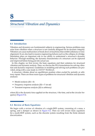
278. 263
Structural Vibration and Dynamics
− ω ω + ω =
U U
2
0
. sin sin
m t k t
that is
[ ]
−ω + =
2
0
m k U
For nontrivial solutions for U, we must have:
[ ]
−ω + =
2
0
m k
which yields
ω =
k
m
(8.3)
This is the circular natural frequency of the single DOF system (rad/s). The cyclic fre-
quency (1/s = Hz) is ω/2π.
Equation 8.3 is a very important result in free vibration analysis, which says that
the natural frequency of a structure is proportional to the square-root of the stiffness
of the structure and inversely proportional to the square-root of the total mass of the
structure.
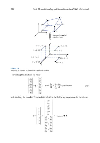
The typical response of the system in undamped free vibration is sketched in Figure 8.3.
For nonzero damping c, where
0 2 2
= ω = =
c c m k m c
c c
( )
critical damping (8.4)
we have the damped natural frequency:
ω = ω −
d 1 2
ξ (8.5)
where
ξ = c cc
/ (8.6)
is called the damping ratio.
u
t
U
U
T = 1/f
u = U sin ωt
FIGURE 8.3
Typical response in an undamped free vibration.

279. 264 Finite Element Modeling and Simulation with ANSYS Workbench
For structural damping: 0 ≤ ξ 0.15 (usually 1 ~ 5%)
ω ≈ ω
d (8.7)
That is, we can ignore damping in normal mode analysis.
The typical response of the system in damped free vibration is sketched in Figure 8.4.
We can see that damping has the effect of reducing the vibration of the system.
8.2.2 A Multi-DOF System
For a multi-DOF system, the equation of motion can be written as
Mu Cu Ku f
+ + = ( )
t (8.8)
in which:
u—nodal displacement vector;
M—mass matrix;
C—damping matrix;
K—stiffness matrix;
f—forcing vector.
The physical meaning of Equation 8.8 is
Inertia forces + Damping forces + Elastic forces = Applied forces
We already know how to determine the stiffness matrix K for a structure, as discussed
in previous chapters. In vibration analysis, we also need to determine the mass matrix and
damping matrix for the structure.
8.2.2.1 Mass Matrices
There are two types of mass matrices: lumped mass matrices and consistent mass matrices. The
former is empirical and easier to determine, and the latter is analytical and more involved
in their computing.
We use a bar element to illustrate the lumped mass matrix (Figure 8.5).
For this bar element, the lumped mass matrix for the element is found to be
u
t
FIGURE 8.4
Typical response of a free vibration with a nonzero damping c cc
.

280. 265
Structural Vibration and Dynamics
m =
ρ
ρ












AL
AL
2
0
0
2
which is a diagonal matrix and thus is easier to compute.
In general, we apply the following element consistent mass matrix:
m N N
= ρ
∫ T
dV
V
(8.9)
where N is the same shape function matrix as used for the displacement field and V is the
volume of the element.
Equation 8.9 is obtained by considering the kinetic energy within an element:
Κ =
=
1
2
1
2
2
u mu
T
mv
(cf.
1
2
)
ρ
ρ = ρ
= ρ
= ρ
∫ ∫
∫
u dV u u dV
dV
V
T
V
T
V
T T
2 1
2
1
2
1
2
( )
( ) ( )
Nu Nu
u N N d
dV
V
∫
m
u
(8.10)
For the bar element (linear shape function), the consistent mass matrix is
m N N
= ρ = ρ
− ξ
ξ





 − ξ ξ

 
 ξ
= ρ


∫ ∫
T
V V
dV AL d
AL
1
1
1 3 1 6
1 6 1 3
/ /
/ /





u
u
1
2
(8.11)
which is a nondiagonal matrix.
Similar to the formation of the global stiffness matrix K, element mass matrices are
established in local coordinates first, then transformed to global coordinates, and finally
assembled together to form the global structure mass matrix M.
2
ρAL ρAL
m1 = m2 =
2
ρ, A, L
1 2
u1 u2
FIGURE 8.5
The lumped mass for a 1-D bar element.

281. 266 Finite Element Modeling and Simulation with ANSYS Workbench
For a simple beam element (Figure 8.6), the consistent mass matrix can be found readily by
applying the four shape functions listed in Equation 3.6. We have:
m N N
= ρ
=
ρ
−
−
−
−
∫ T
dV
AL
L L
L L L L
L L
V
420
156 22 54 13
22 4 13 3
54 13 156 22
1
2 2
3
3 3 22 4
2 2
1
1
2
2
L L L L
v
− −












θ
θ
v
(8.12)
8.2.2.2 Damping
There are two commonly used models for viscous damping: proportional damping (also
called Rayleigh damping) and modal damping.
In the proportional damping model, the damping matrix C is assumed to be proportional
to the stiffness and mass matrices in the following fashion:
C K M
= α + β (8.13)
where the constants α and β are found from the following two equations:
ξ =
α
+
β
ω
ξ =
ω
+
β
ω
1
1
1
2
2
2
2 2 2 2
ω α
, (8.14)
with ω1, ω2, ξ1 and ξ2 (damping ratios) being specified by the user. The plots of the above
two equations are shown in Figure 8.7.
In the modal damping model, the viscous damping is incorporated in the modal equations.
The modal damping can be introduced as
Cφ =
ξ ω
ξ ω
ξ ω












2 0 0
0 2
0 2
1 1
2 2
n n
(8.15)
where ξi is the damping ratio at mode i of a n-DOF system.
θ1 θ2
v2
v1
ρ, A, L
FIGURE 8.6
The consistent mass for a 1-D simple beam element.

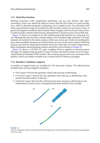
282. 267
Structural Vibration and Dynamics
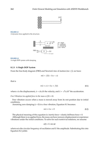
8.3 Formulation for Modal Analysis
Modal analysis sets out to study the inherent vibration characteristics of a structure,
including:
• Natural frequencies
• Normal modes (shapes)
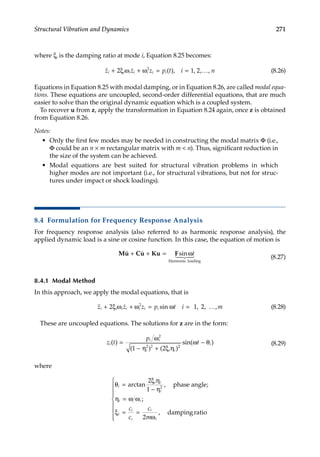
Let f(t) = 0 and C = 0 (ignore damping) in the dynamic Equation 8.8 and obtain:
Mu Ku 0
+ = (8.16)
Assume that displacements vary harmonically with time, that is:
u u
u u
u u
( ) sin( ),
( ) cos( ),
( ) sin( )
t t
t t
t t
= ω
= ω ω
= −ω ω
2
where u is the vector of the amplitudes of the nodal displacements.
Substituting these into Equation 8.16 yields:
[ ]
K M u 0
− ω =
2
(8.17)
Design
spectrum
Frequency
0
0
Damping
ratio
Stiffness-proportional
dampling:
Mass-proportional
dampling:
αω
αω
2ω
, β = 0
, α = 0
2
2
+
ξ2
ξ =
ξ =
ξ =
ξ1
ω1 ω2
β
2ω
β
FIGURE 8.7
Two equations for determining the proportional damping coefficients. (R. D. Cook, Finite Element Modeling
for Stress Analysis, 1995, Hoboken, NJ, Copyright Wiley-VCH Verlag GmbH Co. KGaA. Reproduced with
permission.)

283. 268 Finite Element Modeling and Simulation with ANSYS Workbench
This is a generalized eigenvalue problem (EVP). The trivial solution is u 0
= for any val-
ues of ω (not interesting). Nontrivial solutions ( )
u 0
≠ exist only if:
K M
− ω =
2
0 (8.18)
This is an n-th order polynomial of ω2, from which we can find n solutions (roots) or
eigenvalues ωi (i = 1, 2, …, n). These are the natural frequencies (or characteristic frequen-
cies) of the structure.
The smallest nonzero eigenvalue ω1 is called the fundamental frequency.
For each ωi, Equation 8.17 gives one solution or eigen vector:
[ ]
K M u 0
− ω =
i i
2
ui (i = 1, 2, …, n) are the normal modes (or natural modes, mode shapes, and so on).
Properties of the Normal Modes:
Normal modes satisfy the following properties:
u Ku u Mu
i
T
j i
T
j i j
= =
0 0
, , for ≠ (8.19)
if ω ω
i j
≠ . That is, modes are orthogonal (thus independent) to each other with respect to K
and M matrices.
Normal modes are usually normalized:
u Mu u Ku
i
T
i i
T
i i
= =
1 2
, ω (8.20)
Notes:
• Magnitudes of displacements (modes) or stresses in normal mode analysis have
no physical meaning.
• For normal mode analysis, no support of the structure is necessary.
• ωi = 0 means there are rigid-body motions of the whole or a part of the structure.
This can be applied to check the FEA model (check to see if there are mechanisms
or free elements in the FEA models).
• Lower modes are more accurate than higher modes in the FEA calculations (due
to less spatial variations in the lower modes leading to that fewer elements/wave-
lengths are needed).
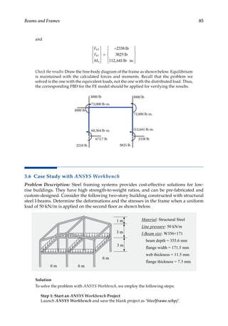
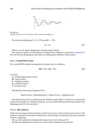
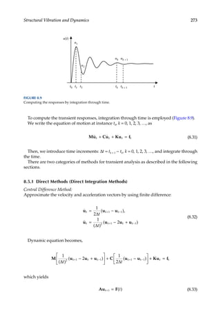
EXAMPLE 8.1
Consider the free vibration of a cantilever beam with one element as shown below.
L
x
1 2
v2
ρ, A, EI
y
θ2

284. 269
Structural Vibration and Dynamics
We have the following equation for the free vibration (EVP):
[ ]
K M
− ω
θ










=







2 2
2
0
0
v
where
K M
=
−
−





 =
ρ −
−






EI
L
L
L L
AL L
L L
3 2 2
12 6
6 4 420
156 22
22 4
,
The equation for determining the natural frequencies is
12 156 6 22
6 22 4 4
0
2 2
− λ − + λ
− + λ − λ
=
L L
L L L L
in which λ = ω ρ
2 4
420
AL EI
/ .
Solving the EVP, we obtain:
ω =
ρ





 θ







=










ω
1 4
1
2
1
3 533
1
1 38
. , . ,
EI
AL L
2
2
v
2
2 4
1
2
2
34 81
1
7 62
=
ρ





 θ







=










. , .
EI
AL
v
L
2
2
The exact solutions of the first two natural frequencies for this problem are
ω =
ρ





 ω =
ρ






1 4
1
2
2 4
1
2
3 516 22 03
. , .
EI
AL
EI
AL
We can see that for the FEA solution with one beam element, mode 1 is calculated
much more accurately than mode 2. More elements are needed in order to compute
mode 2 more accurately. The first three mode shapes of the cantilever beam is shown in
the insert above.
8.3.1 Modal Equations
Use the normal modes (modal matrices), we can transform the coupled system of dynamic
equations to uncoupled system of equations or modal equations.
We have:
[ ] ,
K M u 0
− ω = =
i i i n
2
1, 2, ..., (8.21)
where the normal modes ui satisfy:
u Ku
u Mu
i
T
j
i
T
j
i j
=
=





≠
0
0
,
,
for

285. 270 Finite Element Modeling and Simulation with ANSYS Workbench
and
u Mu
u Ku
i
T
i
i
T
i i
i n
=
= ω





= …
1
1 2
2
,
,
, , ,
for
Form the modal matrix:
Φ = [ ]
( )
n n n
× u u u
1 2 (8.22)
We can verify that:
Φ Φ Ω =
ω
ω
ω














T
K =
0 0
0
0
0 0
Spectral matrix)
1
2
2
2
n
2
(
Φ
Φ =
T
M I
Φ .
(8.23)
Transformation for the displacement vector:
u u u u z
= + + + =
z z zn n
1 1 2 2 Φ (8.24)
where
z =














z t
z t
z t
n
1
2
( )
( )
( )
are called the principal coordinates.
Substitute Equation 8.24 into the dynamic Equation 8.8 and obtain:
M z C z K z f
Φ Φ Φ
+ + = ( )
t
Premultiply this result by ΦT, and apply Equation 8.23:
z C z z p
+ + =
ϕ Ω ( )
t (8.25)
where C I
φ = α + βΩ if proportional damping is applied, and p f
= ΦT
t
( ).
If we employ modal damping:
Cφ =
ξ ω
ξ ω
ξ ω












2 0 0
0 2
0 2
1 1
2 2
n n

286. 271
Structural Vibration and Dynamics
where ξi is the damping ratio at mode i, Equation 8.25 becomes:
z z z p t i n
i i i i i i i
+ ξ ω + ω = = …
2 1 2
2
( ), , , , (8.26)
Equations in Equation 8.25 with modal damping, or in Equation 8.26, are called modal equa-
tions. These equations are uncoupled, second-order differential equations, that are much
easier to solve than the original dynamic equation which is a coupled system.
To recover u from z, apply the transformation in Equation 8.24 again, once z is obtained
from Equation 8.26.
Notes:
• Only the first few modes may be needed in constructing the modal matrix Φ (i.e.,
Φ could be an n × m rectangular matrix with m n). Thus, significant reduction in
the size of the system can be achieved.
• Modal equations are best suited for structural vibration problems in which
higher modes are not important (i.e., for structural vibrations, but not for struc-
tures under impact or shock loadings).
8.4 Formulation for Frequency Response Analysis
For frequency response analysis (also referred to as harmonic response analysis), the
applied dynamic load is a sine or cosine function. In this case, the equation of motion is
Mu Cu Ku F
+ + = ω
sin t
Harmonic loading
(8.27)
8.4.1 Modal Method
In this approach, we apply the modal equations, that is
z z z p t i m
i i i i i i i
+ ω + ω = ω = …
2 1 2
2
ξ sin , , , (8.28)
These are uncoupled equations. The solutions for z are in the form:
z t
p
t
i
i i
i i i
i
( )
( ) ( )
sin( )
=
ω
− η + ξ η
ω − θ
2
2 2 2
1 2
(8.29)
where
θ =
ξ η
− η
η = ω ω
ξ = =
ω
i
i i
i
i i
i
i
c
i
i
c
c
c
m
arctan ,
;
,
2
1
2
2
phase angle;
dam
mpingratio










287. 272 Finite Element Modeling and Simulation with ANSYS Workbench
The response of each mode Zi is similar to that of a single DOF system. Once the natural
coordinate vector z is known, we can recover the real displacement vector u from z using
Equation 8.24.
8.4.2 Direct Method
In this approach, we solve Equation 8.27 directly, that is, compute the inverse of the coef-
ficient matrix, which is in general much more expensive than the modal method.
Using complex notation to represent the harmonic response, we have u u
= ω
ei t
and
Equation 8.27 becomes:
[ ]
K C M u F
+ ω − ω =
i 2
(8.30)
Inverting the matrix [ ],
K C M
+ ω − ω
i 2
we can obtain the displacement amplitude
vector u. However, this equation is expensive to solve for large systems and the matrix
[ ]
K C M
+ ω − ω
i 2
can become ill-conditioned if ω is close to any natural frequency ωi of the
structure. Therefore, the direct method is only applied when the system of equations is
small and the frequency is away from any natural frequency of the structure.
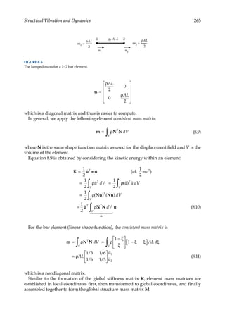
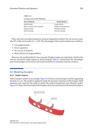
8.5 Formulation for Transient Response Analysis
In transient response analysis (also referred to as dynamic response/time-history ­
analysis),
we are interested in computing the responses of the structures under arbitrary time-­
dependent loading (Figure 8.8).
(a)
(b)
t
f(t)
t
u(t)
FIGURE 8.8
(a) A step type of loading; (b) structural response to the step loading.

288. 273
Structural Vibration and Dynamics
To compute the transient responses, integration through time is employed (Figure 8.9).
We write the equation of motion at instance tk, k = 0, 1, 2, 3, …, as
Mu Cu Ku f
k k k k
+ + = (8.31)
Then, we introduce time increments: Δt = tk + 1 − tk, k = 0, 1, 2, 3, …, and integrate through
the time.
There are two categories of methods for transient analysis as described in the following
sections.
8.5.1 Direct Methods (Direct Integration Methods)
Central Difference Method:
Approximate the velocity and acceleration vectors by using finite difference:
u u u
u u u u
k k k
k k k k
t
t
= −
= − +
+ −
+ −
1
2
1
2
1 1
2 1 1
∆
∆
( ),
( )
( )
(8.32)
Dynamic equation becomes,
M u u u C u u Ku f
1
2
1
2
2 1 1 1 1
( )
( ) ( )
∆ ∆
t t
k k k k k k k
+ − + −
− +





 + −





 + =
which yields
Au F
k t
+ =
1 ( ) (8.33)
t0
u1
u2
uk
tk t
u(t)
uk + 1
tk + 1
t1 t2
FIGURE 8.9
Computing the responses by integration through time.

289. 274 Finite Element Modeling and Simulation with ANSYS Workbench
where
A M C
F f K M u M C
= +
= − −





 − −



1 1
2
2 1 1
2
2
2 2
( )
,
( )
( ) ( )
∆ ∆
∆ ∆ ∆
t t
t
t t t
k k











−
uk 1
We compute uk+1 from uk and uk−1, which are known from the previous time step. The
solution procedure is repeated or marching from t t t t
k k
0 1 1
, , , , ,
… …
+ until the specified max-
imum time is reached. This method is unstable if Δt is too large.
Newmark Method:
We use the following approximations:
u u u u u u
u
k k k k k k
k
t
t
+ + +
+
≈ + + − β + β → =
1
2
1 1
1
2
1 2 2
∆
∆
( )
[( ) ], ( )
≈
≈ + − γ + γ +
u u u
k k k
t
∆ [( ) ]
1 1
(8.34)
where β and γ are chosen constants. These lead to the following equation:
Au F
k t
+ =
1 ( ) (8.35)
where
A K C M
F f C M u u u
= +
γ
β
+
β
= +
∆ ∆
∆
t t
t f t
k k k k
1
2
1
( )
,
( ) ( , , , , , , , , )
γ β
This method is unconditionally stable if
2
1
2
β ≥ γ ≥
For example, we can use γ = =
1 2 1 4
/ /
, ,
β which gives the constant average acceleration
method.
Direct methods can be expensive, because of the need to compute A−1, repeatedly for
each time step if nonuniform time steps are used.
8.5.2 Modal Method
In this method, we first do the transformation of the dynamic equations using the modal
matrix before the time marching:
u u
= =
+ ξ ω + ω = =
=
∑ i i
i
m
i i i i i i i
z t
z z z p t
( ) ,
( ),
1
2
Φz
…
i m.
1, 2, ,
(8.36)

290. 275
Structural Vibration and Dynamics
Then, solve the uncoupled equations using an integration method. We can use, for exam-
ple, 10% of the total modes (m = n/10). The advantages of the modal method are as follows:
• Uncoupled system
• Fewer equations
• No inverse of matrices
• More efficient for large problems
However, the modal method is less accurate if higher modes are important, which is the
case for structures under impact or shock loading. Table 8.1 summarizes the advantages
and disadvantages of the direct and modal methods for transient response analysis.
8.6 Modeling Examples
8.6.1 Modal Analysis
Take a bumper system as an example. Figure 8.10 shows a front bumper and the supporting
brackets in a car. The model is applied to study the dynamic responses of the bumper. Shell
elements were used for this study to obtain the natural frequencies and vibration modes.
Figure 8.11 shows the first mode of the bumper when it is constrained at the bracket locations.
TABLE 8.1
Comparisons of the Methods
Direct Methods Modal Method
Small models Large models
More accurate (with small Δt) Higher modes ignored
Single loading Multiple loading
Shock loading Periodic loading
… …
FIGURE 8.10
FEA model of a front bumper and supporting brackets.

291. 276 Finite Element Modeling and Simulation with ANSYS Workbench
8.6.2 Frequency Response Analysis
Figure 8.12 shows the frequency response of the bumper system by the leftmost curve and
with the acceleration of the two brackets as the input. Several modifications of the bumper
design are also studied with the goal to increase the base natural frequency (e.g., from
below 30 Hz to above 35 Hz) and to reduce the magnitudes of the frequency responses.
The improved responses are shown by the other three curves in Figure 8.12.
8.6.3 Transient Response Analysis
One of the most interesting applications of the transient analysis with FEA is to conduct
crash analysis and virtual drop tests of various products. Figure 8.13 is an example of
crash analysis of a car using the FEA, showing that the bumper system absorbs the
shock energy to help reduce the damage to the car.
8.6.4 Cautions in Dynamic Analysis
• Symmetry model should not be used in the dynamic analysis (normal modes,
etc.) because symmetric structures can have nonsymmetric modes. However,
FIGURE 8.11
The first vibration mode of the bumper.
5.0
Proposed I model (current design)
Proposed III model
Proposed III model
Reference model
4.0
3.0
Total
displacement
(mm)
2.0
1.0
0.0
0.0 10.0 20.0
Frequency (Hz)
30.0 40.0 50.0
FIGURE 8.12
Frequency response of the bumper from 0 to 50 Hz.

292. 277
Structural Vibration and Dynamics
symmetry can still be applied in creating the FEA model of a symmetric
structure.
• Mechanism or rigid body motion means ω = 0. Can use this to check FEA models
to see if they are properly connected and/or supported.
• Input for FEA: Loading F(t) or F(ω) can be very complex and data can be enormous
in real engineering applications (e.g., the load data for a car) and thus they often
need to be filtered first before being used as input for FEA.
• Selecting a proper unit system is very important in vibration or dynamic analysis.
Two choices of the units are listed in Table 8.2. Make sure they are consistent in
the FEA models.
8.7 Case Studies with ANSYS Workbench
Problem Description: Musical instruments such as acoustic guitars create sound by
means of vibration and resonance. The body of an acoustic guitar acts as a resonating
chamber when the strings are set into oscillation at their natural frequencies. The fol-
lowing figure gives the dimensions of a simplified acoustic guitar model. The guitar has
a wall thickness of 3 mm, and is made of Douglas fir wood (E = 13.1 GPa, Poison’s ratio
ν = 0.3, Density = 470 Kg/m3). Assuming the back surface of the guitar is fixed, find the
first ten natural frequencies and plot the first five vibration modes of the guitar. Suppose
a harmonic pressure loading of magnitude 1 MPa is applied to a side wall of the guitar.
Plot the frequency response of the z displacement (along the surface normal direction) of
the front surface.
FIGURE 8.13
Car crash analysis using the FEA. (From LS-Dyna website, http://www.dynaexamples.com/)
TABLE 8.2
Units in Dynamic Analysis
Choice I Choice II
t (time) s s
L (length) m mm
m (mass) kg Mg
a (accel.) m/s2 mm/s2
f (force) N N
ρ (density) kg/m3 Mg/mm3

293. 278 Finite Element Modeling and Simulation with ANSYS Workbench
Material:
Douglas fir (E = 13.1 GPa, ν = 0.3, density
= 470 kg/m3)
Boundary conditions:
A fixed back face; harmonic pressure of
1 MPa applied to a side wall.
Construction point coordinates:
Point x (mm) y (mm)
A 0 0
B 0 10
C 30 70
D 60 80
E 100 70
F 140 50
G 200 60
H 220 50
I 240 10
J 240 0
K 170 0
The guitar profile is a spline that goes
through points A–J.
A circular hole centered at K has a
diameter of 45 mm.
H15
V2
V1 V8
V3 V4
V5 V6 V7
D18
C
B
A
K I
J
D E
F
G
H
H13
H14
H10
H9
H12
H11
H17
H16
Front face
Side wall
Step 1: Start an ANSYS Workbench Project
Launch ANSYS Workbench and save the blank project as ‘Guitar.wbpj’.
Step 2: Create a Modal Analysis System
Drag the Modal icon from the Analysis Systems Toolbox window and drop it
inside the highlighted green rectangle in the Project Schematic window to
create a standalone modal analysis system.
Step 3: Add a New Material
Double-click on the Engineering Data cell to add a new material. In the following
Engineering Data interface which replaces the Project Schematic, type ‘Wood’ as
thenameforthenewmaterial,anddouble-click IsotropicElasticityunderLinear
Elastic in the leftmost Toolbox window. Enter ‘13.1E9’ for Young’s Modulus and

294. 279
Structural Vibration and Dynamics
‘0.3’ for Poisson’s Ratio in the Properties window. Make sure ‘Wood’ is selected
in the Outline of Schematic A2: Engineering Data, and double-click Density
under Physical Properties. Enter ‘470’ for Density in the Properties window.
Close the A2:Engineering Data tab to return to the Project Schematic.
Step 4: Launch the SpaceClaim Program
Right-click on the Geometry Cell and choose Properties from its drop-down con-
text menu to bring up the Properties of Schematic A3: Geometry panel. From
that panel under Basic Geometric Options, select Surface Bodies to enable
surface modeling. Choose 3D as the Analysis Type in the Properties window.
Double-click the Geometry cell to launch SpaceClaim.

295. 280 Finite Element Modeling and Simulation with ANSYS Workbench
Step 5: Create a Profile Sketch
To customize units, select the SpaceClaim Options from the File menu. In the
SpaceClaim Options window that opens, click Units from the left naviga-
tion panel, and select Millimeters for Length. Next, change the Minor Grid
Spacing to 10mm. Click OK.
Click on the Plan View icon to display a heads-on view of the sketch grid. Click
the Point icon on the Design tab. Draw ten construction points A through J, as
shown below. Next, Click the Spline icon, and draw a spline passing through
points A through J; double-click at the last construction point to complete the
spline creation.

296. 281
Structural Vibration and Dynamics
Step 6: Create a Replicate Curve
Click the Mirror icon on the Design tab. In the Graphics Window, click the x-axis,
and then the spline curve as the body to be mirrored. A mirrored spline will
appear as follows.
Step 7: Create an Extruded Body
Click on the Home view icon to change the view to home settings. Click the Pull
icon the Design tab. In the Graphics Window, pull the yellow surface upward

297. 282 Finite Element Modeling and Simulation with ANSYS Workbench
along y-direction, and type 50mm in the box for depth. An extruded solid
body is created as shown below.
Step 8: Create an Extruded Cut on the Top Face
In the Graphics Window, click on the top face of the solid, and click on the Sketch
Mode icon to place the sketch grid on the top face. Click on the Plan View icon
to create a top view of the geometry. Next, click on the Point icon, and create
a point O that is located 170mm horizontally to the left of point A. Then click
on the Circle icon, and draw a circle of diameter 45mm centered at point O.

298. 283
Structural Vibration and Dynamics
Click on Home view. Click on the Pull icon. In the Graphics Window, click on the
circular area on the top face, and pull the surface downward along negative
y-direction to cut a cylindrical hole into the solid. Type 10mm in the textbox for
cut depth. An extruded cut feature is now added as shown below.
Step 9: Create a Surface Body
Click the Shell icon on Design tab. In the Graphics window, click on the circular
face as highlighted below to remove it from the shell. Type 3mm in the box for
shell thickness.

299. 284 Finite Element Modeling and Simulation with ANSYS Workbench
Note that the solid has been turned into a hollow shell. Click on the cylindrical
wall as highlighted below to remove it from the shell. Click the Check Mark
icon to complete the step.
Click on the Midsurface icon on the Prepare tab to prepare for surface modeling.
In the left Options-Midsurface panel, select Use range, and enter 5mm (note
the value entered here needs to be greater than the given guitar thickness of
3mm) for Maximum thickness. Select the body by clicking on the solid geome-
try in the Graphics Window to search for face pairs within the specified offset
range. Click the Check Mark icon to complete the step.

300. 285
Structural Vibration and Dynamics
A midsurface shell model is now created for the guitar. In the Structure Tree,
unselect Solid to view only the surface model in the Graphics Window. Note
that in the lower left Properties panel, Thickness is 3mm for midsurface. Exit
SpaceClaim.
Step 10: Launch the Modal–Mechanical Program
Double-click on the Model cell to launch the Modal–Mechanical program. Click
on the Midsurface item under Geometry in the Project Outline. In the Details
of “Midsurface”, click to the right of the Material Assignment field and select
Wood from the drop-down menu.

301. 286 Finite Element Modeling and Simulation with ANSYS Workbench
Step 11: Generate Mesh
Right click on Mesh in the Project Outline. Select Insert and then Sizing from the
context menu. In the Details of “Face Sizing”, enter’5e-3 m’ for the Element
Size. Click on the front, back, top, bottom faces of the guitar and apply the four
faces to the Geometry selection.
Right-click on Mesh in the Outline, and select Generate Mesh from the context
menu.

302. 287
Structural Vibration and Dynamics
Step 12: Set Up Modal Analysis and Apply Boundary Conditions
Click on Analysis Settings under Modal in the Outline tree. Change the Max
Modes to Find to 10 in the Details of “Analysis Settings”.
Right-click on Modal(A5). Choose Insert and then Fixed Support from the con-
text menu. Apply the bottom face to the Geometry selection.

303. 288 Finite Element Modeling and Simulation with ANSYS Workbench
Step 13: Retrieve Results from Modal Analysis
Insert Total Deformation by right-clicking on Solution (A6) in the Outline.
In the Details of “Total Deformation”, set Mode to 1. Insert another Total
Deformation item. In the Details of “Total Deformation 2”, set Mode to 2.
Repeat this step three more times. Set Mode to 3, 4 and 5, respectively, for each
new insertion. Right-click on Solution (A6) in the Outline and Solve.
Click on Total Deformation in the Outline to review results. The results below
show the first natural frequency of 1083.2 Hz and the corresponding mode
shape.

304. 289
Structural Vibration and Dynamics
Click on Tabular Data and Graph on the right edge of the Graphics window, and
then click on the push pin labeled AutoHide to display the Tabular data and
the Graph as shown below.
The tabular data gives the first 10 natural frequencies of the guitar under the
fixed bottom boundary condition. The play/stop control interface in the
Graph window allows animation of mode shapes. Click on each different
Total Deformation item in the Outline to review results, e.g., the following
figure shows the fourth mode shape, and then exit Modal–Mechanical.

305. 290 Finite Element Modeling and Simulation with ANSYS Workbench
Step 14: Create a Harmonic Response Analysis System
Drag the Harmonic Response icon from the Analysis Systems Toolbox window
and drop it onto the Solution cell of the highlighted Modal system in the
Project Schematic.
This creates a Harmonic Response system that shares data with Modal system
as shown below.

306. 291
Structural Vibration and Dynamics
Step 15: Set Up Harmonic Response Analysis and Assign Loads
Double-click on the Setup cell of the Harmonic Response system to launch the
Multiple Systems–Mechanical program. In the program, select Analysis
Settings from the Outline. Set the Range Minimum to 1000 Hz, Range
Maximum to 4000 Hz, and Solution Intervals to 300. This means that simula-
tion will solve for 300 excitation frequencies with an increment of 10 Hz in the
range from 1000–4000 Hz.
Right-click on Harmonic Response (B5). Choose Insert and then Pressure from
the context menu. In the Details of “Pressure”, set magnitude as 1e6 Pa, and
apply the side face to the Geometry selection.

307. 292 Finite Element Modeling and Simulation with ANSYS Workbench
Step 16: Retrieve Results from Harmonic Response
Right-click on Solution (B6). Choose Insert and Frequency Response and then
Deformation from the context menu. In the Details of “Frequency Response”,
set the Orientation of the Directional Deformation to Y Axis. Click on the face
highlighted in green below and apply it to the Geometry selection.
Right-click on Solution (B6) and select Solve. After solution is done, click on
Frequency Response in the Outline to review the harmonic response of the
guitar.

308. 293
Structural Vibration and Dynamics
Modeling tips: Note that modal analysis can be run as constrained, unconstrained
or partially constrained. Also note that symmetric structure may have asym-
metric modes, and thus, it is not recommended to take advantage of symmetry
to simplify models for modal analysis. In the following, we are going to show
a result comparison between an unconstrained model and the fixed model.
For the unconstrained model, the first six mode shapes obtained from simula-
tion are rigid body modes that allow the structure to move freely. They are not
considered as structural modes. The comparison indicates that a free floating
guitar has a different set of natural frequencies and mode shapes from that of
a fixed guitar. In general, constraint conditions have an effect on the vibration
characteristics of a structure and should be considered carefully when setting
up a model.
The first four structural modes of the unconstrained guitar model.
The first four structural modes of the fixed guitar model.
8.8 Summary
In this chapter, we first reviewed the equations of motion for both single DOF and mul-
tiple DOF systems and discussed how to compute the mass and damping matrices in the
FE formulations. Then, we discussed the methods for solving normal modes, harmonic
responses, and transient responses for structural vibration and dynamic problems. The
advantages and disadvantages of the direct method and modal method are discussed.
Several examples of vibration and dynamic analyses are also discussed to show the appli-
cations of the FEA in vibration and dynamic analyses. The vibration modes of a guitar are
analyzed using ANSYS Workbench.

309. 294 Finite Element Modeling and Simulation with ANSYS Workbench
8.9 Review of Learning Objectives
Now that you have finished this chapter you should be able to
1. Understand the FE formulations for vibration and dynamic analysis of structures
2. Know how to compute the mass and damping matrices in the FE equations of
motion
3. Solve for the natural frequencies and modes of structures using the FEA
4. Compute the harmonic response of structures using the FEA
5. Compute the transient response of structures using the FEA
6. Perform vibration or dynamic analysis of structures using ANSYS Workbench
PROBLEMS
8.1 For the cantilever beam studied in Example 8.1, apply more elements and
investigate the FEA solutions for the first 10 natural frequencies and normal
modes of the beam structure. Assume the beam is made of structural steel
with Young’s modulus E = 200 GPa, Poisson’s ratio ν = 0.3, and mass density
ρ = 7850 kg/m3, and has a length of 100 cm with a 10 cm × 10 cm square cross
section.
8.2 For a square plate with edge length = 1 m, thickness = 0.005 m, Young’s modu-
lus E = 70 GPa, Poisson’s ratio ν = 0.3, and mass density ρ = 2800 kg/m3, find the
first five natural frequencies and normal modes using the FEA when the plate is
a. Clamped at the four edges
b. Simply supported at the four edges
c. Free at the four edges (not supported)
Discuss the effects of the support on the natural frequencies of the plate.
8.3 A fuel tank, with a total length = 5 m, diameter = 1 m, and thickness = 0.01 m,
is shown below. Using the FEA, find the first six natural frequencies and cor-
responding normal modes, when:
a. The tank is not supported at all.
b. The tank is constrained along the circumferences in the radial directions at
the two locations 1 m away from the two ends.

310. 295
Structural Vibration and Dynamics
Carefully build your FE mesh (using shell elements) so that the symmetry of the
tank is reserved and the boundary conditions in part (b) can be applied readily.
Assume the tank is made of steel with Young’s modulus E = 200 GPa, Poisson’s
ratio ν = 0.3, and mass density ρ = 7850 kg/m3.
8.4 For the rotating part sketched below, assume that it is made of steel with
Young’s modulus E = 200 GPa, Poisson’s ratio ν = 0.3, and mass density
ρ = 7850 kg/m3. Ignore the gravitational force. Compute the first five natural
frequencies and normal modes in the part using the FEA when the part is
a. Fixed on the inner cylindrical surface of the hole
b. Fixed on the bottom surface
Compare the results between the two models.
z
ω
5 mm 8 mm
30 mm 16 mm
12
mm
30
mm
50
mm
8.5 The following figure shows a simple plate made of structural steel with Young’s
modulus E = 200 GPa, Poisson’s ratio ν = 0.3, and density ρ = 7850 kg/m3. The
plate has a thickness of 5 mm and is fixed on the left side. Suppose a harmonic
force of magnitude 100 N is applied to the right edge along the plate’s surface
normal direction. Use a solid model and a shell model to compute:
a. The first five natural frequencies and the corresponding normal modes
b. The frequency response of the z directional deformation (along the surface nor-
mal direction of the plate) of the plate surface under the given harmonic load
Compare the results between the two models.
All dimensions are in centimeters.
5.000 R1.000
R5.000 20.000
10.000
10.000
40.000

311. 296 Finite Element Modeling and Simulation with ANSYS Workbench
8.6 ThefollowingfigureshowsasimplebracketmadeofstructuralsteelwithYoung’s
modulus E = 200 GPa, Poisson’s ratio ν = 0.3, and density ρ = 7850 kg/m3. The
bracket has a front face profile shown below and an extrusion depth of 12 cm.
A through-hole of diameter 1.5 cm is centered on the bracket’s flat ends, one on
each side. Suppose that the bracket is fixed on the bottom, and is subjected to a
harmonic pressure load of magnitude 1000 N/cm2 on the top face. Use a solid
model to compute:
a. The first five natural frequencies and the corresponding normal modes
b. The frequency response of the z directional deformation (along the front face
normal direction) of the front face of the bracket under the given harmonic
load
All dimensions are in
centimeters.
Load
10.000
1.500
1.500
1.500
1.500
R3.000
8.000
8.000
12.000
1.500
8.7 The following figure shows an L-shaped bracket made of structural steel with
Young’smodulusE = 200 GPa,Poisson’sratioν = 0.3,anddensityρ = 7850 kg/m3.
The 4 cm thick L-shape with a cross-section profile shown in the figure is rig-
idly connected to a rectangular base of size 3 cm × 8 cm × 1 cm. Suppose that
the bracket is fixed on the right end at the base. A harmonic pressure of mag-
nitude 100 N/cm2 is applied on the protruding surface of the L-shape as shown
below. Using the FEA, compute:
a. The first five natural frequencies and the corresponding normal modes
b. The frequency response of the y directional deformation (along the load
direction) of the bracket’s protruding top face under the given harmonic
load

312. 297
Structural Vibration and Dynamics
All dimensions are in
centimeters.
Load
1.000
R1.000
3.000
8.000
1.000
8.8 The following two-bar assembly consists of four components made of struc-
tural steel with Young’s modulus E = 200 GPa, Poisson’s ratio ν = 0.3, and den-
sity ρ = 7850 kg/m3. As shown in the figure below, the two bars are identical
in size. Each bar has a diameter of 2 cm and a length of 16 cm. The two identi-
cal end blocks each has a thickness of 2 cm and a fillet radius of 1 cm at the
round corners. The distance of the gap in between the two blocks is 8 cm.
Suppose that the two blocks are fixed on the bottom. The bars are applied a
harmonic pressure load of magnitude 100 N/cm2 as shown below. Using the
FEA, compute:
a. The first five natural frequencies and normal modes of the assembly
b. The frequency response of the x directional deformation (along the load
direction) of the cylindrical bar surface under the given harmonic load
All dimensions are in centimeters.
Use bonded contact for all contact regions.
Load
Load
5.000
2.000
R1.000
10.000
6.000
8.9 The following clevis assembly consists of a yoke, a pin, and a u-shape. The
assembly components are made of structural steel with Young’s modulus
E = 200 GPa, Poisson’s ratio ν = 0.3, and density ρ = 7850 kg/m3. The profile
sketches of the yoke and the u-shape are shown below. Both components have
an extrusion depth of 5 cm. The pin has a diameter of 2 cm and a length of
16 cm, and is centered 2.5 cm away from both the front and the side faces of
the u-shape. Assume that the yoke is fixed on the left end, and the u-shape is

313. 298 Finite Element Modeling and Simulation with ANSYS Workbench
applied a harmonic pressure load of magnitude 100 N/cm2 on the right end.
Using the FEA, compute:
a. The first five natural frequencies and normal modes of the assembly
b. The frequency response of the x directional deformation (along the load
direction) of the cylindrical pin surface under the given harmonic load
Use no separation
for all contacts.
Load
A clevis assembly The yoke and the u-shape
All dimensions are
in centimeters.
12.000
2.000
1.500
R1.500
16.000 3.000 8.000
D2.000 2.500
2.500
2.000
R1.500 2.000
1.500
3.000
8.10 The following rotor assembly consists of a rotor, a shaft, and a base. The assem-
bly components are made of structural steel with Young’s modulus E = 200 GPa,
Poisson’s ratio ν = 0.3, and density ρ = 7850 kg/m3. The base of the assembly is
fixed on the bottom. Suppose a harmonic pressure load of magnitude 100 N/
cm2 is applied to the side surface of the base as shown below. Using the FEA,
compute:

314. 299
Structural Vibration and Dynamics
a. The first five natural frequencies and normal modes of the assembly
b. The frequency response of the y directional deformation (in the vertical
direction) of the cylindrical shaft surface under the given harmonic load
A rotor assembly Assembly front view
(unit: cm)
The base
Load
1.000
3.000
2.000
6.000
20.000
10.000
2.000
28.000
3.000
R3.000
The rotor
Use bonded contact for
all contact regions.
40.000

316. 301
9
Thermal Analysis
9.1 Introduction
Many engineering problems are thermal problems in nature. Devices such as appliances,
advanced electronics, engines, and heating, ventilation, and air conditioning systems need
to be evaluated for their thermal performance during the design process. In this chap-
ter, we will discuss thermal analysis using the FEA. The objective of thermal analysis is
to understand response and behavior of a structure with thermal loading. The resulting
temperature distribution, heat flux distribution, and structural response under different
thermal loading conditions constitute important knowledge in assuring design success
of thermal engineering products. Both steady-state and transient thermal problems are
introduced and a heat sink model is analyzed using ANSYS® Workbench. Thermal stress
analysis, which is to find the structural response due to change of temperatures, is also
included and discussed.
9.2 Review of Basic Equations
To study heat transfer within an object or between objects, one may conduct thermal anal-
ysis, from which thermal quantities such as the temperature, thermal gradient, and heat
flux distributions can be determined. There are two types of thermal analyses: steady-state
thermal and transient thermal. Steady-state thermal analysis aims to find the temperature or
heat flux distribution in structures when a thermal equilibrium is reached, and transient
thermal analysis sets out to determine the time history of how the temperature profile and
other thermal quantities change with time. In addition, thermal expansion or contraction
of engineering materials often leads to thermal stress in structures, which can be exam-
ined by conducting thermal stress analysis. The basic equations for thermal and thermal
stress analyses are given as follows.
9.2.1 Thermal Analysis
For temperature field in a 1-D space, such as a bar (Figure 9.1), we have the following
Fourier heat conduction equation:
f k
T
x
x = −
∂
∂
(9.1)

317. 302 Finite Element Modeling and Simulation with ANSYS Workbench
where,
fx = heat flux per unit area
k = thermal conductivity
T = T(x, t) = temperature field
For 3-D case, we have:
f
f
f
T x
T y
T z
x
y
z










= −
∂
∂
∂










K
∂
∂
∂
(9.2)
where, fx, fy, fz = heat flux in the x, y, and z direction, respectively. In the case of isotropic
materials, the conductivity matrix is:
K =










k
k
k
0 0
0 0
0 0
(9.3)
The equation of heat flow is given by
− + +





 + = ρ
∂
∂
∂
∂
∂
∂
∂
∂
f
x
f
y
f
z
q c
T
t
x y z
v (9.4)
in which,
qv = rate of internal heat generation per unit volume
c = specific heat
ρ = mass density
For steady-state case (∂T/∂t = 0) and isotropic materials, we can obtain:
k T qv
∇ = −
2 (9.5)
This is a Poisson equation, which needs to be solved under given boundary conditions.
Boundary conditions for steady-state heat conduction problems are (Figure 9.2):
T T ST
= , on (9.6)
Q k
T
n
Q Sq
≡ − =
∂
∂
, on (9.7)
Note that at any point on the boundary S S S
T q
= ∪ , only one type of BCs can be specified.
T(x, t)
x
FIGURE 9.1
The temperature field T(x, t) in a 1-D bar model.

318. 303
Thermal Analysis
9.2.1.1 Finite Element Formulation for Heat Conduction
For heat conduction problems, we can establish the following FE equation:
KT T = q (9.8)
where,
KT = conductivity matrix
T = vector of nodal temperature
q = vector of thermal loads
The element conductivity matrix is given by
k B B
T
T
V
dV
=
∫ K (9.9)
This is obtained in a similar way as for the structural analysis, that is, by starting with
the interpolation T = NTe for the temperature field (with N being the shape function matrix
and Te the nodal temperature). Note that there is only one DOF at each node for the thermal
problems.
For transient (unsteady state) heat conduction problems, we have:
∂
∂
T
t
≠ 0
In this case, we need to apply finite difference schemes (use time steps and integrate in
time), as in the transient structural analysis, to obtain the transient temperature fields.
9.2.2 Thermal Stress Analysis
To determine the thermal stresses due to temperature changes in structures, we can pro-
ceed to
• Solve Equation 9.8 first to obtain the temperature (change) fields.
• Apply the temperature change ΔT as initial strains (or initial stresses) to the struc-
ture to compute the thermal stresses due to the temperature change.
x
y
ST
Sq
n
FIGURE 9.2
Boundary conditions for heat conduction problems.

319. 304 Finite Element Modeling and Simulation with ANSYS Workbench
9.2.2.1 1-D Case
To understand the stress–strain relations in cases where solids undergo temperature
changes, we first examine the 1-D case (Figure 9.3). We have for the thermal strain (or
initial strain):
εo = αΔT (9.10)
in which
α = the coefficient of thermal expansion
ΔT = T2 − T1 = change of temperature
Total strain is given by
ε = εe + εo (9.11)
with εe being the elastic strain due to mechanical load.
That is, the total strain can be written as
ε = E−1σ + αΔT (9.12)
Or, inversely, the stress is given by
σ = E(ε – εo) (9.13)
EXAMPLE 9.1
Consider the bar under thermal load ΔT as shown in Figure 9.3.
(a) If no constraint on the right-hand side, that is, the bar is free to expand to the
right, then we have:
ε = εo, εe = 0, σ = 0
from Equation 9.13. That is, there is no thermal stress in this case.
(b) If there is a constraint on the right-hand side, that is, the bar cannot expand to
the right, then we have:
ε = 0, εe = −εo = −αΔT, σ = −EαΔT
from Equations 9.11 and 9.13. Thus, thermal stress exists.
From this simple example, we see that the way in which the structure is constrained
has a critical role in inducing the thermal stresses.
At temperature T1
At temperature T2
εo
FIGURE 9.3
Expansion of a bar due to increase in temperature.

320. 305
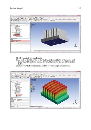
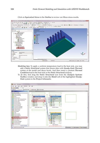
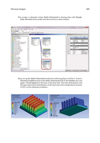
Thermal Analysis
9.2.2.2 2-D Cases
For plane stress, we have:
ε
ε
ε
γ
α
α
o
o
=










=










x
y
xy
T
T
∆
∆
0
(9.14)
For plane strain, we have:
ε
ε
ε
γ
ν α
ν α
o
o
=










=
+
+










x
y
xy
T
T
( )
( )
1
1
0
∆
∆ (9.15)
in which, ν is Poisson’s ratio.
9.2.2.3 3-D Case
ε
ε
ε
ε
γ
γ
γ
α
α
α
o
o
=






















=




x
y
z
xy
yz
zx
T
T
T
∆
∆
∆
0
0
0



















(9.16)
Observation: Temperature changes do not yield shear strains.
In both 2-D and 3-D cases, the total strain can be given by the following vector equation:
ε = εe + εo (9.17)
And the stress–strain relation is given by
σ = Eεe = E(ε − εo) (9.18)
9.2.2.4 Notes on FEA for Thermal Stress Analysis
Need to specify α for the structure and ΔT on the related elements (which experience the
temperature change).
• Note that for linear thermoelasticity, same temperature change will yield same
stresses, even if the structure is at two different temperature levels.
• Differences in the temperatures during the manufacturing and working environ-
ment are the main cause of thermal (residual) stresses.
A more comprehensive review of thermal problems, their governing equations and
boundary conditions can be found in the references, such as References [13,14].

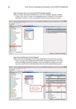
321. 306 Finite Element Modeling and Simulation with ANSYS Workbench
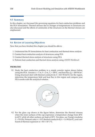
9.3 Modeling of Thermal Problems
Heat transfers in three ways through conduction, convection, and radiation. In FEM,
conduction is modeled by solving the resulting heat balance equations for the nodal
temperatures under specified thermal boundary conditions. Convection is modeled as a
surface load with a user-specified heat transfer coefficient and a given bulk temperature
of the surrounding fluid. Radiation effects, which are nonlinear, are typically modeled
by using the radiation link elements or surface effect elements with the radiation option.
Material properties such as density, thermal conductivity, and specific heat are needed
as input parameters for transient thermal analysis, while steady-state thermal analysis
needs only thermal conductivity as the material input. For thermal stress analysis, mate-
rial input parameters include Young’s modulus, Poisson’s ratio, and thermal expansion
coefficient. In the following, modeling of thermal problems is briefly illustrated with the
aid of two examples.
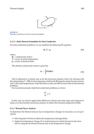
9.3.1 Thermal Analysis
First, we use a heat sink model taken from Reference [14] for thermal analysis. A heat sink
is a device commonly used to dissipate heat from a CPU in a computer. In this heat sink
model, a given temperature field (T = 120) is specified on the bottom surface and a heat flux
condition (Q k T n
≡ − = −
∂ ∂
/ 0 2
. ) is specified on all the other surfaces. An FE mesh with a
total node of 127,149 is created as shown in Figure 9.4. Using the steady-state thermal analy-
sis system in ANSYS, the computed temperature distribution on the heat sink is calculated
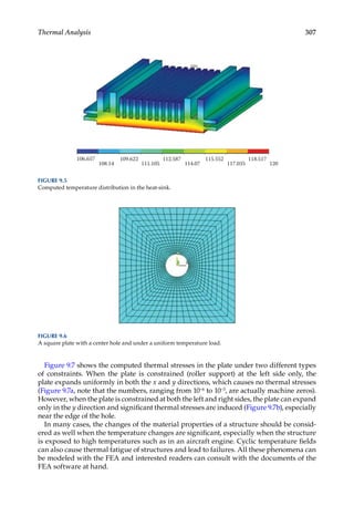
as shown in Figure 9.5. The cooling effect of the heat sink is most evident.
9.3.2 Thermal Stress Analysis
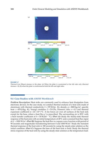
Next, we study the thermal stresses in structures due to temperature changes. For this
purpose, we employ the same model of a plate with a center hole (Figure 9.6) as used in
Chapters 4 and 5 to show the relation between the thermal stresses and constraints. We
assume that the plate is made of steel with Young’s modulus E = 200 GPa, Poisson’s ratio
ν = 0.3, and thermal expansion coefficient α = 12 × 10−6/°C. The plate is applied with a uni-
form temperature increase of 100°C.
FIGURE 9.4
A heat-sink model used for heat conduction analysis.

322. 307
Thermal Analysis
Figure 9.7 shows the computed thermal stresses in the plate under two different types
of constraints. When the plate is constrained (roller support) at the left side only, the
plate expands uniformly in both the x and y directions, which causes no thermal stresses
(Figure 9.7a, note that the numbers, ranging from 10−6 to 10−3, are actually machine zeros).
However, when the plate is constrained at both the left and right sides, the plate can expand
only in the y direction and significant thermal stresses are induced (Figure 9.7b), especially
near the edge of the hole.
In many cases, the changes of the material properties of a structure should be consid-
ered as well when the temperature changes are significant, especially when the structure
is exposed to high temperatures such as in an aircraft engine. Cyclic temperature fields
can also cause thermal fatigue of structures and lead to failures. All these phenomena can
be modeled with the FEA and interested readers can consult with the documents of the
FEA software at hand.
106.657
108.14
109.622
111.105
112.587
114.07
115.552
117.035
118.517
120
MN
FIGURE 9.5
Computed temperature distribution in the heat-sink.
FIGURE 9.6
A square plate with a center hole and under a uniform temperature load.

323. 308 Finite Element Modeling and Simulation with ANSYS Workbench
9.4 Case Studies with ANSYS Workbench
Problem Description: Heat sinks are commonly used to enhance heat dissipation from
electronic devices. In the case study, we conduct thermal analysis of a heat sink made of
aluminum with thermal conductivity k = 170 W/(m ⋅ K), density ρ = 2800 kg/m3, ­specific
heat c = 870 J/(kg ⋅ K), Young’s modulus E = 70 GPa, Poisson’s ratio ν = 0.3 and thermal
expansion coefficient α = 22 × 10−6/°C. A fan forces air over all surfaces of the heat sink
except for the base, where a heat flux q’ is prescribed. The surrounding air is 28°C with
a heat transfer coefficient of h = 30 W/(m2 ⋅ °C). (Part A): Study the steady-state thermal
response of the heat sink with an initial temperature of 28°C and a constant heat flux input
of q’ = 1000 W/m2. (Part B): Suppose the heat flux is a square wave function with period of
90 seconds and magnitudes transitioning between 0 and 1000 W/m2. Study the transient
thermal response of the heat sink in 180 seconds by using the steady-state solution as the
initial condition. (Part C): Suppose the base of the heat sink is fixed. Study the thermal
stress response of the heat sink by using the steady-state solution as the temperature load.
.681E-06 .584E-04 .156E-03 .258E-03 .352E-03
.456E-04 .147E-03 .245E-03 .343E-03 .441E-03
(a)
(b)
.259E+08 .169E+09 .313E+09 .456E+09 .600E+09
.576E+08 .241E+09 .354E+09 .528E+09 .671E+09
FIGURE 9.7
Thermal (von Mises) stresses in the plate: (a) When the plate is constrained at the left side only (thermal
stresses = 0); (b) when the plate is constrained at both the left and right sides.

324. 309
Thermal Analysis
Material: Aluminum
k = 170 W/(m · K)
ρ = 2800 kg/m3; c = 870 J/(kg · K)
E = 70 GPa; ν = 0.3
α = 22 × 10–6 1/°C
Boundary Conditions:
Air temperature of 28°C; h = 30 W/(m2 · °C).
Steady-state: q' = 1000 W/m2 on the base.
Transient: Square wave heat flux on the base.
Initial Conditions:
Steady-state: Uniform temperature of 28°C.
Transient: Steady-state temperature results.
Base of the
heat sink
All dimensions are in millimeters.
Part A: Steady-State Thermal Analysis
Step 1: Start an ANSYS Workbench Project
Launch ANSYS Workbench and save the blank project as ‘Heatsink.wbpj’.
Step 2: Create a Steady-State Thermal Analysis System
Drag the Steady-State Thermal icon from the Analysis Systems Toolbox
window and drop it inside the highlighted green rectangle in the Project
Schematic window.
Step 3: Add a New Material
Double-click on the Engineering Data cell to add a new material. In the follow-
ing Engineering Data interface which replaces the Project Schematic, type

325. 310 Finite Element Modeling and Simulation with ANSYS Workbench
‘Aluminum’ as the new material name, and double-click Isotropic Thermal
Conductivity under Thermal in the Toolbox window. Change the Unit to
‘Wm^-1K^-1’ and enter ‘170’ for Isotropic Thermal Conductivity in the
Properties window. Close the A2:Engineering Data tab to return to the
Project Schematic.
Step 4: Launch the SpaceClaim Program
Double-click the Geometry cell to launch SpaceClaim.

326. 311
Thermal Analysis
Step 5: Create a Profile Sketch
To customize units, select the SpaceClaim Options from the File menu. In the
SpaceClaim Options window that opens, click Units from the left naviga-
tion panel, and select Millimeters for Length. Next, change the Minor Grid
Spacing to 1mm. Click OK.

327. 312 Finite Element Modeling and Simulation with ANSYS Workbench
Right-click anywhere in the Graphics Window, and click Select New Sketch
Plane in the context menu.
Browse over to the x-y plane and click to highlight the x-y plane as shown below.

328. 313
Thermal Analysis
Click on the Plan View icon, and click the Line icon on the Design tab. Draw the
line sketch as shown below.
Click on the Mirror icon on the Design tab. In the Graphics Window, click on the
y-axis to set it as the mirror plane. Drag in the Graphics Window to create
a selection box around the line sketch. The selected lines will be mirrored as
shown below.

329. 314 Finite Element Modeling and Simulation with ANSYS Workbench
Step 6: Create an Extruded Body
Click the Pull icon on the Design tab. Pull the mirrored line sketch along the
z-axis. Enter 15mm in the textbox for Depth. A solid body will be created as
shown below.
Step 7: Launch the Steady-State Thermal Program
Double-click on the Model cell to launch the Steady-State Thermal program.
Click on the SYSSolid under Geometry in the Project Outline. In the Details
of “SYSSolid”, click to the right of the Material Assignment field and select
Aluminum from the drop-down menu.

330. 315
Thermal Analysis
Step 8: Generate Mesh
Right click on Mesh in the Project Outline. Select Insert and then Sizing from
the context menu. In the Details of “Sizing”, enter’5e-4 m’ for the Element
Size. Click on the Body icon in the toolbar to turn on the body selection filter.
Click on the solid body in the Graphics Window and apply it to the Geometry
selection.
Right-click on Mesh and select Generate Mesh.

331. 316 Finite Element Modeling and Simulation with ANSYS Workbench
Step 9: Apply Boundary Conditions
Right-click on Steady-State Thermal(A5). Choose Insert and then Heat Flux
from the context menu. Click the Face icon in the toolbar to turn on the face
selection filter. Apply a heat flux of 1000 W/m2 to the base of the heat sink.
Right-click on Steady-State Thermal(A5). Choose Insert and then Convection
from the context menu. In the Details of “Convection”, enter 30 W/(m2 ⋅ °C)
for Film Coefficient and 28°C for Ambient Temperature to all surfaces (a total
of 29 faces) except for the base of the heat sink.

332. 317
Thermal Analysis
Step 10: Solve and Retrieve Results
Right-click on Solution (A6) in the Outline, and insert Temperature, Total
Heat Flux, and Directional Heat Flux to the solution outline. In the Details
of “Directional Heat Flux”, set the Orientation to Y-axis. Right-click on
Solution (A6) and click Solve.
Click on Temperature in the Outline to review the temperature distribution.

333. 318 Finite Element Modeling and Simulation with ANSYS Workbench
Click on Total Heat Flux to display the heat flux with directional arrows.
Click on Directional Heat Flux to review the heat flux isolines along Y-axis.
Part B: Transient Thermal Analysis
Step 1: Add a Transient Thermal Analysis System
Drag the Transient Thermal icon from the Analysis Systems Toolbox window
and drop it onto the Solution cell of the highlighted Steady-State system in
the Project Schematic.

334. 319
Thermal Analysis
This creates a Transient Thermal system that shares data with Steady-State
Thermal system. The temperature distribution from the Steady-State Thermal
analysis is now the initial temperature for the Transient Thermal analysis. If
the initial temperature is uniform for the Transient Thermal analysis, then
this data sharing is not needed.

335. 320 Finite Element Modeling and Simulation with ANSYS Workbench
Step 2: Add Material Properties
Double-click on Engineering Data of Steady-State Thermal. Add a Density
of 2800 kg/m3, change the Unit to ‘JKg^-1K^-1’ and enter Specific Heat of
870 J/­(kg ⋅ K) to the Properties of Aluminum. Close the A2,B2:Engineering
Data interface.
Step 3: Set Up Transient Thermal Analysis
Double-click on the Setup cell of the Transient Thermal system to launch the
Multiple Systems–Mechanical program. Click Yes on the pop-up window to
read the modified upstream data.
Select Analysis Settings from the Project Outline. In the Details of “Analysis
Settings”, under Step Controls, set the Step End Time to 180s. Change the
Auto Time Stepping to On from Program Controlled. Change Defined By to
Time. The default values for the initial and the maximum time steps are small
for this model. Set the Initial Time Step to 0.1. Set the Minimum Time Step to
0.05. Set the Maximum Time Step to 5. A small time step will help increase the
accuracy of the model and also produce enough result steps so the animation
will have smooth transition between solution steps.

336. 321
Thermal Analysis
Step 4: Apply Cycling Heat Flux
Right-click on Transient Thermal (B5). Choose Insert and then Heat Flux from
the context menu. In the Details of “Heat Flux”, change Magnitude to Tabular
Data, and apply the heat flux to the bottom surface of the heat sink as shown
below.

337. 322 Finite Element Modeling and Simulation with ANSYS Workbench
Click on Tabular Data on the right edge of the Graphics window, and then click
on the push pin labeled AutoHide to display the Tabular Data window as
shown below. Enter the following values in the Tabular Data table.
Step 5: Apply Convective Boundary Condition
Right-click on Transient Thermal (B5). Choose Insert and then Convection from
the context menu. In the Details of “Convection”, enter 30 W/(m2 ⋅ °C) for
Film Coefficient and 28°C for Ambient Temperature to all surfaces (a total of
29 faces) except for the base of the heat sink.

338. 323
Thermal Analysis
Step 6: Solve and Retrieve Results
Right-click on Solution (B6) in the Outline, and insert Temperature, Total Heat
Flux, and Directional Heat Flux. In the Details of “Directional Heat Flux”,
set the Orientation to Y-axis. Right-click on Solution (B6) and click Solve.
Click on Temperature in the Outline to review the distribution. To show Graph,
click on Graph on the right side of the Graphics window, and then click on the
push pin labeled AutoHide.
Click on Total Heat Flux to display the heat flux with directional arrows.

339. 324 Finite Element Modeling and Simulation with ANSYS Workbench
Click on Directional Heat Flux to review the heat flux isolines along Y-axis.
Modeling tips: In the case study, an end time of 180 seconds is specified in the
transient setup. By default, the last set of results (solution at 180s) from the
transient analysis is used for graphics window display. To display results at
a different time point, e.g. temperature distribution at 40 seconds, you may
change the Display Time from Last to 40 s in the Details of “Temperature”.
Then right click on Solution (B6) and select Evaluate All Results. A result at
the specified time will be displayed at the Graphics Window as shown below.

340. 325
Thermal Analysis
Part C: Thermal Stress Analysis
Step 1: Add a Static Structural Analysis System
Drag the Static Structural icon from the Analysis Systems Toolbox window and
drop it onto the Solution cell of the highlighted Steady-State system in the
Project Schematic.
This creates a Static Structural system that shares data with Steady-State
Thermal system as shown below. The temperature distribution from the
Steady-State Thermal analysis is now the load input for the Static Structural
analysis. If a uniform temperature is specified as a load for the Static Structural
analysis, then data sharing of the steady-state thermal solution is not needed.

341. 326 Finite Element Modeling and Simulation with ANSYS Workbench
Step 2: Add Material Properties
Double-click Engineering Data of Steady-State Thermal. Add Young’s Modulus
of 70 GPa, Poisson’s ratio of 0.3 and Isotropic Instantaneous Coefficient of
Thermal Expansion of 2.2E-5 1/°C to the Properties of Aluminum as shown
below. Close the A2,B2,C2:Engineering Data interface.
Step 3: Set Up Static Structural Analysis
Double-click on the Setup cell of the Static Structural system to launch the
Multiple Systems–Mechanical program. Click Yes on the pop-up window to
read the modified upstream data.
Note an Imported Load item is automatically added to Static Structural (C5)
in the Outline tree. Right-click on Static Structural (C5) and insert a Fixed
Support to the Outline. Apply the fixed support to the bottom face of the heat
sink.

342. 327
Thermal Analysis
Step 4: Solve and Retrieve Results
Right-click on Solution (C6) in the Outline, and insert Total Deformation and
Equivalent Stress to the outline. Then right-click on Solution (C6) and click
Solve.
Click on Total Deformation in the Outline to review displacement results.

343. 328 Finite Element Modeling and Simulation with ANSYS Workbench
Click on Equivalent Stress in the Outline to review von Mises stress results.
Modeling tips: To apply a uniform temperature load to the heat sink, you may
add a Static Structural system that shares data with Steady-State Thermal
system at the model and above levels. And then insert a constant Thermal
Condition load to the heat sink in the Static Structural analysis.
To do this, first drag the Static Structural icon from the Analysis Systems
Toolbox window and drop it onto the Model cell of the highlighted Steady-
State system in the Project Schematic.

344. 329
Thermal Analysis
This creates a schematic where Static Structural is sharing data with Steady-
State Thermal at the model and above levels as shown below.
Next, set up the Static Structural analysis by following Step 3 of Part C. Insert a
Thermal Condition load to the Static Structural (C5) in the Outline tree and
apply a Fixed Support to the base of the heat sink. The total deformation and
the equivalent stress distributions of the heat sink with a temperature increase
of 10°C can be obtained as follows.

345. 330 Finite Element Modeling and Simulation with ANSYS Workbench
9.5 Summary
In this chapter, we discussed the governing equations for heat conduction problems and
the FEA formulation. Thermal stresses due to changes of temperatures in structures are
also discussed and the effects of constraints of the structures on the thermal stresses are
emphasized.
9.6 Review of Learning Objectives
Now that you have finished this chapter you should be able to
1. Understand the FE formulations for heat conduction and thermal stress analysis
2. Conduct heat conduction analysis of structures using FEA
3. Conduct thermal stress analysis of structures using FEA
4. Perform heat conduction and thermal stress analysis using ANSYS Workbench
PROBLEMS
9.1 Study the heat conduction problem in a simple annular region shown below,
using the FEA. Assume a = 1 m, b = 2 m, Ta = 100°C, and heat flux Qb = 200 W/m2.
Using structural steel with thermal conductivity k = 60.5 W/(m°C) for the region,
determine the temperature field and heat flux in this region and compare your
FEA results with the analytical solution.
a b
O
V
Sb
Sa
9.2 For the glass cup shown in the figure below, determine the thermal stresses
when the inner surfaces of the cup experience a temperature change from 20°C
to 60°C while all other surfaces are kept at 20°C. For glass, use Young’s modulus
E = 70 GPa, Poisson’s ratio ν = 0.17, thermal conductivity k = 1.4 W/(m°C), and coef-
ficient of thermal expansion α = 8.0 × 10−6/°C.

346. 331
Thermal Analysis
All dimensions are in millimeters.
40.000
100.000
4.000
30.000
26.000
4.000
9.3 Determine the temperature and heat flux distributions inside the following heat
transfer pipe with internal ribs. A bulk temperature of 80°C and 20°C with a film
coefficient of 100 W/(m2°C) and 30 W/(m2°C) is specified for the interior and exte-
rior convective heat transfer, respectively. Assume that the pipe is 30 cm long with
a thermal conductivity of 230 W/(m K) and that the two ends of the pipe are per-
fectly insulated.
All dimensions are in centimeters.
0.450
R5.500
0.450
2.500
2.500
0.450
2.500
0.450
2.500
R5.000
9.4 A 10 cm thick perforated concrete slab is shown below. The concrete has a
thermal conductivity k = 1.0 W/(m K), Young’s modulus E = 29 GPa, Poisson’s
ratio ν = 0.15, and thermal expansion coefficient α = 11 × 10−6/°C. The bulk tem-
perature of the fluid inside the circular perforated holes is 60°C with a film

347. 332 Finite Element Modeling and Simulation with ANSYS Workbench
coefficient of 100 W/(m2°C). Suppose the four sides of the concrete slab are kept
at a constant temperature of 20°C. The front and back faces of the perforated slab
are perfectly insulated. (1) Determine the temperature distribution in the slab.
(2) Find the thermally induced deformation and stresses in the slab if the four
sides are fixed.
All dimensions are in centimeters.
Front face
Side faces
D5.000 6.000
25.000
25.000
6.000
9.5 The following thermal bimorph is made of Silicon with a thermal conductivity
k = 130 W/(m°C), Young’s modulus E = 200 GPa, Poisson’s ratio ν = 0.27, and ther-
mal expansion coefficient α = 2.6 × 10−6/°C. It is 1 mm thick with fixed tempera-
tures of 60°C and 10°C, respectively, at the leftmost ends of its hot arm and cold
arm, as shown below. Suppose the bimorph has a uniform internal heat genera-
tion at 100 W/m3, and ignore the effects of convective heat transfer. (1) Determine
the steady-state temperature distribution in the thermal bimorph. (2) Determine
the thermally induced deformation and stresses in the bimorph if the two arms
are fixed on their left ends.
Hot arm
Cold arm
All dimensions are in millimeters.
Thot = 60°C
Tcold = 10°C
6.000 3.000
2.000
3.000
2.000
2.000
5.000
12.000
9.6 The heat sink shown below has a square base of size 22 mm × 22 mm × 2 mm
and consists of an array of square pin-fins, each of size 2 mm × 2 mm × 8 mm.
The pin-fins are separated by a gap distance of 4 mm in each direction. The heat

348. 333
Thermal Analysis
sink is initially at a temperature of 28°C. Suppose a heat flux input is prescribed
on the bottom face of the heat sink. The heat flux is of a symmetrical square wave
pattern with a period of 60 s (equal time for each half-cycle) and peak magni-
tudes transitioning from 800 W/m2 to 0 W/m2. A fan forces air over all surfaces
of the heat sink except for the bottom face, where the heat flux is prescribed. The
surrounding air is 28°C with a film coefficient of 30 W/(m2°C). Assume that the
heat sink is made of aluminum with thermal conductivity k = 170 W/(m K), den-
sity ρ = 2800 kg/m3, specific heat c = 870 J/(kg K), Young’s modulus E = 70 GPa,
Poisson’s ratio ν = 0.3, and thermal expansion coefficient α = 22 × 10−6/°C. Study
the transient thermal response of the heat sink during the first three cycles.
9.7 The electric kettle base shown below has a thickness of 0.5 cm and is made of struc-
tural steel with thermal conductivity k = 60.5 W/(m K), density ρ = 7850 kg/m3,
and specific heat c = 434 J/(kg K). Suppose a heat flux condition is defined through
a serpentine heating element embedded at the bottom of the kettle base. Except
for the imprinted heating element face, all other faces of the kettle base are sub-
jected to convective heat transfer with a bulk air temperature of 40°C and a film
coefficient of 80 W/(m2°C). (1) Study the steady-state thermal response of the
kettle base if a constant heat flux of 800 W/(m2°C) is applied through the heat-
ing element. (2) Suppose the heating element is cycled on and off with a period
of 60 s (30 s on-time followed by 30 s off-time). During on-time, the heat flux is
of magnitude 1000 W/(m2°C). Study the transient thermal response of the kettle
base for a period of 120 s using the steady-state solution as the initial condition.
Heating element is shown as
an imprinted face on the
bottom of the kettle base.
Isometric view of the two sides of the kettle base

349. 334 Finite Element Modeling and Simulation with ANSYS Workbench
All dimensions are in
centimeters.
0.500 2.000
1.500
R10.000
8.000
R1.250
10.000
2.000
1.000
R6.000
R1.500
9.8 The air to water heat exchanger shown below is made of copper with thermal
conductivity k = 400 W/(m K), Young’s modulus E = 100 GPa, Poisson’s ratio
ν = 0.3, and thermal expansion coefficient α = 18 × 10−6/°C. The exterior surfaces
are in contact with cold water with a film coefficient of 30 W/(m2°C) and a bulk
temperature of 20°C. The interior surfaces are in contact with hot air with a film
coefficient of 100 W/(m2°C) and a bulk temperature of 80°C. (1) Determine the
steady-state thermal response of the heat exchanger. (2) Suppose the two annulus
faces at the ends of the heat exchanger are fixed. Determine the thermal deforma-
tion and stresses induced in the exchanger.
All dimensions are in millimeters.
R10.000
20.000
R10.000
40.000 20.000
R5.000
R3.000
10.000
9.9 Thermal expansion mismatch is of great concern in high-density semiconductor
devices. The model shown below consists of a copper dye on a silicon substrate.
Suppose the dye and substrate are perfectly bounded and the substrate is fixed
on the bottom face. Determine the thermally induced deformation and stresses if
the dye is assigned a uniform temperature of 60°C and the substrate is assigned
a uniform temperature of 40°C. For copper, use Young’s modulus E = 100 GPa,
Poisson’s ratio ν = 0.3, and thermal expansion coefficient α = 18 × 10−6/°C, and for
silicon, use E = 200 GPa, ν = 0.27, and α = 2.6 × 10−6/°C.

350. 335
Thermal Analysis
All dimensions are in millimeters.
Die thickness = 2 mm
Substrate thickness = 2 mm
Copper die
Silicon substrate
40.000
20.000
20.000
40.000
9.10 The following square platform with two arms has a thickness of 1 mm and is
made of silicon with a thermal conductivity k = 130 W/(m°C), Young’s modu-
lus E = 200 GPa, Poisson’s ratio ν = 0.27, and thermal expansion coefficient
α = 2.6 × 10−6/°C. Ignore the effects of convective heat transfer. (1) Determine the
temperature distribution in the platform when the temperatures of the upper
and lower ends are set uniform at 40°C and 20°C, respectively, as shown below.
(2) Suppose the ends of the two arms are fixed. Determine the thermally induced
deformation and stresses in the platform.
All dimensions are in centimeters.
Tupper = 40°C
Tlower = 20°C
1.000 12.000
1.000
1.000
10.000
1.000
1.000
10.000
12.000 1.000

352. 337
10
Introduction to Fluid Analysis
10.1 Introduction
Flow simulations are widely used in engineering applications ranging from flow around
airplane wings and hydraulic turbines to flow in blood vessels and other circulatory sys-
tems (see Figure 10.1). We may gain a better understanding of the motion of fluid around
objects as well as the fluid behavior in complex circulatory systems by conducting fluid
analysis. Computational fluid dynamics (CFD) simulation complements experimental test-
ing, helps reduce cost and turnaround time for design iterations, and has become an indis-
pensable tool whenever practical design involving fluids is required. In this chapter, we
will discuss fluid analysis using ANSYS® Workbench.
10.2 Review of Basic Equations
We begin by briefly reviewing the fundamentals of fluid mechanics.
10.2.1 Describing Fluid Motion
In fluid dynamics, the motion of a fluid is mathematically described using physical quanti-
ties such as the flow velocity u, flow pressure p, fluid density ρ, and fluid viscosity ν. The
flow velocity or flow pressure is different at a different point in a fluid volume. The objec-
tive of fluid simulation is to track the fluid velocity and pressure variations at different
points in the fluid domain.
10.2.2 Types of Fluid Flow
There are many different types of fluid flow. A flow can be compressible (ρ ≠ constant)
or incompressible (ρ = constant), viscous (ν ≠ 0) or inviscid (ν = 0), steady ( )
∂ ∂
u/ t = 0 or
unsteady ( )
∂ ∂
u/ t ≠ 0 and laminar (streamline) or turbulent (chaotic). Furthermore, a fluid
can be Newtonian (if the viscosity depends only on temperature and pressure, not on
forces acting upon it; in other words, shear stress is a linear function of the fluid strain rate)
or non-Newtonian (if the viscosity depends on forces acting upon it, i.e., shear stress is a
nonlinear function of the fluid strain rate).

353. 338 Finite Element Modeling and Simulation with ANSYS Workbench
10.2.3 Navier–Stokes Equations
For the purpose of this chapter, we limit ourselves to the study of incompressible
Newtonian flows. All fluids are compressible to some extent, but we may consider most
common liquids as incompressible, whose motion is governed by the following Navier–
Stokes (N–S) equations:
∂
∂ ρ
u
u u u f
t
p
= − ∇ + ∇ −
∇
+
ν 2
(10.1)
which shows that the acceleration ∂ ∂
u/ t of a fluid particle can be determined by the com-
bined effects of advection u u
∇ , diffusion ν∇2
u, pressure gradient ∇p/ρ, and body force f.
The N–S equations can be derived directly from the conservation of mass, momentum,
and energy principles. Note that for each particle of a fluid field we have a set of N–S
equations. A particle’s change in velocity is influenced by how the surrounding particles
are pushing it around, how the surrounding resists its motion, how the pressure gradient
changes, and how the external forces such as gravity act on it [15].
In 3-D Cartesian coordinates, the N–S equations become:
ρ
∂
∂
∂
∂
∂
∂
∂
∂
ν
∂
∂
∂
∂
∂
∂
u
t
u
u
x
v
u
y
w
u
z
u
x
u
y
u
z
+ + +





 = + +





 −
2
2
2
2
2
2
∂
∂
∂
p
x
fx
+ (10.2)
ρ
∂
∂
∂
∂
∂
∂
∂
∂
ν
∂
∂
∂
∂
∂
∂
v
t
u
v
x
v
v
y
w
v
z
v
x
v
y
v
z
+ + +





 = + +





 −
2
2
2
2
2
2
∂
∂
∂
p
y
fy
+ (10.3)
ρ
∂
∂
∂
∂
∂
∂
∂
∂
ν
∂
∂
∂
∂
∂
∂
w
t
u
w
x
v
w
y
w
w
z
w
x
w
y
w
z
+ + +





 = + +





 −
2
2
2
2
2
2
∂
∂
∂
p
z
fz
+ (10.4)
where u, v, and w are components of the particle’s velocity vector u.
In CFD modeling, the N–S equations for particle motion are numerically solved, along
with specified boundary conditions, on a 3-D grid that represents the fluid domain to be
FIGURE 10.1
Examples of CFD: (a) airflow around a tractor (Courtesy ANSYS, Inc., http://www.ansys.com/Industries/
Automotive/Application+Highlights/Body), and (b) streamlines inside a combustion chamber (Courtesy
ANSYS, Inc., http://www.edr.no/en/courses/ansys_cfd_advanced_modeling_ reacting_flows_and_combus-
tion_in_ans ys_fluent).

354. 339
Introduction to Fluid Analysis
analyzed. For more details on numerical solution techniques adopted in CFD, please refer
to the theory guide in ANSYS online documentation.
10.3 Modeling of Fluid Flow
Practical aspects of CFD modeling are discussed next. The topics include fluid domain
specification, meshing, boundary condition assignments, and solution visualization.
10.3.1 Fluid Domain
A fluid domain is a continuous region with respect to the fluid’s velocity, pressure, density,
viscosity, and so on. Figure 10.2 illustrates examples of an internal flow and an external
flow. For an internal flow (see Figure 10.2a), the fluid domain is confined by the wetted
surfaces of the structure in contact with the fluid. For an external flow (see Figure 10.2b),
the fluid domain is the external fluid region around the immersed structure.
10.3.2 Meshing
In CFD analysis, mesh quality has a significant impact on the solution time and accuracy
as well as the rate of convergence. A good mesh needs to be fine enough to capture all rel-
evant flow features, such as the boundary layer and shear layer and so on (see Figure 10.3),
without overwhelming the computing resources. A good mesh should also have smooth
and gradual transitions between areas of different mesh density, to avoid adverse effect on
convergence and accuracy.
10.3.3 Boundary Conditions
Appropriate boundary conditions are required to fully define the flow simulation, as the
flow equations are solved subject to boundary conditions. The common fluid boundary
conditions include the inlet, outlet, opening, wall, and symmetry plane [16]. An inlet con-
dition is used for boundaries where the flow enters the domain. An outlet condition is for
where the flow leaves the domain. An opening condition is used for boundaries where the
fluid can enter or leave the domain freely. A wall condition represents a solid boundary of
External flow
Internal flow
(a) (b)
FIGURE 10.2
Flow region definition: (a) internal flow and (b) external flow.

355. 340 Finite Element Modeling and Simulation with ANSYS Workbench
the flow model. For fixed walls, this typically means a no-slip boundary condition for the
flow velocity. A symmetry plane condition is used for planes exhibiting both geometric
and flow symmetry.
A pressure boundary is a boundary where the flow pressure is defined. A velocity
boundary is a boundary where the velocity profile is given. Figure 10.4 gives two simu-
lated airflow streamline plots for a city block. The boundary conditions for (a) include a
velocity inlet on the left edge, a pressure outlet on the right edge, and wall conditions on all
buildings (depicted in gray lines). The boundary conditions for (b) include pressure inlets
on the four sides of the city block, a pressure outlet at the city’s circular center, and wall
conditions on all buildings. As we can see from Figure 10.4, different boundary conditions
result in different flow patterns. Assigning realistic boundary conditions that truly reflect
the flow conditions is crucial in CFD analysis.
10.3.4 Solution Visualization
Once a problem is setup with the fluid domain meshed and the boundary conditions spec-
ified, it can be submitted to the solver for computation of a solution. Flow motion can be
described by plotting the flow variables on a section plane or in 3-D space. The commonly
used plots in CFD are contour plots of pressure, shear strain rate and turbulence kinetic
Flow Inadequate mesh Better mesh
FIGURE 10.3
The resolution of a mesh needs to adequately represent the flow feature.
0 5.00e+004 1.00e+005 (m) 0 5.00e+004 1.00e+005 (m)
(a) (b)
FIGURE 10.4
Airflow over a city block: (a) crosswind blowing from left to right; (b) a circular low-pressure area at the city center.

356. 341
Introduction to Fluid Analysis
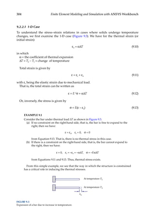
energy distributions, streamline plot, and vector plot of velocity field. Figure 10.5 shows
the related solution plots of a flow passing over a single cylinder. A symmetric half-model
is used in the example, with the flow pressure, velocity, shear stress, turbulence intensity,
and particle trajectories plotted as shown above.
10.4 Case Studies with ANSYS Workbench
Problem Description: The aerodynamic performance of vehicles can be improved by
utilizing computational fluid dynamics simulation. In this case study, we conduct fluid
Turbulence kinetic energy
Contour 2
Velocity
Streamline 1
Contour 1
Pressure
3.820e-005
(a) (b)
(c) (d)
7.329e-002
6.600e-002
6.714e-006 7.669e-003
5.763e-003
3.858e-003
1.952e-003
4.635e-005
6.052e-006
5.390e-006
4.728e-006
4.066e-006
3.404e-006
2.742e-006
2.080e-006
1.418e-006
7.558e-007
9.375e-008
5.871e-002
5.142e-002
4.412e-002
3.683e-002
2.954e-002
2.225e-002
7.661e-003
3.685e-004
1.495e-002
3.105e-005
2.390e-005
1.674e-005
9.590e-006
2.438e-006
–4.715e-006
–1.187e-005
–1.902e-005
–2.617e-005
–3.333e-005
[Pa]
[mˆ2 sˆ–2]
[sˆ–1]
[msˆ–1]
Shear strain rate
Contour 1
Velocity
Vector 1
(e)
[msˆ–1]
7.669e-003
5.752e-003
3.835e-003
1.917e-003
0.000e-000
FIGURE 10.5
Solution plots of fluid flow past a single cylinder (a half-model using symmetry). (a) Pressure distribution; (b)
shear strain rate distribution; (c) turbulence kinetic energy distribution; (d) streamline; and (e) velocity vector
plot.

357. 342 Finite Element Modeling and Simulation with ANSYS Workbench
analysis of the air flow passing through a truck. Assume air at room temperature of 25°C
for the flow field with an air velocity of 40 km/hr blowing from left to right. Use non-slip
boundary conditions along the walls of the truck and the ground surface. Find the airflow
pattern as well as the pressure and velocity distributions of the flow field around the truck.
R0.200
1.200
3.000
2.000
R0.400
2.400
All dimensions are in meters. The truck body
is 1.6 m wide, and each wheel is 0.2 m wide.
R0.400
0.800
1.200
R0.500
Flow field: Incompressible air at 25°C.
Boundary conditions: Air is blowing from left to right at a velocity of 40 km/h.
Nonslip boundaries along the walls of the truck and the ground surface.
Step 1: Start an ANSYS Workbench Project
Launch ANSYS Workbench and save the blank project as ‘CFD_Truck.wbpj’.
Step 2: Create a Fluid Flow (CFX) Analysis System
Drag the Fluid Flow (CFX) icon from the Analysis Systems Toolbox window and
drop it inside the highlighted green rectangle in the Project Schematic window.

358. 343
Introduction to Fluid Analysis
Step 3: Launch the SpaceClaim Program
Double-click the Geometry cell to launch SpaceClaim.
Step 4: Create a Truck Model
Right-click anywhere on the Graphics Window, and click Select New Sketch
Plane from the context menu.

359. 344 Finite Element Modeling and Simulation with ANSYS Workbench
Mouse over x-y plane, and click to select the highlighted x-y plane. This will
change the sketch plane from the default x-z plane (shown above) to the x-y
plane (shown below).
Click Plan View on the toolbar to view the sketch grid head-on. Click Sketch
Mode on the Design tab to begin a sketch. Click on the Rectangle icon. Draw
two rectangles as shown below.

360. 345
Introduction to Fluid Analysis
Click the Create Rounded Corner icon on the Design tab. Draw two rounded
corners as shown below.
Click on the Pull icon on the Design tab. In the Graphics Window, ctrl-click the
two rectangular surfaces, and pull them along z-axis. Enter 0.8m in the box for
extrusion depth to create a solid. Press Esc to cancel the pull.
In the Graphics Window, click on the side face (with a surface normal pointing
along z-axis as shown below), and click the Sketch Mode icon on the Design
tab to start a new sketch on this face. Click on the Point icon.

361. 346 Finite Element Modeling and Simulation with ANSYS Workbench
In the lower left Options-Sketch panel, uncheck Snape to grid and Snap to angle,
and click Cartesian dimensions. Cartesian dimensions show you the x and y
distances from the point you select. In the Graphics Window, click the lower
left corner (labelled Point C in the figure below) to select it as the base point
and drag along line CA to create point A, enter 0.8m in the box for distance
between A and C. Next, use point A as the base point, and drag along line AB
to create point B, enter 2.4m in the box for distance between A and B.
Next, click the Sweep Arc icon on the Design tab, and create two half circles of
radius 0.4m centered at points A and B, respectively, as shown below.

362. 347
Introduction to Fluid Analysis
Click Pull on the Design tab. In the left Options-Pull panel, click No Merge and
Pull Both Sides, as well as Thicken surfaces. In the Graphics Window, Ctrl-
click the two half-circular surfaces (highlighted in orange), and pull them
along z-axis and enter 0.1m in the box for depth. This will create two additional
Solids in Structure Tree. Each Solid represents half of a wheel. The wheel
width is actually 0.2m because the pull is bi-directional with 0.1m on each side.
Click Mirror on the Design tab. In the Graphics Window, click the bottom face
of the truck to set it as the mirror plane, and Ctrl-click the two half-wheels to
mirror the geometry as follows.

363. 348 Finite Element Modeling and Simulation with ANSYS Workbench
In the Graphics Window, click on the Select Mirror Plane icon. Click on the back
side of the truck (with a normal pointing along negative z-axis) to set it as the
mirror plane (highlighted in purple below). Then, Ctrl-click the two wheels
and the truck body to mirror the geometry as follows. This will result in a total
of 5 Solid items (1 truck and 4 wheels) in the Structure Tree.
Click on the Select icon on the Design tab. Ctrl-click the 5 Solid items in the
Structure Tree to highlight them in yellow.

364. 349
Introduction to Fluid Analysis
Click on the Combine icon to merge them into a single Solid.
Step 5: Create a Box Enclosure
Click on the Enclosure icon on the Prepare tab. In the lower left Options-Enclosure
panel, select Box for the Enclosure type, and uncheck Symmetric dimensions.
In the Graphics Window, enter the cushion dimensions as shown below (3m
for cushion value along +x/ − x, 1m for cushion value along +z/ − z, 1.5m for
cushion value along +y, 1e-6m for cushion value along –y). Note that cushion
dimensions only accept non-zero values, although a small value of 1e-6m may
be displayed as 0 in the dimension box as shown below.

365. 350 Finite Element Modeling and Simulation with ANSYS Workbench
Click the Checkmark icon in the Graphics Window to create the enclosure. Now
an Enclosure item is added to the Structure Tree.
Right-click on the Solid item in the Structure Tree, and click Suppress for Physics
in the context menu. When suppressed, the Solid truck model will be excluded
for physical analysis, and only the Enclosure model will be used for subse-
quent CFD analysis. Exit the SpaceClaim.

366. 351
Introduction to Fluid Analysis
Step 6: Generate Mesh
Double-click on the Mesh cell to launch the Meshing program.
Click the EnclosureEnclosure item under Geometry in the Project Outline. In
the Details of “EnclosureEnclosure”, select Fluid for the Fluid/Solid field
under Materials.

367. 352 Finite Element Modeling and Simulation with ANSYS Workbench
Click on Mesh in the Outline. In the Details of “Mesh”, set the Relevance Center
to Medium under Sizing. Right click on Mesh in the Outline, and select
Update in the context menu to generate the mesh. After that, close the Fluid
Flow (CFX)-Meshing program.
Step 7: Set Up Flow Domain
Double-click on the Setup cell to launch the Fluid Flow (CFX) – CFX-Pre program.

368. 353
Introduction to Fluid Analysis
Double-click on Analysis Type in the Outline tree.
In the Details of Analysis Type in Flow Analysis 1, set the Analysis Type to
Steady State. Click Ok to exit the menu.

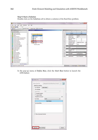
369. 354 Finite Element Modeling and Simulation with ANSYS Workbench
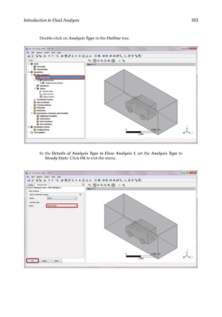
Next, double-click on Default Domain in the Outline tree.
In the Details of Default Domain in Flow Analysis 1, set the Domain Type to
Fluid Domain, Material to Air at 25C, and Reference Pressure to 1[atm].
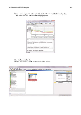
Click Ok to exit the menu.

370. 355
Introduction to Fluid Analysis
Step 8: Set Up Boundary Conditions
Add Inlet – Right-click on Default Domain in the Outline. Select Insert and then
Boundary.
Change the Name to Inlet in the pop-up menu shown below. Click Ok.

371. 356 Finite Element Modeling and Simulation with ANSYS Workbench
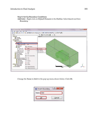
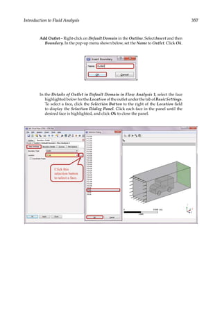
In the Details of Inlet in Default Domain in Flow Analysis 1, select the face
highlighted below for the Location of the inlet under the tab of Basic Settings.
To select a face, click the Selection Button to the right of the Location field
to display the Selection Dialog Panel. Click each face in the panel until the
desired face is highlighted, and click Ok to close the panel.
Click on the Boundary Details tab, and set the Normal Speed to 40 [Km Hr^-1].
Click OK.

372. 357
Introduction to Fluid Analysis
Add Outlet – Right-click on Default Domain in the Outline. Select Insert and then
Boundary. In the pop-up menu shown below, set the Name to Outlet. Click Ok.
In the Details of Outlet in Default Domain in Flow Analysis 1, select the face
highlighted below for the Location of the outlet under the tab of Basic Settings.
To select a face, click the Selection Button to the right of the Location field
to display the Selection Dialog Panel. Click each face in the panel until the
desired face is highlighted, and click Ok to close the panel.

373. 358 Finite Element Modeling and Simulation with ANSYS Workbench
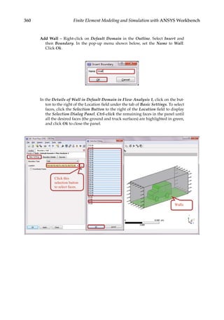
Click on the Boundary Details tab, and set the Relative Pressure to 0 [Pa]. Click
OK.
Add Opening – Right-click on Default Domain in the Outline. Select Insert and
then Boundary. In the pop-up menu shown below, set the Name to Opening.
Click Ok.

374. 359
Introduction to Fluid Analysis
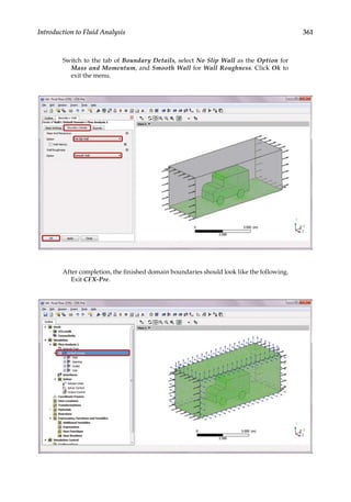
In the Details of Opening in Default Domain in Flow Analysis 1, click on the
button to the right of the Location field under the tab of Basic Settings. To
select faces, click the Selection Button to the right of the Location field to dis-
play the Selection Dialog Panel. Ctrl-click to highlight the 3 faces (top, left,
right side of the enclosure) in the panel, and click Ok to close the panel.
Switch to the tab of Boundary Details, set the Relative Pressure to 0 [Pa]. Click
Ok to exit.

375. 360 Finite Element Modeling and Simulation with ANSYS Workbench
Add Wall – Right-click on Default Domain in the Outline. Select Insert and
then Boundary. In the pop-up menu shown below, set the Name to Wall.
Click Ok.
In the Details of Wall in Default Domain in Flow Analysis 1, click on the but-
ton to the right of the Location field under the tab of Basic Settings. To select
faces, click the Selection Button to the right of the Location field to display
the Selection Dialog Panel. Ctrl-click the remaining faces in the panel until
all the desired faces (the ground and truck surfaces) are highlighted in green,
and click Ok to close the panel.

376. 361
Introduction to Fluid Analysis
Switch to the tab of Boundary Details, select No Slip Wall as the Option for
Mass and Momentum, and Smooth Wall for Wall Roughness. Click Ok to
exit the menu.
After completion, the finished domain boundaries should look like the following.
Exit CFX-Pre.

377. 362 Finite Element Modeling and Simulation with ANSYS Workbench
Step 9: Start a Solution
Double-click on the Solution cell to obtain a solution of the fluid flow problem.
In the pop-up menu of Define Run, click the Start Run button to launch the
CFX-Solver.

378. 363
Introduction to Fluid Analysis
When a menu pops up to indicate that the Solver Run has finished normally, click
Ok. Then exit the CFX-Solver Manager program.
Step 10: Retrieve Results
Double-click on the Results cell to visualize the results.

379. 364 Finite Element Modeling and Simulation with ANSYS Workbench
Plot Velocity Vector – Right-click User Locations and Plots in the Outline, and
select Insert and then Vector. Accept the default name Vector 1 in the pop-up
menu. In the Details of Vector 1, select All Domains for Domains, Default
Domain for Locations and Velocity for Variable, and click Apply. Check
Default Legend View 1 in the Outline to display the legend.
Plot Wall Pressure Contour – Right-click User Locations and Plots in the
Outline, and select Insert and then Contour. Accept the default name Contour
1 in the pop-up menu. In the Details of Contour 1, select All Domains for
Domains, Wall for Locations and Pressure for Variable, and click Apply.
Check Default Legend View 1 and Contour1, and uncheck Vector1 in the
Outline to view the pressure distribution on the wall.

380. 365
Introduction to Fluid Analysis
Plot Streamline – Right-click User Locations and Plots in the Outline, and
select Insert and then Streamline. Accept the default name Streamline 1 in
the pop-up menu. In the Details of Streamline 1, select 3D Streamline for
Definition, All Domains for Domains, Inlet for Start From, 150 for # of
Points, and Velocity for Variable, and click Apply. Check Default Legend
View 1, Streamline 1 and Wireframe, and uncheck Contour1 in the Outline
to view streamlines.

381. 366 Finite Element Modeling and Simulation with ANSYS Workbench
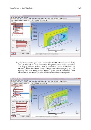
Modeling tips: Follow the steps below to visualize flow results on a section
plane. First, right-click User Locations and Plots in the Outline, then select
Insert and Location and then Plane in the context menu. Accept the default
name Plane 1 in the pop-up menu. In the Details of Plane 1, select All
Domains for Domains, XY Plane for Method and 0.0 [m] for Z, and click
Apply. Check Plane 1 and Wireframe in the Outline to view the created
section plane.
To generate a contour plot on the plane, right-click User Locations and Plots,
and select Insert and then Contour. Accept the default name Contour 2 in the
pop-up menu. In the Details of Contour 2, select All Domains for Domains,
Plane 1 for Locations and Velocity for Variable, and click Apply. Check
Default Legend View 1, Contour 2 and Wireframe in the Outline to retrieve
the velocity distribution on the section plane.

382. 367
Introduction to Fluid Analysis
To generate a streamline plot on the plane, right-click User Locations and Plots,
and select Insert and then Streamline. Accept the default name Streamline
2 in the pop-up menu. In the Details of Streamline 2, select All Domains for
Domains, Plane 1 for Start From, Rectangular Grid for Sampling, 0.03 for
Spacing, and click Apply. Check Default Legend View 1, Streamline 2 and
Wireframe in the Outline to view the streamlines on the section plane.

383. 368 Finite Element Modeling and Simulation with ANSYS Workbench
10.5 Summary
In this chapter, we briefly discussed the governing equations in fluid dynamics, main
variables of concern, boundary conditions, and procedures in conducting CFD model-
ing and analysis. A case study using ANSYS Workbench is demonstrated using a truck
model.
10.6 Review of Learning Objectives
Now that you have finished this chapter you should be able to
1. Understand the unique nature of fluid dynamics problems, including its govern-
ing equations, variables, and boundary conditions
2. Know how to create quality mesh for CFD analysis
3. Know how to apply the boundary conditions for CFD analysis
4. Perform CFD modeling and analysis of flows in complex domains using ANSYS
Workbench
PROBLEMS
10.1 Conduct fluid analysis of the water flow passing through a U-tube. The tube has
an inner and outer diameter of 4 and 4.2 cm, respectively. Assume nonslip bound-
ary conditions on the surface walls. The inlet flow velocity is 5 mm/s and the
outlet flow velocity is 4 mm/s. Determine the pressure and velocity distributions
of the interior flow field.
All dimensions are in centimeters.
R5.000
10.000
10.000
Outlet
Inlet

384. 369
Introduction to Fluid Analysis
10.2 Determine the pressure and velocity distributions of the flow of air over a solid
half-cylinder. The 20 cm long half-cylinder has a radius of 5 cm, and is placed on the
ground. The upstream air has a velocity of 5 mm/s, and the air in the downstream
passageway is at atmospheric pressure. Assume nonslip boundary conditions at the
air–solid interface and the air is at a constant room temperature of 25°C.
All dimensions are in
centimeters.
R5.000
Flow direction
10.3 Determine the pressure and velocity distributions of the flow of air over a solid
sphere. The sphere has a radius of 5 cm. The upstream air has a velocity of 5 mm/s,
and the air in the downstream passageway is at atmospheric pressure. Assume
nonslip boundary conditions at the spherical surface and the air is at a constant
room temperature of 25°C.
R5.000
All dimensions are in
centimeters.
Flow direction
10.4 The heat sink shown below has a square base of size 22 mm × 22 mm × 2 mm and
consists of an array of square pin-fins, each of size 2 mm × 2 mm × 8 mm. The
pin-fins are separated by a gap distance of 4 mm in each direction. Determine the
pressure and velocity distributions of the flow of air over the heat sink at room
temperature of 25°C. Suppose the square base of the heat sink is in contact with

385. 370 Finite Element Modeling and Simulation with ANSYS Workbench
the ground. The upstream air has a velocity of 10 mm/s, and the air in the down-
stream passageway is at atmospheric pressure.
Flow direction
10.5 Conduct fluid analysis of the air flow passing through an S-pipe. Assume nonslip
boundary conditions along the pipe walls and the air is at a room temperature of
25°C. The velocity of the air is 5 mm/s at the inlet and the outlet is at atmospheric
pressure. Determine the pressure and velocity distributions of the interior flow field.
All dimensions are in millimeters.
Inlet
R10.000
20.000
R5.000
R3.000
R10.000
20.000
10.000
Outlet
40.000
10.6 Conduct fluid analysis of the water flow passing through an orifice. Assume
nonslip boundary conditions on the walls. The water has a uniform velocity of
15 mm/s at the inlet and the outlet is at atmospheric pressure. Determine the
pressure and velocity distributions of the flow field.
All dimensions are in centimeters.
10.000
10.000
1.000
6.000
Inlet
Outlet

386. 371
Introduction to Fluid Analysis
10.7 Conduct fluid analysis of the water flow passing through a diffuser pipe. Assume
nonslip boundary conditions along the walls. The water has a uniform velocity
of 10 mm/s at the inlet and the outlet is at atmospheric pressure. Determine the
pressure and velocity distributions of the flow field.
All dimensions are in centimeters.
6.000 10.000
3.000
6.000
Outlet
Inlet
10.8 Conduct fluid analysis of the water flow passing through a transition pipe. Assume
nonslip boundary conditions along the walls. The water has a uniform velocity
of 25 mm/s at the inlet and the outlet is at atmospheric pressure. Determine the
pressure and velocity distributions of the flow field.
All dimensions are in centimeters.
8.000 8.000 8.000
3.000
Outlet
Inlet
5.000
10.9 Determine the pressure and velocity distributions of the flow of water inside the
following circular chamber. The chamber has a depth of 2 m. Assume nonslip
boundary conditions at the walls. The velocity of water at the inlets is 10 cm/s,
and the outlets are at atmospheric pressure.

387. 372 Finite Element Modeling and Simulation with ANSYS Workbench
All dimensions are in meters.
Inlet Inlet
Outlet
2.000
2.000
2.000
2.000
2.000
2.000
R1.500
2.000
2.000
R4.000
Outlet
10.10 Determine the pressure and velocity distributions of the flow of water inside the
following circular chamber. The chamber has a depth of 5 mm. Assume nonslip
boundary conditions at the walls. The velocity of water at the inlets is 5 mm/s,
and the outlets are at atmospheric pressure.
All dimensions are in millimeters.
Inlet
4.000 4.000
4.000
Outlet
Outlet
Inlet
4.000
4.000
4.000
4.000
4.000
R25.000
R12.000
R15.000
45.00°
45.00°
D10.000
45.00°
45.00°

388. 373
11
Design Optimization
11.1 Introduction
Optimization is an integral part of engineering design. Traditionally, optimization tasks
have been carried out mostly by trial and error, when unexpected failure of a design to
meet certain criteria is identified. Often, a best design is not obtained after many design
iterations. Only a feasible design meeting all the requirements is created. The conven-
tional way of changing a design when it is found to be deficient in certain criteria can be
incredibly costly and time-consuming. For today’s engineers, a more productive and cost-
effective practice is to use numerical optimization techniques to guide in the evaluation
of design trade-offs. Often, a best design is put forward after running simulation-based
optimization a few times. In this chapter, we will cover materials relating to the topics of
design optimization via simulation. The concepts of topology optimization, parametric
optimization, and design space exploration will be introduced, along with optimization
examples using ANSYS® Workbench.
11.2 Topology Optimization
A design’s performance should be optimized from different perspectives as the design
process evolves. In the early stage of a design, topology optimization can be used to help
designers arrive at a good initial design concept. The goal of topology optimization is to
find the ideal distribution of material within a predefined design space for a given set of
loading and boundary conditions. The regions that contribute the least to the load bear-
ing are identified and taken out from the design to minimize the weight. As a result, an
optimal material layout is determined, from which a good design concept can be derived.
Figure 11.1 illustrates topology optimization of a bridge structure. The 3-D design space
of the bridge is shown as a solid rectangle box in Figure 11.1a. The bridge is fixed on the
bottom two edges and applied a surface load on the top face. In Figure 11.1b, an arch is
clearly suggested as the ideal layout by the topology optimization study aiming at 80%
weight reduction. Materials are removed from the least stressed regions in the simulation
model, that is, regions contributing the least to the overall stiffnesss of the structure. This
optimization study perhaps helps elucidate why the arch continues to play an important
part in bridge design after thousands of years of architectural use.

389. 374 Finite Element Modeling and Simulation with ANSYS Workbench
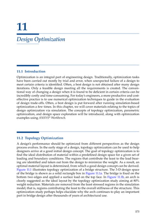
11.3 Parametric Optimization
In the final design stage, a design’s performance is greatly influenced by its shape and size.
Parametric optimization can be used to help designers determine the optimal shape and
dimensions of a structure. In parametric optimization, the independent variables whose
values can be changed to improve a design are called design variables. Design variables are
usually geometric parameters such as length, thickness, or control point coordinates that
control a design’s shape. Responses of the design to applied loads are known as state vari-
ables, which are functions of the design variables. Examples of state variables are stresses,
deformations, temperatures, frequencies, and so on. The restrictions placed on the design
are design constraints. In general, parametric optimization involves minimizing an objec-
tive function of the design variables subject to a given set of design constraints [17].
For example, consider the parametric optimization of a stiffened aluminum panel with
clamped edges. Stiffened panels are suited for weight-sensitive designs and are widely
used in ship decks, air vehicles, and offshore structures. The main drawback is that they
are light-weight structures with low natural frequencies, leading to a greater risk of reso-
nance. For the design shown in Figure 11.2, the variables that are allowed to change, that
is, the design variables, are the stiffener height h, the plate thickness t, the longitudinal
stiffener thickness tlong, and the lateral stiffener thickness tlat. To reduce the panel’s vulner-
ability to vibration-induced movement, its fundamental frequency fbase, that is, the state
variable in the study, is to be set above, say, 20 Hz. Suppose your objective is to minimize
the panel’s overall weight. You may set up a parametric optimization study solving for the
optimum values of the four design variables so as to minimize the panel’s weight while
satisfying the design constraint of fbase 20 Hz.
11.4 Design Space Exploration for Parametric Optimization
A “black box” model shown in Figure 11.3 can be used to illustrate the parametric optimi-
zation schematic, as a direct relationship between the design variables and responses is
generally unknown. The schematic includes the use of a parametric finite element model
for finding the effects of design variables (inputs) to the responses (outputs). After multiple
response datasets are collected from finite element simulations, a mapping relationship can
FIGURE 11.1
Topology optimization of a bridge structure: (a) The original design space and (b) the optimized layout with an
80% weight reduction target.

390. 375
Design Optimization
be established between the design variables and responses. The optimizer then explores
the mapping of the parametric design space to find the optimal set of design variables that
fulfill the given response criteria.
In the design space exploration, design of experiments are usually used in combination
with response surface modeling to efficiently map out a parametric design space through
simulating a minimum number of design scenarios.
11.4.1 Design of Experiments
Design of experiments (DOE) is a technique originally developed for model fitting with
experimental data. In design optimization, DOE can be used to fit the simulated response
data to mathematical equations. These equations, also referred to as response surface equa-
tions, serve as models (see Figure 11.4) to predict the responses for any combination of
design variable values.
In DOE, each design variable is viewed as one dimension in a design space. In general,
we have an n-dimensional space if there are n design variables. Each design variable has
many possible discrete values or levels. An array can be constructed by considering all the
combinations of design variable levels. In most cases, we cannot afford the response data
Plate thickness t
Longitudinal stiffener
thickness tlong
Lateral stiffener thickness
tlat
Stiffener height h
FIGURE 11.2
A stiffened panel with clamped edges.
Parametric finite
element model
.
.
.
.
.
.
Inputs
(design
variables)
Outputs
(responses)
Optimizer: to find
optimum design
FIGURE 11.3
“Black Box” optimization schematic.

391. 376 Finite Element Modeling and Simulation with ANSYS Workbench
collection for such an array even for a fairly small value of n. As Table 11.1 shows, 16 experi-
mental runs are needed already for four input variables (x1, x2, x3, and x4) at two levels (0
and 1). The number of simulation runs will be overwhelmingly large for multiple inputs
at many different levels.
A grid of data points of minimum density over the multivariable design space is often
used instead. Especially, central composite design (CCD) is a popular design, due to its
efficiency in providing much information in a minimum number of required numerical
Response
45
40
35
30
25
20
15
10
9
8
7
6
5 1
1.2
1.4
1.6
1.8
2
Design variable 2
Design variable 1
FIGURE 11.4
A 3-D response surface representation.
TABLE 11.1
Design of Experiments: 16 Experimental Runs
for 4 Inputs at 2 Levels
Experimental runs
Inputs
x1 x2 x3 x4
1 0 0 0 0
2 0 0 0 1
3 0 0 1 0
4 0 0 1 1
5 0 1 0 0
6 0 1 0 1
7 0 1 1 0
8 0 1 1 1
9 1 0 0 0
10 1 0 0 1
11 1 0 1 0
12 1 0 1 1
13 1 1 0 0
14 1 1 0 1
15 1 1 1 0
16 1 1 1 1

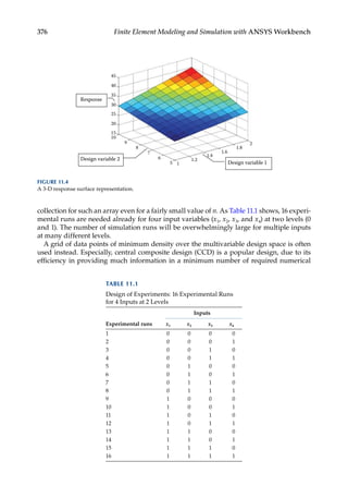
392. 377
Design Optimization
experiments [17]. CCD enables an efficient construction of a second-order fitting model.
As illustrated in Figure 11.5, a typical face-centered CCD for three design variables (x1, x2,
and x3) at 3 ­
levels suggests the use of 15 design points, compared to 33 possible combina-
tions of the full design. The 15 design points are marked as back dots in Figure 11.5. Each
design point corresponds to a design scenario. By using the CCD, the maximum amount of
information can be extracted while requiring a significantly reduced number of numerical
experiments.
11.4.2 Response Surface Optimization
After the design space is sampled through an experimental design such as CCD, a response
dataset (e.g., the maximum deformation and stress results) can be readily obtained for a
design scenario through the finite element simulation. The response datasets, with each
dataset corresponding to a simulation scenario, are then used to fit the response surface
models. These models are interpolation models that can provide continuous variation of
the responses with respect to the design variables (see Figure 11.4).
In the optimizer, a designer sets up a design objective and constraints. For optimization
with multiple objectives, the relative importance of different objectives and constraints can
be specified. Using the fitted response surface models, the feasible region, that is, the region
satisfying all design constraints can be identified in the design space. The best design can-
didate is then determined by searching for the best available value of the objective func-
tion over the entire design space’s feasible region.
In the next section, we will use ANSYS Workbench to optimize an L-shaped structure
using the above-mentioned techniques.
11.5 Case Studies with ANSYS Workbench
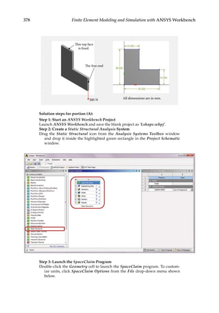
Problem Description: Determine if weight reduction pockets can be generated in the
L-shaped structure shown below. The structure is 2 mm thick and is made of structural
steel. The boundary and loading conditions are specified as follows: A downward force of
300 N is applied at the bottom edge of the free end, and the top face of the L-shape is fixed.
The allowed maximum deformation in the structure is 0.3 mm. A) Perform topology opti-
mization to achieve 75% weight reduction. B) Redesign the structure based on the results
from topology optimization, and conduct parametric optimization to minimize weight
subject to the deformation constraint.
x1
x2
x3
FIGURE 11.5
A face-centered central composite design for three design variables.

393. 378 Finite Element Modeling and Simulation with ANSYS Workbench
All dimensions are in mm.
This top face
is fixed.
300 N
The free end
Solution steps for portion (A):
Step 1: Start an ANSYS Workbench Project
Launch ANSYS Workbench and save the blank project as ‘Lshape.wbpj’.
Step 2: Create a Static Structural Analysis System
Drag the Static Structural icon from the Analysis Systems Toolbox window
and drop it inside the highlighted green rectangle in the Project Schematic
window.
Step 3: Launch the SpaceClaim Program
Double-click the Geometry cell to launch the SpaceClaim program. To custom-
ize units, click SpaceClaim Options from the File drop-down menu shown
below.

394. 379
Design Optimization
The following SpaceClaim Options window will show up. Click Units from the left
panel, and select Millimeters from the drop-down list of Length. Next, change the
Minor Grid Spacing to 5mm. Click OK to save your changes and close the window.

395. 380 Finite Element Modeling and Simulation with ANSYS Workbench
Step 4: Create the Geometry
Right-click anywhere in the Graphics Window, and click Select New Sketch
Plane from the drop-down context menu.
Mouse over x-y plane, and click to select the highlighted x-y plane. This will
change the sketch plane from the default x-z plane (shown above) to the x-y
plane (shown below).

396. 381
Design Optimization
Click Plan View on the toolbar to view the sketch grid head-on.
Click Sketch Mode on the Design tab to begin a sketch. Click on the Line icon.
Draw a sketch of the L-shape on the XY Plane, as shown below. To draw a line,
click a start point and then an end point in the sketch grid. The horizontal
distance is 35mm betweem Points 1 and 2, and 15mm between Points 5 and
6, respectively. The vertical distance is 35mm betweem Points 1 and 6, and
15mm between Points 2 and 3, respectively. When necessary, press the Esc key
to end the line creation.

397. 382 Finite Element Modeling and Simulation with ANSYS Workbench
Click on the Home icon for home view, and click on the Pull icon. Click on the
L-shape surface from the Graphics Window, and pull the surface along z-axis.
While pulling the surface, type 2mm in the text box for distance, and hit the
Enter key. A 2mm thick solid body will be created, as shown below.
Step 5: Launch the Static Structural Program
Double-click on the Model cell to launch the Static Structural program. Change
the Units to Metric (mm, kg, N, s, mV, mA).

398. 383
Design Optimization
Step 6: Generate Mesh
Click on Mesh in the Outline tree. In the Details of “Mesh”, enter’1.0’ for 1mm for
the Element Size. Right-click on Mesh and select Generate Mesh.
Step 7: Apply Boundary Conditions
Right-click on Static Structural (A5). Choose Insert and then Fixed Support
from the context menu. Click on the top face, and apply it to the Geometry
selection in the Details of “Fixed Support”. The top face of the L-shape is now
fixed as shown below.

399. 384 Finite Element Modeling and Simulation with ANSYS Workbench
Step 8: Apply Loads
Right-click on Static Structural (A5). Choose Insert and then Force. In the
Details of “Force”, change Define By to Components. Apply a -300 N force for
Y Component to the bottom edge of the rightmost face, as shown below.
Step 9: Retrieve Solution
Insert a Total Deformation item by right-clicking on Solution (A6) in the Outline
tree.
Insert an Equivalent Stress item by right-clicking on Solution (A6) in the Outline
tree.
Right-click on Solution (A6) in the Outline tree and select Solve. The program
will start to solve the model. After completion, click Total Deformation in the
Outline to review the total deformation results.

400. 385
Design Optimization
Select Equivalent Stress in the Outline to review the von-Mises stress distribu-
tion. As we can see from the stress results, there is a large area of blue which
means the equivalent stress in this area is almost zero. Therefore, we can opti-
mize the L-shaped structure in order to reduce the overall mass and just keep
the material that is required. Exit the Static Structural program.
Step 10: Launch the Topology Optimization
Drag the Topology Optimization icon from the Analysis Systems Toolbox and
drop it onto the Solution cell of the highlighted Static Structural system in
the Project Schematic.

401. 386 Finite Element Modeling and Simulation with ANSYS Workbench
This will share data from the Static Structural analysis and create a Topology
Optimization analysis. Double-click on the Setup cell to launch the Topology
Optimization interface.
Step 11: Setup the Topology Optimization
In the Multiple Systemsprogram that launches, note thatTopology Optimization
already excluded the regions of the Boundary Conditions from the optimiza-
tion problem, and it chose the full body of the L-shape as the Design Region
by default. Accept this default setup.

402. 387
Design Optimization
For the Objective, the default setup is to minimize the Compliance, which is
equivalent to maximize the structural stiffness. Accept this default setup.
For the Response Constraint, we can choose exactly what response we want to
add constraints, e.g., constraining on the mass, volume, von-Mises stress, dis-
placement or reaction forces. Here we want to achieve 75% weight reduction.
Therefore, we select Mass for Response, and set Percent to Retain as 25%.

403. 388 Finite Element Modeling and Simulation with ANSYS Workbench
Step 12: Retrieve Solution from Topology Optimization
In the Project tree, select Solution (B6). In the Details of “Solution (B6)”, make
sure that the Export Topology (STL file) in Post Processing is set to Yes. This
will enable us to export the optimized design as STL file afterwards.
Next, right-click on Solution (B6), and click Solve. When it starts running, click
on Topology Density Tracker in the Project tree to track the topology optimi-
zation process.

404. 389
Design Optimization
Once it is done, click on Topology Density in the Project tree to review results.
Click on the Play button in Animation to view the iterations. The region
marked in gray is suggested as the optimal shape for the design under the
given loads. Close the Multiple Systems program.
Solution steps for portion (B):
Step 1: Transfer the Optimized Result to a new Static Structural System
In the Project Schematic, right-click on Results and click Transfer to Design
Validation System. This will transfer the optimized results to a new Static
Structural System.

405. 390 Finite Element Modeling and Simulation with ANSYS Workbench
Note that now the Results of the Toplogy Optimization analysis is taken as the
input for the Geometry of the Static Structural analysis, as shown below.
Right-click on the Results cell of Topology Optimization, click Update. After
the update is done, a green Checkmark should appear for the Results cell of
Topology Optimization.

406. 391
Design Optimization
Next, right-click on the Geometry cell of the new Static Structural system, and
click Update.
Once update is complete, double-click on the Geometry cell of the new Static
Structural system to launch the SpaceClaim. Both the original L-shape and
the optimized shape are now imported into SpaceClaim. As shown below, the
edges of the optimized shape are rough. This geometry needs to be repaired,
as it is not so easy to manufacture.

407. 392 Finite Element Modeling and Simulation with ANSYS Workbench
Next, click SpaceClaim Options from the File drop-down menu shown below.
The following SpaceClaim Options window will show up. Click Units from the
left panel, and select Millimeters from the drop-down list of Length. Next,
change the Minor Grid Spacing to 5mm. Click OK to save your changes and
close the window.

408. 393
Design Optimization
Step 2: Create a New Sketch
Uncheck the 1st SYS-1 item in the Structure Tree to hide the original L-shape.
Click on the Sketch Mode icon, and click on the front face of the optimized
shape in the Graphics Window.
The following will be created as a result.

409. 394 Finite Element Modeling and Simulation with ANSYS Workbench
Click and drag to pull out a selection box in the Graphics Window. Draw a box
that encloses the entire bracket to select all the edges, as shown below. Next,
click on the Copy button to copy this to clipboard.
Click on the Paste button to paste all the selected edges onto the new sketch
plane.

410. 395
Design Optimization
Uncheck the 2nd SYS-1 item in Structure Tree to show only the edges.
Step 3: Simplify the Curves
To simplify curves, click the Fit Curves icon under the Repair tab. Accept the
default Find Options of a Maximum distance of 0.16mm, and check Lines and
Arcs under Fix Options. Click the Checkmark in the Graphics Window to fit
edges automatically into simpler curves.

411. 396 Finite Element Modeling and Simulation with ANSYS Workbench
The curves will turn into the following sketch. Note that there are still short lines
in between points 1 and 2, points 3 and 4, and points 5 and 6, which we need
to repair further.
Click on the Trim Away icon under the Design tab. In the Graphics Window,
click on the line segments in between points 1 and 2, 3 and 4, and 5 and 6, to
trim them away, as shown below.

412. 397
Design Optimization
Click on the Line icon under the Design tab. Create 3 straight lines, in between
points 1 and 2, points 3 and 4, and points 5 and 6, respectively, as shown below.
Click on the Trim Away icon under the Design tab. Click on the short lines around
corners to trim them away, as shown below. Make sure each edge has only one
line segment.

413. 398 Finite Element Modeling and Simulation with ANSYS Workbench
Click on the Create Rounded Corner icon under the Design tab. Click each pair
of adjacent lines to create a rounded corner with 2mm radius, as shown below.
Note that the line segments a, b, c and d may not be long enough to accommo-
date this fillet radius.
To fix that, the 4 line segments (a, b, c and d) may need to be extended. Click
the Create Corner icon under the Design tab to create two corners between
the 4 lines. To create a corner, click one side and then the adjacent side in the
Graphics Window.

414. 399
Design Optimization
Now click on the Create Rounded Corner icon under the Design tab. Click a
rounded corner of 2mm radius, as shown below, for the line segments a, b, c
and d.
Step 4: Create an Extruded Part
Click on the Pull icon under the Design tab. Click on the front face in the Graphics
Window. The face will be highlighted in orange as shown below. Click on the
Ruler in the mini-toolbar.

415. 400 Finite Element Modeling and Simulation with ANSYS Workbench
Click on the orange face to highlight the face again in the Graphics Window. Pull
the face along z-axis, and press the spacebar in keyboard to enter a value of
2mm in the highlighted field.
Click on the letter P next to the value of 2mm in the Graphics Window. A group
named “Group1” will be created, as shown in the Information messagebox
below.

416. 401
Design Optimization
Click on the Groups tab on the left panel to view groups. Click on the Ruler
dimension next to Group1 under Driving Dimensions to view its numeric
value of 2mm.
Right-click on the Group1 under Driving Dimensions, and select Rename from
the drop-down menu. Change the name of Group1 to Thickness, as shown
below.

417. 402 Finite Element Modeling and Simulation with ANSYS Workbench
Uncheck Surface in the Structure Tree to show only the solid part. Right-click
on Surface and the first SYS-1 in the Structure Tree, and click Suppress for
Physics in the drop menu. Items suppressed for physics are not imported for
subsequent physical analysis. Make sure that all other items except for Solid in
the Structure Tree are suppressed for physics. Exit SpaceClaim.
Step 5: Retrieve Solution from Simulation
In Project Schematic, double-click the Model cell of the new Static Structural
system. Click Yes on the popup menu to confirm reading upstream data. The
Static Structural Program is now launched.

418. 403
Design Optimization
In the Details of Mesh, change the Size Function under Sizing to Proximity and
Curvature. Right-click on the Mesh in the Project Outline and click Generate
Mesh. The following mesh will appear.
Click on the top face in the Graphics Window, and apply it to the Geometry selec-
tion in the Details of “Fixed Support”. The top face of the L-shape is now fixed
as shown below.

419. 404 Finite Element Modeling and Simulation with ANSYS Workbench
Click on the Edge filter. Then click on the bottom edge in the Graphics Window,
and apply it to the Geometry selection in the Details of “Force”. A 300N force
will be applied to the edge along negative Y, as shown below.
Right-click on Solution (C6) in the Outline tree and select Solve. The program
will start to solve the model. After completion, click Total Deformation in
the Outline to review the total deformation results. In the Details of “Total
Deformation”, click on the empty box left to Maximum under Results, and a
letter P will be marked in the box indicating it is a parameter.

420. 405
Design Optimization
Next, click on SYS-2Solid in the Outline Tree. In the Details of “SYS-2Solid”,
click on the empty box left to Mass under Properties, and a letter P will appear
indicating it is a parameter. Exit the Static Structural program.
Step 6: Explore the Parameter Set
Note that a Parameter Set menu has been added to the Project Schematic, as
shown below.
Double-click the Parameter Set in the Project Schematic. The input parameters
(design variables) and output parameters (responses) are listed with their

421. 406 Finite Element Modeling and Simulation with ANSYS Workbench
corresponding base values in the Outline of All Parameters window. In the
Table of Design Points, the current design is shown as the only design point.
Close the Parameter Set tab to return to Project Schematic.
Step 7: Create Response Surface Optimization
Double-clicktheResponseSurfaceOptimizationunderneathDesignExploration
from the Toolbox. A Response Surface Optimization system will be added to
the project schematic. The optimization system is linked to the Parameter Set
indicating that it has access to the design and response parameters. Double-
click on the Design of Experiments tab in the project schematic.

422. 407
Design Optimization
Step 8: Generate a DOE Table
In the Outline of Schematic, click on P1-Thickness. The default Lower Bound
and Upper Bound values for P1-Thickness are listed as shown below. We will
accept these default values in the design exploration.
Next, click on Design of Experiments in the Outline of Schematic. In the
Properties of Outline, turn on Preserve Design Points After DX Run. Change
the Design Type to Face-Centered.

423. 408 Finite Element Modeling and Simulation with ANSYS Workbench
In the toolbar, click Preview. A DOE table listing 5 design points is generated.
Then click Update in the toolbar to run finite element simulations for the 5
different design scenarios. It will take a while to finish running all the simula-
tions. After completion, review the 5 design points (simulation results) listed
in the Table of Outline. Close the entire Design of Experiments tab to return
to Project Schematic.
Step 9: Build Response Surface
Double-click on the Response Surface tab in the following Project Schematic.

424. 409
Design Optimization
Click on Response Surface in the upper left panel of Outline of Schematic. Turn
on the two options under Design Points in the lower left panel of Properties
of Outline. Next, click Update to create the response surface.
To view the response, click on Response in the upper left panel of Outline of
Schematic. The response chart of the maximum total deformation as a func-
tion of thickness is shown below. Review the response chart, and close the
Response Surface tab to return to Project Schematic.

425. 410 Finite Element Modeling and Simulation with ANSYS Workbench
Step 10: Set Up Objectives and Constraints
Double-click on the Optimization tab in the following Project Schematic.
Click on the Objectives and Constraints tab in the Outline of Schematic. Set
up the objective and constraints as shown below in the right panel of Table of
Schematic.

426. 411
Design Optimization
Click on Optimization in the Outline of Schematic. Select Screening for Method
Name in the Properties of Outline. Click Update in the toolbar.
Three candidates for best design are now listed in the Table of Schematic. Review
the best design (Candidate Point 1) in the Candidate Points table. Note that
three candidates are listed here because Maximum Number of Candidates is
set to 3 in the lower left Properties of Outline table. Close the Optimization
tab to return to Project Schematic.

427. 412 Finite Element Modeling and Simulation with ANSYS Workbench
Step 11: Update Current Design
Double-click on the Parameter Set in the Project Schematic.
In the right Table of Design Points shown below, DP1 achieves the best result
in minimizing the weight while meeting the deformation requirement. It has
a value of 1.8mm for Thickness. We will now update the current design with
this design point (DP1), which can then be served as the base case for another
round of optimization iteration if needed. Right-click on the DP1 in the Table
of Design Points, and select Copy inputs to Current in the drop-down menu.
This will update the Current design point with the selected design point DP1.

428. 413
Design Optimization
Next, right-click on the Current tab in the Table of Design Points, and select
Update Selected Design Points in the drop menu. This will update the results
of the Current design point. After done, close the Parameter Set tab to return
to Project Schematic.
Double-click the Geometry tab of the second Static Structural System in the
Project Schematic to open SpaceClaim.

429. 414 Finite Element Modeling and Simulation with ANSYS Workbench
The geometry is now updated in Graphics Window based on the current design
point (1.8mm for Thickness), as shown below. Close the SpaceClaim program.
Double-click on the Results tab of the second Static Structural System in
Project Schematic to view the updated deformation results from the Static
Structural – Mechanical program. Close Static Structural and save project.

430. 415
Design Optimization
11.6 Summary
In this chapter, we briefly discussed design optimization problems and the type of
optimizations. We also learnt how to apply FEA in design optimization studies. A case
study is demonstrated using ANSYS Workbench to reduce the weight of an L-shaped
structure.
11.7 Review of Learning Objectives
Now that you have finished this chapter you should be able to
1. Understand the basic concepts in design optimization and the steps in conducting
an optimization of a design with the FEA
2. Perform optimization of structure designs using ANSYS Workbench
PROBLEMS
11.1 The 3-D design space of a steel bridge structure is 6 m long, 2 m tall, and 1 m wide,
as shown below. Suppose the structure is fixed on the bottom two edges and is
applied a uniform pressure load on the top surface. Perform topology optmiza-
tion of the bridge using the given design space to achieve 80% weight reduction.
11.2 The following 1 m × 1 m square plate with a center hole of diameter 0.4 m is made
of structural steel and has a thickness of 0.1 m. Suppose the plate is fixed on the
left upper and lower edges, and is applied a downward force of 1000 N on the
upper right edge. Perform topology optmization of the plate to achieve a 60% and
90% weight reduction, respectively.

431. 416 Finite Element Modeling and Simulation with ANSYS Workbench
11.3 Optimize the stiffened aluminum panel design with clamped edges as shown
below. In the initial design, the 100 in. × 100 in. panel has a thickness of 0.5 in. The
stiffeners are each 100 in. long, 5 in. tall, and 0.25 in. thick, and divide the panel
evenly into eight blocks of the same area. The design variables, that is, the panel
thickness t, the longitudinal stiffener thickness tlong, and the lateral stiffener thick-
ness tlat, have the following range of variations: . . . ., . .
0 4 0 6 0 2
in in in
≤ ≤ ≤
t tlong
≤ ≤ ≤
0 3 0 2 0 3
. ., . . .
in and in in.
tlat The optimization aims to minimize the
panel’s weight subject to the constraint of the panel’s fundamental frequency
fbase ≥ 130 Hz.
Panel thickness t
Longitudinal stiffener
thickness tlong
Lateral stiffener
thickness tlat
11.4 Optimize the design of the following L-shaped bracket made of structural
steel with Young’s modulus E = 200 GPa and Poisson’s ratio ν = 0.3. In the ini-
tial design, the L-shape has a length L = 8 cm, a height h = 3 cm, and an extru-
sion depth d = 4 cm, and is rigidly connected to a rectangular block of size
3 cm × 8 cm × 1 cm, as shown below. The bracket is fixed on the right end. A
uniform pressure of 100 N/cm2 is applied on the protruding top face on the left.
The design variables, that is, L, h, and d, have the following range of variations:
6 cm ≤ L ≤ 8 cm, 2.5 cm ≤ h ≤ 3 cm, and 3 cm ≤ d ≤ 4 cm. The optimization aims to
minimize the bracket weight subject to the maximum allowed displacement limit
of 0.1 mm and stress limit of 100 MPa.
All dimensions are in
centimeters.
Length L
Height h
Depth d
1.000
8.000
3.000
1.000
R1.000

432. 417
Design Optimization
11.5 Perform topology and size optimization of the following bookshelf bracket
design. The bracket is 2 mm thick and is made of structural steel. The vertical
side of the bracket is fixed, and the horizontal side is applied a uniform pressure
of 25 MPa. (a) The objective of the topology optimization is to achieve a weight
reduction of 60%. (b) Redesign the bracket based on the results from topology
optimization. For the parametric optimization of the redesigned bracket, mini-
mize the bracket weight subject to the maximum allowed deformation constraint
of 0.5 mm and stress constraint of 100 MPa.
20 cm
20 cm
11.6 The original design space along with the constraints and loading conditions is
given below for structural optimization of a bike frame. The coordinate dimen-
sions are all in millimeters. Assume a 5 mm thickness for the design space and
perform topology optimization for the frame structure to achieve a weight reduc-
tion target of 60% and 80%, respectively. Use structural steel for the frame and
discuss on the results of optimization.
C (439, 405)
D (874, –276)
Initial design range coordinates The constraints and loads at the head,
seat, and pedal positions.
A (40, 83)
B (0, 0)
E (620, 83)
71 N
406 N
274 N
69.2 N
1960 N
200 N
11.7 The following heat sink consists of a 1 m tall central tube and 12 radial fins
that are uniformly distributed every 30°C around the central tube. The central
tube has an outer diameter of 0.4 m and an inner diameter of 0.36 m. Each fin is
0.048 m wide, 0.4 m long, and 1 m tall. The vapor temperature inside the tube
is 315°C with a heat transfer coefficient of 2.94 × 105 W/(m2°C). The surrounding

433. 418 Finite Element Modeling and Simulation with ANSYS Workbench
air temperature is 0°C with a heat transfer coefficient of 40.88 W/(m2°C). The
heat sink is made of aluminum alloy with a thermal conductivity of 175 W/
(m K), a density of 2770 kg/m3, and a specific heat of 870 J/(kg K). Optimize
the fin width W and the fin length L to minimize the use of material while
achieving a minimum heat dissipation of 75 kW per unit length. The design
variables W and L have the following range of variations: 0.03 m W 0.052 m,
and 0.2 m L 0.45 m.
L
W
11.8 The original design space along with the constraints and loading conditions is
given below for structural optimization of a chair. Assume that the chair is made
of Douglas fir with E = 104 MPa and ν = 0.3. The chair is subjected to two surface
loads with force magnitudes of 980 and 98 N, respectively, as shown in the figure.
The four corners at the bottom of the chair are fixed. Optimize the chair design to
achieve a 90% weight reduction.
1.4 m
0.6 m
0.6 m
0.6 m
Surface B
FA
= 980 N
FB
= 98 N
Surface A
0.8 m

434. 419
12
Failure Analysis
12.1 Introduction
Structures such as bridges, aircraft, and machine components can fail in many different
ways. An overloaded structure may experience permanent deformation, which can lead
to compromised function or failure of the entire structure. When subjected to millions of
small repeated loads, a structure may have a slow growth of surface cracks that can cause
material strength degradation and a sudden failure. When a slender structure is loaded
in compression, it may undergo an unexpected large deformation and lose its ability to
carry loads. Failure analysis plays an important role in improving the safety and reliabil-
ity of an engineering structure. In this chapter, we will discuss some of the topics related
to structural failure analysis. The concepts of static, fatigue, and buckling failures will be
introduced, along with examples using ANSYS® Workbench.
12.2 Static Failure
Under static loading conditions, material failure can occur when a structure is stressed
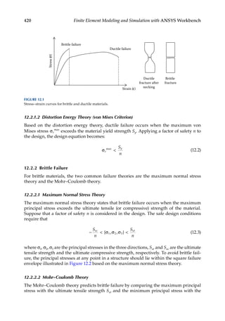
beyond the elastic limit. There are two types of material failures from static loading,
namely, ductile failure and brittle failure. The main difference between the two failure
types is the amount of plastic deformation a material experiences before fracture. As
illustrated in Figure 12.1, ductile materials tend to have extensive plastic deformation
before fracture, while brittle materials are likely to experience no apparent plastic defor-
mation before fracture. For more information on ductile and brittle failure, please see
Reference [18].
12.2.1 Ductile Failure
In this section, two common theories on ductile failure, that is, the maximum shear stress
theory (or Tresca Criterion) and the distortion energy theory (or von Mises Criterion), are
reviewed.
12.2.1.1 Maximum Shear Stress Theory (Tresca Criterion)
According to the maximum shear stress theory, ductile failure occurs when the maximum
shear stress τmax exceeds one half of the material yield strength Sy. Suppose that a factor of
safety n is considered in the design. The design equation is given as
τmax
S
n
y
2
(12.1)

435. 420 Finite Element Modeling and Simulation with ANSYS Workbench
12.2.1.2 Distortion Energy Theory (von Mises Criterion)
Based on the distortion energy theory, ductile failure occurs when the maximum von
Mises stress σe
max
exceeds the material yield strength Sy. Applying a factor of safety n to
the design, the design equation becomes:
σe
y
S
n
max
(12.2)
12.2.2 Brittle Failure
For brittle materials, the two common failure theories are the maximum normal stress
theory and the Mohr–Coulomb theory.
12.2.2.1 Maximum Normal Stress Theory
The maximum normal stress theory states that brittle failure occurs when the maximum
principal stress exceeds the ultimate tensile (or compressive) strength of the material.
Suppose that a factor of safety n is considered in the design. The safe design conditions
require that
−
S
n
S
n
uc ut
{ , , }
σ σ σ
1 2 3 (12.3)
where σ1, σ2, σ3 are the principal stresses in the three directions, Sut and Suc are the ultimate
tensile strength and the ultimate compressive strength, respectively. To avoid brittle fail-
ure, the principal stresses at any point in a structure should lie within the square failure
envelope illustrated in Figure 12.2 based on the maximum normal stress theory.
12.2.2.2 Mohr–Coulomb Theory
The Mohr–Coulomb theory predicts brittle failure by comparing the maximum principal
stress with the ultimate tensile strength Sut and the minimum principal stress with the
Brittle failure
Strain (ε)
Ductile failure
Ductile
fracture after
necking
Brittle
fracture
Stress
(σ)
FIGURE 12.1
Stress–strain curves for brittle and ductile materials.

436. 421
Failure Analysis
ultimate compressive strength Suc. Suppose that a factor of safety n is considered in the
design. The safe design conditions require that the principal stresses lie within the hexago-
nal failure envelope illustrated above in Figure 12.3.
12.3 Fatigue Failure
Under dynamic or cyclic loading conditions, fatigue can occur at stress levels that are
considerably lower than the yield or ultimate strengths of the material. Fatigue failures are
σ3
Suc Sut
Suc
n
n
n
n
Sut
σ1
FIGURE 12.2
The square failure envelope for the maximum normal stress theory.
σ3
σ1
Sut
Sut
Suc
Suc
n
n
n
n
FIGURE 12.3
The hexagonal failure envelope for the Mohr–Coulomb theory.

437. 422 Finite Element Modeling and Simulation with ANSYS Workbench
often sudden with no advanced warning and can lead to catastrophic results. In this sec-
tion, theories related to fatigue failure are reviewed. For more details, we refer the reader
to Reference [18].
Design of components subjected to cyclic load involves the concept of mean and alter-
nating stresses (see Figure 12.4 for an illustration of a typical fatigue stress cycle). The
mean stress, σm, is the average of the maximum and minimum stresses in one cycle, that
is, σ σ σ
m = +
( ) .
max min /2 The alternating stress, σa, is one-half of the stress range in one
cycle, that is, σ σ σ
a = −
( ) .
max min /2 For most materials, there exist a fatigue limit, and
parts having stress levels below this limit are considered to have infinite fatigue life. The
fatigue limit is also referred to as the endurance limit, Se.
In the following, three commonly used fatigue failure theories, namely, Soderberg,
Goodman, and Gerber failure criteria, are presented.
12.3.1 Soderberg Failure Criterion
This theory states that the structure is safe if
σ σ
a
e
m
y
S S n
+
1
(12.4)
where σa is the alternating stress, σm the mean stress, Se the endurance limit, Sy the yield
strength, and n the factor of safety. When the alternating stress σa is plotted versus the
mean stress σm, the Soderberg line can be drawn between the points of σa e
S n
= / and
σm y
S n
= / . If the stress is below the line, then the design is safe. This is a conservative
criteria based on the material yield strength Sy (see Figure 12.5).
12.3.2 Goodman Failure Criterion
This theory states that the structure is safe if
σ σ
a
e
m
ut
S S n
+
1
(12.5)
where Sut is the ultimate tensile strength and n is the factor of safety. When the alternating
stress σa is plotted versus the mean stress σm, the Goodman line can be drawn between
Cycles
σm
σmin
σmax
σa
Stress
FIGURE 12.4
A typical fatigue stress cycle.

438. 423
Failure Analysis
the points of σa e
S n
= / and σm ut
S n
= / . If the stress is below the line, then the design is
safe. This is a less conservative criteria based on the material ultimate strength Sut (see
Figure 12.5).
12.3.3 Gerber Failure Criterion
This theory states that the structure is safe if
σ σ
a
e
m
ut
S S n
+






2
1 (12.6)
where Sut is the ultimate tensile strength and n is the factor of safety. When the alternating
stress σa is plotted versus the mean stress σm, the Gerber parabola can be drawn between the
points of σa e
S n
= / and σm ut
S n
= / . If the stress is below the parabola, then the design is safe.
This is a less conservative criteria based on the material ultimate strength Sut (see Figure 12.5).
In general, most structures will fail eventually after a certain number of cycles of
repeated loading. In fatigue life analysis, S–N curves are widely used for the life estima-
tion, especially in high-cycle fatigue situations where the cyclic loading is elastic and the
number of cycles to failure is large. An S–N curve (see Figure 12.6) relates the alternating
stress, σa, to the number of cycles to failure, Nf, and is generated from fatigue tests on
samples of the given material.
Most S–N curves are developed based on zero mean stress. However, many loading
applications involve a nonzero mean stress. The Soderberg, Goodman, and Gerber theo-
ries mentioned above can be used to estimate the mean stress effects on fatigue life. Note
that there is little difference in the three theories when the mean stress σm is relatively
small compared to the alternating stress σa.
Take the Gerber theory as an example. To estimate a structure’s fatigue life for a given
combination of mean stress σm and alternating stress σa, one may first solve for the effective
alternating stress σe, based on the following modified Gerber equation:
σ
σ
σ
a
e
m
ut
S n
+





 =
2
1 (12.7)
Gerber parabola
Goodman line
Soderberg line
n
Se
σa
n
Sy
n
Sut
σm
FIGURE 12.5
Fatigue diagrams showing various criteria of failure.

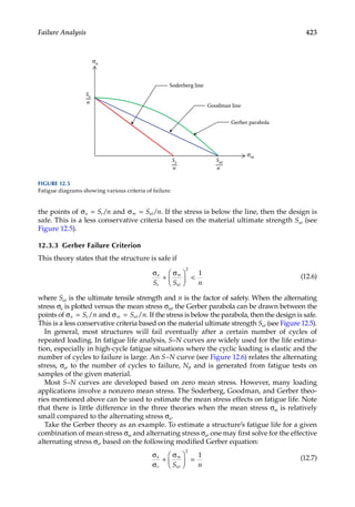
439. 424 Finite Element Modeling and Simulation with ANSYS Workbench
Once the effective alternating stress, σe, is obtained from Equation 12.7, the fatigue life
for the corresponding effective alternating stress σe can be determined from the S–N curve
of the given material (see Figure 12.6). If the effective alternating stress, σe, is kept below
threshold of the endurance limit, Se, the structure is considered to have an infinite life.
12.4 Buckling Failure
Under compressive loads, slender members such as columns can become structurally
unstable, leading to a sudden failure. The sudden loss of stability under compressive loads
is referred to as buckling [19]. Buckling failure usually occurs within the elastic range of
the material. The actual compressive stress in the structure at failure is often smaller than
the ultimate compressive strength of the material.
In buckling analysis, one may be interested in finding the critical load, that is, the
maximum compressive load a structure can support before buckling occurs, or the
buckling mode shapes, that is, shapes the structure takes while buckling. The criti-
cal load is a structure’s elastic stability limit, which is adequate to force the structure
to buckle into the first mode shape. A structure can potentially have infinitely many
buckling modes, and higher critical load values are required to trigger higher-order
buckling modes (see Figure 12.7 for an illustration of buckling failure of a slender col-
umn, and Figure 12.8 for different buckling mode shapes). Because buckling failure can
lead to catastrophic results, a high factor of safety (at least 3) is often used for critical
load calculations.
When developing a model for buckling, one should pay attention to the boundary con-
ditions as they have a considerable effect on a structure’s buckling behavior. For example,
a column with both ends pinned can buckle more freely than a column with both ends
fixed. Also note that bending moments acting on a structural member, for example, due
to ­
eccentricity of an axial load, may play a role in affecting buckling and should not be
neglected in the analysis in general.
Cycles to
failure (Nf)
Stress
(σ
a
)
Endurance limit
Fatigue life at
σe
σe
Se
FIGURE 12.6
Use of the S–N curve for fatigue life estimation.

440. 425
Failure Analysis
12.5 Case Studies with ANSYS Workbench
Problem Description: A dog-bone shaped specimen is examined for static, fatigue and
buckling failures. The specimen is made of structural steel with geometric dimensions
shown below. The bottom face of the specimen is fixed, and the top face of the specimen
is applied a static pressure load of 50 MPa. A) Determine whether or not the specimen
undergoes plastic deformation under the given static pressure load. B) If the static pres-
sure load is changed into a fully reversed cyclic load with a magnitude of 50 MPa, find
the life of the specimen, and also determine whether or not fatigue failure occurs in the
specimen assuming a design life of 106 cycles. C) Determine whether or not the specimen
buckles under the given static pressure load, and obtain the first three buckling mode
shapes.
(a) (b)
FIGURE 12.7
Buckling of a slender column: (a) load critical load, (b) load critical load. (http:/
/en.wikipedia.org/wiki/
Buckling.)
(a)
(b)
(c)
FIGURE 12.8
Buckling of a slender column: (a) unbuckled, (b) first buckling mode, and (c) second buckling mode.

441. 426 Finite Element Modeling and Simulation with ANSYS Workbench
The specimen
thickness is
0.75 mm.
15.000
R3.000
38.000
All dimensions are in mm.
5.000
8.000
Solution steps for portion (A and B):
Step 1: Start an ANSYS Workbench Project
Launch ANSYS Workbench and save the blank project as ‘Dogbone.wbpj’.
Step 2: Create a Static Structural Analysis System
Drag the Static Structural icon from the Analysis Systems Toolbox window
and drop it inside the highlighted green rectangle in the Project Schematic
window.
Step 3: Launch the SpaceClaim Program
Double-click the Geometry cell to launch SpaceClaim. To customize units,
select the SpaceClaim Options from the File menu to display the following
SpaceClaim Options window. Click Units from the navigation panel on the
left, and select Millimeters for Length. Next, change the Minor Grid Spacing
to 0.5mm. Click OK to save your changes and close the window.

442. 427
Failure Analysis
Step 4: Create the Geometry
Right-click anywhere in the Graphics Window. From the drop-down context
menu, choose Select New Sketch Plane.

443. 428 Finite Element Modeling and Simulation with ANSYS Workbench
Mouse over x-y plane, and click to select the highlighted x-y plane. This will
change the sketch plane to the x-y plane.
Click on the Plane View and the Sketch Mode icon on the Design tab. Click on
the Rectangle icon, and draw 3 rectangles on the XY Plane, as shown below.

444. 429
Failure Analysis
Click the Create Rounded Corner icon on the Design tab. In the Graphics
Window, draw 4 rounded corners, each with a radius of 3mm, as shown below.
Click the Trim Away icon, and trim away the unwanted lines in the sketch to
complete the dogbone profile.
Click on the Pull icon on the Design tab, and pull the sketch surface along
z-axis with a depth of 0.75mm to create a solid body, as shown below. Exit the
SpaceClaim.

445. 430 Finite Element Modeling and Simulation with ANSYS Workbench
Step 5: Launch the Static Structural Program
Double-click on the Model cell to launch the Static Structural program. Change
the Units to Metric (mm, kg, N, s, mV, mA).
Step 6: Generate Mesh
Click on Mesh in the Outline tree. In the Details of “Mesh”, enter’0.5 mm’ for the
Element Size. Right-click on Mesh and select Generate Mesh.
Step 7: Apply Boundary Conditions
Right-click on Static Structural (A5). Choose Insert and then Fixed Support
from the context menu. Click on the bottom face, and apply it to the Geometry
selection in the Details of “Fixed Support”. The bottom face of the dog bone
shape is now fixed as shown below.

446. 431
Failure Analysis
Step 8: Apply Loads
Right-click on Static Structural (A5). Choose Insert and then Pressure. In the
Details of “Pressure”, apply a 50MPa pressure to the top face, as shown below.
Step 9: Retrieve Static Analysis Results
First, insert a Total Deformation item by right-clicking on Solution (A6) in the
project Outline.
Then, insert an Equivalent Stress item by right-clicking on Solution (A6) in the
project Outline.
Next, right-click on Solution (A6) in the project Outline, and select Insert - Stress
Tool - Max Equivalent Stress. The initial yielding in the test sample may be
predicted by comparing the maximum von Mises stress in the specimen with

447. 432 Finite Element Modeling and Simulation with ANSYS Workbench
the tensile yield strength of the specimen material. The Stress Tool is used here
to show the safety factor results.
Right-click on Solution (A6) and select Solve. The computed total deformation,
von Mises stress and safety factor distributions are shown below. From the
static analysis results, it is apparent that the neck portion of the specimen will
not yield if loaded statically.
Step 10: Retrieve Fatigue Analysis Solution
Right-click on Solution (A6) in the Outline, and select Insert - Fatigue -
Fatigue Tool. In the Details of “Fatigue Tool”, set the Mean Stress Theory
to Goodman. Note that the default loading type is Fully Reversed constant
amplitude load, and that the default analysis type is the Stress Life type using
the von Mises stress calculations.

448. 433
Failure Analysis
Right-click on the Fatigue Tool in the Outline, and select Insert - Life. Next,
right-click on the Fatigue Tool and select Insert - Safety Factor. In the Details
of “Safety Factor”, change the Design life from the default value of 109 cycles
to 106 cycles. Lastly, right-click on the Fatigue Tool and select Evaluate All
Results. From the fatigue analysis results, the shortest life is at the undercut
fillets (19185 cycles) followed by the neck portion of the specimen. The neck
portion of the specimen has fairly small safety factor with a minimum value of
0.3979. The results show that the specimen will not survive the fatigue testing
assuming a design life of 106 cycles.
Solution steps for portion (C):
Step 1: Create a Linear Buckling Analysis System
In the Project Schematic window, right-click on the Solution cell of the Static
Structural analysis system and select Transfer Data to New - Eigenvalue
Buckling. An eigenvalue buckling analysis system will be added, with the
static structural results being used as initial conditions. The engineering data,
geometry and model will be shared by both analyses.

449. 434 Finite Element Modeling and Simulation with ANSYS Workbench
Step 2: Launch the Multiple Systems – Mechanical Program
Double-click the Setup cell of the Eigenvalue Buckling system to launch the
Multiple Systems – Mechanical program. Click on the Analysis Settings
under Eigenvalue Buckling (B5) in the Outline. In the Details of “Analysis
Settings”, set the Max Modes to Find to 3, and select No for Include Negative
Load Multiplier. The negative buckling load multiplier simply indicates that
reversing the applied loads (and scalling by the multiplier) will cause the
model to buckle.

450. 435
Failure Analysis
Step 3: Retrieve Linear Buckling Analysis Results
Insert three Total Deformation items by right-clicking on Solution (B6) in the
Outline. In the Details of “Total Deformation”, set Mode to 1. In the Details
of “Total Deformation 2”, set Mode to 2. In the Details of “Total Deformation
3”, set Mode to 3.
Right-click on Solution (B6) and select Solve to view the buckling modes. To
use the default window layout as shown below, select View - Windows -
Reset Layout from the top menu bar. Note that the load modifier for the first
buckling mode is found to be 0.78173. To find the load required to buckle the
structure, multiply the applied load by the load multiplier. For example, the
first buckling load will be 39.0865 MPa (0.78173 ×50MPa). The applied pressure
of 50MPa will cause the specimen to buckle, since it is larger than the critical
buckling load. In the Graph window, you can play the buckling animation.

451. 436 Finite Element Modeling and Simulation with ANSYS Workbench
The following figures show the first three buckling mode shapes. The correspond-
ing load multipliers for the 1st , 2nd and 3rd mode shapes are 0.78173, 2.0094
and 5.7321, respectively.
Note that the max value in the total deformation plots is scaled to 1 when display-
ing the buckling mode shapes. Here the deformation plot is used for buckling
mode shape visualization, with the actual values of deformation carrying no
physical meaning.
12.6 Summary
In this chapter, we briefly reviewed the static material failure theories (the ductile failure
and brittle failure theories), the fatigue failure theories for structures under low and cyclic
loading, and the buckling failure theory. An example of a dog-bone shaped specimen is
used to demonstrate how to conduct the static, fatigue, and buckling failure analyses using
the FEM with ANSYS Workbench.
12.7 Review of Learning Objectives
Now that you have finished this chapter you should be able to
1. Understand the failure theories for structures under static load
2. Understand the fatigue failure theories for structures under cyclic load

452. 437
Failure Analysis
3. Understand the buckling failure of a slender structure under static compressive
load
4. Perform static failure analysis of structures using ANSYS Workbench
5. Perform fatigue failure analysis of structures using ANSYS Workbench
6. Perform buckling failure analysis of structures using ANSYS Workbench
PROBLEMS
12.1 The following figure shows a simple bracket made of structural steel with Young’s
modulus E = 200 GPa and Poisson’s ratio ν = 0.3. The bracket has a front face pro-
file shown below and an extrusion depth of 12 cm. A through-hole of diameter
1.5 cm is centered on the bracket’s flat ends, one on each side. Suppose that the
bracket is fixed on the bottom, and is subjected to a fully reversed cyclic pressure
load of magnitude 10 MPa on the top face. Find the life of the bracket and deter-
mine whether or not fatigue failure occurs in the part assuming a design life of
106 cycles.
Cyclic loading
10.000
1.500
1.500
R3.000
8.000 1.500
1.500
12.000
8.000
1.500
All dimensions are in
centimeters.
12.2 The following figure shows a lifting bracket made of structural steel with Young’s
modulus E = 200 GPa and Poisson’s ratio ν = 0.3. The base portion of the bracket
is 20 cm long, 12 cm wide, and 3 cm deep. The fillet radius at the base corners is
1.75 cm. Four through-holes each of radius 1 cm are located symmetrically both
length wise and width wise in the base, with the hole centers being 12 cm apart by
6 cm apart. The upper portion of the base has a profile sketch shown below and is
3 cm thick. The bracket is fixed on the bottom. (1) Suppose the bracket is lifted by
a bearing load of 100 kN. Determine if the bracket can safely carry the given load.

453. 438 Finite Element Modeling and Simulation with ANSYS Workbench
(2) Find the life of the bracket if it is subjected to a fully reversed cyclic bearing
load of magnitude 50 kN.
R3.000
3.000
8.000
3.000
6.000
6.000
R1.500 All dimensions are in
centimeters.
12.3 The figure below shows a bracket made of structural steel with Young’s modu-
lus E = 200 GPa and Poisson’s ratio ν = 0.3. The rectangular base of the bracket is
12 cm long, 6 cm wide, and 3 cm deep. The midsection has an overall extrusion
depth of 1.6 cm and a profile sketch shown below. The hollow cylinder has an
inner radius of 1 cm, an outer radius of 2 cm, and a height of 4 cm. The central axis
of the cylinder is 12.5 cm away from the leftmost end of the bracket. The bracket
is fixed on the left end. (1) Determine if the bracket can safely carry the load when
a pressure of 800 N/cm2 is exerted on the inclined face of the midsection. (2) Find
the life of the bracket if it is subjected to a fully reversed cyclic pressure of magni-
tude 5 MPa on one side of the midsection as shown below.
All dimensions are in
centimeters.
Cyclic loading
4.000
8.000
6.000
12.4 The following figure shows an L-shaped bracket made of structural steel with
Young’s modulus E = 200 GPa and Poisson’s ratio ν = 0.3. The 4 cm thick L-shape
with the cross-sectional profile shown in the figure is rigidly connected to a rect-
angular base of size 3 cm × 8 cm × 1 cm. The bracket is fixed on the right end at
the base. A surface pressure of 10 MPa is exerted on the left end as shown below.
(1) Determine if static failure or buckling failure occurs in the bracket. (2) Find the

454. 439
Failure Analysis
life of the bracket if it is subjected to a fully reversed cyclic pressure of magnitude
10 MPa on the left end.
Pressure loading
1.000
R1.000
3.000
8.000
1.000
All dimensions are in
centimeters.
12.5 The following figure shows the cross-sectional profile of a 39 ft long straight rail-
road track. Use structural steel for the track with Young’s modulus E = 200 GPa
and Poisson’s ratio ν = 0.3. Assume the track is fixed on one end and subjected to a
pressure load along the axis of the track on the other end, that is, the cross section
at a distance of 39 ft from the fixed end. Determine the critical buckling load for
the railroad track.
1.375
All length dimensions are
in inches.
R0.500
1.125
105.00°
R0.500
0.375
R0.500
105.00°
2.250
0.375
6.000
12.6 The following two-bar assembly consists of four components made of struc-
tural steel with Young’s modulus E = 200 GPa, Poisson’s ratio ν = 0.3, and density
ρ = 7850 kg/m3. As shown in the figure below, the two bars are identical in size.
Each bar has a diameter of 2 cm and a length of 16 cm. The two identical end
blocks each has a thickness of 2 cm and a fillet radius of 1 cm at the round corners.

455. 440 Finite Element Modeling and Simulation with ANSYS Workbench
The distance of the gap in between the two blocks is 8 cm. The two bars are fixed
on the right ends, and subjected to a pressure load of 100 MPa on the left ends
as shown below. (1) Determine if static failure or buckling failure occurs in the
assembly. (2) Assuming a design life of 106, determine if fatigue failure occurs
in the assembly when subjected to a fully reversed cyclic pressure of magnitude
100 MPa on the left ends of the two bars.
2.000
R1.000
Loading
10.000
6.000
5.000
Fixed ends
All dimensions are in centimeters.
Use bonded for all contact regions.
12.7 The following figure shows a crank shaft made of structural steel with Young’s
modulus E = 200 GPa and Poisson’s ratio ν = 0.3. The crank shaft consists of three
identical horizontal rods and two identical vertical pieces. The rod is each 4 in. long.
The plate each has a thickness of 0.5 in. Along the four edges where the rods are con-
nected with the plates, a fillet of radius 0.2 in. is added to create round corners. The
crank shaft is fixed on the two ends and subjected to a fully reversed cyclic pressure
of magnitude 300 psi on the top face of the central rod as shown below. Assuming a
design life of 106, determine if fatigue failure occurs in the crank shaft assembly.
Cyclic loading
Fixed end
Fixed end
All dimensions are in inches.
R1.250
D1.800
2.750
R0.800
D1.800
4.250
2.750
1.250

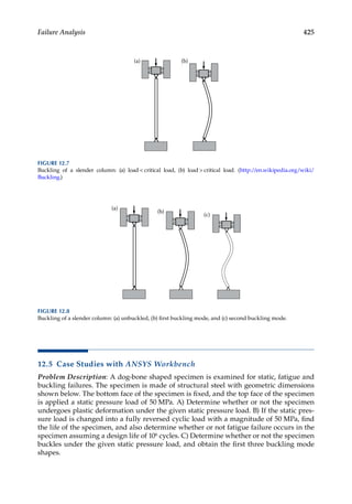
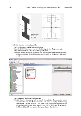
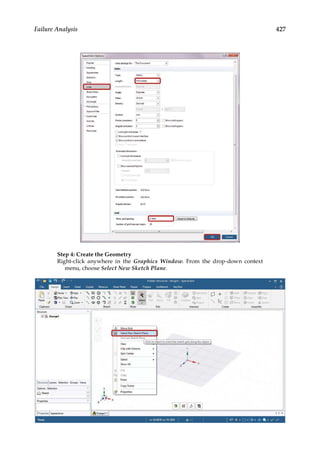
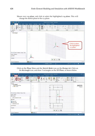
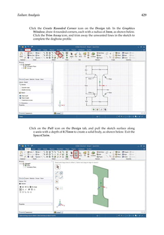
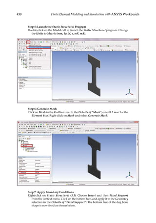
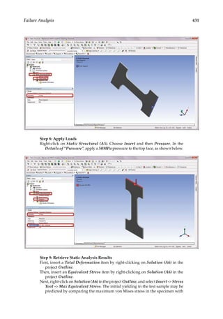
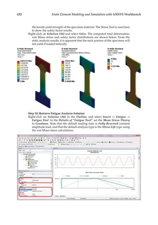
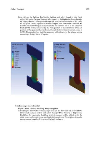
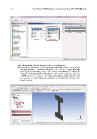
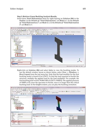
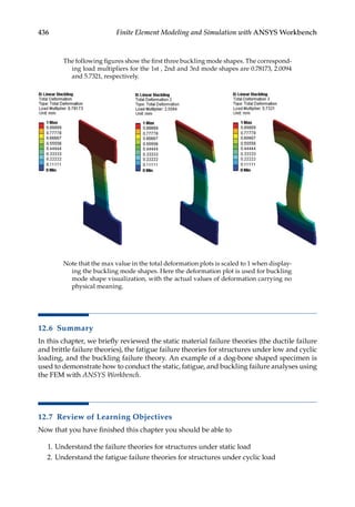
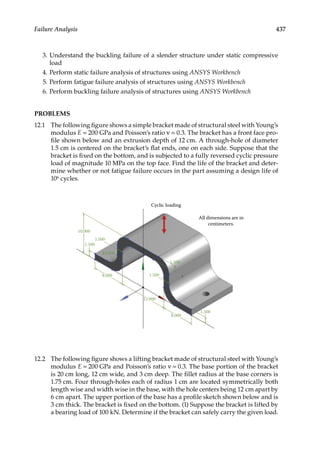
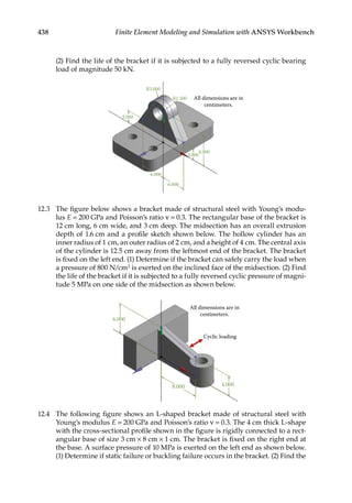
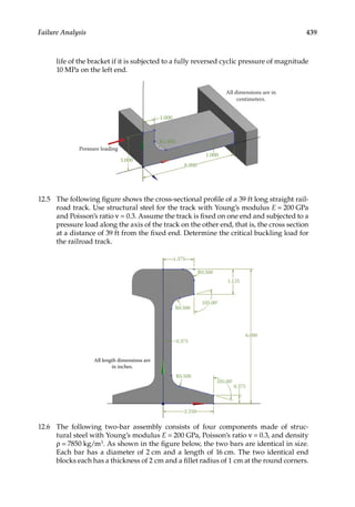
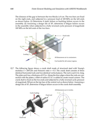
456. 441
Appendix 1: Review of Matrix Algebra
A.1 Linear System of Algebraic Equations
a x a x a x b
a x a x a x b
a x a
n n
n n
n
11 1 12 2 1 1
21 1 22 2 2 2
1 1
+ + + =
+ + + =
+
…
…
.......
n
n nn n n
x a x b
2 2 + + =
…
(A.1)
where x1, x2, …, xn are the unknowns.
In matrix form:
Ax b
= (A.2)
where
A x
= =












=
[ ] , {
a
a a a
a a a
a a a
ij
n
n
n n nn
11 12 1
21 22 2
1 2
…
…
… … … …
…
x
x
x
x
x
b
b
b
b
i
n
i
n
}
:
, { }
:
=














= =














1
2
1
2
b (A.3)
A is called an n × n (square) matrix, and x and b are (column) vectors with dimension n.
A.2 Row and Column Vectors
v w
= =










[ ]
v v v
w
w
w
1 2 3
1
2
3
(A.4)

457. 442 Appendix 1
A.3 Matrix Addition and Subtraction
For two matrices A and B, both of the same size (m × n), the addition and subtraction are
defined by
C A B
D A B
= + = +
= − = −
with
with
c a b
d a b
ij ij ij
ij ij ij
(A.5)
A.4 Scalar Multiplication
λ λ
A = [ ]
aij (A.6)
A.5 Matrix Multiplication
For two matrices A (of size l × m) and B (of size m × n), the product of AB is defined by
C AB
= =
=
∑
with c a b
ij ik
k
m
kj
1
(A.7)
where i = 1, 2,…, l; j = 1, 2,…, n.
Note that, in general, AB ≠ BA, but (AB)C = A(BC) (associative).
A.6 Transpose of a Matrix
If A = [aij], then the transpose of A is
AT
ji
a
= [ ] (A.8)
Notice that
( )
AB B A
T T T
= (A.9)

458. 443
Appendix 1
A.7 Symmetric Matrix
A square (n × n) matrix A is called symmetric, if
A A
= =
T
ij ji
a a
or (A.10)
A.8 Unit (Identity) Matrix
I =












1 0 0
0 1 0
0 0 1
…
…
… … … …
…
(A.11)
Note that AI = A, Ix = x.
A.9 Determinant of a Matrix
The determinant of square matrix A is a scalar number denoted by det A or |A|. For 2 × 2
and 3 × 3 matrices, their determinants are given by
det
a b
c d
ad bc





 = − (A.12)
and
det
a a a
a a a
a a a
a a a a a a
11 12 13
21 22 23
31 32 33
11 22 33 12 23










= + 3
31 21 32 13
13 22 31 12 21 33 23 32 11
+
− − −
a a a
a a a a a a a a a
(A.13)
A.10 Singular Matrix
A square matrix A is singular if det A = 0, which indicates problems in the system (non­
unique solutions, degeneracy, etc.).

459. 444 Appendix 1
A.11 Matrix Inversion
For a square and nonsingular matrix A (det A ≠ 0), its inverse A−1 is constructed in such a
way that
AA A A I
− −
= =
1 1 (A.14)
The cofactor matrix C of matrix A is defined by
C M
ij
i j
ij
= − +
( )
1 (A.15)
where Mij is the determinant of the smaller matrix obtained by eliminating the ith row and
jth column of A.
Thus, the inverse of A can be determined by
A
A
C
−
=
1 1
det
T
(A.16)
We can show that (AB)−1 = B−1A−1.
EXAMPLE A.1
(A)
a b
c d ad bc
d b
c a





 =
−
−
−






−1
1
( )
Checking:
a b
c d
a b
c d ad bc
d b
c a
a b
c d











 =
−
−
−











 =
−1
1 1 0
0 1
( )







(B)
1 1 0
1 2 1
0 1 2
1
4 2 1
3 2 1
2 2 1
1 1 1
3 2 1
1
−
− −
−










=
− −










=
−
( )
T
2
2 2 1
1 1 1










Checking:
1 1 0
1 2 1
0 1 2
3 2 1
2 2 1
1 1 1
1 0 0
0 1 0
0 0 1
−
− −
−




















=











If det A = 0 (i.e., A is singular), A−1 does not exist.
The solution of the linear system of equations (Equation 1.1) can be expressed as
(assuming the coefficient matrix A is nonsingular)
x A b
= −1
Thus, the main task in solving a linear system is to find the inverse of the coefficient
matrix.

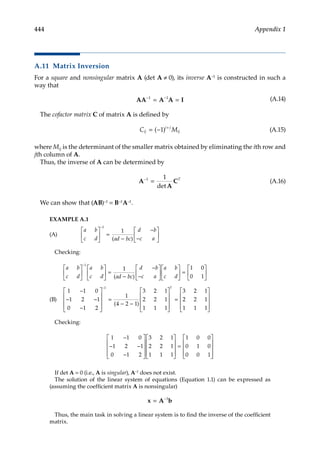
460. 445
Appendix 1
A.12 Solution Techniques for Linear Systems of Equations
• Gauss elimination methods
• Iterative methods
The two methods are briefly reviewed in Chapter 5.
A.13 Positive-Definite Matrix
A square (n × n) matrix A is said to be positive definite, if for all nonzero vector x of dimen-
sion n,
x Ax
T
0
Note that positive-definite matrices are nonsingular. We can show that all stiffness
matrices are positive definite and the above condition is a statement that the strain energy
in a structure should be positive if the structure is constrained and the stiffness matrix is
nonsingular.
A.14 Differentiation and Integration of a Matrix
Let A(t) = [aij(t)], then the differentiation is defined by
d
dt
t
da t
dt
ij
A( )
( )
=





 (A.17)
and the integration by
A( ) ( )
t dt a t dt
ij
= 





∫
∫ (A.18)

462. 447
Appendix 2: Photo Credits
Chapter 1
Figure 1.1(a) A train engine built with LEGO®.
(http:/
/lego.wikia.com/wiki/10020_Santa_Fe_Super_Chief)
Figure 1.3(a) Wind load simulation of an offshore platform.
(Courtesy ANSYS, Inc. http:/
/www.ansys.com/Industries/Energy/Oil++Gas);
Figure 1.3(b) Modal response of a steel frame building with concrete slab floors.
(http:/
/www.isvr.co.uk/modelling/)
Figure 1.3(c) Underhood flow and thermal management.
(Courtesy ANSYS, Inc. http:/
/www.ansys.com/Industries/Automotive/Application+
Highlights/Underhood)
Figure 1.3(d) Electric field pattern of antenna mounted on helicopter.
(Courtesy ANSYS, Inc. http:/
/www.ansys.com/Industries/Electronics++Semiconduc
tor/Defense++Aerospace+Electronics)
Chapter 2
Figure 2.1(a) Montreal Biosphere Museum.
(http:/
/en.wikipedia.org/wiki/Montreal_Biosph%C3%A8re)
Figure 2.1(b) Betsy Ross Bridge.
(http:/
/en.wikipedia.org/wiki/Betsy_Ross_Bridge)
Chapter 3
Figure 3.1(a) A car frame.
(http:/
/www.carbasics-1950.com/)
Figure 3.1(b) An exercise machine.
(http:/
/www.nibbledaily.com/body-by-jake-cardio-cruiser/)

463. 448 Appendix 2
Chapter 5
Figure 5.1(a) Reflective symmetry.
(http:/
/www.thinkingfountain.org/s/symmetry/butterflypattern.gif)
Figure 5.1(c) Rotational symmetry.
(http:/
/csdt.rpi.edu/na/pnwb/symmetry2a.html)
Figure 5.1(d) Translational symmetry.
(http:/
/library.thinkquest.org/16661/background/symmetry.1.html)
Chapter 6
Figure 6.1 An airplane made of numerous plate and shell structures.
(http:/
/en.wikipedia.org/wiki/Boeing_787_Dreamliner)
Chapter 8
Figure 8.7 Two equations for determining the proportional damping coefficients.
(From R. D. Cook, Finite Element Modeling for Stress Analysis (John Wiley Sons, Inc.,
Hoboken, NJ, 1995).)
Figure 8.13 Car crash analysis using the FEA (from LS-Dyna website).
(http:/
/www.dynaexamples.com/)
Chapter 10
Figure 10.1(a) Airflow around a tractor.
(Courtesy ANSYS, Inc. http:/
/www.ansys.com/Industries/Automotive/Application+
Highlights/Body)
Figure 10.1(b) Streamlines inside a combustion chamber.
(Courtesy ANSYS, Inc. http:/
/www.edr.no/en/courses/ansys_cfd_advanced_­
modeling_reacting_flows_and_combustion_in_ansys_fluent)
Chapter 12
Figure 12.7 Buckling of a slender column.
(http:/
/en.wikipedia.org/wiki/Buckling)

464. 449
References
1. O. C. Zienkiewicz, The birth of the finite element method and of computational mechanics,
International Journal for Numerical Methods in Engineering, 60, 3–10, 2004.
2. ANSYS Workbench User’s Guide, Release 14.5, ANSYS, Inc., 2012.
3. C. Felippa, Introduction to Finite Element Methods, Lecture Notes, University of Colorado at
Boulder (http://www.colorado.edu/engineering/cas/courses.d/IFEM.d/).
4. J. N. Reddy, An Introduction to the Finite Element Method, 3rd ed. (McGraw-Hill, New York, 2006).
5. O. C. Zienkiewicz and R. L. Taylor, The Finite Element Method, 5th ed. (McGraw-Hill, New York,
2000).
6. S. P. Timoshenko and S. Woinowsky-Krieger, Theory of Plates and Shells, 2nd ed. (McGraw-Hill,
New York, 1987).
7. R. D. Cook, Finite Element Modeling for Stress Analysis (John Wiley Sons, Inc., Hoboken, NJ,
1995).
8. K. J. Bathe, Finite Element Procedures (Prentice-Hall, Englewood Cliffs, NJ, 1996).
9. T. R. Chandrupatla and A. D. Belegundu, Introduction to Finite Elements in Engineering, 3rd ed.
(Prentice-Hall, Upper Saddle River, NJ, 2002).
10. Y. C. Fung, A First Course in Continuum Mechanics, 3rd ed. (Prentice-Hall, Englewood Cliffs, NJ,
1994).
11. P. Timoshenko and J. N. Goodier, Theory of Elasticity, 3rd ed. (McGraw-Hill, New York, 1987).
12. ANSYS Help System, Mechanical Applications—Mechanical User Guide, Release 14.5, ANSYS,
Inc., 2012.
13. R. D. Cook, D. S. Malkus, M. E. Plesha, and R. J. Witt, Concepts and Applications of Finite Element
Analysis, 4th ed. (John Wiley Sons, Inc., Hoboken, NJ, 2002).
14. S. Moaveni, Finite Element Analysis—Theory and Application with ANSYS, 3rd ed. (Prentice-Hall,
Upper Saddle River, NJ, 2007).
15. B. R. Munson, D. F. Young, and T. H. Okiishi, Fundamentals of Fluid Mechanics, 5th ed. (John
Wiley Sons, Inc., Hoboken, NJ, 2006).
16. ANSYS Help System, CFX—Modeling Guide, Release 14.5, ANSYS, Inc., 2012.
17. ANSYS Help System, Design Exploration User Guide, Release 14.5, ANSYS, Inc., 2012.
18. J. E. Shigley, C. R. Mischke, and R. G. Budynas, Mechanical Engineering Design, 7th ed. (McGraw-
Hill, New York, 2003).
19. F. P. Beer, E. R. Johnston, J. T. DeWolf, and D. F. Mazurek, Mechanics of Materials, 6th ed.
(McGraw-Hill, New York, 2011).

466. 451
Index
A
ANSYS Workbench, 3, 13; see also Case studies;
Finite element analysis (FEA)
menu bar, 16–17
project schematic, 14–16
toolbox, 14
user interface, 13, 14
working with cells, 16, 17
B
Bar element, 21, 23, 59; see also 1D elasticity
theory; Trusses
axially loaded elastic bar, 22
case study, 40–58
consistent mass matrix, 265
constitutive equations for, 68
distributed load, 27–28
element equilibrium equation, 25
element stress, 31–32
examples, 32
exercises, 59–63
lumped mass for 1D, 265
multipoint constraint, 37–40
notation for, 24
shape functions for, 25
stiffness matrix, 23–27
3D case, 31
2D case, 28–31
Bars and trusses, 40–58
BCs, see Boundary conditions (BCs)
Beam element, 70, 112; see also Beams
case study, 85–111
configurations for, 72
consistent mass, 266
distributed load, 74, 75
element stiffness equation, 71–74
examples, 76–85
exercises, 112–115
notion for, 71
stiffness matrix, 75, 82
Beams, 65, 112; see also Beam element
bending, 67
bending stiffness, 67–68
bending strain, 67
bending stress, 67
constitutive equations for, 68
deflection of, 66
Euler–Bernoulli beam, 65
exercise machine, 66
exercises, 112–115
governing equations for, 68
line model, 70
profiles, 69
shapes, 68
strong and weak axes, 69
support conditions, 69–70
theory, 65
Timoshenko beam, 65
Bending stiffness, 67–68, 69
Bending strain, 67
Bending stress, 67
flexure formula, 67
in plates, 189
Betsy Ross Bridge, 22, 447; see also Trusses
Boundary conditions (BCs), 33
exercises, 155
fluid flow modeling, 339
for heat conduction problems, 303
for plate bending, 191
structural loads, 224
support types, 223–224
for thick plates, 193
2D elasticity, 121, 222
Brittle failure, 420; see also Failure analysis
hexagonal failure envelope, 421
Mohr–Coulomb theory, 420–421
square failure envelope, 421
stress–strain curves, 419
stress theory, 420
Buckling failure, 424, 425; see also Failure
analysis
C
CAD, see Computer-aided design (CAD)
CAE, see Computer-aided engineering (CAE)
CAM, see Computer-aided manufacturing
(CAM)
Case studies; see also ANSYS Workbench
bars and trusses, 40–58
beams and frames, 85
design optimization, 377–414
failure analysis, 425–436
fluid analysis, 341

467. 452 Index
Case studies (Continued)
modeling and solution techniques, 168–182
plate and shell analyses, 199–213
structural vibration and dynamics, 277
thermal analysis, 308
thermal stress analysis, 325–329
3D elasticity, 230
2D elasticity, 137
CCD, see Central composite design (CCD)
Central composite design (CCD), 376–377
Central difference method, 273–274; see also
Transient response analysis
CFD, see Computational fluid dynamics (CFD)
Computational fluid dynamics (CFD), 337; see
also Fluid analysis
examples of, 338
N–S equations for particle motion, 338–339
practical aspects of, 339–341
Computer-aided design (CAD), 1
development process, 2
plate with hole, 4
Computer-aided engineering (CAE), 1
development process, 2
FEM, 1
Computer-aided manufacturing (CAM), 1
development process, 2
Computer-aided product development process, 2
Consistent mass matrix, 265–266
Constant strain triangle (CST or T3), 124; see also
Two-dimensional elasticity
area of triangle, 126
displacements, 125
element stiffness matrix, 126
Jacobian matrix, 128
natural coordinate system, 127
nodes, 124
shape functions, 126, 127
CST, see Constant strain triangle (CST or T3)
D
Damping, 266–267
coefficient determination, 267
damped natural frequency, 263
Damping ratio, 263, 266, 271
Degree of Freedom (DOF), 25
discrete Kirchhoff triangular element
with, 197
four-node quadrilateral element with, 196
multi-DOF system, 264
single DOF system, 262–264
six-node triangular element with 5
DOFs, 197
system with damping, 262
Design of experiments (DOE), 375
Design optimization, 373, 415
Black Box optimization schematic, 375
case studies, 377–414
CCD, 376–377
design of experiments, 375
design space exploration, 374–375
design variables, 374
exercises, 415–418
face-centered central composite design, 377
feasible region, 377
parametric optimization, 374
response surface optimization, 377
state variables, 374
stiffened panel with clamped edges, 375
3D response surface representation, 376
topology optimization, 373, 374
Design variables, 374
in DOE, 375
face-centered central composite
design, 377
Discrete Kirchhoff triangular (DKT), 197
Displacement-based FEM, 34, 167
Distortion energy theory, 420; see also Ductile
failure
DKT, see Discrete Kirchhoff triangular (DKT)
DOE, see Design of experiments (DOE)
DOF, see Degree of Freedom (DOF)
Ductile failure, 419; see also Failure analysis
design equation, 419
distortion energy theory, 420
maximum shear stress theory, 419
stress–strain curves, 419
Dynamic response analysis, see Transient
response analysis
Dynamics, 261
E
Eigenvalue problem (EVP), 268
Elasticity theory, 219; see also 1D elasticity
theory; Three-dimensional elasticity;
2D elasticity theory
boundary conditions, 222
displacement, 221
equilibrium equations, 221–222
state of stress, 220
strain components, 220
strain–displacement relation, 221
stress analysis, 222
stress components, 219
stress–strain relation, 220–221

468. 453
Index
3D elastic domain boundary, 222
Element equilibrium equation, 25
Engineering beam theory, see Euler–Bernoulli
beam
Error stress field, 168
Euler–Bernoulli beam, 65; see also Beams
deflection of, 66
simple beam bending, 67
EVP, see Eigenvalue problem (EVP)
F
Failure analysis, 419, 436; see also Brittle
failure; Ductile failure; Fatigue
failure
buckling failure, 424, 425
case studies, 425–436
exercises, 437–440
static failure, 419
Fatigue failure, 421; see also Failure analysis
exercises, 437–440
fatigue diagrams, 423
fatigue stress cycle, 422
Gerber failure criterion, 423–424
Goodman failure criterion, 422–423
S–N curve for fatigue life estimation, 424
Soderberg failure criterion, 422
FBD, see Free-body diagram (FBD)
FEA, see Finite element analysis (FEA)
FEM, see Finite element method (FEM)
Finite element analysis (FEA), 1, 17; see also
ANSYS Workbench; Finite element
method (FEM); Spring system
adaptive, 167–168
with ANSYS Workbench, 3
applications in engineering, 1
boundary and load conditions, 9
bumper and brackets, 275
car crash analysis using, 277
computer-aided product development
process, 2
displacement solutions, 167
for drag link, 223
elements in FEA model, 166
equation solving, 164–166
examples, 10–13
exercises, 18–19
history of, 3–4
model of truck, 163
models of mechanical systems, 163
procedure for, 4
solution convergence, 167
solution verification, 10
for thermal stress analysis, 305
Finite element method (FEM), 1, see Finite
element analysis (FEA)
discretization, 4
displacement-based, 34
solution of displacement, 166
symmetry properties and, 161
thermal problems modeling, 306
Flow simulations, 337
Fluid analysis, 337, 368; see also Fluid flow
modeling
case studies, 341
exercises, 368–372
fluid flow types, 337
fluid motion, 337
Navier–Stokes equations, 338
shear stress, 337
Fluid domain, 339
Fluid flow modeling, 339, 368; see also Fluid
analysis
airflow over a city block, 340
boundary conditions, 339–340
case studies, 341
exercises, 368–372
flow region, 339
fluid domain, 339
meshing, 339
pressure boundary, 340
resolution of mesh, 340
solution visualization, 340–341
Fourier heat conduction equation, 301
Frame, 65, 112; see also Beams
car, 66
exercise machine, 66
line model, 70
Free-body diagram (FBD), 262
Frequency response analysis, 271; see also
Structural vibration and dynamic
analyses
direct method, 272
examples, 276
modal method, 271–272
G
Gauss elimination, 164–165
Gauss–Seidel method, 165
Gerber failure criterion, 423; see also Fatigue
failure
Goodman failure criterion, 422–423; see also
Fatigue failure
Graphical-user interface (GUI), 13
GUI, see Graphical-user interface (GUI)

469. 454 Index
H
Harmonic response analysis, see Frequency
response analysis
Heat conduction
boundary conditions for, 303
equation, 301
exercise, 330
finite element formulation for, 303
heat-sink model, 306
Heat flow equation, 302
I
Identity matrix, see Unit matrix
Isoparametric element, 227
Isoparametric mapping, 227
Iterative methods, 164, 165–166
K
Kirchhoff plate theory, 189; see also Plate
theory
boundary conditions, 191
deflection and rotation of plate, 189
discrete Kirchhoff elements, 197
displacement, 190
equilibrium of plate, 190–191
example, 191–192
Kirchhoff plate elements, 195–196
strains, 190
stresses, 190
L
Line model, 70
Linear quadrilateral element, 130; see also Two-
dimensional elasticity
displacement field, 131
shape functions, 130
traction on, 133
Linear strain triangle (LST), 129; see also
Quadratic triangular element; Two-
dimensional elasticity
displacements, 130
shape functions, 129, 130
Linear system of algebraic equations, 441
Linear triangular element, see Constant strain
triangle (CST or T3)
LST, see Linear strain triangle (LST)
Lumped mass, 265
matrices, 264
1 for D bar element, 265
M
Mass matrices, 264
consistent, 265, 266
element, 265
lumped, 264
Matrix
addition and subtraction, 442
determinant, 443
differentiation, 445
integration, 445
inversion, 444
multiplication, 442
Matrix algebra, 441
addition and subtraction, 442
differentiation and integration, 445
linear system of algebraic equations, 441
matrix determinant, 443
matrix inversion, 444
multiplication, 442
positive-definite matrix, 445
row and column vectors, 441
scalar multiplication, 442
singular matrix, 443
solution techniques, 445
symmetric matrix, 443
transpose of matrix, 442
unit matrix, 443
Maximum normal stress theory, 420; see also
Brittle failure
Maximum shear stress theory, 419; see also
Ductile failure
Mindlin plate theory, 192; see also Plate theory
displacement and rotation, 192
governing equations and boundary
conditions, 193
Mindlin plate elements, 196
Modal method, 271, 274–275; see also Transient
response analysis
Modeling, 68
Modeling and solution techniques, 161, 182
adaptivity, 167–168
case study, 168–182
convergence of FEA solutions, 167
elements in FEA model, 166
equation solving, 164
error stress field, 168
example, 162, 164–166
exercises, 183–185
finite element solutions, 166–167
Gauss elimination, 164–165
iterative methods, 164, 165–166
relative energy error, 168

470. 455
Index
substructures, 163–164
symmetry, 161–162
Mohr–Coulomb theory, 420–421; see also Brittle
failure
Montreal Biosphere Museum, 22; see also
Trusses
MPC, see Multipoint constraint (MPC)
Multipoint constraint (MPC), 39–40
N
Navier–Stokes equations (N–S equations), 338
in CFD modeling, 338–339
3-in D Cartesian coordinates, 338
Newmark method, 274; see also Transient
response analysis
Newton’s law of motion, 262
Normal modes, 268
N–S equations, see Navier–Stokes equations
(N–S equations)
O
1D elasticity theory, 21
equilibrium equation, 22
strain–displacement relation, 21
stress–strain relation, 22
Optimization, 373; see also Design optimization
P
Parametric optimization, 374; see also Design
optimization
Photo credits, 447–448
Planar truss, 21, 40; see also Trusses
Plate and shell analyses, 187, 214; see also Plate
theory; Shell theory
airplane with plate and shell structures, 188
case studies, 199–213
curved shell elements, 198
discrete Kirchhoff elements, 197
exercises, 214–217
flat shell elements, 197–198
Kirchhoff plate elements, 195–196
Mindlin plate elements, 196
modeling, 194–195
plane stress and plate bending elements, 198
plate and shell element formulation, 195
Q4 or Q8 shell elements, 198
stress analysis, 195
Plate theory, 187; see also Kirchhoff plate theory;
Plate and shell analyses; Shell theory
bending moments, 187
example, 191–192
force and stress relations, 187–189
forces and moments, 188
maximum bending stresses, 189
Mindlin plate theory, 192–193
shear forces, 189
stresses, 188
twisting moment, 189
Positive-definite matrix, 445
Pressure boundary, 340
Q
Quadratic quadrilateral element, 131; see also
Two-dimensional elasticity
displacement field, 132
shape functions, 131
Quadratic triangular element, 129; see also
Linear strain triangle (LST)
R
Relative energy error, 168
Response surface
equations, 375
models, 377
Row and column vectors, 441
S
Scalar multiplication, 442
SEs, see Superelements (SEs)
Shear stress, 337
Shell theory, 193; see also Plate and shell
analyses; Plate theory
cylindrical container, 193
forces and moments, 193
internal forces, 194
Simulation, 261; see also ANSYS Workbench
flow, 337
wind load, 3
Singular matrix, 443
Soderberg failure criterion, 422; see also Fatigue
failure
Solid element formulation, 225; see also Three-
dimensional elasticity; 3-D solid
elements
coordinate transformation, 227
displacement field, 227
distributed load treatment, 230
element stiffness matrix, 229
general formulation, 225
isoparametric mapping, 227, 228

471. 456 Index
Solid element formulation (Continued)
linear hexahedral element type formulation,
227–230
nodal forces on 20-node brick element, 230
shape functions, 227
solid element types, 226
strain energy, 229
von Mises stress, 229
Spring elements, 10
Spring system, 4, 17; see also Finite element
analysis (FEA)
alternative way of assembling whole
stiffness matrix, 7–8
assembly of element equations, 6–9
exercise, 18–19
force–displacement relation in spring, 5
one spring element, 5
system of two spring elements, 6
State variables, 374
Static failure, 419; see also Failure analysis
Structural vibration and dynamic analyses,
261, 293; see also Frequency response
analysis; Transient response analysis
basic equations, 261
case studies, 277–293
cautions in, 276–277
consistent mass matrix, 265–266
example, 268–269
exercises, 293–299
fundamental frequency, 268
lumped mass, 265
mass matrices, 264–266
modal analysis, 275
modal analysis formulation, 267
modal equations, 269–271
modeling examples, 275
multi-DOF system, 264
normal modes, 268
problem types, 261
response in undamped free vibration, 263
response of free vibration, 264
single DOF system, 262–264
Substructures, see Superelements (SEs)
Superelements (SEs), 163–164
Symmetric matrix, 443
Symmetry, 161–162
T
T3, see Constant strain triangle (CST or T3)
Thermal analysis, 301, 329; see also Thermal
stress analysis
basic equations, 301–302
boundary conditions, 302, 303
case studies, 308–329
conductivity matrix, 302, 303
equation of heat flow, 302
exercises, 330–335
finite element formulation, 303
heat conduction equation, 301
heat-sink model, 306
modeling of thermal problems, 306
Poisson equation, 302
steady-state, 309–318
temperature distribution in heat-sink, 307
temperature field in 1D bar model, 302
transient, 318–324
Thermal stress analysis, 303, 329; see also
Thermal analysis
case study, 325–329
example, 304
exercises, 330–335
FEA for, 305
modeling of thermal problems, 306–308
1D case, 304
stress–strain relation, 305
3D case, 305
total strain, 304
2D cases, 305
von Mises stresses, 308
Thick plate theory, see Mindlin plate theory
Thin plate theory, see Kirchhoff plate theory
3D elastic structure modeling, 222; see also
Three-dimensional elasticity
assembly analysis, 224–225
boundary conditions, 223–224
FEA for drag link, 223
gear coupling analysis, 224
mesh discretization, 223
Three-dimensional elasticity, 219, 255; see
also Elasticity theory; Solid element
formulation; 3D elastic structure
modeling
case studies, 230–255
exercises, 255–260
3D solid elements, 219, 255; see also Solid
element formulation
cases in which shell elements are not
adequate, 195
3D stress analysis, 222
types of, 226
3-D stress analysis, 222; see also 3D elastic
structure modeling
2-into D analysis, 117
using solid elements, 222
von Mises stress, 134

472. 457
Index
Time-history analysis, see Transient response
analysis
Timoshenko beam, 65; see also Beams
deflection of, 66
Topology optimization, 373, 374; see also Design
optimization
Transient response analysis, 272
central difference method, 273–274
examples, 276
methods comparison, 275
modal method, 274–275
Newmark method, 274
step loading, 272
transient response computation, 273
Transpose of matrix, 442
Trusses, 21, 59; see also Bar element; 1D elasticity
theory
Betsy Ross Bridge, 22
exercises, 59–62
modeling of, 22–23
Montreal Biosphere Museum, 22
planar truss, 21
structural analysis problems, 21
Two-dimensional elasticity, 117, 137, 155; see
also Constant strain triangle (CST or
T3); Linear quadrilateral element;
Linear strain triangle (LST); Quadratic
quadrilateral element
averaged stresses, 135–136
boundary conditions, 121
case study, 137–155
composite material analysis, 132
equilibrium equations, 121
exact elasticity solution, 121
examples, 122, 135–136
exercises, 155–159
finite element discretization, 123
formula for stiffness matrix, 124
mesh properties, 123
plane strain, 118, 119
plane stress, 117–118, 119
plane stress/strain element formulation, 123
problem, 118, 122–123
strain and displacement relations, 120–121
stress calculation, 134
stress components at a point in a
structure, 118
stress–strain equations, 119–120
support conditions in 2-D, 123
theory, 117
transformation of loads, 132–134
2D elements, 136
von Mises stress, 134
U
Unit matrix, 443
V
Vibration, 261
analysis, 162
first vibration mode of bumper, 276
free, 262
response in undamped free, 263
response of free, 264
Viscous damping, 266
von Mises stress, 134
case study, 199
distortion energy theory, 420
exercises, 156, 157
3D problems, 229