Download to read offline
![18-752 Project
Letter Recognition
Andrew Fox, Fridtjof Melle
May 5, 2014
1 Introduction
For our 18-752 Estimation, Detection, Identification course project, we engaged in a numerical study testing
various statistical analysis and machine learning algorithms in an attempt to classify typed letters based on
predetermined features. Our goal with this study was in the broadest sense to classify and discriminate images
by letter, by comparing the attainment of various modeling algorithms while assessing their strengths and
weaknesses. We use these experiences to achieve the highest possible performance, with a hybrid realization
of these algorithms, and further assess their influence and individual performance. Motivations for proceeding
with the analysis of this data set include the fact that letter and word recognition remain an active field of
study, and is also a task for which computers significantly lag behind humans in performance.
2 Data Set
The data set used for this study was created by David J. Slate [1] with the objective of identifying a processed
array of distorted letter images as one of the 26 capital letters in the English alphabet.
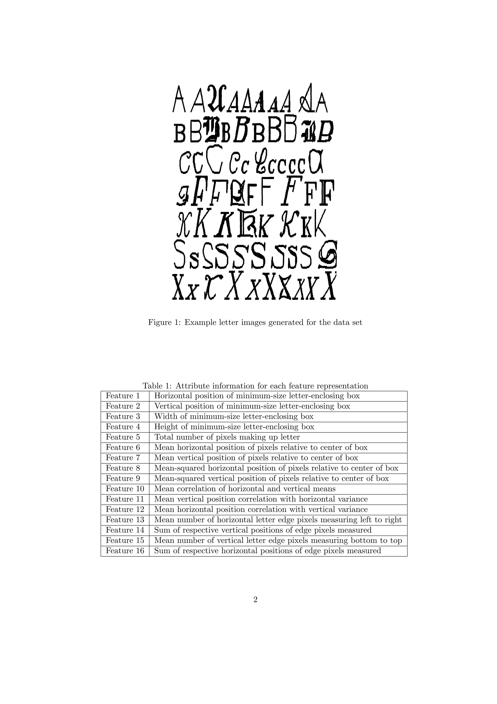
For the purpose of generating the data set an algorithm was created whose output would be an English
capital letter uniformly drawn from the letters of alphabet, randomly selected among 20 different fonts.
The fonts included five stroke styles (Simplex, Duplex, Triplex, Complex and Gothic) and six letter styles
(Block, Script, Italic, English, Italian and German). To further complicate the generated images, each letter
underwent a random distortion process including vertical and horizontal warping, linear magnification and
changes to the aspect ratio. Examples of the resulting images from the data set are shown in Figure 1.
The algorithm produced 20,000 unique letter images. Each image was converted into 16 primitive nu-
merical attributes, each values as a normalized 4-bit number with an integer value ranged from 0 through
15. The attributes used to construct the 16 features are detailed in Table 1. An example of the final data
points extracted from the data set is displayed in Figure 2.
For the purpose of this study we divided the data set of 20,000 letter images into two sets. To develop
the different models we allocated the first 16,000 letters as training data. The training data was divided
into 13,600 training images and 2,400 validation images for algorithms which required validation processes.
The remaining 4,000 letter images for used for testing. We further developed a z-score of the features and
replaced the letter labels with respective respective integers such that,
A = 1, B = 2, .., Z = 26. (1)
This label replacement was done for programming convenience. It should be noted that numerical closeness
between two letters does not represent letters that are close are similar to each other. This should be kept in
mind when using models that use regression analysis for classification. The concept of being close numerically
does not represent closeness between classes. Algorithms may favor numerically close letters, although there
is no real comparable basis for this consideration. Efforts were made in this project to use the algorithms in
a way which avoided this issue.
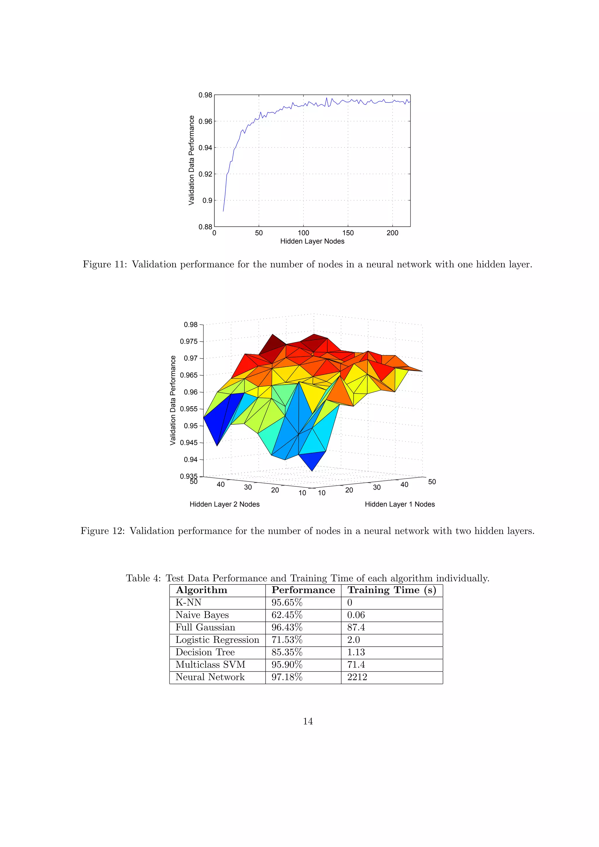
1](https://image.slidesharecdn.com/960ce3ee-ba97-457d-8cc4-562e4cb7feae-150123141040-conversion-gate01/75/FinalReportFoxMelle-1-2048.jpg)
![X,4,9,5,6,5,7,6,3,5,6,6,9,2,8,8,8
H,3,3,4,1,2,8,7,5,6,7,6,8,5,8,3,7
L,2,3,2,4,1,0,1,5,6,0,0,6,0,8,0,8
H,3,5,5,4,3,7,8,3,6,10,6,8,3,8,3,8
E,2,3,3,2,2,7,7,5,7,7,6,8,2,8,5,10
Y,5,10,6,7,6,9,6,6,4,7,8,7,6,9,8,3
H,8,12,8,6,4,9,8,4,5,8,4,5,6,9,5,9
Q,5,10,5,5,4,9,6,5,6,10,6,7,4,8,9,9
M,6,7,9,5,7,4,7,3,5,10,10,11,8,6,3,7
E,4,8,5,6,4,7,7,4,8,11,8,9,2,9,5,7
N,6,11,8,8,9,5,8,3,4,8,8,9,7,9,5,4
Y,8,10,8,7,4,3,10,3,7,11,12,6,1,11,3,5
W,4,8,5,6,3,6,8,4,1,7,8,8,8,9,0,8
O,6,7,8,6,6,6,6,5,6,8,5,8,3,6,5,6
N,4,4,4,6,2,7,7,14,2,5,6,8,6,8,0,8
H,4,8,5,6,5,7,10,8,5,8,5,6,3,6,7,11
O,4,7,5,5,3,8,7,8,5,10,6,8,3,8,3,8
N,4,8,5,6,4,7,7,9,4,6,4,6,3,7,3,8
H,4,9,5,6,2,7,6,15,1,7,7,8,3,8,0,8
Figure 2: Example Data extracted from data set
3 Methodology
The following subsections summarize the different algorithms that we used for letter classification and how
they were applied to our problem. Generally the models had 16 input dimensions, the features, and had an
output representing either the chosen letter or a decision on the comparison between letters. Understanding
of these algorithms was assisted by [2].
3.1 k-Nearest Neighbors
The k-Nearest Neighbors algorithm is a discriminative classifier that uses a deterministic association to
distinguish the data points. The output label for a test letter is a class membership determined by a
majority vote of its k closest neighbors in the feature space by Euclidean distance. The performance is
optimized by determining what value k of nearest neighbors which performs best on the validation data. A
k too large includes too much distant and irrelevant data, while a k too small risks misclassifications due to
noise.
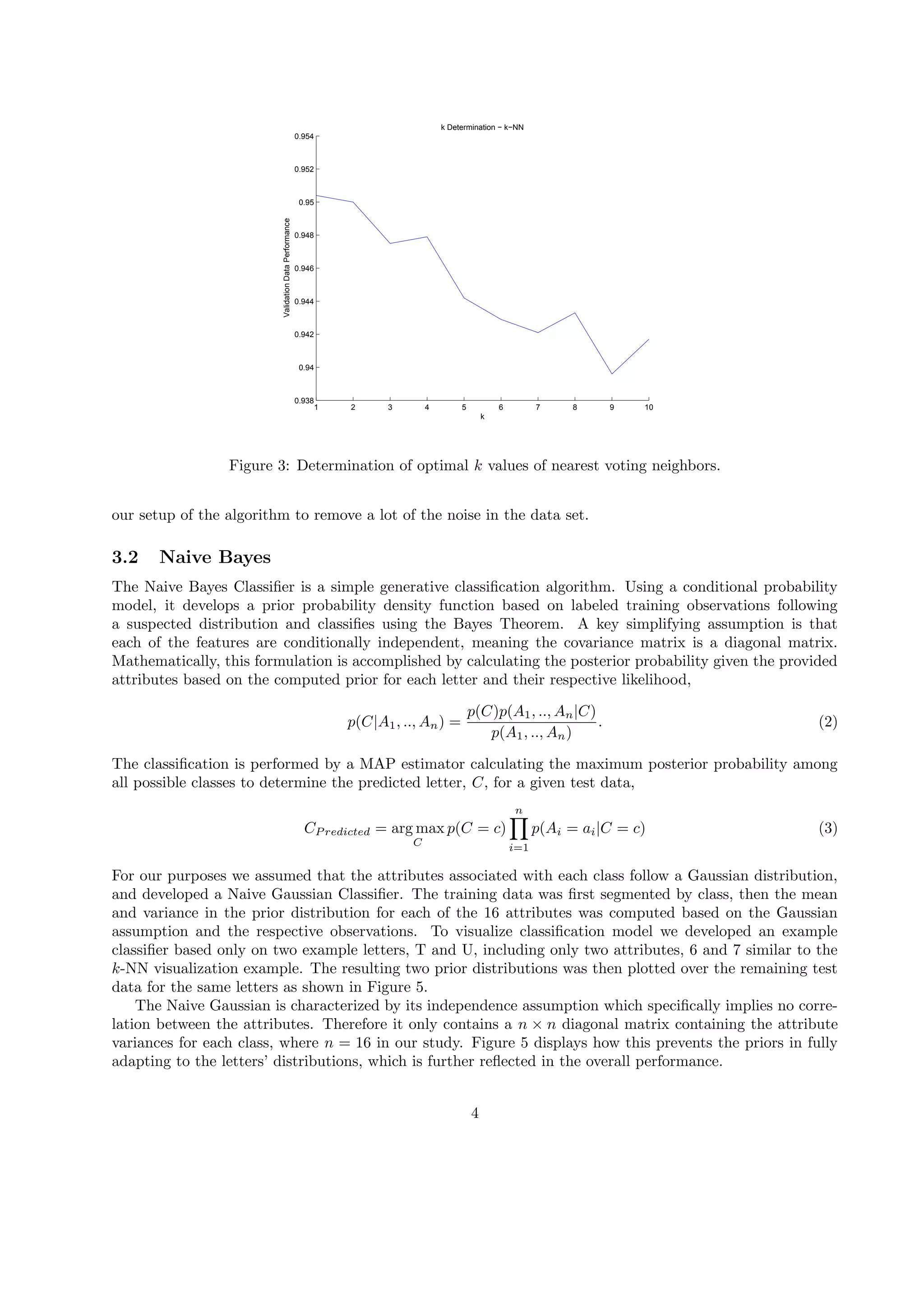
The graph of validation performance with respect to different k values is shown in Figure 3. The best
result was achieved with letting only one nearest neighbor vote, k = 1. This result is line with the fact that
the features are normalized to 4-bit values which limits the potential possibilities in the feature space and
leads to a lot of the data set thereby overlapping. Classifying a given test image based on only the majority
of letters having the same feature value may therefore be sufficient.
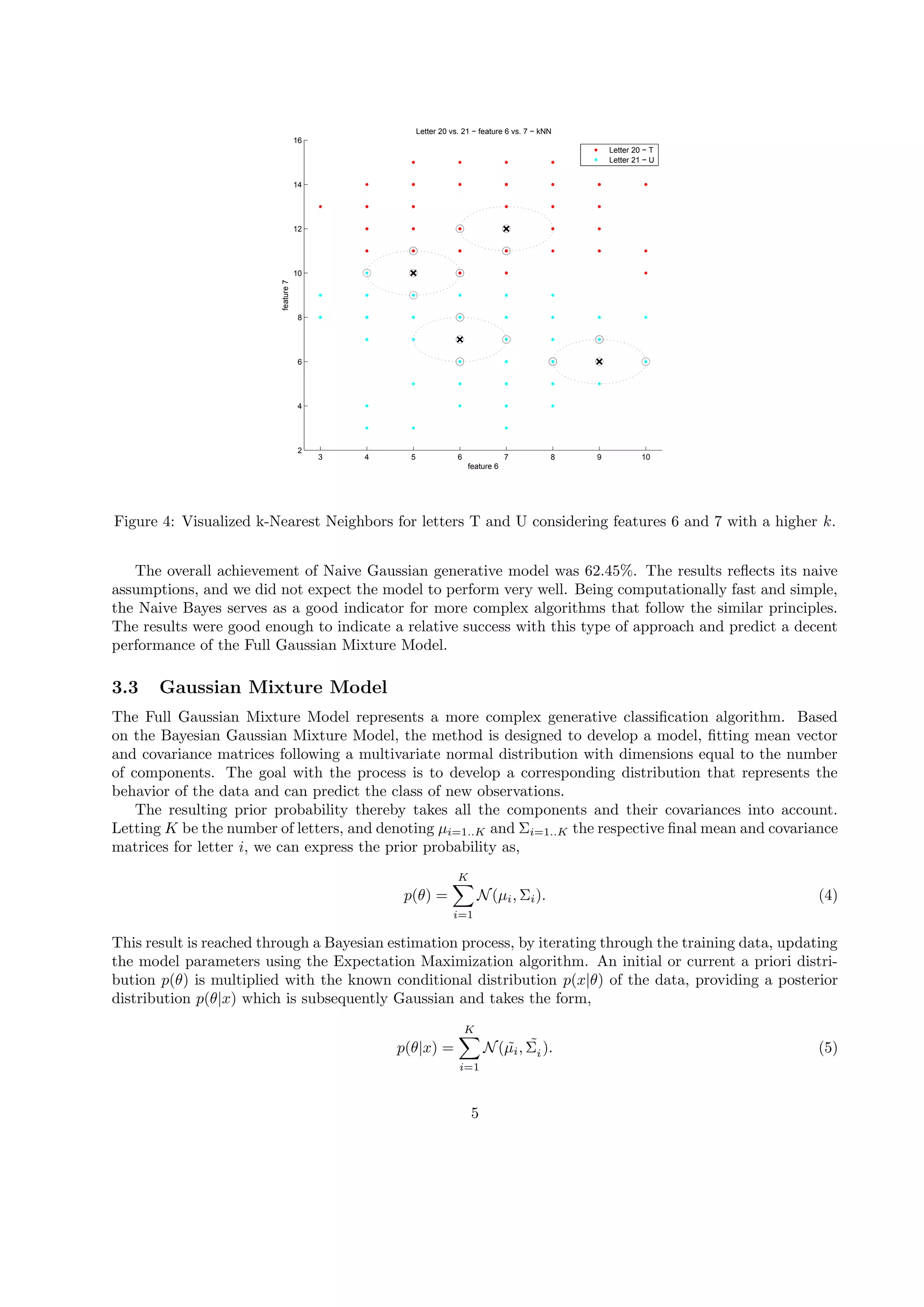
To visualize the classification process we extracted two letter examples, T and U from the training data
set, with two of their features (6 and 7) in Figure 4. On this data we added two test letters of each class
and classified them by a higher number of neighbors to visualize the voting process. As our k determination
process concluded with k = 1 for optimal results, our output will in reality only take in account the letters
having obtained the same value for the majority vote. It should be noted that this classification appears to
perform relatively poorly. That is due to the fact that we only used 2 features for simple visualization. The
full 16 dimensional feature space with all 26 letters would be impossible to illustrate.
The overall performance of the k-Nearest Neighbor Algorithm on the test data was 95.65%. This over
adequate achievement can be due to the sparsely ranged values of the attributes which enables us through
3](https://image.slidesharecdn.com/960ce3ee-ba97-457d-8cc4-562e4cb7feae-150123141040-conversion-gate01/75/FinalReportFoxMelle-3-2048.jpg)
![0 2 4 6 8 10 12 14 16
0
2
4
6
8
10
12
14
16
feature 6
feature7
Letter 20 vs. 21 − feature 6 vs. 7 − Full Gaussian
Letter 20 − T
Letter 21 − U
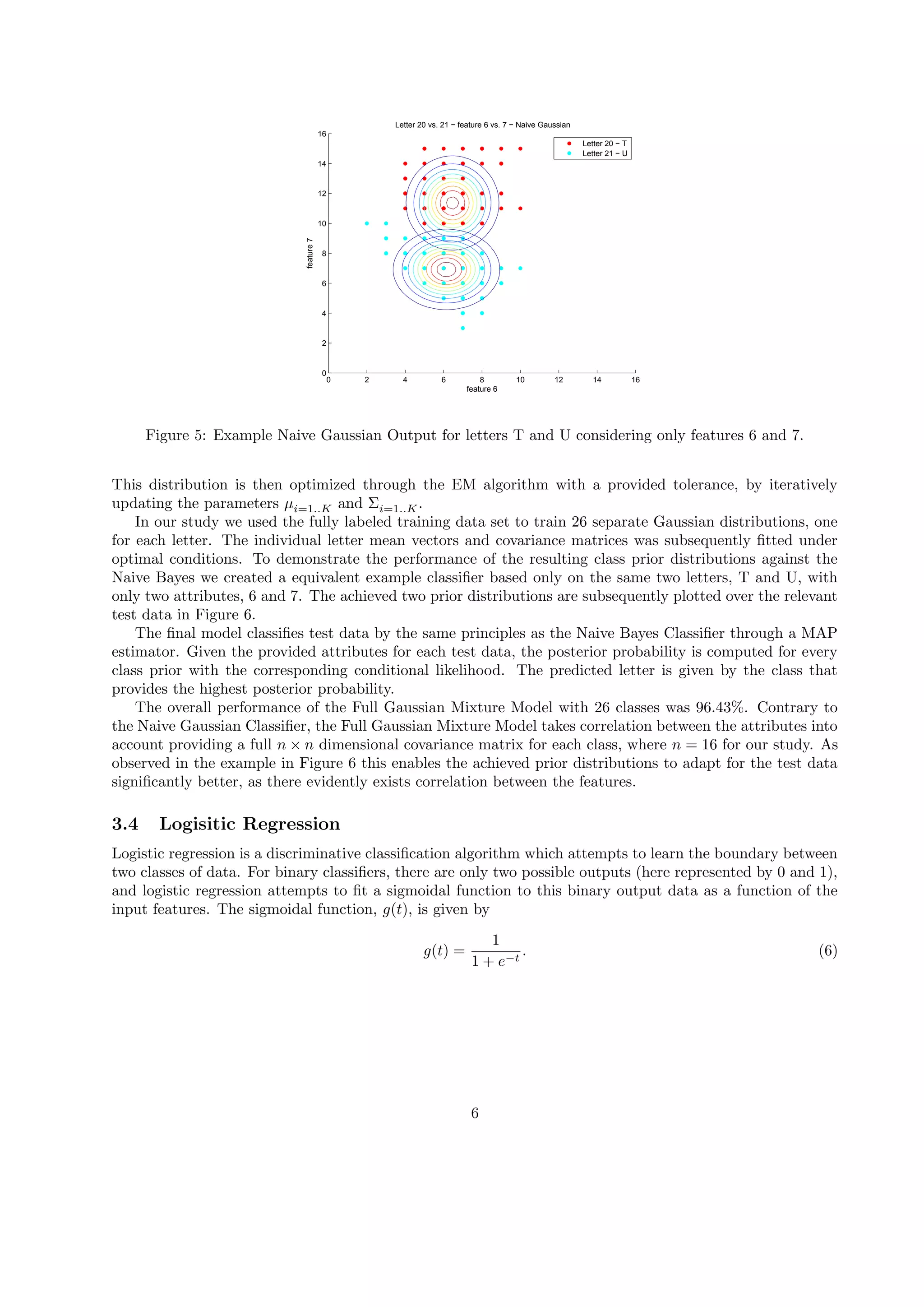
Figure 6: Example Full Gaussian Mixture Output for letters T and U considering only features 6 and 7.
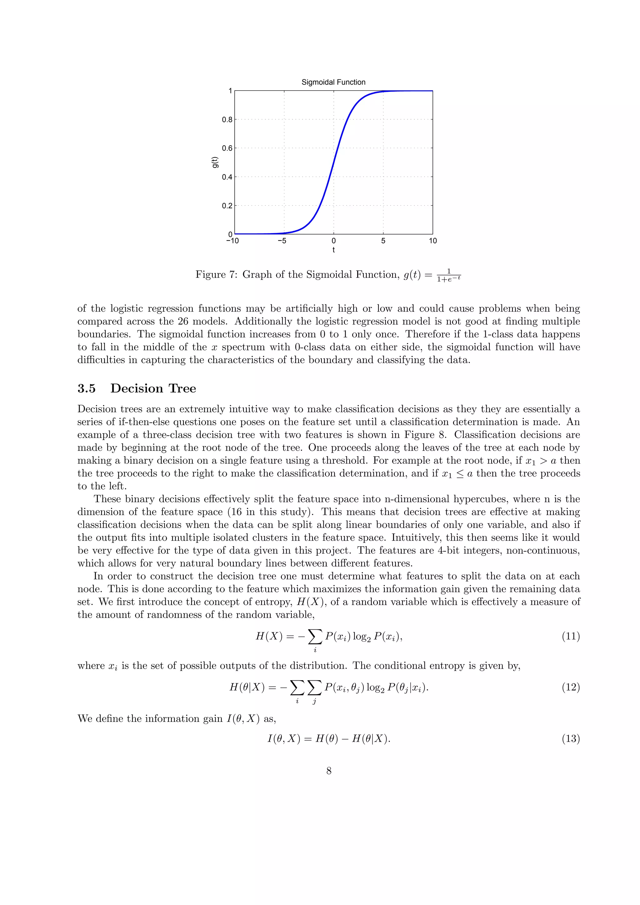
An example of the sigmoidal function is shown in Figure 7. Since the range of the sigmoidal function is
[0, 1],we can use it to represent the a posteriori probability p(θ|x) for the two classes as,
p(θ = 0|x) = g(wT
x) =
1
1 + e−wT x
, (7)
p(θ = 1|x) = 1 − g(wT
x) =
e−wT
x
1 + e−wT x
. (8)
The mathematical objective of using Logistic Regression as a binary classifier is to determine the vector w.
This is determined using the log-likelihood function. Given n labeled data points, {(X1, θ1), . . . , (Xn, θn)},
the log-likelihood function, l(x) is given by,
l(x) =
n∑
i=1
θi ln(1 − g(wT
xi)) + (1 − θi) ln(g(wT
xi)) (9)
=
n∑
i=1
θiwT
xi − ln(1 + ewT
xi
) (10)
We can differentiate this log-likelihood with respect to w, equate to zero to find the maximum, and solve for
the maximizing value of w using gradient descent.
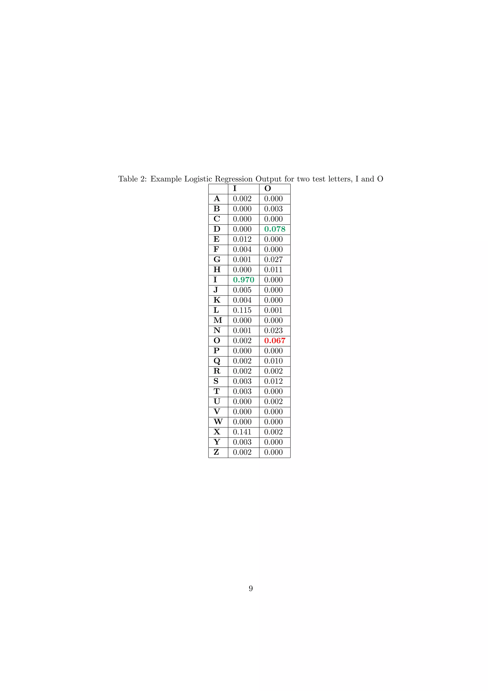
However logistic regression is a binary classifier and the Letter Recognition data set has 26 classes. To
account for this we create 26 different binary classifiers, each comparing an individual letter (denoted class
1) to all the remaining letters (denoted class 0). The determined letter corresponds to the maximum value of
the output of each of the logistic regression functions. An example of the output for two test letter examples,
I and O is shown in Table 2. The letter I is correctly classified with the logistic regression outputting a value
close to 1 for I and close to 0 for every other letter. However for the given test letter O, the features result
in an output close to 0 for every logistic regression output and the letter is misclassified as a D.
The overall classification performance of the logistic regression algorithm on the test data was 71.53%.
One of the weaknesses of the algorithm is that the 26 models for each letter are derived independently and
the output values are therefore not directly comparable. Some letters may be further away from the rest
of the letters than others and therefore the boundaries for different models and the area of change in the
resulting sigmoidal function from 0 to 1 will vary in terms of its width. Therefore output values from some
7](https://image.slidesharecdn.com/960ce3ee-ba97-457d-8cc4-562e4cb7feae-150123141040-conversion-gate01/75/FinalReportFoxMelle-7-2048.jpg)
![Table 3: Example Multiclass Support Vector Machine Output for two test letters, I and O
I O
A 3 3
B 1 11
C 6 20
D 11 23
E 3 6
F 15 9
G 10 21
H 19 20
I 25 0
J 12 5
K 21 13
L 7 4
M 23 17
N 17 19
O 3 25
P 21 18
Q 18 24
R 9 14
S 21 18
T 10 8
U 12 12
V 3 2
W 16 9
X 10 8
Y 23 12
Z 6 4
-1 plane
+1 plane
jkε ε
Figure 10: Example Support Vector Machine with boundaries [3].
12](https://image.slidesharecdn.com/960ce3ee-ba97-457d-8cc4-562e4cb7feae-150123141040-conversion-gate01/75/FinalReportFoxMelle-12-2048.jpg)
![Table 8: Amount of shared overlap of misclassifications among the algorithms in the Weak and Strong hybrid
models.
Weak Models Strong Models
Algorithm # Misclassifications Overlap Algorithm # Misclassifications Overlap >3
Naive Bayes 1502
306
k-NN 174
77
Logistic Regression 1139 Full Gaussian 149
Decision Tree 586 SVM 164
Neural Network 119
in misclassifications among the individual algorithms in both the weak and strong hybrid models. Compared
to the best performing model in each situation, there is a large amount of overlap in the misclassifications
between the models. This leaves very few test cases where fixed classifications could be expected. Generally
hybrid models such as these tend to work best with a larger amount of weaker models, since there are more
possible votes and more room for improvement.
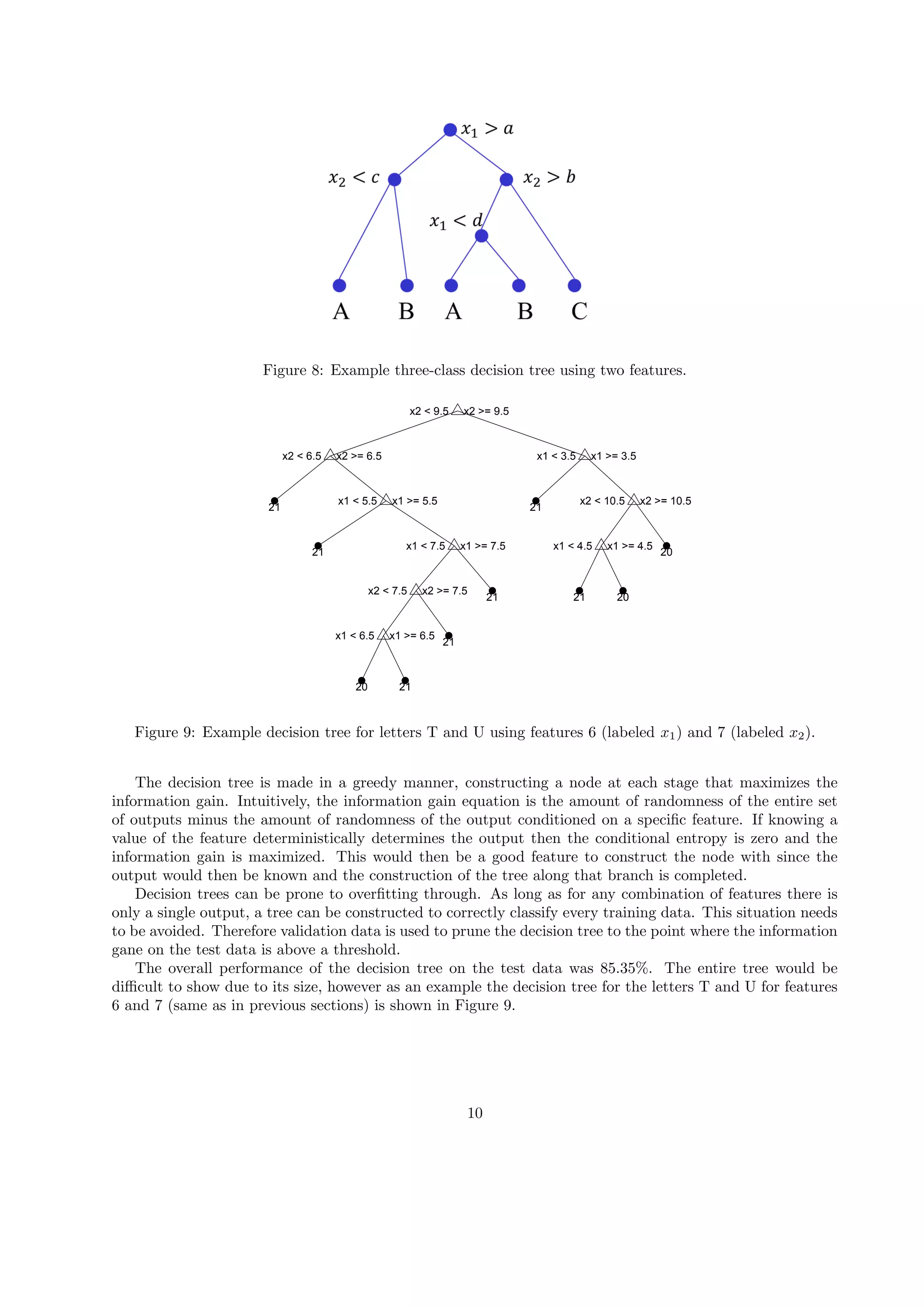
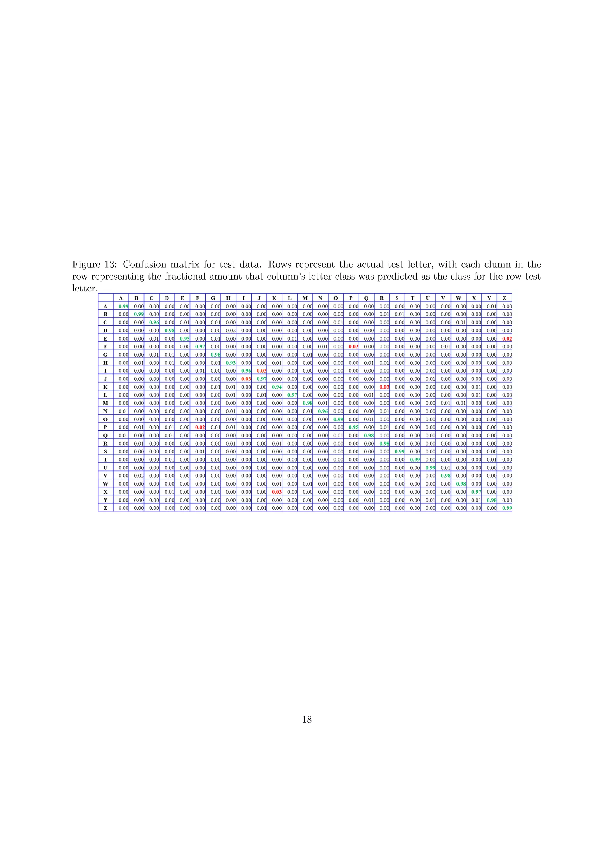
3.10 Final Confusion Matrix
We present the confusion matrix for the best performing performance-weighted vote in Figure 13. Highlighted
in green are the correct predictions for each letter and highlighted in red are some of the interesting and
most frequent letter misclassifications. We perform worst on the letter H, correctly predicting it only 93%
of the time. Some misclassifications include mistaking the letter I for J and vice-versa. It should be noted
that the confusion matrix is not symmetric, meaning that even though one letter is often misclassified as a
second it does not mean that the second letter gets misclassified as the first, although that is not an unusual
scenario. This is because some of the letters can be better discriminated than others, and some are closer
to the general distribution of the remaining letters than others. For example the letter K is misclassified as
an R 3% of the time, while the letter R is misclassified as the letter K only 1% of the time.
In general this confusion matrix matches up well with our general intuition of how the classifications would
perform. Letters that are most frequently misclassified as others tend to have a significant resemblance to
the human eye.
4 Conclusions
We used seven different machine learning algorithms to classify letter images based on 16 predetermined
features. Our best performance was accomplished with a neural network at 97.18%. We were able to slightly
increase this result to 97.50%. using a voting scheme among many models. However the improvement with
the hybrid models was less than originally hoped for due to the already good performance from the original
models, as well as the nature of the data, in that the letters that were misclassified were often commonly
misclassified by most of the individual algorithms.
References
[1] P. W. Frey and D. J. Slate, “Letter recognition using holland-style adaptive classifiers,” Mach. Learn.,
vol. 6, pp. 161–182, Mar. 1991.
[2] C. M. Bishop, Pattern Recognition and Machine Learning (Information Science and Statistics). Secaucus,
NJ, USA: Springer-Verlag New York, Inc., 2006.
[3] Z.-B. Joseph, “10701 machine learning, neural network lecture slides,” 2012.
17](https://image.slidesharecdn.com/960ce3ee-ba97-457d-8cc4-562e4cb7feae-150123141040-conversion-gate01/75/FinalReportFoxMelle-17-2048.jpg)

- The document describes a study that used various machine learning algorithms to classify images of letters based on 16 extracted features. - The best performing algorithm was the Gaussian Mixture Model, which achieved 96.43% accuracy by modeling each letter as a Gaussian distribution and accounting for correlations between features. - The k-Nearest Neighbors algorithm achieved 95.65% accuracy when using only the single nearest neighbor for classification, while the Naive Bayes classifier achieved only 62.45% due to its strong independence assumptions.