Instrumentation And Control Systems 3rd Edition William Bolton
Instrumentation And Control Systems 3rd Edition William Bolton
Instrumentation And Control Systems 3rd Edition William Bolton
Instrumentation And Control Systems 3rd Edition William Bolton
Instrumentation And Control Systems 3rd Edition William Bolton
1.
Instrumentation And ControlSystems 3rd Edition
William Bolton download
https://ebookbell.com/product/instrumentation-and-control-
systems-3rd-edition-william-bolton-26846252
Explore and download more ebooks at ebookbell.com
2.
Here are somerecommended products that we believe you will be
interested in. You can click the link to download.
Instrumentation And Control Systems William Bolton
https://ebookbell.com/product/instrumentation-and-control-systems-
william-bolton-50542562
Instrumentation And Control Systems W Bolton Auth
https://ebookbell.com/product/instrumentation-and-control-systems-w-
bolton-auth-4411228
Instrumentation And Control Systems Documentation 2nd Frederick A
Meier
https://ebookbell.com/product/instrumentation-and-control-systems-
documentation-2nd-frederick-a-meier-4707130
Instrumentation And Control Systems Documentation Fred A Meier
Clifford A Meier
https://ebookbell.com/product/instrumentation-and-control-systems-
documentation-fred-a-meier-clifford-a-meier-4723758
3.
Instrumentation And ControlSystems Second Edition Second Edition
Bolton
https://ebookbell.com/product/instrumentation-and-control-systems-
second-edition-second-edition-bolton-5432040
Instrumentation And Control Systems Reddy
https://ebookbell.com/product/instrumentation-and-control-systems-
reddy-10953550
Successful Instrumentation And Control Systems Design Bkcdrom Michael
D Whitt
https://ebookbell.com/product/successful-instrumentation-and-control-
systems-design-bkcdrom-michael-d-whitt-2112458
Successful Instrumentation And Control Systems Design 2nd Ed Whitt
https://ebookbell.com/product/successful-instrumentation-and-control-
systems-design-2nd-ed-whitt-9951410
Successful Instrumentation And Control Systems Design Michael D Whitt
https://ebookbell.com/product/successful-instrumentation-and-control-
systems-design-michael-d-whitt-1208262
Contents
Preface ix
Acknowledgement xiii
1.Measurement Systems 1
1.1 Introduction 1
1.1.1 Systems 1
1.2 Instrumentation Systems 2
1.2.1 The Constituent Elements of an
Instrumentation System 2
1.3 Performance Terms 4
1.3.1 Resolution, Accuracy, and Error 4
1.3.2 Range 6
1.3.3 Precision, Repeatability, and Reproducibility 7
1.3.4 Sensitivity 7
1.3.5 Stability 8
1.3.6 Dynamic Characteristics 9
1.4 Dependability 9
1.4.1 Reliability 10
1.5 Requirements 11
1.5.1 Calibration 12
1.5.2 Safety Systems 13
Problems 14
2. Instrumentation System Elements 17
2.1 Introduction 18
2.2 Displacement Sensors 18
2.2.1 Potentiometer 18
2.2.2 Strain-Gauged Element 19
2.2.3 Capacitive Element 20
2.2.4 Linear Variable Differential Transformer 21
2.2.5 Optical Encoders 21
2.2.6 Moiré Fringes 22
2.2.7 Optical Proximity Sensors 23
2.2.8 Mechanical Switches 24
2.2.9 Capacitive Proximity Sensor 25
2.2.10 Inductivity Proximity Sensor 26
2.3 Speed Sensors 26
2.3.1 Optical Methods 26
2.3.2 Incremental Encoder 26
2.3.3 Tachogenerator 26
2.4 Fluid Pressure Sensors 26
2.4.1 Diaphragm Sensor 27
2.4.2 Piezoelectric Sensor 28
2.4.3 Bourdon Tube 28
2.5 Fluid Flow 29
2.5.1 Differential Pressure Methods 29
2.5.2 Turbine Meter 31
2.5.3 Ultrasonic Time of Flight Flow Meter 32
2.5.4 Vortex Flow Rate Method 32
2.5.5 Coriolis Flow Meter 33
2.6 Liquid Level 33
2.6.1 Floats 34
2.6.2 Displacer Gauge 34
2.6.3 Differential Pressure 34
2.6.4 Load Cell 34
2.6.5 Electrical Conductivity Level Indicator 35
2.6.6 Capacitive Level Indicator 35
2.6.7 Ultrasonic Level Gauge 35
2.6.8 Nucleonic Level Indicators 36
2.7 Temperature Sensors 36
2.7.1 Bimetallic Strips 36
2.7.2 Liquid in Glass Thermometers 36
2.7.3 Resistance Temperature Detectors (RTDs) 36
2.7.4 Thermistors 37
2.7.5 Thermocouples 37
2.7.6 Thermodiodes and Transistors 40
2.7.7 Pyrometers 40
2.8 Sensor Selection 41
2.9 Signal Processing 42
2.9.1 Resistance to Voltage Converter 42
2.9.2 Temperature Compensation 45
2.9.3 Thermocouple Compensation 45
2.9.4 Protection 47
2.9.5 Analogue-to-Digital Conversions 47
2.9.6 Digital-to-Analogue Conversions 50
2.9.7 Microcontroller Systems 51
2.9.8 Op-Amps 52
2.9.9 Pressure-to-Current Converter 56
2.10 Signal Transmission 56
2.10.1 Noise 59
2.11 Smart Systems 60
2.11.1 MEMS 61
2.12 Data Presentation Element 62
2.12.1 Indicator 62
2.12.2 Illuminative Displays 62
2.12.3 Graphical User Interface (GUI) 64
2.12.4 Data Loggers 64
2.12.5 Printers 65
Problems 66
v
9.
3. Measurement CaseStudies 71
3.1 Introduction 71
3.2 Case Studies 72
3.2.1 A Temperature Measurement 72
3.2.2 An Absolute Pressure Measurement 73
3.2.3 Detection of the Angular Position of a
Shaft 74
3.2.4 Air Flow Rate Determination 74
3.2.5 Fluid Level Monitoring 75
3.2.6 Measurement of Relative Humidity 75
3.2.7 Dimension Checking 76
3.2.8 Temperature of a Furnace 77
3.2.9 Automobile Tyre Pressure Monitoring 77
3.2.10 Control System Sensors with Automobiles 77
3.3 Data Acquisition Systems 78
3.3.1 Data Acquisition Software 80
3.3.2 Data Loggers 80
3.4 Testing 80
3.4.1 Maintenance 80
3.4.2 Common Faults 81
Problems 82
4. Control Systems 85
4.1 Introduction 85
4.2 Control Systems 86
4.2.1 Open- and Closed-Loop Control 87
4.3 Basic Elements 89
4.3.1 Basic Elements of a Closed-Loop System 89
4.4 Case Studies 91
4.4.1 Control of the Speed of Rotation of a
Motor Shaft 91
4.4.2 Control of the Position of a Tool 92
4.4.3 Power Steering 92
4.4.4 Control of Fuel Pressure 93
4.4.5 Antilock Brakes 93
4.4.6 Thickness Control 94
4.4.7 Control of Liquid Level 95
4.4.8 Robot Gripper 95
4.4.9 Machine Tool Control 97
4.4.10 Fluid Flow Control 97
4.5 Discrete-Time Control Systems 98
4.6 Digital Control Systems 99
4.7 Hierarchical Control 100
Problems 101
5. Process Controllers 103
5.1 Introduction 103
5.1.1 Direct and Reverse Actions 104
5.1.2 Dead Time 104
5.1.3 Capacitance 104
5.2 On Off Control 104
5.2.1 Relays 106
5.3 Proportional Control 107
5.3.1 Proportional Band 107
5.3.2 Limitations of Proportional Control 109
5.4 Derivative Control 110
5.4.1 PD Control 110
5.5 Integral Control 112
5.5.1 PI Control 112
5.6 PID Control 114
5.6.1 PID Process Controller 116
5.7 Tuning 117
5.7.1 Process Reaction Tuning Method 118
5.7.2 Ultimate Cycle Tuning Method 120
5.7.3 Quarter Amplitude Decay 121
5.7.4 Lambda Tuning 121
5.7.5 Software Tools 121
5.7.6 Adaptive Controllers 122
5.8 Digital Systems 122
5.8.1 Embedded Systems 123
5.9 Fuzzy Logic Control 124
5.9.1 Fuzzy Logic 124
5.9.2 Fuzzy Logic Control Systems 126
5.9.3 Fuzzy Logic Controller 127
5.9.4 Fuzzy Logic Tuning of PID Controllers 130
5.10 Neural Networks 130
5.10.1 Neural Networks for Control 132
Problems 133
6. Correction Elements 137
6.1 Introduction 137
6.1.1 The Range of Actuators 138
6.2 Pneumatic and Hydraulic Systems 138
6.2.1 Current to Pressure Converter 138
6.2.2 Pressure Sources 138
6.2.3 Control Valves 139
6.2.4 Actuators 140
6.3 Directional Control Valves 141
6.3.1 Sequencing 143
6.3.2 Shuttle Valve 145
6.4 Flow Control Valves 146
6.4.1 Forms of Plug 147
6.4.2 Rangeability and Turndown 149
6.4.3 Control Valve Sizing 149
6.4.4 Valve Positioners 151
6.4.5 Other Forms of Flow Control Valves 151
6.4.6 Fail-Safe Design 152
6.5 Motors 152
6.5.1 D.C. Motors 152
6.5.2 Brushless Permanent Magnet D.C. Motor 154
6.5.3 Stepper Motor 154
6.6 Case Studies 159
6.6.1 A Liquid Level Process Control System 159
6.6.2 Milling Machine Control System 159
6.6.3 A Robot Control System 159
Problems 160
vi CONTENTS
10.
7. PLC Systems165
7.1 Introduction 165
7.2 Logic Gates 166
7.2.1 Field-Programmable Gate Arrays 169
7.3 PLC System 170
7.4 PLC Programming 171
7.4.1 Logic Gates 173
7.4.2 Latching 174
7.4.3 Internal Relays 174
7.4.4 Timers 175
7.4.5 Counters 176
7.5 Testing and Debugging 178
7.6 Case Studies 179
7.6.1 Signal Lamp to Monitor Operations 179
7.6.2 Cyclic Movement of a Piston 179
7.6.3 Sequential Movement of Pistons 179
7.6.4 Central Heating System 181
Problems 182
8. System Models 189
8.1 Introduction 189
8.1.1 Static Response 189
8.1.2 Dynamic Response 189
8.2 Gain 190
8.2.1 Gain of Systems in Series 191
8.2.2 Feedback Loops 191
8.3 Dynamic Systems 193
8.3.1 Mechanical Systems 193
8.3.2 Rotational Systems 194
8.3.3 Electrical Systems 196
8.3.4 Thermal Systems 198
8.3.5 Hydraulic Systems 200
8.4 Differential Equations 202
8.4.1 First-Order Differential Equations 202
8.4.2 Second-Order Differential Equations 204
8.4.3 System Identification 205
Problems 206
9. Transfer Function 209
9.1 Introduction 209
9.2 Transfer Function 210
9.2.1 Transfer Function 211
9.2.2 Transfer Functions of Common System
Elements 212
9.2.3 Transfer Functions and Systems 213
9.3 System Transfer Functions 214
9.3.1 Systems in Series 214
9.3.2 Systems with Feedback 215
9.4 Block Manipulation 216
9.4.1 Blocks in Series 217
9.4.2 Moving Takeoff Points 217
9.4.3 Moving a Summing Point 217
9.4.4 Changing Feedback and Forward Paths 217
9.5 Multiple Inputs 220
9.6 Sensitivity 221
9.6.1 Sensitivity to Changes in Parameters 221
9.6.2 Sensitivity to Disturbances 223
Problems 223
10. System Response 227
10.1 Introduction 227
10.2 Inputs 227
10.3 Determining Outputs 228
10.3.1 Partial Fractions 230
10.4 First-Order Systems 233
10.4.1 First-Order System Parameters 235
10.5 Second-Order Systems 237
10.5.1 Second-Order System Parameters 240
10.6 Stability 245
10.6.1 The s Plane 246
10.7 Steady-State Error 250
Problems 252
11. Frequency Response 257
11.1 Introduction 257
11.1.1 Sinusoidal Signals 258
11.1.2 Complex Numbers 258
11.2 Sinusoidal Inputs 260
11.2.1 Frequency Response Function 260
11.2.2 Frequency Response for First-Order
Systems 262
11.2.3 Frequency Response for Second-Order
Systems 264
11.3 Bode Plots 265
11.3.1 Transfer Function a Constant K 266
11.3.2 Transfer Function 1/sn
266
11.3.3 Transfer Function sm
267
11.3.4 Transfer Function 1/(1 1 τs) 267
11.3.5 Transfer Function (1 1 τs) 269
11.3.6 Transfer Function
ωn
2
/(s2
1 2ζωns 1 ωn
2
) 270
11.3.7 Transfer Function
(s2
1 2ζωns 1 ωn
2
)/ωn
2
272
11.4 System Identification 274
11.5 Stability 276
11.5.1 Stability Measures 277
11.6 Compensation 278
11.6.1 Changing the Gain 278
11.6.2 Phase-Lead Compensation 280
11.6.3 Phase-Lag Compensation 281
Problems 283
12. Nyquist Diagrams 287
12.1 Introduction 287
12.2 The Polar Plot 287
12.2.1 Nyquist Diagrams 289
12.3 Stability 290
12.4 Relative Stability 292
Problems 293
vii
CONTENTS
11.
13. Control Systems297
13.1 Introduction 297
13.2 Controllers 298
13.2.1 Proportional Steady-State Offset 300
13.2.2 Disturbance Rejection 301
13.2.3 Integral Wind-Up 301
13.2.4 Bumpless Transfer 302
13.3 Frequency Response 302
13.4 Systems with Dead Time 303
13.5 Cascade Control 305
13.6 Feedforward Control 306
13.7 Digital Control Systems 307
13.7.1 The z-Transform 309
13.7.2 The Digital Transfer Function G(z) 311
13.7.3 PID Controller 314
13.7.4 Software Implementation of PID
Control 317
13.8 Control Networks 317
13.8.1 Data Transmission 318
13.8.2 Networks 319
13.8.3 Control Area Network (CAN) 320
13.8.4 Automated Assembly Lines 321
13.8.5 Automated Process Plant Networks 321
13.8.6 PLC Networks 323
13.8.7 Supervisory Control and Data
Acquisition (SCADA) 325
13.8.8 The Common Industrial Protocol
(CIP) 326
13.8.9 Security Issues 326
Problems 327
Answers 329
Appendix A: Errors 341
Appendix B: Differential Equations 347
Appendix C: Laplace Transform 353
Appendix D: The z-Transform 361
Index 367
viii CONTENTS
12.
Preface
This book providesa first-level introduction to instrumentation and control engineering and
as such is suitable for the BTEC units of Industrial Process Controllers and Industrial Plant and
Process Control for the National Certificates and Diplomas in Engineering, and the unit Control
Systems and Automation for the Higher National Certificates and Diplomas in Engineering and
also providing a basic introduction to instrumentation and control systems for undergradu-
ates. The book aims to give an appreciation of the principles of industrial instrumentation and
an insight into the principles involved in control engineering.
The book integrates actual hardware with theory and analysis, aiming to make the mathe-
matics of control engineering as readable and approachable as possible.
STRUCTURE OF THE BOOK
The book has been designed to give a clear exposition and guide readers through the princi-
ples involved in the design and use of instrumentation and control systems, reviewing back-
ground principles where necessary. Each chapter includes worked examples, multiple-choice
questions and problems; answers are supplied to all questions and problems. There are
numerous case studies in the text indicating applications of the principles.
PERFORMANCE OUTCOMES
The following indicate the outcomes for which each chapter has been planned. At the end
of the chapters the reader should be able to:
Chapter 1: Measurement systems
Read and interpret performance terminology used in the specifications of
instrumentation.
Chapter 2: Instrumentation system elements
Describe and evaluate sensors commonly used with instrumentation used in the
measurement of position, rotational speed, pressure, flow, liquid level, temperature and
the detection of the presence of objects.
Describe and evaluate methods used for signal processing and display.
Chapter 3: Measurement case studies
Explain how system elements are combined in instrumentation for some commonly
encountered measurements.
ix
13.
Chapter 4: Controlsystems
Explain what is meant by open and closed-loop control systems, the differences in
performance between such systems.
Explain the principles involved in some simple examples of open and closed-loop control
systems.
Describe the basic elements of digital control systems.
Chapter 5: Process controllers
Describe the function and terminology of a process controller and the use of two-step,
proportional, derivative and integral control laws.
Explain PID control and how such a controller can be tuned.
Explain what is meant by fuzzy logic and how it can be used for control applications.
Explain what is meant by artificial neural networks and how they can be used for control
applications.
Chapter 6: Correction elements
Describe common forms of correction/regulating elements used in control systems.
Describe the forms of commonly used pneumatic/hydraulic and electric correction
elements.
Chapter 7: PLC systems
Describe the functions of logic gates and the use of truth tables.
Describe the basic elements involved with PLC systems.
Devise programs to enable PLCs to carry out simple control tasks.
Chapter 8: System models
Explain how models for physical systems can be constructed in terms of simple building
blocks.
Chapter 9: Transfer function
Define the term transfer function and explain how it is used to relate outputs to inputs for
systems.
Use block diagram simplification techniques to aid in the evaluation of the overall
transfer function of a number of system elements.
Chapter 10: System response
Use Laplace transforms to determine the response of systems to common forms of inputs.
Use system parameters to describe the performance of systems when subject to a step
input.
Analyse systems and obtain values for system parameters.
Explain the properties determining the stability of systems.
Derive the steady-state error for a basic closed-loop control system.
Chapter 11: Frequency response
Explain how the frequency response function can be obtained for a system from its
transfer function.
Construct Bode plots from a knowledge of the transfer function.
Use Bode plots for first and second-order systems to describe their frequency response.
Use practically obtained Bode plots to deduce the form of the transfer function of a
system.
Compare compensation techniques.
x PREFACE
14.
Chapter 12: Nyquistdiagrams
Draw and interpret Nyquist diagrams.
Chapter 13: Control systems
Explain the reasons for the choices of P, PI, or PID controllers.
Explain the effect of dead time on the behaviour of a control system.
Explain the uses of cascade control and feedforward control.
Explain the principles of digital control systems and the use of the z-transform to analyse
them.
Describe the principles involved in control networks.
Describe the principles involved in Fieldbus.
Describe the principles of CAN, SCADA, DSC and CIP control networks.
Identify the issues involved in maintaining a secure system.
SOFTWARE TOOLS
Details of programs and methods suitable for their development have not been included
in this book. It was felt to be more appropriate to leave such development to more special-
ist texts such as MATLAB and SIMULINK for Engineers by Agam Kumar Tyagi (Oxford
Higher Education 2011), A Guide to MATLAB: For Beginners and Experienced Users by
B. R. Hunt and R. L. Lipsman (Cambridge University Press 2014), Hands-On Introduction
to LabView for Scientists and Engineers by John Essick (Oxford University Press 2012), and
Labview for Everyone: Graphical Programming Made Easy and Fun by Jeffrey Travis
(Prentice Hall, 2006).
CHANGES FOR THE 3RD EDITION
The major changes introduced to the third edition are a discussion of dependability that has
been included in Chapter 1, the discussion of smart systems extended and an introduction to
radio telemetry for data transmission. A discussion of interactive and non-interactive forms of
PID control and integrator windup has been added to Chapter 5, and it also now includes a
revised discussion of steady-state error and fuzzy logic and artificial neural networks for con-
trol applications. Chapter 10 extends the discussion of the steady-state error. Chapter 13
extends the discussion of the z-transform and bus systems used with control networks, intro-
ducing the HART Communication Protocol, Fieldbus and CIP control networks, and also
extends the discussion of security issues. An appendix has been included on the basic features
of the z-transform.
W. Bolton
xi
PREFACE
15.
Acknowledgement
I am gratefulto all those who reviewed the previous edition and made very helpful
suggestions for this new edition.
xiii
mechanical energy, thoughyou might consider there is also an output of waste heat. The interest is in the rela-
tionship between the output and the input rather than the internal science of the motor and how it operates. It is
convenient to think of the system in the box operating on the input to produce the output. Thus, in the case of an
amplifier system (Figure 1.3) we can think of the system multiplying the input V by some factor G, i.e. the ampli-
fier gain, to give the output GV.
Often we are concerned with a number of linked systems. For example, we might have a CD player system
linked to an amplifier system, which, in turn, is linked to a loudspeaker system. We can then draw this as three
interconnected boxes (Figure 1.4) with the output from one system becoming the input to the next system. In draw-
ing a system as a series of interconnected blocks, it is necessary to recognise that the lines drawn to connect boxes
indicate a flow of information in the direction indicated by the arrow and not necessarily physical connections.
1.2 INSTRUMENTATION SYSTEMS
The purpose of an instrumentation system used for making measurements is to give the user a numerical value
corresponding to the variable being measured. Thus a thermometer may be used to give a numerical value for
the temperature of a liquid. We must, however, recognise that, for a variety of reasons, this numerical value may
not actually be the true value of the variable. Thus, in the case of the thermometer, there may be errors due to
the limited accuracy in the scale calibration, or reading errors due to the reading falling between two scale mark-
ings, or perhaps errors due to the insertion of a cold thermometer into a hot liquid, lowering the temperature of
the liquid and so altering the temperature being measured. We thus consider a measurement system to have an
input of the true value of the variable being measured and an output of the measured value of that variable
(Figure 1.5). Figure 1.6 shows some examples of such instrumentation systems.
An instrumentation system for making measurements has an input of the true value of the variable being mea-
sured and an output of the measured value. This output might be then used in a control system to control the
variable to some set value.
1.2.1 The Constituent Elements of an Instrumentation System
An instrumentation system for making measurements consists of several elements which are used to carry out
particular functions. These functional elements are:
1. Sensor
This is the element of the system which is effectively in contact with the process for which a variable is
being measured and gives an output which depends in some way on the value of the variable and which can
System
System boundary
Environment
Outputs
Inputs
FIGURE 1.1 A system.
Electric
motor
Input
Electrical
energy
Output
Mechanical
energy
FIGURE 1.2 Electric motor system.
Input Output
Amplifier
Gain G
V GV
FIGURE 1.3 Amplifier system.
CD player Amplifier
Input
A CD Electrical
signals
Bigger
electrical
signals
Output from CD player
Input to amplifier
Output from amplifier
Input to speaker
Output
Sound
Speaker
FIGURE 1.4 Interconnected systems.
2 1. MEASUREMENT SYSTEMS
INSTRUMENTATION AND CONTROL SYSTEMS
18.
be used bythe rest of the measurement system to give a value to it. For example, a thermocouple is a sensor
which has an input of temperature and an output of a small e.m.f. (Figure 1.7A) which in the rest of the
measurement system might be amplified to give a reading on a meter. Another example of a sensor is a
resistance thermometer element which has an input of temperature and an output of a resistance change
(Figure 1.7B).
2. Signal processor
This element takes the output from the sensor and converts it into a form which is suitable for display or
onward transmission in some control system. In the case of the thermocouple this may be an amplifier to
make the e.m.f. big enough to register on a meter (Figure 1.8B). There often may be more than an item,
perhaps an element which puts the output from the sensor into a suitable condition for further processing and
then an element which processes the signal so that it can be displayed. The term signal conditioner is used for
an element which converts the output of a sensor into a suitable form for further processing. Thus in the case
of the resistance thermometer there might be a signal conditioner, such as a Wheatstone bridge, which
transforms the resistance change into a voltage change, then an amplifier to make the voltage big enough for
display (Figure 1.8B) or for use in a system used to control the temperature.
3. Data presentation
This presents the measured value in a form which enables an observer to recognise it (Figure 1.9). This may
be via a display, e.g. a pointer moving across the scale of a meter or perhaps information on a visual display
unit (VDU). Alternatively, or additionally, the signal may be recorded, e.g. in a computer memory, or
transmitted to some other system such as a control system.
Figure 1.10 shows how these basic functional elements form a measurement system.
Measurement
system
Input:
true value
of variable
Output:
measured
value of
variable
FIGURE 1.5 An instrumentation/measurement system.
Measurement
system
Input Output
Pressure Value for
the pressure
(A)
Measurement
system
Input Output
Value for
the speed
(B)
Speed
Measurement
system
Input Output
Value for
the flow rate
(C)
Flow rate
FIGURE 1.6 Examples of instrumentation
systems: (A) pressure measurement, (B) speed-
ometer, (C) flow rate measurement.
Sensor:
thermocouple
Input:
temperature
Output:
e.m.f.
(A)
Sensor:
resistance
element
Input:
temperature
Output:
resistance
change
(B)
FIGURE 1.7 Sensors: (A) thermocouple, (B) resistance
thermometer.
Amplifier
Input: Output:
small
e.m.f.
larger
voltage
Wheatstone
bridge
Amplifier
Input:
resistance
change
Voltage
change
Larger
voltage
change
(A) (B)
Output: FIGURE 1.8 Examples of signal processing.
3
1.2 INSTRUMENTATION SYSTEMS
INSTRUMENTATION AND CONTROL SYSTEMS
19.
The term transduceris often used in relation to measurement systems. Transducers are defined as an element
that converts a change in some physical variable into a related change in some other physical variable. It is gener-
ally used for an element that converts a change in some physical variable into an electrical signal change. Thus
sensors can be transducers. However, a measurement system may use transducers, in addition to the sensor, in
other parts of the system to convert signals in one form to another form.
EXAMPLE
With a resistance thermometer, element A takes the temperature signal and transforms it into resistance signal, element B
transforms the resistance signal into a current signal, element C transforms the current signal into a display of a movement
of a pointer across a scale. Which of these elements is (a) the sensor, (b) the signal processor, (c) the data presentation?
The sensor is element A, the signal processor element B, and the data presentation element is C. The system can be
represented by Figure 1.11.
1.3 PERFORMANCE TERMS
The following are some of the more common terms used to define the performance of measurement systems
and functional elements.
1.3.1 Resolution, Accuracy, and Error
Resolution is the smallest amount of an input signal change that can be reliably detected by an instrument.
Resolution as stated in a manufacturer’s specifications for an instrument is usually the least-significant digit
(LSD) of the instrument or in the case of a sensor the smallest change that can be detected. For example, the
OMRON ZX-E displacement sensor has a resolution of 1 μm.
Accuracy is the extent to which the value indicated by a measurement system or element might be wrong.
For example, a thermometer may have an accuracy of 60.1
C. Accuracy is often expressed as a percentage of the full
Display
Input: Output:
signal
from
system
signal in
observable
form
FIGURE 1.9 A data presentation element.
Sensor
Signal
processor
Display
Record
Transmit
True
value of
variable
Input
Output
Measured
value of
the input
variable
FIGURE 1.10 Measurement system elements.
A B C
Sensor
Signal
processor
Data
presentation
Temperature
signal
Resistance
change
Current
change
Movement
of pointer
across a
scale
FIGURE 1.11 Example.
4 1. MEASUREMENT SYSTEMS
INSTRUMENTATION AND CONTROL SYSTEMS
20.
range output orfull-scale deflection (f.s.d). For example, a system might have an accuracy of 61% of f.s.d. If the
full-scale deflection is, say, 10 A, then the accuracy is 60.1 A. The accuracy is a summation of all the possible errors
that are likely to occur, as well as the accuracy to which the system or element has been calibrated. As an illustration,
the accuracy of a digital thermometer is quoted in the specification as: full scale accuracy better than 2%.
The term error is used for the difference between the result of the measurement and the true value of the quan-
tity being measured, i.e.
Error 5 Measured value 2 True value
Thus if the measured value is 10.1 when the true value is 10.0, the error is 10.1. If the measured value is 9.9
when the true value is 10.0, the error is 20.1.
See Appendix A for a discussion of how the accuracy of a value determined for some quantity can be computed
from values obtained from a number of measurements, e.g. the accuracy of the value of the density of some material
when computed from measurements of its mass and volume, both the mass and volume measurements having errors.
Errors can arise in a number of ways and the following describes some of the errors that are encountered in
specifications of instrumentation systems.
1. Hysteresis error
The term hysteresis error (Figure 1.12) is used for the difference in outputs given from the same value of
quantity being measured according to whether that value has been reached by a continuously increasing
change or a continuously decreasing change. Thus, you might obtain a different value from a thermometer
used to measure the same temperature of a liquid if it is reached by the liquid warming up to the measured
temperature or it is reached by the liquid cooling down to the measured temperature.
2. Non-linearity error
The term non-linearity error (Figure 1.13) is used for the error that occurs as a result of assuming a linear
relationship between the input and output over the working range, i.e. a graph of output plotted against input
is assumed to give a straight line. Few systems or elements, however, have a truly linear relationship and thus
errors occur as a result of the assumption of linearity. Linearity error is usually expressed as a percentage
error of full range or full scale output. As an illustration, the non-linearity error for the OMRON ZX-E
displacement sensor is quoted as 60.5%. As a further illustration, a load cell is quoted in its specification as
having: non-linearity error 60.03% of full range, hysteresis error 60.02% of full range.
3. Insertion error
When a cold thermometer is put in to a hot liquid to measure its temperature, the presence of the cold
thermometer in the hot liquid changes the temperature of the liquid. The liquid cools and so the thermometer
ends up measuring a lower temperature than that which existed before the thermometer was introduced. The act
of attempting to make the measurement has modified the temperature being measured. This effect is called
loading and the consequence as an insertion error. If we want this modification to be small, then the thermometer
should have a small heat capacity compared with that of the liquid. A small heat capacity means that very little heat
is needed to change its temperature. Thus the heat taken from the liquid is minimised and so its temperature
little affected.
Loading is a problem that is often encountered when measurements are being made. For example, when an
ammeter is inserted into a circuit to make a measurement of the circuit current, it changes the resistance of the
circuit and so changes the current being measured (Figure 1.14). The act of attempting to make such a
Increasing
Decreasing
Instrument
reading
Value measured
Hysteresis error
FIGURE 1.12 Hysteresis error.
Assumed
relationship
Actual
relationship
Non-linearity
error
True value
Measured
value
FIGURE 1.13 Non-linearity error.
5
1.3 PERFORMANCE TERMS
INSTRUMENTATION AND CONTROL SYSTEMS
21.
measurement has modifiedthe current that was being measured. If the effect of inserting the ammeter is to be as
small as possible and for the ammeter to indicate the original current, the resistance of the ammeter must be very
small when compared with that of the circuit.
When a voltmeter is connected across a resistor to measure the voltage across it, then what we have done is
connected a resistance, that of the voltmeter, in parallel with the resistance across which the voltage is to be
measured. If the resistance of the voltmeter is not considerably higher than that of the resistor, the current
through the resistor is markedly changed by the current passing through the meter resistance and so the voltage
being measured is changed (Figure 1.15). The act of attempting to make the measurement has modified the
voltage that was being measured. If the effect of inserting the voltmeter in the circuit is to be as small as possible,
the resistance of the voltmeter must be much larger than that of the resistance across which it is connected. Only
then will the current bypassing the resistor and passing through the voltmeter be very small and so the voltage
not significantly changed.
1.3.2 Range
The range of variable of system is the limits between which the input can vary. For example, a resistance ther-
mometer sensor might be quoted as having a range of 2200
C to 1800
C. The term dead band or dead space is
used if there is a range of input values for which there is no output. Figure 1.16 illustrates this. For example,
bearing friction in a flow meter using a rotor might mean that there is no output until the input has reached a
particular flow rate threshold.
I R
I R
p.d. IR
(A)
(B)
IV
Voltmeter
p.d. ( )
I – IV R
FIGURE 1.15 Loading with a voltmeter: (A) before meter, (B)
with meter present.
R R
Ammeter
RA
(A) (B)
FIGURE 1.14 Loading with an ammeter: (A) circuit before meter
introduced, (B) extra resistance introduced by meter.
0 Input of variable
being measured
Output
reading
Dead space
FIGURE 1.16 Dead space.
EXAMPLE
Two voltmeters are available, one with a resistance of 1 kΩ and the other 1 MΩ. Which instrument should be selected if
the indicated value is to be closest to the voltage value that existed across a 2 kΩ resistor before the voltmeter was
connected across it?
The 1 MΩ voltmeter should be chosen. This is because when it is in parallel with 2 kΩ, less current will flow through it
than if the 1 kΩ voltmeter had been used and so the current through the resistor will be closer to its original value. Hence
the indicated voltage will be closer to the value that existed before the voltmeter was connected into the circuit.
6 1. MEASUREMENT SYSTEMS
INSTRUMENTATION AND CONTROL SYSTEMS
22.
1.3.3 Precision, Repeatability,and Reproducibility
The term precision is used to describe the degree of freedom of a measurement system from random errors.
Thus, a high precision measurement instrument will give only a small spread of readings if repeated readings
are taken of the same quantity. A low precision measurement system will give a large spread of readings. For
example, consider the following two sets of readings obtained for repeated measurements of the same quantity
by two different instruments:
20.1 mm, 20.2 mm, 20.1 mm, 20.0 mm, 20.1 mm, 20.1 mm, 20.0 mm
19.9 mm, 20.3 mm, 20.0 mm, 20.5 mm, 20.2 mm, 19.8 mm, 20.3 mm
The results of the measurement give values scattered about some value. The first set of results shows a smal-
ler spread of readings than the second and indicates a higher degree of precision for the instrument used for
the first set.
The terms repeatability and reproducibility are ways of talking about precision in specific contexts. The term
repeatability is used for the ability of a measurement system to give the same value for repeated measurements of
the same value of a variable. Common causes of lack of repeatability are random fluctuations in the environment,
e.g. changes in temperature and humidity. The error arising from repeatability is usually expressed as a percent-
age of the full range output. For example, a pressure sensor might be quoted as having a repeatability of 60.1%
of full range. Thus with a range of 20 kPa, this would be an error of 620 Pa. The term reproducibility is used
describe the ability of a system to give the same output when used with a constant input with the system or
elements of the system being disconnected from its input and then reinstalled. The resulting error is usually
expressed as a percentage of the full range output.
Note that precision should not be confused with accuracy. High precision does not mean high accuracy.
A high precision instrument could have low accuracy. Figure 1.17 illustrates this.
1.3.4 Sensitivity
The sensitivity indicates how much the output of an instrument system or system element changes when the
quantity being measured changes by a given amount, i.e. the ratio output/input. For example, a thermocouple
might have a sensitivity of 20 μV/
C and so give an output of 20 μV for each 1
C change in temperature. Thus, if
we take a series of readings of the output of an instrument for a number of different inputs and plot a graph of
output against input (Figure 1.18), the sensitivity is the slope of the graph. For example, an iron constantan
thermocouple might be quoted as having a sensitivity at 0
C of 0.05 mV/
C.
The term is also frequently used to indicate the sensitivity to inputs other than that being measured, i.e. envi-
ronmental changes. For example, the sensitivity of a system or element might be quoted to changes in tempera-
ture or perhaps fluctuations in the mains voltage supply. Thus a pressure measurement sensor might be quoted
as having a temperature sensitivity of 60.1% of the reading per
C change in temperature.
True value
Measured values
(A) High precision, low accuracy
True value
Measured values
(B) Low precision, low accuracy
True value
Measured values
(C) High precision, high accuracy
FIGURE 1.17 Precision and accuracy.
0 Measured quantity,
i.e. input
Output
reading
FIGURE 1.18 Sensitivity as slope of input output graph.
7
1.3 PERFORMANCE TERMS
INSTRUMENTATION AND CONTROL SYSTEMS
23.
As an illustrationof the type of information available in a specification, a commercial pressure measurement
system is quoted in the manufacturer’s specification as having:
Range 0 to 10 kPa
Supply Voltage 615 V dc
Linearity error 60.5% FS
Hysteresis error 60.15% FS
Sensitivity 5 V dc for full range
Thermal sensitivity 60.02%/
C
Thermal zero drift 0.02%/
C FS
Temperature range 0 to 50
C
EXAMPLE
A spring balance has its deflection measured for a number of loads and gave the following results. Determine its sensitivity.
Load in kg 0 1 2 3 4
Deflection in mm 0 10 20 30 40
Figure 1.19 shows the graph of output against input. The graph has a slope of 10 mm/kg and so this is the sensitivity.
EXAMPLE
A pressure measurement system (a diaphragm sensor giving a capacitance change with output processed by a bridge circuit
and displayed on a digital display) is stated as having the following characteristics. Explain the significance of the terms:
Range: 0 to 125 kPa and 0 to 2500 kPa
Accuracy: 61% of the displayed reading
Temperature sensitivity: 60.1% of the reading per
C
The range indicates that the system can be used to measure pressures from 0 to 125 kPa or 0 to 2500 kPa. The accuracy is
expressed as a percentage of the displayed reading, thus if the instrument indicates a pressure of, say, 100 kPa then the error
will be 61 kPa. The temperature sensitivity indicates that if the temperature changes by 1
C the displayed reading will be in
error by 60.1% of the value. Thus for a pressure of, say, 100 kPa the error will be 60.1 kPa for a 1
C temperature change.
1.3.5 Stability
The stability of a system is its ability to give the same output when used to measure a constant input over a
period of time. The term drift is often used to describe the change in output that occurs over time. The drift may
be expressed as a percentage of the full range output. The term zero drift is used for the changes that occur in
output when there is zero input.
0
10
20
30
40
1 2 3 4
FIGURE 1.19 Example.
8 1. MEASUREMENT SYSTEMS
INSTRUMENTATION AND CONTROL SYSTEMS
24.
1.3.6 Dynamic Characteristics
Theterms given above refer to what can be termed the static characteristics. These are the values given when
steady-state conditions occur, i.e. the values given when the system or element has settled down after having
received some input. The dynamic characteristics refer to the behaviour between the time that the input value
changes and the time that the value given by the system or element settles down to the steady-state value. For
example, Figure 1.20 shows how the reading of an analogue ammeter might change when the current is switched
on. The meter pointer oscillates before settling down to give the steady-state reading.
The following are terms commonly used for dynamic characteristics.
1. Response time
This is the time which elapses after the input to a system or element is abruptly increased from zero to a
constant value up to the point at which the system or element gives an output corresponding to some
specified percentage, e.g. 95%, of the value of the input.
2. Rise time
This is the time taken for the output to rise to some specified percentage of the steady-state output. Often
the rise time refers to the time taken for the output to rise from 10% of the steady-state value to 90% or 95% of
the steady-state value.
3. Settling time
This is the time taken for the output to settle to within some percentage, e.g. 2%, of the steady-state value.
1.4 DEPENDABILITY
The term dependability (see the paper Dependability and Its Threats: A Taxonomy by Algurdis Avizienis, Jean-
Claude Laprie and Brian Randell freely available on-line) is here used to describe the ability of a system to
deliver a service that can be trusted, service being a system’s behaviour as perceived by the user. Other defini-
tions that have been used for dependability include the ISO definition as availability performance and its influ-
encing factors, namely reliability performance, maintainability, performance and maintenance support
performance. An IEC definition involves the extent to which the system can be relied upon to perform exclu-
sively and correctly the system tasks under defined operational and environmental conditions over a defined
period of time or at a given time.
Dependability encompasses the following attributes:
• Availability, i.e. readiness for correct service;
• Reliability, i.e. the ability to continue with correct service;
• Safety, i.e. the ability to deliver a service which is safe to the user and the environment;
• Maintainability, i.e. the ability to undergo repairs such as the removal of faulty components, preventive
maintenance and modifications; and
• Integrity, i.e. the absence of improper system alterations.
Steady-state
reading
0 Time
Meter
reading
FIGURE 1.20 Oscillations of a meter reading.
9
1.4 DEPENDABILITY
INSTRUMENTATION AND CONTROL SYSTEMS
25.
The dependability specificationfor a system needs to include the requirements for the above attributes in
terms of the acceptable frequency and severity of failures for the specified use environment.
In general, the means to attain dependability include:
• Fault prevention, i.e. the ability to prevent the occurrence or introduction of faults;
• Fault tolerance, i.e. the means to avoid service failures in the presence of faults;
• Fault removal, i.e. the means to reduce the number and severity of faults; and
• Fault forecasting, i.e. the means to estimate the future occurrence and consequences of faults.
Fault prevention and fault tolerance aims involve the giving to the system of the ability to deliver a service
that can be trusted while fault removal and fault forecasting aim to give confidence in that ability and that the
dependability specifications are adequate and the system is likely to meet them. Faults can arise during the
development of the system or during its operation and may be internal faults within the system or result from
faults external to the system which propagates errors into the system. Faults may originate in the hardware of
the system or be faults that affect software used with the system. The cause of a fault may be a result of human
actions, possibly malicious or simply omissions such as wrong setting of parameters. Malicious actions can be
designed to disrupt service or access confidential information and involve such elements as a Trojan horse or
virus. The paper referred to earlier, i.e. Dependability and Its threats: A Taxonomy, gives a classification of faults
that can occur as:
• The phase of system life during which faults occur during the development of the system, during maintenance
when it is in use, and procedures used to operate or maintain the system;
• The location of faults: internal to the system or external;
• The phenomenological cause of the faults: natural faults that naturally occur without human intervention, and
human-made faults as a result of human actions;
• The dimension in which faults occur in hardware or software;
• How the faults were introduced: malicious or non-malicious;
• The intent of the human or humans who introduced the faults: deliberate or non-deliberate;
• How the human introduced the faults: accidental or incompetence; and
• The persistence of the faults: permanent or transient.
Maintainability for a system involves both corrective maintenance with repairs for the removal of faults and
preventative maintenance in which repairs are carried out in anticipation of failures. Maintenance also involves
adjustments in response to environmental changes and augmentation of the system’s function.
1.4.1 Reliability
If you toss a coin ten times you might find, for example, that it lands heads uppermost six times out of the
ten. If, however, you toss the coin for a very large number of times then it is likely that it will land heads upper-
most half of the times. The probability of it landing heads uppermost is said to be half. The probability of a partic-
ular event occurring is defined as being
Probability 5
Number of occurences of the event
Total number of trials
When the total number of trials is very large. The probability of the coin landing with either a heads or tails
uppermost is likely to be 1, since every time the coin is tossed this event will occur. A probability of 1 means a
certainty that the event will take place every time. The probability of the coin landing standing on edge can be
considered to be zero, since the number of occurrences of such an event is zero. The closer the probability is to
1 the more frequent an event will occur; the closer it is to zero the less frequent it will occur.
Reliability is an important requirement of a measurement system. The reliability of a measurement system, or
element in such a system, is defined as being the probability that it will operate to an agreed level of perfor-
mance, for a specified period, subject to specified environmental conditions. The agreed level of performance
might be that the measurement system gives a particular accuracy. The reliability of a measurement system is
likely to change with time as a result of perhaps springs slowly stretching with time, resistance values changing
10 1. MEASUREMENT SYSTEMS
INSTRUMENTATION AND CONTROL SYSTEMS
26.
as a resultof moisture absorption, wear on contacts and general damage due to environmental conditions. For
example, just after a measurement system has been calibrated, the reliability should be 1. However, after perhaps
6 months the reliability might have dropped to 0.7. Thus the system cannot then be relied on to always give the
required accuracy of measurement, it typically only gives the required accuracy seven times in ten measure-
ments, seventy times in a hundred measurements.
A high reliability system will have a low failure rate. Failure rate is the number of times during some period of
time that the system fails to meet the required level of performance, i.e.:
Failure rate 5
Number of failures
Number of systems observed 3 Time observed
A failure rate of 0.4 per year means that in one year, if ten systems are observed, 4 will fail to meet the
required level of performance. If 100 systems are observed, 40 will fail to meet the required level of performance.
Failure rate is affected by environmental conditions. For example, the failure rate for a temperature measurement
system used in hot, dusty, humid, corrosive conditions might be 1.2 per year, while for the same system used in
dry, cool, non-corrosive environment it might be 0.3 per year.
Failure rates are generally quantified by giving the mean time between failures (MTBF). This is a statistical
representation of the reliability in that while it does not give the time to failure for a particular example of
the system it does represent the time to failure when the times for a lot of the examples of that system are
considered.
With a measurement system consisting of a number of elements, failure occurs when just one of the elements
fails to reach the required performance. Thus in a system for the measurement of the temperature of a fluid in
some plant we might have a thermocouple, an amplifier, and a meter. The failure rate is likely to be highest for
the thermocouple since that is the element in contact with the fluid while the other elements are likely to be in
the controlled atmosphere of a control room. The reliability of the system might thus be markedly improved by
choosing materials for the thermocouple which resist attack by the fluid. Thus it might be in a stainless steel
sheath to prevent fluid coming into direct contact with the thermocouple wires.
EXAMPLE
The failure rate for a pressure measurement system used in factory A is found to be 1.0 per year while the system used
in factory B is 3.0 per year. Which factory has the most reliable pressure measurement system?
The higher the reliability the lower the failure rate. Thus factory A has the more reliable system. The failure rate of
1.0 per year means that if 100 instruments are checked over a period of a year, 100 failures will be found, i.e. on average
each instrument is failing once. The failure rate of 3.0 means that if 100 instruments are checked over a period of a year,
300 failures will be found, i.e. instruments are failing more than once in the year.
1.5 REQUIREMENTS
The main requirement of a measurement system is fitness for purpose. This means that if, for example, a length
of a product has to be measured to a certain accuracy that the measurement system is able to be used to carry
out such a measurement to that accuracy. For example, a length measurement system might be quoted as having
an accuracy of 61 mm. This would mean that all the length values it gives are only guaranteed to this accuracy,
e.g. for a measurement which gave a length of 120 mm the actual value could only be guaranteed to be between
119 and 121 mm. If the requirement is that the length can be measured to an accuracy of 61 mm then the system
is fit for that purpose. If, however, the criterion is for a system with an accuracy of 60.5 mm then the system is
not fit for that purpose.
In order to deliver the required accuracy, the measurement system must have been calibrated to give that accu-
racy. Calibration is the process of comparing the output of a measurement system against standards of known accu-
racy. The standards may be other measurement systems which are kept specially for calibration duties or some
means of defining standard values. In many companies some instruments and items such as standard resistors and
cells are kept in a company standards department and used solely for calibration purposes.
11
1.5 REQUIREMENTS
INSTRUMENTATION AND CONTROL SYSTEMS
27.
1.5.1 Calibration
Calibration shouldbe carried out using equipment which can be traceable back to national standards with a
separate calibration record kept for each measurement instrument. This record is likely to contain a description
of the instrument and its reference number, the calibration date, the calibration results, how frequently the instru-
ment is to be calibrated, and probably details of the calibration procedure to be used, details of any repairs or
modifications made to the instrument, and any limitations on its use.
The national standards are defined by international agreement and are maintained by national establishments,
e.g. the National Physical Laboratory in Great Britain and the National Bureau of Standards in the United States.
There are seven such primary standards, and two supplementary ones, the primary ones being:
1. Mass
The kilogram is defined by setting Planck’s constant h to exactly 662 607 015 3 10234
J s given the definitions
of the metre and second. Then 1 kg is h/(662 607 015 3 10234
).
2. Length
The length standard, the metre, is defined as the distance travelled by light in a vacuum in 1/(299 792 458)
second.
3. Time
The time standard, the second, is defined as a time duration of 9 192 631 770 periods of oscillation of the
radiation emitted by the caesium-133 atom under precisely defined conditions of resonance.
4. Current
The current standard, the ampere, is defined as the flow of 1/(602 176 634 3 10219
) times the elementary
charge e per second.
5. Temperature
The kelvin (K) is the unit of temperature and is defined by setting the numerical value of the Boltzmann
constant k to be 1 380 649 3 10223
J/K given the definitions of the kilogram, metre and second.
6. Luminous intensity
The candela is defined as the luminous intensity, in a given direction, of a specified source that emits
monochromatic radiation of frequency 540 3 1012
Hz and that has a radiant intensity of 1/683 watt per unit
steradian (a unit solid angle, see later).
7. Amount of substance
The mole is defined as the amount of substance of exactly 602 214 076 3 1023
elementary entities.
The supplementary standards are:
1. Plane angle
The radian is the plane angle between two radii of a circle which cuts off on the circumference an arc with
a length equal to the radius (Figure 1.21).
2. Solid angle
The steradian is the solid angle of a cone which, having its vertex in the centre of the sphere, cuts off an
area of the surface of the sphere equal to the square of the radius (Figure 1.22).
Primary standards are used to define national standards, not only in the primary quantities but also in other
quantities which can be derived from them. For example, a resistance standard of a coil of manganin wire is
defined in terms of the primary quantities of length, mass, time, and current. Typically these national standards
R
R
One radian
FIGURE 1.21 The radian.
R
Area
One
steradian
FIGURE 1.22 The steradian.
12 1. MEASUREMENT SYSTEMS
INSTRUMENTATION AND CONTROL SYSTEMS
28.
in turn areused to define reference standards which can be used by national bodies for the calibration of
standards which are held in calibration centres.
The equipment used in the calibration of an instrument in everyday company use is likely to be traceable back
to national standards in the following way:
1. National standards are used to calibrate standards for calibration centres.
2. Calibration centre standards are used to calibrate standards for instrument manufacturers.
3. Standardised instruments from instrument manufacturers are used to provide in-company standards.
4. In-company standards are used to calibrate process instruments.
There is a simple traceability chain from the instrument used in a process back to national standards
(Figure 1.23). In the case of, say, a glass bulb thermometer, the traceability might be:
1. National standard of fixed thermodynamic temperature points.
2. Calibration centre standard of a platinum resistance thermometer with an accuracy of 60.005
C.
3. An in-company standard of a platinum resistance thermometer with an accuracy of 60.01
C.
4. The process instrument of a glass bulb thermometer with an accuracy of 60.1
C.
1.5.2 Safety Systems
Statutory safety regulations lay down the responsibilities of employers and employees for safety in the
work place. These include for employers the duty to:
• Ensure that process plant is operated and maintained in a safe way so that the health and safety of employees
is protected.
• Provide a monitoring and shutdown system for processes that might result in hazardous conditions.
Employees also have duties to:
• Take reasonable care of their own safety and the safety of others.
• Avoid misusing or damaging equipment that is designed to protect people’s safety.
Thus, in the design of measurement systems, due regard has to be paid to safety both in their installation and
operation. Thus:
• The failure of any single component in a system should not create a dangerous situation.
• A failure which results in cable open or short circuits or short circuiting to ground should not create a
dangerous situation.
National
standard
Calibration
centre
standard
In-company
standards
Process
instruments
FIGURE 1.23 Traceability chain.
13
1.5 REQUIREMENTS
INSTRUMENTATION AND CONTROL SYSTEMS
29.
• Foreseeable modesof failure should be considered for fail-safe design so that, in the event of failure, the
system perhaps switches off into a safe condition.
• Systems should be easily checked and readily understood.
The main risks from electrical instrumentation are electrocution and the possibility of causing a fire or explosion
as a consequence of perhaps cables or components overheating or arcing sparks occurring in an explosive atmo-
sphere. Thus it is necessary to ensure that an individual cannot become connected between two points with a poten-
tial difference greater than about 30 V and this requires the careful design of earthing so that there is always an
adequate earthing return path to operate any protective device in the event of a fault occurring.
PROBLEMS
Questions 1 to 5 have four answer options: A. B, C, and D. Choose the correct answer from the answer options.
1. Decide whether each of these statements is True (T) or False (F).
Sensors in a measurement system have:
i. An input of the variable being measured.
ii. An output of a signal in a form suitable for further processing in the measurement system.
Which option BEST describes the two statements?
A. (i) T (ii) T
B. (i) T (ii) F
C. (i) F (ii) T
D. (i) F (ii) F
2. The signal conditioner element in a measurement system:
A. Gives an output signal dependent on the temperature.
B. Changes the temperature signal to a current signal.
C. Takes the output from the sensor and makes it bigger.
D. Gives an output display.
3. Decide whether each of these statements is True (T) or False (F).
The discrepancy between the measured value of the current in an electrical circuit and the value before the
measurement system, an ammeter, was inserted in the circuit is bigger the larger:
i. The resistance of the meter.
ii. The resistance of the circuit.
Which option BEST describes the two statements?
A. (i) T (ii) T
B. (i) T (ii) F
C. (i) F (ii) T
D. (i) F (ii) F
4. Decide whether each of these statements is True (T) or False (F).
A highly reliable measurement system is one where there is a high chance that the system will:
i. Have a high mean time between failures.
ii. Have a high probability of failure.
Which option BEST describes the two statements?
A. (i) T (ii) T
B. (i) T (ii) F
C. (i) F (ii) T
D. (i) F (ii) F
5. Decide whether each of these statements is True (T) or False (F).
A measurement system which has a lack of repeatability is one where there could be:
i. Random fluctuations in the values given by repeated measurements of the same variable.
ii. Fluctuations in the values obtained by repeating measurements over a number of samples.
Which option BEST describes the two statements?
14 1. MEASUREMENT SYSTEMS
INSTRUMENTATION AND CONTROL SYSTEMS
30.
A. (i) T(ii) T
B. (i) T (ii) F
C. (i) F (ii) T
D. (i) F (ii) F
6. List and explain the functional elements of a measurement system.
7. Explain the terms (a) reliability and (b) repeatability when applied to a measurement system.
8. Explain what is meant by calibration standards having to be traceable to national standards.
9. Explain what is meant by ‘fitness for purpose’ when applied to a measurement system.
10. The reliability of a measurement system is said to be 0.6. What does this mean?
11. The measurement instruments used in the tool room of a company are found to have a failure rate of 0.01 per
year. What does this mean?
12. Determine the sensitivity of the instruments that gave the following readings:
(a)
Load kg 0 2 4 6 8
Deflection mm 0 18 36 54 72
(b)
Temperature
C 0 10 20 30 40
Voltage mV 0 0.59 1.19 1.80 2.42
(c)
Load N 0 1 2 3 4
Charge pC 0 3 6 9 12
13. Calibration of a voltmeter gave the following data. Determine the maximum hysteresis error as a percentage
of the full-scale range.
Increasing input:
Standard mV 0 1.0 2.0 3.0 4.0
Voltmeter mV 0 1.0 1.9 2.9 4.0
Decreasing input:
Standard mV 4.0 3.0 2.0 1.0 0
Voltmeter mV 4.0 3.0 2.1 1.1 0
15
PROBLEMS
INSTRUMENTATION AND CONTROL SYSTEMS
2.1 INTRODUCTION
This chapterdiscusses the sensors, signal processors, and data presentation elements commonly used in engi-
neering. The term sensor is used for an element which produces a signal relating to the quantity being measured.
The term signal processor is used for the element that takes the output from the sensor and converts it into a form
which is suitable for data presentation. Data presentation is where the data is displayed, recorded, or transmitted
to some control system.
2.2 DISPLACEMENT SENSORS
A displacement sensor is here considered to be one that can be used to:
1. Measure a linear displacement, i.e. a change in linear position. This might, for example, be the change in
linear displacement of a sensor as a result of a change in the thickness of sheet metal emerging from rollers.
2. Measure an angular displacement, i.e. a change in angular position. This might, for example, be the change
in angular displacement of a drive shaft.
3. Detect motion, e.g. this might be as part of an alarm or automatic light system, whereby an alarm is
sounded or a light switched on when there is some movement of an object within the ‘view’ of the sensor.
4. Detect the presence of some object, i.e. a proximity sensor. This might be in an automatic machining system
where a tool is activated when the presence of a work piece is sensed as being in position.
Displacement sensors fall into two groups: those that make direct contact with the object being monitored, by
spring loading or mechanical connection with the object, and those which are non-contacting. For those linear
displacement methods involving contact, there is usually a sensing shaft which is in direct contact with the object
being monitored, the displacement of this shaft is then being monitored by a sensor. This shaft movement may
be used to cause changes in electrical voltage, resistance, capacitance, or mutual inductance. For angular displace-
ment methods involving mechanical connection, the rotation of a shaft might directly drive, through gears, the
rotation of the sensor element, this perhaps generating an e.m.f. Non-contacting proximity sensors might consist
of a beam of infrared light being broken by the presence of the object being monitored, the sensor then giving a
voltage signal indicating the breaking of the beam, or perhaps the beam being reflected from the object being
monitored, the sensor giving a voltage indicating that the reflected beam has been detected. Contacting proximity
sensors might be just mechanical switches which are tripped by the presence of the object, the term limit switch
being used. The following are examples of displacement sensors.
2.2.1 Potentiometer
A potentiometer consists of a resistance element with a sliding contact which can be moved over the length of
the element and connected as shown in Figure 2.1. With a constant supply voltage Vs, the output voltage Vo
between terminals 1 and 2 is a fraction of the input voltage, the fraction depending on the ratio of the resistance
R12 between terminals 1 and 2 compared with the total resistance R of the entire length of the track across which
the supply voltage is connected. Thus Vo/Vs 5 R12/R. If the track has a constant resistance per unit length, the
output is proportional to the displacement of the slider from position 1. A rotary potentiometer consists of a coil
1
2
Track
Output
V0
Output is a
measure of
the position of
the slider contact
FIGURE 2.1 Potentiometer.
18 2. INSTRUMENTATION SYSTEM ELEMENTS
INSTRUMENTATION AND CONTROL SYSTEMS
33.
of wire wrappedround into a circular track, or a circular film of conductive plastic or a ceramicmetal mix
termed a cermet, over which a rotatable sliding contact can be rotated. Hence an angular displacement can be
converted into a potential difference. Linear tracks can be used for linear displacements.
With a wire-wound track the output voltage does not continuously vary as the slider is moved over the track
but goes in small jumps as the slider moves from one turn of wire to the next. This problem does not occur with
a conductive plastic or the cermet track. Thus, the smallest change in displacement which will give rise to a
change in output, i.e. the resolution, tends to be much smaller for plastic tracks than wire-wound tracks. Errors
due to non-linearity of the track for wire tracks tend to range from less than 0.1% to about 1% of the full range
output and for conductive plastics can be as low as about 0.05%. The track resistance for wire-wound potenti-
ometers tends to range from about 20 Ω to 200 kΩ and for conductive plastic from about 500 Ω to 80 kΩ.
Conductive plastic has a higher temperature coefficient of resistance than wire and so temperature changes have
a greater effect on accuracy. The resolution of such a sensor depends on its construction. If it is a wire-wound
coil with a rotatable sliding contact then the finer the wire the higher the resolution. Thus a sensor with 25 turns
per mm would have a resolution of 640 μm. Such a sensor has a fast response time and a low cost.
The following is an example of part of the specification of a commercially available displacement sensor using
a plastic conducting potentiometer track:
Ranges from 0 to 10 mm to 0 to 2 m
Non-linearity error 60.1% of full range
Resolution 60.02% of full range
Temperature sensitivity 6120 parts per million/
C
Resolution 60.02% of full range
An application of a potentiometer is to sense the position of the accelerator position in an automobile and feed
the information to the engine control system. Another potentiometer might be used as the throttle position
sensor.
2.2.2 Strain-Gauged Element
Strain gauges consist of a metal foil strip (Figure 2.2A), flat length of metal wire (Figure 2.2B), or a strip of semi-
conductor material which can be stuck onto surfaces like a postage stamp. When the wire, foil, strip, or semicon-
ductor is stretched, its resistance R changes. The fractional change in resistance ΔR/R is proportional to the
strain ε, i.e.:
ΔR
R
5 G
where G, the constant of proportionality, is termed the gauge factor.
Metal strain gauges typically have gauge factors of the order of 2.0. When such a strain gauge is stretched its
resistance increases, and when compressed its resistance decreases. Strain is ‘change in length/original length’
and so the resistance change of a strain gauge is a measurement of the change in length of the gauge and hence
the surface to which the strain gauge is attached. Thus a displacement sensor might be constructed by attaching
strain gauges to a cantilever (Figure 2.3), the free end of the cantilever being moved as a result of the linear
Metal
foil
Connection leads
(A)
Paper backing
Lead
Lead
Gauge wire
(B)
FIGURE 2.2 Strain gauges.
Displacement
Strain gauges
FIGURE 2.3 Strain-gauged cantilever.
19
2.2 DISPLACEMENT SENSORS
INSTRUMENTATION AND CONTROL SYSTEMS
34.
displacement being monitored.When the cantilever is bent, the electrical resistance strain gauges mounted on
the element are strained and so give a resistance change which can be monitored and which is a measure of the
displacement. With strain gauges mounted as shown in Figure 2.3, when the cantilever is deflected downwards
the gauge on the upper surface is stretched and the gauge on the lower surface is compressed. Thus the gauge
on the upper surface increases in resistance while that on the lower surface decreases. Typically, this type of sen-
sor is used for linear displacements of the order of 1 mm to 30 mm, having a non-linearity error of about 61% of
full range. A commercially available displacement sensor, based on the arrangement shown in Figure 2.3, has the
following in its specification:
Range 0 to 100 mm
Non-linearity error 60.1% of full range
Temperature sensitivity 60.01% of full range/
C
A problem that has to be overcome with strain gauges is that the resistance of the gauge changes when the
temperature changes and so methods have to be used to compensate for such changes in order that the effects of
temperature can be eliminated. This is discussed later in this chapter when the circuits used for signal processing
are discussed.
2.2.3 Capacitive Element
The capacitance C of a parallel plate capacitor (Figure 2.4) is given by:
C 5
εrε0
d
where εr is the relative permittivity of the dielectric between the plates, ε0 a constant called the permittivity of
free space, A the area of overlap between the two plates and d the plate separation. The capacitance will change
if the plate separation d changes, the area A of overlap of the plates changes, or a slab of dielectric is moved into
or out of the plates, so varying the effective value of εr (Figure 2.5). All these methods can be used to give linear
displacement sensors.
A commercially available capacitor displacement sensor based on the use of the sliding capacitor plate
(Figure 2.5B) includes in its specification:
Ranges available from 0 to 5 mm to 0 to 250 mm
Non-linearity and hysteresis error 60.01% of full range
One form that is often used is shown in Figure 2.6 and is referred to as a push-pull displacement sensor. It con-
sists of two capacitors, one between the movable central plate and the upper plate and one between the central
movable plate and the lower plate. The displacement x moves the central plate between the two other plates.
A
Area
d
Dielectric
FIGURE 2.4 Parallel plate.
(A) (B) (C)
FIGURE 2.5 Capacitive sensors.
x
d
d
FIGURE 2.6 Pushpull displacement capacitor sensor.
20 2. INSTRUMENTATION SYSTEM ELEMENTS
INSTRUMENTATION AND CONTROL SYSTEMS
35.
Thus when thecentral plate moves upwards it decreases the plate separation of the upper capacitor and
increases the separation of the lower capacitor. Thus the capacitance of the upper capacitor is increased and that
of the lower capacitor is decreased. When the two capacitors are incorporated in opposite arms of an alternating
current bridge, the output voltage from the bridge is proportional to the displacement. Such a sensor has good
long-term stability and is typically used for monitoring displacements from a few millimetres to hundreds of
millimetres. Non-linearity and hysteresis errors are about 60.01% of full range.
2.2.4 Linear Variable Differential Transformer
The linear variable differential transformer, generally referred to by the abbreviation LVDT, is a transformer with
a primary coil and two secondary coils. Figure 2.7 shows the arrangement, there being three coils symmetrically
spaced along an insulated tube. The central coil is the primary coil and the other two are identical secondary coils
which are connected in series in such a way that their outputs oppose each other. A magnetic core is moved
through the central tube as a result of the displacement being monitored. When there is an alternating voltage
input to the primary coil, alternating e.m.f.s are induced in the secondary coils. With the magnetic core in a cen-
tral position, the amount of magnetic material in each of the secondary coils is the same and so the e.m.f.s
induced in each coil are the same. Since they are so connected that their outputs oppose each other, the net result
is zero output. However, when the core is displaced from the central position there is a greater amount of mag-
netic core in one coil than the other. The result is that a greater e.m.f. is induced in one coil than the other and
then there is a net output from the two coils. The bigger the displacement the more of the core there is in one coil
than the other, thus the difference between the two e.m.f.s increases, the greater the displacement of the core.
Typically, LVDTs have operating ranges from about 62 mm to 6400 mm. Non-linearity errors are typically
about 60.25%. LVDTs are very widely used for monitoring displacements. A commercially available displace-
ment sensor using a LVDT has the following in its specification:
Ranges 60.125 mm to 6470 mm
Non-linearity error 60.25% of full range
Temperature sensitivity 60.01% of full range
Signal conditioning incorporated within the housing of the LVDT
2.2.5 Optical Encoders
An encoder is a device that provides a digital output as a result of an angular or linear displacement. Position
encoders can be grouped into two categories: incremental encoders, which detect changes in displacement from
some datum position, and absolute encoders, which give the actual position. Figure 2.8 shows the basic form of
an incremental encoder for the measurement of angular displacement of a shaft. It consists of a disc which rotates
along with the shaft. In the form shown, the rotatable disc has a number of windows through which a beam of
light can pass and be detected by a suitable light sensor. When the shaft rotates and disc rotates, a pulsed output
is produced by the sensor with the number of pulses being proportional to the angle through which the disc
rotates. The angular displacement of the disc, and hence the shaft rotating it, can thus be determined by the
Displacement
Plunger
Output
p.d.
Secondary coil
Primary coil
Input
a.c.
Secondary
coil
Core
FIGURE 2.7 LVDT.
Light
Detector
Rotating disc
Fixed
disc
Apertures
Single
aperture
FIGURE 2.8 Optical incremental encoder.
21
2.2 DISPLACEMENT SENSORS
INSTRUMENTATION AND CONTROL SYSTEMS
36.
number of pulsesproduced in the angular displacement from some datum position. Typically the number of
windows on the disc varies from 60 to over a thousand with multi-tracks having slightly offset slots in each track.
With 60 slots occurring with 1 revolution then, since 1 revolution is a rotation of 360
, the minimum angular dis-
placement, i.e. the resolution, that can be detected is 360/60 5 6
. The resolution thus typically varies from about
6
to 0.3
or better.
The OMRON E6A2-C incremental encoder can be used for 100, 200, 300, or 500 pulses per rotation, and the
E6A2-CS3E for 10, 20, 60, 1001, 200, 300, 360, or 500 pules per rotation.
With the incremental encoder, the number of pulses counted gives the angular displacement, a displacement
of, say, 50
giving the same number of pulses whatever angular position the shaft starts its rotation from.
However, the absolute encoder gives an output in the form of a binary number of several digits, each such number
representing a particular angular position. Figure 2.9 shows the basic form of an absolute encoder for the mea-
surement of angular position.
With the form shown in the figure, the rotating disc has four concentric circles of slots and four sensors to
detect the light pulses. The slots are arranged in such a way that the sequential output from the sensors is a num-
ber in the binary code, each such number corresponding to a particular angular position. A number of forms of
binary code are used. Typical encoders tend to have up to 10 or 12 tracks. The number of bits in the binary num-
ber will be equal to the number of tracks. Thus with 10 tracks there will be 10 bits and so the number of positions
that can be detected is 210
, i.e. 1024, a resolution of 360/1024 5 0.35
. The OMRON absolute encoder E6CP-AG3C
has an output of Gray code and gives an 8-bit output.
The incremental encoder and the absolute encoder can be used with linear displacements if the linear displace-
ment is first converted to a rotary motion by means of a tracking wheel (Figure 2.10).
2.2.6 Moiré Fringes
Moiré fringes are produced when light passes through two gratings which have rulings inclined at a slight
angle to each other. Movement of one grating relative to the other causes the fringes to move. Figure 2.11A illus-
trates this. Figure 2.11B shows a transmission form of instrument using Moiré fringes and Figure 2.11C a reflec-
tion form. With both, a long grating is fixed to the object being displaced. With the transmission form, light
passes through the long grating and then a smaller fixed grating, the transmitted light being detected by a photo-
cell. With the reflection form, light is reflected from the long grating through a smaller fixed grating and onto a
photocell.
Coarse grating instruments might have 10 to 40 lines per millimetre, fine gratings as many as 400 per milli-
metre. Movement of the long grating relative to the fixed short grating results in fringes moving across the view
of the photocell and thus the output of the cell is a sequence of pulses which can be counted. The displacement is
0001
0010
0011
0100
0101
0110
0111
1000
1001
1010
1011
1100
1101
1110
1111 0000
Light
Bank of
four detectors
Apertures through
which light
can pass
Each arc
has a unique
set of apertures
The output
from the 4
detectors
depends on
the position
of the disc
FIGURE 2.9 The rotating wheel of the absolute encoder. Note that though the
normal form of binary code is shown in the figure, in practice a modified form of
binary code called the Gray code is generally used. This code, unlike normal binary,
has only one bit changing in moving from one number to the next. Thus we have the
sequence 0000, 0001, 0011, 0010, 0011, 0111, 0101, 0100, 1100, 1101, 1111.
Tracking wheel
Lateral displacement
Rotational
displacement
FIGURE 2.10 Tracking wheel.
22 2. INSTRUMENTATION SYSTEM ELEMENTS
INSTRUMENTATION AND CONTROL SYSTEMS
37.
thus proportional tothe number of pulses counted. Displacements as small as 1 μm can be detected by this
means. Such methods have high reliability and are often used for the control of machine tools.
2.2.7 Optical Proximity Sensors
There are a variety of optical sensors that can be used to determine whether an object is present or not.
Photoelectric switch devices can either operate as transmissive types where the object being detected breaks a
beam of light, usually infrared radiation, and stops it reaching the detector (Figure 2.12A) or reflective types where
the object being detected reflects a beam of light onto the detector (Figure 2.12B).
In both types the radiation emitter is generally a light-emitting diode (LED). The LED is a basic pn junction
diode which emits light when suitable voltage is applied to it. The LED emits radiation which is reflected by the
object. The reflected radiation is then detected by a phototransistor. In the absence of the object there is no
detected reflected radiation; when the object is in the proximity, there is. The radiation detector might be a photo-
diode or a phototransistor, often a pair of transistors, known as a Darlington pair; using the pair increases the sensi-
tivity. Depending on the circuit used, the output can be made to switch to either high or low when light strikes
the transistor. Such sensors are supplied as packages for sensing the presence of objects at close range, typically
at less than about 5 mm.
The OMRON Z4W-V displacement sensor uses a red light LED as the light source and this gives a beam of
diameter 2 mm to be reflected from an object and the reflection detected (as in Figure 2.12B). The range is
64 mm, resolution is 10 microns and response time 5 ms. Indicators on the sensor package show green if the
object being sensed is in range and red if out of range. The output from the sensor is an analogue signal of 4 to
20 mA.
Two gratings when not superposed
The fringe pattern
from superposed
gratings
(B)
(C)
Light
Light
Photocell
Photocell
Movable
grating
Movable
grating
Fixed
grating
Fixed grating
(A)
FIGURE 2.11 (A) Moiré fringes, (B) transmission, and
(C) reflection forms of instrument.
Photodetector
(A)
Light-emitting diode
Object
Photodetector
Light-emitting diode
(B)
Object
Light source
Photodetector
Pins
for
electrical
connection
(C)
FIGURE 2.12 Photoelectric proximity sensors.
23
2.2 DISPLACEMENT SENSORS
INSTRUMENTATION AND CONTROL SYSTEMS
38.
Figure 2.12C showsa U-shaped form where the object breaks the light beam and so changes the response from
a photodetector.
Another form of optical sensor is the pyroelectric sensor. Such sensors give a voltage signal when the infrared
radiation falling on them changes, no signal being given for constant radiation levels. Lithium tantalate is a
widely used pyroelectric material. Figure 2.13 shows an example of such a sensor. Such sensors can be used with
burglar alarms or for the automatic switching on of a light when someone walks up the drive to a house.
A special lens is put in front of the detector. When an object which emits infrared radiation is in front of the
detector, the radiation is focused by the lens onto the detector. But only for beams of radiation in certain direc-
tions will a focused beam fall on the detector and give a signal. Thus when the object moves then the focused
beam of radiation is effectively switched on and off as the object cuts across the lines at which its radiation will
be detected. Thus the pyroelectric detector gives a voltage output related to the changes in the signal.
2.2.8 Mechanical Switches
There are many situations where a sensor is required to detect the presence of some object. The sensor used in
such situations can be a mechanical switch, giving an onoff output when the switch contacts are opened or
closed by the presence of an object. Switches are used for such applications as where a work piece closes the
switch by pushing against it when it reaches the correct position on a work table, such a switch being referred to
as a limit switch because they were first used to determine the limit of travel of a moving part and when an object
has reached its end of travel. The switch might then be used to switch on a machine tool to carry out some opera-
tion on the work piece. Another example is a light being required to come on when a door is opened, as in a
refrigerator. The action of opening the door can be made to close the contacts in a switch and trigger an electrical
circuit to switch on the lamp. A similar application is to switch on the interior light in an automobile when a
door is opened. Another application is to sense the end-of-travel position for electric windows and switch off the
motor moving the windows. Limit switches are widely used, being rugged, reliable and easily installed.
The basic part of a limit switch is an electrical switch which is switched on or off by means of a plunger
(Figure 2.14A), the movement of this plunger being controlled by the actuator head of the limit switch which
transfers the external force and movement to it. Depending on the object and movement being detected, the actu-
ator head can take a number of forms. A common form is a roller rotating an arm to move a plunger inside the
switch to activate the switch contacts and having a spring return (Figure 2.14B). The way in which the plunger
moves when making the switch contacts and when breaking them is determined by springs to enable the switch
to be slow or fast acting when making or breaking contacts.
As an illustration of the types of limit switches commercially available, switches are available with a roller
actuator lever and a range of different contact operations. For example, these might be slow action with spring
return or snap action with spring return. With snap action, movement of the actuator creates a fast change in con-
tact state once the actuator has reached the operating position, with the slow action relay the contacts are oper-
ated at a speed proportional to the speed of operation of the actuator. With the switches the angle through which
the lever has to be rotated to activate the switch can be selected and can range from just a few degrees to about
Pyroelectric
element
Displacement
of hot object
Special lens
Only in these directions will
radiation be detected
FIGURE 2.13 Pyroelectric sensor.
24 2. INSTRUMENTATION SYSTEM ELEMENTS
INSTRUMENTATION AND CONTROL SYSTEMS
39.
25
. The HoneywellGLHC33AA4J limit switch is side rotary and has one normally closed (NC) and one normally
open (NO) slow action break-before-make switches.
Figure 2.15 shows a form of a non-contact switch sensor, a reed switch. This consists of two overlapping, but
not touching, strips of a spring magnetic material sealed in a glass or plastic envelope. When a magnet or current
carrying coil is brought close to the switch, the strips become magnetised and attract each other. The contacts
then close. Typically a magnet closes the contacts when it is about 1 mm from the switch.
There are situations where detectors are required to be touch-sensitive, giving outputs when touched. One
example of this used as a resistance element is a doped conductive elastomer. When it is touched, the pressure
causes it to elastically indent and become compressed. This increases the doping density in that region and so
results in a resistance change. Such sensors have been developed in the form of the doped elastomer in the form
of cords and laid in a grid pattern with the resistances being monitored at the points of intersection to yield infor-
mation about which ones have been touched and so give information about the size and shape of the object in
contact with the grid. A sensor that has been used with robot hands to monitor the force exerted when the hand
grips an object involves a plunger being moved by the force and interrupting the light beam from a LED and
hence the output from a light sensor (Figure 2.16).
2.2.9 Capacitive Proximity Sensor
A proximity sensor that can be used with metallic and non-metallic objects is the capacitive proximity sensor.
This is a non-contact sensor which has a probe which essentially consists of a pair of parallel capacitor plates
between which a potential difference is applied to produce an electric field. This field is disturbed when it is
(A) (B)
Force applied by actuator
Plunger
Double
switch
contacts
Reset
spring
Roller actuator,
rotating the arm
and transferring
the external force
and movement to
move the plunger
and so activate
the built-in switch
Switch
enclosure
case
(C)
Limit
switches
to detect
position of
platform
FIGURE 2.14 The basic form of a limit switch: (A) the
built-in switch with the contacts being switched by the
movement of the plunger, (B) a roller-actuated limit
switch, rotation of the roller arm moving the plunger, and
(C) a simple application of limit switches.
Magnet
Springy strips Electrical contacts
FIGURE 2.15 Reed switch.
LED Light sensor
Touch exerting
pressure
FIGURE 2.16 Touching causes the plunger to interrupt the light beam and so the
signal detected by the light sensor.
25
2.2 DISPLACEMENT SENSORS
INSTRUMENTATION AND CONTROL SYSTEMS
40.
moved close toan object. Thus the proximity of the object is detected by a change in capacitance. The sensor can
also be used to detect a wide variety of non-metallic and metallic objects and typically operate over a range of 3
to 30 mm.
2.2.10 Inductivity Proximity Sensor
This is basically a coil which has an alternating current applied to it to produce an alternating magnetic field
which is sensed by another coil (Figure 2.17). When a metallic object is moved close to the coil it disturbs the
magnetic field and so the magnetic field detected by the sensing coil. Such a sensor can be used to detect metallic
objects up to about 8 mm away. The OMRON ZX-EDRT has a measurement range of 0 to 5 mm with an accuracy
of 1 μm.
2.3 SPEED SENSORS
The following are examples of sensors that can be used to monitor linear and angular speeds.
2.3.1 Optical Methods
Linear speeds can be measured by determining the time between when the moving object breaks one beam of
radiation and when it breaks a second beam some measured distance away. Breaking the first beam can be used
to start an electronic clock and breaking the second beam to stop the clock.
2.3.2 Incremental Encoder
The incremental encoder described above in Section 2.2.5 can be used for a measurement of angular speed or a
rotating shaft, the number of pulses produced per second being counted.
2.3.3 Tachogenerator
The basic tachogenerator consists of a coil mounted in a magnetic field (Figure 2.18). When the coil rotates
electromagnetic induction results in an alternating e.m.f. being induced in the coil. The faster the coil rotates the
greater the size of the alternating e.m.f. Thus the size of the alternating e.m.f. is a measure of the angular speed.
Typically such a sensor can be used up to 10 000 revs per minute and has a non-linearity error of about 61% of
the full range.
2.4 FLUID PRESSURE SENSORS
Many of the devices used to monitor fluid pressure in industrial processes involve the monitoring of the elastic
deformation of diaphragms, bellows, and tubes. The following are some common examples of such sensors.
Exciting
coil
Sensing
coil
Material
being
detected
Magnetic
material
FIGURE 2.17 Inductive proximity switch.
N
S
Permanent
magnet
Rotating coil
FIGURE 2.18 The tachogenerator.
26 2. INSTRUMENTATION SYSTEM ELEMENTS
INSTRUMENTATION AND CONTROL SYSTEMS
41.
The term absolutepressure is used for a pressure measured relative to a vacuum, differential pressure when the
difference between two pressures is measured and gauge pressure for the pressure measured relative to some fixed
pressure, usually the atmospheric pressure.
2.4.1 Diaphragm Sensor
The movement of the centre of a circular diaphragm as a result of a pressure difference between its two sides
is the basis of a pressure gauge (Figure 2.19A). For the measurement of the absolute pressure, the opposite side
of the diaphragm is a vacuum; for the measurement of pressure difference, the pressures are connected to each
side of the diaphragm; for the gauge pressure, i.e. the pressure relative to the atmospheric pressure, the opposite
side of the diaphragm is open to the atmosphere. The amount of movement with a plane diaphragm is fairly lim-
ited; greater movement can, however, be produced with a diaphragm with corrugations (Figure 2.19B).
The movement of the centre of a diaphragm can be monitored by some form of displacement sensor.
Figure 2.20 shows the form that might be taken when strain gauges are used to monitor the displacement, the
strain gauges being stuck to the diaphragm and changing resistance as a result of the diaphragm movement.
Typically such sensors are used for pressures over the range 100 kPa to 100 MPa, with an accuracy up to
about 60.1%.
One form of diaphragm pressure gauge uses strain gauge elements integrated within a silicon diaphragm and
supplied, together with a resistive network for signal processing, on a single silicon chip as the Motorola MPX
pressure sensor (Figure 2.21). With a voltage supply connected to the sensor, it gives an output voltage directly
proportional to the pressure. In one form it has a built-in vacuum on one side of the diaphragm and so the
deflection of the diaphragm gives a measure of the absolute pressure applied to the other side of the diaphragm.
The output is a voltage which is proportional to the applied pressure with a sensitivity of 0.6 mV/kPa. Other ver-
sions are available which have one side of the diaphragm open to the atmosphere and so can be used to measure
gauge pressure, others allow pressures to be applied to both sides of the diaphragm and so can be used to mea-
sure differential pressures. Such sensors are available for use for the measurement of absolute pressure, differen-
tial pressure or gauge pressure, e.g. MPX2100 has a pressure range of 100 kPa and with a supply voltage of 16 V
d.c. gives a voltage output over the full range of 40 mV.
Diaphragm
Diaphragm deflects because
pressure greater on other side
than this side
Deflection
(A)
(B)
FIGURE 2.19 Diaphragm pressure sensors.
Diaphragm
Pressure difference
being measured
Strain
gauges
FIGURE 2.20 Diaphragm pressure.
Ground – Supply
+ Supply
+ Output
Applied
pressure
FIGURE 2.21 MPX100AP using strain gauges.
27
2.4 FLUID PRESSURE SENSORS
INSTRUMENTATION AND CONTROL SYSTEMS
42.
The specification ofa MPX pressure sensor typically includes:
Pressure range 0 to 100 kPa
Supply voltage 10 V
Sensitivity 0.4 mV/kPa
Linearity 60.25% of full scale
Pressure hysteresis 60.1% of full scale
Response time (10% to 90%) 1.0 ms
Figure 2.22 shows the form that might be taken by a capacitance diaphragm pressure gauge. The diaphragm
forms one plate of a capacitor, the other plate being fixed. Displacement of the diaphragm results in changes in
capacitance. The range of such pressure gauges is about 1 kPa to 200 kPa with an accuracy of about 60.1%.
Another form of diaphragm sensor uses a LVDT to monitor the displacement of the diaphragm. Such an
arrangement is typically used for low pressure measures where high stability is required. The total error due to
non-linearity, hysteresis, and repeatability can be of the order of 60.5% of full scale.
2.4.2 Piezoelectric Sensor
When certain crystals are stretched or compressed, charges appear on their surfaces. This effect is called piezo-
electricity. Examples of such crystals are quartz, tourmaline, and zirconate-titanate.
A piezoelectric pressure gauge consists essentially of a diaphragm which presses against a piezoelectric crystal
(Figure 2.23). Movement of the diaphragm causes the crystal to be compressed and so charges produced on its
surface. The crystal can be considered to be a capacitor which becomes charged as a result of the diaphragm
movement and so a potential difference appears across it. The amount of charge produced and hence the poten-
tial difference depends on the extent to which the crystal is compressed and hence is a measure of the displace-
ment of the diaphragm and so the pressure difference between the two sides of the diaphragm. If the pressure
keeps the diaphragm at a particular displacement, the resulting electrical charge is not maintained but leaks
away. Thus the sensor is not suitable for static pressure measurements. Typically such a sensor can be used for
pressures up to about 1000 MPa with a non-linearity error of about 61.0% of the full range value.
A commercially available piezoelectric diaphragm pressure gauge has in its specification:
Ranges 0 to 20 MPa, 0 to 200 MPa, 0 to 500 MPa, 0 to 1000 MPa,
Non-linearity error 60.5%,
Sensitivity 0.1 pC/kPa,
Temperature sensitivity 60.5% of full scale for use 120
C to 1100
C
2.4.3 Bourdon Tube
The Bourdon tube is an almost rectangular or elliptical cross-section tube made from materials such as stainless
steel or phosphor bronze. With a C-shaped tube (Figure 2.24A), when the pressure inside the tube increases the
closed end of the C opens out, thus the displacement of the closed end becomes a measure of the pressure.
Capacitor
Diaphragm
Pressure
difference
being measured
Displacement
reduces separation
between plates
FIGURE 2.22 Diaphragm gauge using capacitance.
Diaphragm
Piezoelectric element
FIGURE 2.23 Basic form of a piezoelectric sensor.
28 2. INSTRUMENTATION SYSTEM ELEMENTS
INSTRUMENTATION AND CONTROL SYSTEMS
43.
A C-shaped Bourdontube can be used to rotate, via gearing, a shaft and cause a pointer to move across a scale.
Such instruments are robust and typically used for pressures in the range 10 kPa to 100 MPa with an accuracy of
about 61% of full scale.
Another form of Bourdon instrument uses a helical-shaped tube (Figure 2.24B). When the pressure inside the
tube increases, the closed end of the tube rotates and thus the rotation becomes a measure of the pressure.
A helical-shaped Bourdon tube can be used to move the slider of a potentiometer and so give an electrical output
related to the pressure. Helical tubes are more expensive but have greater sensitivity. Typically they are used for
pressures up to about 50 MPa with an accuracy of about 61% of full range.
2.5 FLUID FLOW
For a fluid flowing through a pipe of cross-sectional area A1 with a velocity v1 (Figure 2.25), in 1 s the fluid
advances a distance v1 and so the volume of fluid passing a particular point per second is A1v1. If the fluid then
flows through a constriction of cross-sectional area A2 in the pipe then we must have A2v2 5 A1v1 and so there
must be an increase in velocity. An increase in velocity means an acceleration and therefore a force is required to
move the fluid through the constriction. This force is provided by the pressure in the fluid dropping at the
constriction.
The traditional methods used for the measurement of fluid flow involve devices based on the measurement of
the pressure difference occurring at a constriction and using it as a measure of the flow rate. The relationship
between the pressure drop and the volume rate of flow is non-linear, i.e. the flow rate is not directly proportional
to the pressure difference but to the square root of the pressure difference. The venturi tube and the orifice plate
described below are common examples.
Other methods have, however, been developed which more rapidly and efficiently record the flow rate and
often with less interference to the flow.
2.5.1 Differential Pressure Methods
There are a number of forms of differential pressure devices based on the above equation and involving con-
stant size constrictions, e.g. the venturi tube, nozzles, Dall tube and orifice plate. In addition there are other
v1
v2
A1
A2
Force to accelerate fluid
FIGURE 2.25 Pressure drop at a constriction.
•
•
•
Pointer moving across scale
Movement
transmitted to
gears by linked
levers
Gears
Increasing the pressure
in the tube causes the
C to open out
Cross-section
of Bourdon tube
(A)
Rotary potentiometer
Spiral rotates slider
(B)
Increasing the pressure
causes the spiral end
to rotate
FIGURE 2.24 Bourdon tube instruments: (A) geared form, (B) potentiometer form.
29
2.5 FLUID FLOW
INSTRUMENTATION AND CONTROL SYSTEMS
44.
devices involving variablesize constrictions, e.g. the rotameter. The following are discussions of the characteris-
tics of the above devices.
The venturi tube (Figure 2.26) has a gradual tapering of the pipe from the full diameter to the constricted diam-
eter. The presence of the venturi tube results in a pressure loss occurring in the system of about 10 to 15%, a com-
paratively low value. The pressure difference between the flow prior to the constriction and the constriction can
be measured with a simple U-tube manometer or a differential diaphragm pressure cell. The instrument can be
used with liquids containing particles, is simple in operation, capable of accuracy of about 60.5%, has a long-
term reliability, but is comparatively expensive and has a non-linear relationship between pressure and the
volume rate of flow.
A cheaper form of venturi is provided by the nozzle flow meter (Figure 2.26). Two types of nozzle are used, the
venturi nozzle and the flow nozzle. The venturi nozzle (Figure 2.26A) is effectively a venturi tube with an inlet
which is considerably shortened. The flow nozzle (Figure 2.26B) is even shorter. Nozzles produce pressure losses
of the order of 40 to 60%. Nozzles are cheaper than venturi tubes, give similar pressure differences, and have an
accuracy of about 60.5%. They have the same non-linear relationship between the pressure and the volume rate
of flow.
The Dall tube (Figure 2.27) is another variation of the venturi tube. It gives a higher differential pressure and a
lower pressure drop. The Dall tube is only about two pipe diameters long and is often used where space does
not permit the use of a venturi tube. The orifice plate (Figure 2.27) is simply a disc with a hole. The effect of intro-
ducing it is to constrict the flow to the orifice opening and the flow channel to an even narrower region down-
stream of the orifice. The narrowest section of the flow is not through the orifice but downstream of it and is
referred to as the vena contracta. The pressure difference is measured between a point equal to the diameter of the
tube upstream of the orifice and a point equal to half the diameter downstream. The orifice plate has the usual
non-linear relationship between the pressure difference and the volume rate of flow. It is simple, reliable, pro-
duces a greater pressure difference than the venturi tube and is cheaper but less accurate, about 61.5%. It also
produces a greater pressure drop. Problems of silting and clogging can occur if particles are present in liquids.
The rotameter (Figure 2.28) is an example of a variable area flow meter; a constant pressure difference is main-
tained between the main flow and that at the constriction by changing the area of the constriction. The rotameter
has a float in a tapered vertical tube with the fluid flow pushing the float upwards. The fluid has to flow through
the constriction which is the gap between the float and the walls of the tube and so there is a pressure drop at
that point. Since the gap between the float and the tube walls increases as the float moves upwards, the pressure
drop decreases. The float moves up the tube until the fluid pressure is just sufficient to balance the weight of the
5 to 15º
Flow
Flow
Inlet
pressure
Constriction
pressure
(A)
(B)
(C)
FIGURE 2.26 (A) Venturi tube, (B) venturi nozzle, (C)
flow nozzle.
Pressure difference
Orifice
plate
Vena contracta
Eddies
(A) (B)
FIGURE 2.27 (A) Dall Tube, (B) Orifice plate.
30 2. INSTRUMENTATION SYSTEM ELEMENTS
INSTRUMENTATION AND CONTROL SYSTEMS
45.
float. The greaterthe flow rate the greater the pressure difference for a particular gap and so the higher up the
tube the float moves. A scale alongside the tube can thus be calibrated to read directly the flow rate correspond-
ing to a particular height of the float. The rotameter is cheap, reliable, has an accuracy of about 61% and can be
used to measure flow rates from about 30 3 1026
m3
/s to 1 m3
/s.
The Pitot tube can be used to directly measure the velocity of flow of a fluid, rather than the volume rate of
flow and consists essentially of just a small tube inserted into the fluid with an opening pointing directly
upstream (Figure 2.29). The fluid impinging on the open end of the tube is brought to rest and the pressure dif-
ference measured between this point and the pressure in the fluid at full flow. The difference in pressure between
where the fluid is in full flow and the point where it is stopped is due to the kinetic energy of the fluid being
transformed to potential energy, this showing up as an increase in pressure. Because kinetic energy is 1
/2mv2
, the
velocity is proportional to the square root of the pressure difference.
2.5.2 Turbine Meter
The turbine flowmeter (Figure 2.30) consists of a multi-bladed rotor that is supported centrally in the pipe along
which the flow occurs. The rotor rotates as a result of the fluid flow, the angular velocity being approximately
proportional to the flow rate. The rate of revolution of the rotor can be determined by attaching a small perma-
nent magnet to one of the blades and using a pick-up coil. An induced e.m.f. pulse is produced in the coil every
time the magnet passes it. The pulses are counted and so the number of revolutions of the rotor can be deter-
mined. The meter is expensive, with an accuracy of typically about 60.1%. Another form uses helical screws
which rotate as a result of the fluid flow.
Fluid
flow
Position of
the edge
of the float
referred to
on the tube
scale
Gap increases
as the float
moves
upwards
FIGURE 2.28 Rotameter.
Static
pressure
Static plus
impact pressure
Impact hole
FIGURE 2.29 Pitot tube.
Turbine
Permanent
magnet
Pick-up coil
Fluid
flow
FIGURE 2.30 Basic principle of the turbine flowmeter.
31
2.5 FLUID FLOW
INSTRUMENTATION AND CONTROL SYSTEMS
46.
2.5.3 Ultrasonic Timeof Flight Flow Meter
Figure 2.31 shows one way ultrasonic waves can be used to determine the flow rate of a fluid. There are either
a pair of ultrasonic receivers and transmitters with one pair on each side of the pipe through which the fluid
flows and the other pair on the other side or a transmitter and receiver on one side of the pipe and a reflector on
other. Either way, there is one beam of ultrasonic waves travelling in the direction of the flow and one beam in
the direction against the flow. The flow meter can either measure the average fluid velocity by averaging the dif-
ference in measured transit times between the pulses of ultrasound going across the tube into and against the
direction of flow or by measuring the frequency shift using the Doppler effect, this depending on the fluid con-
taining discontinuities that reflect the ultrasonic wave, e.g. slurries and liquids with bubbles. Ultrasonic methods
can be used for pipes from 75 mm to 1500 mm diameter, with fluid velocities from about 0.2 m/s to 12 m/s with
an accuracy of about 61% or better.
The OMEGA Doppler ultrasonic flow meter FD-400, of the form in Figure 2.31B, includes the following in its
specification:
Non-intrusive, clamp-on transducer for most pipes from 6 mm to 3 m
Flow velocity range 0.05 to 9 m/s
Accuracy 62% FS over calibrated range
Monitor display: 2-line 8 character LCD
2.5.4 Vortex Flow Rate Method
When a fluid flow encounters a body, the layers of fluid close to the surfaces of the body are slowed down.
With a streamlined body, these boundary layers follow the contours of the body until virtually meeting at the
rear of the object. This results in very little wake being produced. With a non-streamlined body, a so-called bluff
body, the boundary layers detach from the body much earlier and a large wake is produced. When the boundary
layer leaves the body surface it rolls up into vortices. These are produced alternately from the top and bottom
surfaces of the body (Figure 2.32). The result is two parallel rows of vortices moving downstream with the dis-
tance between successive vortices in each row being the same, a vortex in one row occurring half way between
those in the other row. For a particular bluff body, the number of vortices produced per second f, i.e. the fre-
quency, is proportional to the flow rate. A number of methods are used for the measurement of the frequency.
For example, a thermistor might be located behind the face of the bluff body (Figure 2.32B(i)). The thermistor,
heated as a result of a current passing through it, senses vortices due to the cooling effect caused by their
breaking away. Another method uses a piezoelectric crystal mounted in the bluff body (Figure 2.32B(ii)). Flexible
diaphragms react to the pressure disturbances produced by the vortices and are detected by the crystal.
Vortex flow meters are used for both liquids and gases, having an output which is independent of density,
temperature or pressure, and having an accuracy of about 61%. They are used at pressures up to about 10 MPa
and temperatures of 200
C.
Another form of flowmeter uses a MEMS chip. MEMS are micro-electro-mechanical systems and are very
small devices. They usually consist of a central unit that processes data (the microprocessor) and several compo-
nents that interact with the surroundings such as microsensors. The OMRON D6F MEMS flow meter is a chip
only 1.5 mm2
by 0.4 mm thick and has two thermopiles on either side of a tiny heater element. When a gas flows
past the sensor a difference in temperature occurs between the two thermopiles and this gives an output poten-
tial difference between the two which is related to the flow rate.
Transmitter–receiver
Transmitter–receiver
Fluid
(A) (B)
Receiver Transmitter
Reflector
Fluid
FIGURE 2.31 Ultrasonic flow meter.
32 2. INSTRUMENTATION SYSTEM ELEMENTS
INSTRUMENTATION AND CONTROL SYSTEMS
47.
2.5.5 Coriolis FlowMeter
If a skater is spinning with arms outstretched and then pulls in his or her arms, they spin faster. As a conse-
quence we can think of there being a torque acting on the skater’s body to result in the increased angular veloc-
ity. This torque is considered to arise from a tangential force called the Coriolis force. When we move an object in
a rotating system, it seems to be pushed sideways. For a body of mass M moving with constant linear radial
velocity v and subject to an angular velocity ω the Coriolis force is 2Mωv.
The Coriolis flow meter consists basically of a C-shaped pipe (Figure 2.33) through which the fluid flows.
The pipe, and fluid in the pipe, is given an angular acceleration by being set into vibration, this being done
by means of a magnet mounted in a coil on the end of a tuning fork-like leaf spring. Oscillations of the spring
then set the C-tube into oscillation. The result is an angular velocity that alternates in direction. At some
instant the Coriolis force acting on the fluid in the upper limb is in one direction and in the lower limb in the
opposite direction, this being because the velocity of the fluid is in opposite directions in the upper and lower
limbs. The resulting Coriolis forces on the fluid in the two limbs are thus in opposite directions and cause the
limbs of the C to become displaced. When the direction of the angular velocity is reversed then the forces
reverse in direction and the limbs become displaced in the opposite direction. These displacements are
proportional to the mass flow rate of fluid through the tube. The displacements are monitored by means of
optical sensors, their outputs being a pulse with a width proportional to the mass flow rate. The flow meter
can be used for liquids or gases and has an accuracy of 60.5%. It is unaffected by changes in temperature or
pressure.
2.6 LIQUID LEVEL
Methods used to measure the level of liquid in a vessel include those based on:
1. Floats whose position is directly related to the liquid level.
2. Archimedes’ principle and a measurement of the upthrust acting on an object partially immersed in the
liquid; the term displacer is used.
3. A measurement of the pressure at some point in the liquid, the pressure due to a column of liquid of
height h being hρg, where ρ is the liquid density, and g the acceleration due to gravity.
4. A measurement of the weight of the vessel containing the liquid plus liquid. The weight of the liquid is
Ahρg, where A is the cross-sectional area of the vessel, h the height of liquid, ρ its density, and g the
acceleration due to gravity and thus changes in the height of liquid give weight changes.
5. A change in electrical conductivity when the liquid rises between two probes.
6. A change in capacitance as the liquid rises up between the plates of a capacitor.
7. Ultrasonic and nuclear radiation methods.
The following gives examples of the above methods used for liquid level measurements.
Spring
Magnetic forcer
C-tube
Optical pick-off
FIGURE 2.33 Coriolis flow meter.
Vortex
Bluff body
Fluid
flow
Thermistor
Diaphragm
Piezoelectric crystal sensor
(i)
(B)
(A)
(ii)
FIGURE 2.32 (A) Vortex shedding, (B) detection systems: (i) thermistor,
(ii) piezoelectric crystal.
33
2.6 LIQUID LEVEL
INSTRUMENTATION AND CONTROL SYSTEMS
48.
2.6.1 Floats
Figure 2.34shows a simple float system. The float is at one end of a pivoted rod with the other end connected
to the slider of a potentiometer. Changes in level cause the float to move and hence move the slider over the
potentiometer resistance track and so give a potential difference output related to the liquid level. A problem
with floats is that there is the problem of fluids and deposits coating the floats and changing the level at which
they float.
2.6.2 Displacer Gauge
When an object is partially or wholly immersed in a fluid it experiences an upthrust force equal to the weight
of fluid displaced by the object. This is known as Archimedes’ principle. Thus a change in the amount of an object
below the surface of a liquid will result in a change in the upthrust. The resultant force acting on such an object
is then its weight minus the upthrust and thus depends on the depth to which the object is immersed. For a verti-
cal cylinder of cross-sectional area A in a liquid of density ρ, if a height h of the cylinder is below the surface then
the upthrust is hAρg, where g is the acceleration due to gravity, and so the apparent weight of the cylinder is
(mg 2 hAπg), where m is the mass of the cylinder. Such displacer gauges need calibrating for liquid level determi-
nations for particular liquids since the upthrust depends on the liquid density. Figure 2.35 shows a simple
version of a displacer gauge. A problem with displacers is that there is the problem of fluids coating the floats
and apparently changing the buoyancy.
2.6.3 Differential Pressure
The pressure due to a height h of liquid above some level is hρg, where ρ is the liquid density and g the acceler-
ation due to gravity. With a tank of liquid open to the atmosphere, the pressure difference can be measured
between a point near the base of the tank and the atmosphere. The result is then proportional to the height of liq-
uid above the pressure measurement point (Figure 2.36A). With a closed tank, the pressure difference has to be
measured between a point near the bottom of the tank and in the gases above the liquid surface (Figure 2.36B).
The pressure gauges used for such measurements tend to be diaphragm instruments.
2.6.4 Load Cell
The weight of a tank of liquid can be used as a measure of the height of liquid in the tank. Load cells are com-
monly used for such weight measurements. One form of load cell consists of a strain-gauged cylinder
(Figure 2.37) which is included in the supports for the tank of liquid. When the level of the liquid changes, the
weight changes and so the load on the load cell changes and the resistances of the strain gauges change. The
resistance changes of the strain gauges are thus a measure of the level of the liquid. Since the load cells are
completely isolated from the liquid, the method is useful for corrosive liquids.
A typical specification for such a load cell is that for the Omega LCM304which is a small 25 mm diameter cell
available with a number of ranges, e.g. 0 to 500 N, 0 to 200 N, 0 to 5000 N, 0 to 10 000 N, 0 to 20 000 N, 0 to
50 000 N. The accuracy is 60.5% of the full-scale-output, linearity, hysteresis, repeatability combined.
Float
Output
Potentiometer track
Pivot
FIGURE 2.34 Potentiometer float gauge.
Float
Spring
balance
FIGURE 2.35 Displacer gauge.
34 2. INSTRUMENTATION SYSTEM ELEMENTS
INSTRUMENTATION AND CONTROL SYSTEMS
49.
2.6.5 Electrical ConductivityLevel Indicator
Conductivity methods can be used to indicate when the level of a high electrical conductivity liquid reaches a
critical level. One form has two probes, one probe mounted in the liquid and the other either horizontally at the
required level or vertically with its lower end at the critical level (Figure 2.38). When the liquid is short of the
required level, the resistance between the two probes is high since part of the electrical path between the two
probes is air. However, when the liquid level reaches the critical level, there is a path entirely through the liquid
and so the conductivity drops. Foaming, splashing, and turbulence can affect the results.
An integrated circuit LM1830N can be used for signal processing with conductivity probes so that an output is
given which can be used to activate a loudspeaker or a LED. The circuit compares the resistance of the liquid
with the IC’s internal reference resistance.
2.6.6 Capacitive Level Indicator
A common form of capacitive level gauge consists of two concentric conducting cylinders, or a circular rod inside
a cylinder, acting as capacitor plates with the liquid between them acting as the dielectric of a capacitor
(Figure 2.39). If the liquid is an electrical insulator then the capacitor plates can be bare metal, if the liquid is con-
ducting then they are metal coated with an insulator, e.g. Teflon. The arrangement consists essentially of two capa-
citors in parallel, one formed between the plates inside the liquid and the other from that part of the plates in the
air above the liquid. A change in the liquid level changes the total capacitance of the arrangement. Errors can arise
as a result of temperature changes since they will produce a change in capacitance without any change in level.
Errors can also arise if, when the liquid level drops, the electrodes remain coated with liquid. The system can be
used, with suitable choice of electrode material, for corrosive liquids and is capable of reasonable accuracy.
2.6.7 Ultrasonic Level Gauge
In one version of an ultrasonic level indicator, an ultrasonic transmitter/receiver is placed above the surface of
the liquid (Figure 2.40). Ultrasonic pulses are produced, travel down to the liquid surface and are then reflected
back to the receiver. The time taken from emission to reception of the pulses can be used as a measure of the
position of the liquid surface. Because the receiver/transmitter can be mounted outside the liquid, it is particu-
larly useful for corrosive liquids. Errors are produced by temperature changes since they affect the speed of the
sound wave. Such errors are typically about 0.18% per
C.
Pressure
gauge
Differential
pressure gauge
Open to the
atmosphere
(A) (B)
FIGURE 2.36 Pressure level gauges.
Load due to weight
Strain
gauges
Cylinder
FIGURE 2.37 Load cell.
Probe
Probe
FIGURE 2.38 Conductivity level indicator.
Concentric
capacitor
plates
Liquid
as dielectric
FIGURE 2.39 Capacitive gauge.
35
2.6 LIQUID LEVEL
INSTRUMENTATION AND CONTROL SYSTEMS
50.
2.6.8 Nucleonic LevelIndicators
One form of level indicator uses gamma radiation from a radioactive source, generally cobalt60,
caesium137, or radium226. A detector is placed on one side of the container and the source on the other. The
intensity of the radiation depends on the amount of liquid between the source and detector and can be used to
determine the level of the liquid. Figure 2.41 shows two possible arrangements. With a compact source and
extended detector, level changes over the length of the detector can be determined. A compact source and a com-
pact detector can be used where small changes in a small range of level are to be detected. Such methods can be
used for liquids, slurries, and solids, and, since no elements of the system are in the liquid, for corrosive and
high temperature liquids.
2.7 TEMPERATURE SENSORS
The expansion or contraction of solids, liquids, or gases, the change in electrical resistance of conductors and
semiconductors, thermoelectric e.m.f.s, and the change in the current across the junction of semiconductor diodes
and transistors are all examples of properties that change when the temperature changes and can be used as basis
of temperature sensors. The following are some of the more commonly used temperature sensors.
2.7.1 Bimetallic Strips
A bimetallic strip consists of two different metal strips of the same length bonded together (Figure 2.42).
Because the metals have different coefficients of expansion, when the temperature increases the composite strip
bends into a curved strip, with the higher coefficient metal on the outside of the curve. The amount by which the
strip curves depends on the two metals used, the length of the composite strip and the change in temperature. If
one end of a bimetallic strip is fixed, the amount by which the free end moves is a measure of the temperature.
This movement may be used to open or close electric circuits, as in the simple thermostat commonly used with
domestic heating systems. Bimetallic strip devices are robust, relatively cheap, have an accuracy of the order of
61%, and are fairly slow reacting to changes in temperature.
2.7.2 Liquid in Glass Thermometers
The liquid in glass thermometer involves a liquid expanding up a capillary tube. The height to which the liquid
expands is a measure of the temperature. With mercury as the liquid, the range possible is 235
C to 1600
C, with
alcohol 280
C to 170
C, with pentane 2200
C to 130
C. Such thermometers are direct reading, fragile, capable of
reasonable accuracy under standardised conditions, fairly slow reacting to temperature changes, and cheap.
2.7.3 Resistance Temperature Detectors (RTDs)
The resistance of most metals increases in a reasonably linear way with temperature (Figure 2.43) and can be
represented by the equation:
Rt 5 R0 1 1 αt
ð Þ
where Rt is the resistance at a temperature t
C, R0 the resistance at 0
C and α a constant for the metal, termed
the temperature coefficient of resistance. Resistance temperature detectors (RTDs) are simple resistive elements in
the form of coils of metal wire, e.g. platinum, nickel, or copper alloys. Platinum detectors have high linearity,
Ultrasonic
transmitter/receiver
FIGURE 2.40 Ultrasonic gauge.
Source
Detector
(A)
Source
Detector
(B)
FIGURE 2.41 Radionic gauges.
36 2. INSTRUMENTATION SYSTEM ELEMENTS
INSTRUMENTATION AND CONTROL SYSTEMS
51.
good repeatability, highlong-term stability, can give an accuracy of 60.5% or better, a range of about 2200
C to
1850
C, can be used in a wide range of environments without deterioration, but are more expensive than the
other metals. They are, however, very widely used. Nickel and copper alloys are cheaper but have less stability,
are more prone to interaction with the environment, and cannot be used over such large temperature ranges.
A commercially available platinum resistance thermometer includes the following in its specification:
Range 200
C to 1800
C
Accuracy 60.01
C
Sensitivity 0.4 Ω/
C for 100 Ω
2.7.4 Thermistors
Thermistors are semiconductor temperature sensors made from mixtures of metal oxides, such as those of chro-
mium, cobalt, iron, manganese, and nickel. The resistance of thermistors decreases in a very non-linear manner
with an increase in temperature, Figure 2.44 illustrating this. The change in resistance per degree change in tem-
perature is considerably larger than that which occurs with metals. For example, a thermistor might have a resis-
tance of 29 kΩ at 220
C, 9.8 kΩ at 0
C, 3.75 kΩ at 20
C, 1.6 kΩ at 40
C, 0.75 kΩ at 60
C. The material is formed
into various forms of element, such as beads, discs, and rods (Figure 2.45). Thermistors are rugged and can be
very small, so enabling temperatures to be monitored at virtually a point. Because of their small size they have
small thermal capacity and so respond very rapidly to changes in temperature. The temperature range over
which they can be used will depend on the thermistor concerned, ranges within about 2100
C to 1300
C being
possible. They give very large changes in resistance per degree change in temperature and so are capable, over a
small range, of being calibrated to give an accuracy of the order of 0.1
C or better. However, their characteristics
tend to drift with time. Their main disadvantage is their non-linearity. Thermistors are commonly used to
monitor the coolant temperatures and the outside and internal air temperatures in automobiles.
The following is part of the specification for a bead thermistor temperature sensor:
Accuracy 65%
Maximum power 250 mW
Dissipation factor 7 mW/
C
Response time 1.2 s
Thermal time constant 11 s
Temperature range 40
C to 1125
C
2.7.5 Thermocouples
When two different metals are joined together, a potential difference occurs across the junction. The potential
difference depends on the two metals used and the temperature of the junction. A thermocouple involves two such
junctions, as illustrated in Figure 2.46.
If both junctions are at the same temperature, the potential differences across the two junctions cancel each
other out and there is no net e.m.f. If, however, there is a difference in temperature between the two junctions,
Bends
upwards
Higher coefficient material
FIGURE 2.42 Bimetallic strip.
0 t
Resistance
Temperature ºC
Rt
R0
FIGURE 2.43 Resistance variation with temperature for metals.
37
2.7 TEMPERATURE SENSORS
INSTRUMENTATION AND CONTROL SYSTEMS
52.
there is ane.m.f. The value of this e.m.f. E depends on the two metals concerned and the temperatures t of both
junctions. Usually one junction is held at 0
C and then, to a reasonable extent, the following relationship holds:
E 5 at 1 bt2
where a and b are constants for the metals concerned.
Figure 2.47 shows how the e.m.f. varies with temperature for a number of commonly used pairs of metals.
Standard tables giving the e.m.f.s at different temperatures are available for the metals usually used for ther-
mocouples. Commonly used thermocouples are listed in Table 2.1, with the temperature ranges over which
they are generally used and typical sensitivities. These commonly used thermocouples are given reference
letters. The base-metal thermocouples, E, J, K, and T, are relatively cheap but deteriorate with age. They have
accuracies which are typically about 61 to 3%. Noble-metal thermocouples, e.g. R, are more expensive but
are more stable with longer life. They have accuracies of the order of 61% or better. Thermocouples are gen-
erally mounted in a sheath to give them mechanical and chemical protection. The response time of an
unsheathed thermocouple is very fast. With a sheath this may be increased to as much as a few seconds if a
large sheath is used.
(A) (B)
(C)
FIGURE 2.45 Thermistors: (A) rod with temperature for thermistors (B)
disc, (C) bead.
Temperature ºC
Resistance
0
FIGURE 2.44 Variation of resistance.
Metal
Metal
A A
Junctions
Metal B
FIGURE 2.46 Thermocouple.
0 100 200 300 400
E.M.F.
in
mV
10
200
K
T
E
Temperature ºC
FIGURE 2.47 Thermocouples: chromelconstantan (E), chro-
melalumel (K), copperconstant (C).
TABLE 2.1 Thermocouples
Materials Range
C Sensitivity mV/
C
E Chromelconstantan 0 to 980 63
J Ironconstantan 2180 to 760 53
K Chromelalumel 2180 to 1260 41
R Platinumplatinum/
rhodium 13%
0 to 1750 8
T Copperconstantan 2180 to 370 43
38 2. INSTRUMENTATION SYSTEM ELEMENTS
INSTRUMENTATION AND CONTROL SYSTEMS
53.
A thermocouple canbe used with the reference junction at a temperature other than 0
C. However, the stan-
dard tables assume that the junction is at 0
C junction and hence a correction has to be applied before the
tables can be used. The correction is applied using what is known as the law of intermediate temperatures,
namely:
Et;0 5 Et;I 1 EI;0
The e.m.f. Et,0 at temperature t when the cold junction is at 0
C equals the e.m.f. Et,I at the intermediate tem-
perature I plus the e.m.f. EI,0 at temperature I when the cold junction is at 0
C. Consider a type E thermocouple.
The following is data from standard tables.
Temp. (
C) 0 20 200
e.m.f. (mV) 0 1.192 13.419
Thus, using the law of intermediate temperatures, the thermoelectric e.m.f. at 200
C with the cold junction at
20
C is:
E200;20 5 E200;0 2 E20;0 5 13:419 2 1:192 5 12:227 mV
Note that this is not the e.m.f. given by the tables for a temperature of 180
C with a cold junction at 0
C,
namely 11.949 mV.
To maintain one junction of a thermocouple at 0
C, it needs to be immersed in a mixture of ice and water.
This, however, is often not convenient and a compensation circuit (Figure 2.48) is used to provide an e.m.f. which
varies with the temperature of the ‘cold’ junction in such a way that when it is added to the thermocouple e.m.f.
it generates a combined e.m.f. which is the same as would have been generated if the cold junction had been at
0
C (see Section 2.9.3), e.g. the Analog Devices AD594 (Figure 2.49). This, when used with a 15 V supply and a
constantaniron thermocouple, gives an output of 10 mV/
C.
When a thermocouple is connected to a measuring circuit, other metals are involved (Figure 2.50). Thus we
can have as the ‘hot’ junction that between metals A and B and the ‘cold’ junction effectively extended by the
introduction of copper leads and the measurement instrument. Provided the junctions with the intermediate
materials are at the same temperature, there is no extra e.m.f. involved and we still have the e.m.f. as due to
the junction between metals A and B.
Block at constant
temperature
Compensation
circuit
Display
Thermo-
couple
Hot
junction
Resistance
element
FIGURE 2.48 Cold junction compensation.
Iron
Constantan
1
2
3
4
5
6
7
14
13
12
11
10
9
8
10 mV/ºC
+5 V
Common
FIGURE 2.49 AD594.
A
B
Copper
Copper
Measuring
junction
Cold junction
FIGURE 2.50 The junctions with a measurement instrument.
39
2.7 TEMPERATURE SENSORS
INSTRUMENTATION AND CONTROL SYSTEMS
54.
2.7.6 Thermodiodes andTransistors
When the temperature of doped semiconductors changes, the mobility of their charge carriers change. As a
consequence, when a p-n junction has a potential difference across it, the current through the junction is a func-
tion of the temperature. Such junctions for use as temperature sensors are supplied, together with the necessary
signal processing circuitry as integrated circuits, e.g. LM3911 which gives an output voltage proportional to tem-
perature. In a similar manner, transistors can be used as temperature sensors. An integrated circuit temperature
sensor using transistors is LM35. This gives an output, which is a linear function of temperature, of 10 mV/
C
when the supply voltage is 5 V. The specification for LM35 includes: Accuracy at 25
C 60.4%, Non-linearity
0.2
C, Sensitivity 10 mV/
C.
2.7.7 Pyrometers
Methods used for the measurement of temperature which involve the radiation emitted by the body include:
1. Optical pyrometer
This is based on comparing the brightness of the light emitted by the hot body with that from a known
standard.
2. Total radiation pyrometer
This involves the measurement of the total amount of radiation emitted by the hot body by a resistance
element or a thermopile.
The optical pyrometer, known generally as the disappearing filament pyrometer, involves just the visible part of the
radiation emitted by a hot object. The radiation is focused onto a filament so that the radiation and the filament
can both be viewed in focus through an eyepiece (Figure 2.51). The filament is heated by an electrical current
until the filament and the hot object seem to be the same colour, the filament image then disappearing into the
background of the hot object. The filament current is then a measure of the temperature. A red filter between the
eyepiece and the filament is generally used to make the matching of the colours of the filament and the hot object
easier. Another red filter may be introduced between the hot object and the filament with the effect of making
the object seem less hot and so extending the range of the instrument.
The disappearing filament pyrometer has a range of about 600
C to 3000
C, an accuracy of about 60.5% of
the reading and involves no physical contact with the hot object. It can thus be used for moving or distant
objects.
The total radiation pyrometer involves the radiation from the hot object being focused onto a radiation detector.
Figure 2.52 shows the basic form of an instrument which uses a mirror to focus the radiation onto the detector.
Some forms use a lens to focus the radiation. The detector is typically a thermopile with often up to 20 or 30
thermocouple junctions, a resistance element or a thermistor. The detector is said to be broad band since it detects
G
Filament of
a tungsten lamp
Red
filter
Red
filter
Radiation
from hot
object
Eyepiece
Object at higher
temperature than
Object and filament
at same temperature
Object at lower
temperature than
filament
filament
FIGURE 2.51 Disappearing filament pyrometer.
40 2. INSTRUMENTATION SYSTEM ELEMENTS
INSTRUMENTATION AND CONTROL SYSTEMS
West Hospital, Baltimore,Md., May 6, 1864.
of the rebels, the committee concluded their examination by taking
merely the testimony of the surgeon and chaplain of the hospital.
Dr. Wm. G. Knowles, sworn and examined.
By the chairman:
Question. Will you state whether you are in the employment of the
government; and if so, in what capacity?
Answer. I am, and have been for nearly three years, a contract
physician in the West Hospital, Baltimore.
Question. Have you received any of the returned Union prisoners,
from Richmond, in your hospital?
Answer. We have received those we have here now; no others.
Question. How many have you received?
Answer. We have received 105.
Question. When did you receive them?
Answer. Two weeks ago last Tuesday. On the 19th of April.
Question. Will you state the condition those prisoners were in when
they were received here?
Answer. They were all very emaciated men, as you have seen here
to-day, only more so than they appear to be now. They were very
emaciated and feeble, suffering chiefly from diarrhœa, many of them
having, in connexion with that, bronchial and similar affections. From
the testimony given to me by these men I have no doubt their
57.
condition was theresult of exposure and—I was about to say
starvation; but it was, perhaps, hardly starvation, for they had
something to eat; but I will say, a deficient supply of food and of a
proper kind of food; and when I say exposure, perhaps that would
not be sufficiently definite. All with whom I have conversed have
stated that those who were on Belle Isle were kept there even as
late as December with nothing to protect them but such little
clothing as was left them by their captors; with no blankets, no
overcoats, no tents, nothing to cover them, nothing to protect them;
and that their sleeping-place was the ground—the sand.
Question. What would you, as a physician of experience, aside from
the statements of these returned prisoners, say was the cause of
their condition?
Answer. I should judge it was as they have stated. Diarrhœa is a
very common form of disease among them, and from all the
circumstances I have every reason to believe that it is owing to
exposure and the want of proper nourishment. Some of them tell me
that they received nothing but two small pieces of corn-bread a day.
Some of them suppose (how true that may be I do not know) that
that bread was made of corn ground with the cobs. I have not seen
any of it to examine it.
Question. How many have died of the number you have received
here?
Answer. Already twenty-nine have died, and you have seen one who
is now dying; and five were received here dead, who died on their
way from Fortress Monroe to Baltimore.
Question. How many of them were capable of walking into the
hospital?
Answer. Only one; the others were brought here from the boat on
stretchers, put on the dumb-waiter, and lifted right up to their
rooms, and put on their beds. And I would state another thing in
regard to these men: when they were received here they were filthy,
58.
dirty, and lousyin the extreme, and we had considerable trouble to
get them clean. Every man who could possibly stand it we took and
placed in a warm bath and held him up while he was washed, and
we threw away all their dirty clothing, providing them with that
which was clean.
Question. What was the condition of their clothing?
Answer. Very poor, indeed. I should say the clothing was very much
worn, although I did not examine it closely, as that was not so much
a matter of investigation with us as was their physical condition.
Their heads were filled with vermin, so much so that we had to cut
off their hair and make applications to destroy the vermin.
Question. What portion of those you have received here do you
suppose are finally curable?
Answer. We shall certainly lose one-third of them; and we have been
inclined to think that, sooner or later, we should lose one-half of
them.
Question. Will the constitutions of those who survive be permanently
injured, or will they entirely recover?
Answer. I think the constitutions of the greater part of them will be
seriously impaired; that they will never become strong and healthy
again.
Question. What account have these men given you as to the
comparative condition of those left behind? Did the rebels send the
best or the poorest of our prisoners?
Answer. I could not tell that; I have never inquired. But I should
presume they must have sent the worst they had.
Question. You have had charge of confederate sick and wounded,
have you not?
59.
Answer. Yes, sir;a large number of them. This was the receiving
hospital for those from Gettysburg.
Question. What was the treatment they received from us?
Answer. We consider that we treated them with the greatest
kindness and humanity; precisely as we treated our own men. That
has been our rule of conduct. We gave them the very best the
hospital would afford; and not only what properly belonged to the
hospital, but delicacies and luxuries of every kind were furnished
them by the hospital, and by outside sympathizers, who were
permitted to send delicacies to them.
Question. It has been stated in many of the rebel newspapers that
our prisoners are treated the same and fed with the same rations as
their soldiers in the field. In your judgment, as a physician would it
be possible for their soldiers to retain their health and energy if fed
as our prisoners have been?
Answer. No, sir; it would be impossible; multitudes of them would
have died under such treatment.
Question. I do not know as I desire to question you further. Is there
anything more you desire to state?
Answer. I do not know that there is; it is all in a nut-shell.
By Mr. Odell:
Question. Is not the disease as evinced among those men clearly
defined as resulting from exposure and privations, and want of
proper food and nourishment?
Answer. That is our decided opinion as medical men; the opinion of
all of us who have had anything to do with these men.
By Mr. Gooch:
60.
Question. The conditionof all these men appears to be about the
same. Is there really any difference in their condition except in
degree?
Answer. I think that is all. Some men have naturally stronger
constitutions than others, and can bear more than others. That is
the way I account for the difference.
By Mr. Odell:
Question. Are the minds of any of them affected permanently?
Answer. We have had two or three whose intellect is very feeble;
some of them are almost like children in that respect.
Question. Do you think that grows out of the treatment they have
received?
Answer. I think the same cause produced that as the other.
By the chairman:
Question. Is not that one of the symptoms attendant upon
starvation, that men are likely to become deranged or idiotic?
Answer. Yes, sir; more like derangement than what we call idiocy.
By Mr. Gooch:
Question. Can those men whose arms you bared and held up to us—
mere skeletons, nothing but skin and bone—can those men recover?
Answer. They may; we think that some of them are in an improving
condition. But we have to be extremely cautious how we feed them.
If we give them a little excess of food under these circumstances
they would be almost certain to be seriously and injuriously affected
by it.
61.
Question. It isyour opinion, you have stated, that these men have
been reduced to this condition by want of food?
Answer. It is; want of food and exposure are the original causes.
That has produced diarrhœa and other diseases as a natural
consequence, and they have aided the original cause and reduced
them to their present condition. I should like the country and the
government to know the facts about these men; I do not think they
can realize it until the facts are made known to them. I think the
rebels have determined upon the policy of starving their prisoners,
just as much as the murders at Fort Pillow were a part of their
policy.
Rev. J. T. Van Burkalow, sworn and examined.
By the chairman:
Question. What is your connexion with this hospital?
Answer. I am the chaplain of the hospital.
Question. How long have you been acting in that capacity?
Answer. I have been connected with the hospital in that capacity
ever since the 20th of October, 1862.
Question. What has been your opportunity of knowing the condition
of our returned prisoners?
Answer. I have mingled with them and administered unto them ever
since they have been here, night and day. I have written, I suppose,
something like a hundred letters for them to their relatives and
friends, since they arrived here.
Question. Have you attended them when they were dying?
62.
Answer. Yes, sir.
Question.And conversed with them about their condition, and the
manner in which they have been brought to that condition?
Answer. Yes, sir; I have.
Question. Please tell us what you have ascertained from them.
Answer. The general story I have gotten from them was to the effect
that when captured, and before they got to Richmond, they would
generally be robbed of their clothing, their good United States
uniforms, even to their shoes and hats taken from them, and if
anything was given to them in place of them, they would receive
only old worn-out confederate clothing. Sometimes they were sent
to Belle Isle with nothing on but old pants and shirts. They generally
had their money taken from them, often with the promise of its
return, but that promise was never fulfilled. They were placed on
Belle Isle, as I have said, some with nothing on but pants and shirts,
some with blouses, but they were seldom allowed to have an
overcoat or a blanket. There they remained for weeks, some of them
for six or eight weeks, without any tents or any kind of covering.
Question. What time of the year was this?
Answer. All along from September down to December, as a general
thing, through the latter part of the fall. There they remained for
weeks without any tents, without blankets, and in many instances
without coats, exposed to the rain and snow, and all kinds of
inclement weather. And where some of them had tents, they were
old worn-out army tents, full of holes and rents, so that they are
very poor shelters indeed from the storms. I have been told by
several of them that several times, upon getting up in the morning,
they would find six or eight of their number frozen to death. There
are men here now who have had their toes frozen off there. They
have said that they have been compelled to get up during the night
and walk rapidly back and forth to keep from dying from the cold.
63.
Question. What dothey say in regard to the food furnished them?
Answer. They represent that as being very little in quantity, and of
the very poorest quality, being but a small piece of corn-bread,
about three inches square, made of meal ground very coarsely—
some of them suppose made of corn and cobs all ground up
together—and that bread was baked and cut up and sent to them in
such a manner that a great deal of it would be crumbled off and
lost. Sometimes they would get a very small piece of meat, but that
meat very poor, and sometimes for days they would receive no meat
at all. And sometimes they would receive a very small quantity of
what they call rice-water—that is, water with a few grains of rice in
it.
Question. You have heard their statements separately?
Answer. Yes, sir.
Question. Do they all agree in the same general statement as to
their treatment?
Answer. Yes, sir; they do.
Question. How were they clothed when they arrived here?
Answer. They were clothed very poorly indeed, with old worn-out
filthy garments, full of vermin.
Question. What was their condition and appearance as to health
when they arrived here?
Answer. They looked like living skeletons—that is about the best
description I can give of them—very weak and emaciated.
Question. Have you ever seen men at any time or place so
emaciated as these are—so entirely destitute of flesh?
Answer. I think I have a few times, but very rarely; I have known
men to become very emaciated by being for weeks affected with
chronic diarrhœa, or something of that kind. But the chronic
64.
diarrhœa, and liverdiseases, and lung affections, which those men
now have, I understand to have been superinduced by the treatment
to which they have been subjected; their cruel and merciless
treatment and exposure to inclement weather without any shelter or
sufficient clothing or food, reducing them literally to a state of
starvation.
Question. Could any of them walk when they arrived here?
Answer. I think there was but one who could make out to walk; the
rest we had to carry into the hospitals on stretchers.
By Mr. Odell:
Question. Did these men make these statements in their dying
condition?
Answer. Yes, sir.
By the chairman:
Question. Were the persons who made these statements conscious
of approaching dissolution?
Answer. Yes, sir; I know of no particular cases where they spoke of
these things when they were right on the borders of death; but they
made them before, when they were aware of their condition.
Question. So that you have no reason to doubt that they told the
exact truth, or intended to do so?
Answer. None whatever. There has been such a unanimity of
testimony on that point, that I cannot entertain the shadow of a
doubt.
Question. And their statements were corroborated by their
appearance?
65.
Answer. Yes, sir.
Question.You have had under your charge and attention
confederate sick and wounded, have you not?
Answer. Yes, sir.
Question. How have they been treated?
Answer. In my judgment they have been treated just as well as any
of our own men ever were treated. In fact, they have got better
treatment than our men did formerly, for the reason that, in addition
to what we have given them—and we have tried to treat them just
as we would have them treat our men—in addition to that, we have
allowed the rebel sympathizers of Baltimore to bring them, everyday,
delicacies in abundance.
Question. Were these rebel sympathizers bountiful to them in that
line?
Answer. Yes, sir, very.
Question. What has been the feeling evinced by our returned
prisoners, after having received such treatment, in regard to having
entered the service? Have they ever expressed any regret that they
entered our army?
Answer. As a general thing, they have not. In fact, I have heard but
one express a different sentiment. He was a mere youth, not more
than 16 or 17 years of age now. His feet were badly frozen. He
remarked that he had regretted, even long before he got to
Richmond, that he entered the service. But I have heard a number
of them declare that if they were so fortunate as to recover their
health and strength, they should be glad to return to the service,
and still fight for their country.
Question. They then bear their misfortunes bravely and patriotically?
Answer. Yes, sir, they do.
66.
Evidence Department,
Provost Marshal'sOffice.
Question. And without complaining of their government?
Answer. Yes, sir, without complaining of their fate, except so far as to
blame their merciless enemies.
DEPARTMENT OF THE TENNESSEE, DISTRICT OF MEMPHIS.
Deposition of John Nelson in relation to the capture of Fort Pillow.
John Nelson, being duly sworn, deposeth and saith:
At the time of the attack on and capture of Fort Pillow, April 12,
1864, I kept a hotel within the lines at Fort Pillow, and a short
distance from the works. Soon after the alarm was given that an
attack on the fort was imminent, I entered the works and tendered
my services to Major Booth, commanding. The attack began in the
morning at about 5-1/2 o'clock, and about one o'clock p. m. a flag of
truce approached. During the parley which ensued, and while the
firing ceased on both sides, the rebels kept crowding up to the
works on the side near Cold creek, and also approached nearer on
the south side, thereby gaining advantages pending the conference
under the flag of truce. As soon as the flag of truce was withdrawn
the attack began, and about five minutes after it began the rebels
entered the fort. Our troops were soon overpowered, and broke and
fled. A large number of the soldiers, black and white, and also a few
citizens, myself among the number, rushed down the bluff towards
the river. I concealed myself as well as I could in a position where I
could distinctly see all that passed below the bluff, for a considerable
distance up and down the river.
A large number, at least one hundred, were hemmed in near the
river bank by bodies of the rebels coming from both north and
67.
JOHN NELSON.
south. Mostall of those thus hemmed in were without arms. I saw
many soldiers, both white and black, throw up their arms in token of
surrender, and call out that they had surrendered. The rebels would
reply, God damn you, why didn't you surrender before? and shot
them down like dogs.
The rebels commenced an indiscriminate slaughter. Many colored
soldiers sprang into the river and tried to escape by swimming, but
these were invariably shot dead.
A short distance from me, and within view, a number of our
wounded had been placed, and near where Major Booth's body lay;
and a small red flag indicated that at that place our wounded were
placed. The rebels, however as they passed these wounded men,
fired right into them and struck them with the buts of their muskets.
The cries for mercy and groans which arose from the poor fellows
were heartrending.
Thinking that if I should be discovered, I would be killed, I emerged
from my hiding place, and, approaching the nearest rebel, I told him
I was a citizen. He said, You are in bad company, G—d d——n you;
out with your greenbacks, or I'll shoot you. I gave him all the
money I had, and under his convoy I went up into the fort again.
When I re-entered the fort there was still some shooting going on. I
heard a rebel officer tell a soldier not to kill any more of those
negroes. He said that they would all be killed, any way, when they
were tried.
Mr. Nelson further states:
After I entered the fort, and after the United States flag had been
taken down, the rebels held it up in their hands in the presence of
their officers, and thus gave the rebels outside a chance to still
continue their slaughter, and I did not notice that any rebel officer
forbade the holding of it up. I also further state, to the best of my
68.
JOHN NELSON.
J. D.LLOYD,
Captain 11th Infantry, Mo. Vols., and
Ass'nt Provost Marshal, Dist. of Memphis.
knowledge and information, that there were not less than three
hundred and sixty negroes killed and two hundred whites.
This I give to the best of my knowledge and belief.
Subscribed and sworn to before me this 2d day of May, A. D. 1864.
69.
his
FRANK x HOGAN.
mark.
Statementof Frank Hogan, corporal in company A, 6th United States
heavy artillery, (colored.)
I, Frank Hogan, a corporal in company A, of the 6th United States
heavy artillery, (colored,) would, on oath, state the following: That I
was in the battle fought at Fort Pillow, Tennessee, on the (12th)
twelfth day of April, A. D. (1864,) one thousand eight hundred and
sixty-four, and that I was taken prisoner by the enemy, and I saw
Captain Carson, and heard some of the enemy ask him if he
belonged to a nigger regiment. He told them he did. They asked him
how he came here. He told them he was detailed there. Then they
told him they would give him a detail, and immediately shot him
dead, after being a prisoner without arms. I also saw two
lieutenants, whose names I did not know, but who belonged to the
(13th) Thirteenth Tennessee cavalry, shot down after having been
taken prisoners. I also saw them kill three sick men that were lying
helpless in their tents.
I saw them make our men (colored) pull the artillery, whipping them
at the same time in the most shameful manner.
I also saw them bury one of our men alive, being only wounded. I
heard Colonel McCullough, Confederate States army, ask his adjutant
how many men were killed and wounded. The adjutant told him he
had a list of three hundred, and that all the reports were not in yet.
Colonel McCullough was commanding a brigade. I also heard a
captain, Confederate States army, tell Colonel McCullough,
Confederate States army, that ten men were killed out of his own
company.
Sworn to and subscribed before me this 30th day of April, 1864, at
Fort Pickering, Memphis, Tennessee.
70.
MALCOM F. SMITH,
FirstLieutenant and Adjutant 6th U. S. Heavy Artillery, (colored.)
J. H. ODLIN,
Captain and Assistant Adjutant General.
Fort Pickering, Tennessee, April 28, 1864.
A true copy.
Statement of Wilbur H. Gaylord, first sergeant, company B, 6th
United States heavy artillery, (colored.)
I was in the battle fought at Fort Pillow on the 12th day of April, A.
D. 1864. The engagement commenced about six and a half o'clock
a. m. I was stationed about twenty rods outside the fort with twenty
men in a southeast direction, (this was about six and a half o'clock
a. m.,) with orders from Major S. F. Booth to hold the position as
long as possible without being captured. I staid there with the men
about one hour. While there the rebels came within thirty rods and
tried to steal horses. They got two horses, and at the same time
stuck a rebel flag on the fortifications. While I held this position the
white men on my right (13th Tennessee cavalry) retreated to the
fort. About ten minutes after this I went with my men to the fort.
While going into the fort I saw Lieutenant Barr, 13th Tennessee
cavalry, shot down by my side. He was shot through the head. He
fell outside the fortifications, about six feet. Ten minutes after
getting into the fort Major S. F. Booth was shot at porthole No. 2,
while standing directly in the rear of the gun; was shot directly
through the heart; expired instantly. I carried him to the bank of the
river. As soon as I returned Captain Epeneter, company A, was
wounded in the head while standing at porthole No. 4. He
immediately went to the hospital, which was below the river bank—
about half way down, I should think. Ten men were killed before a
71.
flag of trucecame in, which was about twelve o'clock m. Five men,
who were all dressed alike, came with the flag from the rebels, and
Major Bradford, of 13th Tennessee cavalry, who had now assumed
command, asked one hour to consider; on the conclusion of which,
he returned a decided refusal. The fire on both sides now
commenced, and was kept up about half an hour with great fury,
when the rebels charged over the works. (I should have said that
General Forrest came with the flag.) The enemy was checked and
held for a few minutes. As soon as they were fairly on the works, I
was wounded with a musket ball through the right ankle. I should
think that two hundred rebels passed over the works, and passed by
me while I lay there, when one rebel noticed that I was alive, shot at
me again and missed me. I told him I was wounded, and that I
would surrender, when a Texan ranger stepped up and took me
prisoner. Just at this time I saw them shoot down three black men,
who were begging for their life, and who had surrendered. The
rebels now helped me through porthole No. 4. The ranger who took
me captured a colored soldier, whom he sent with me. He also sent
a guard. They took me to picket post No. 2. There I was put into an
ambulance and taken to a farm-house with one of their dead, who
was a chaplain. There I was made to lie out doors all night on
account of the houses being filled with their wounded. I bandaged
my own wound with my drawers, and a colored man brought water
and sat by me so that I could keep my foot wet. Next morning
Colonel McCullough came there and sent a squad of men, having
pressed all the conveyances he could find to take away his own
wounded. Not finding sufficient, nor having negroes enough, they
made stretchers from blankets. They could not carry me, and so left
me at the farm-house; the man's name was Stone. He got me into
the house and into bed. He and his wife were very kind to me. While
Colonel McCullough was there he told me Memphis, Tennessee, was
probably in the hands of the rebels. The rear guard of the rebels left
there Wednesday about 5 o'clock p. m. The rebels took a young man
whose father lived near here, and who had been wounded in the
fight, to the woods, and shot three more shots into his back and into
his head, and left him until Friday morning, when the citizens took
72.
WILBUR H. GAYLORD,
1stSergeant, Co. B, 6th U.S. Heavy Artillery, 1st Battalion, (colored.)
MALCOM F. SMITH,
1st Lieutenant and Adjutant 6th U.S. Heavy Artillery, (colored.)
J. H. ODLIN,
Captain and A. A. G.
him in. They brought him to the house where I was, and then
carried us both to Fort Pillow in an old cart that they fixed up for the
occasion, in hopes of getting us on board of a gunboat.
Upon our arrival there a gunboat lay on the opposite bank, but we
could not hail her. We laid on the bank. They took the young man
back to a house, three-fourths of a mile, but I would not go back. I
laid there until a gunboat, the Silver Cloud, took me off, about 2
o'clock a. m., Saturday. They treated me with the utmost kindness
on board the boat.
Sworn to and subscribed before me this 30th day of April, 1864, at
Fort Pickering, Memphis, Tennessee.
A true copy.
Statement of James Lewis, private, company C, 6th United States
heavy artillery, (colored.)
I, James Lewis, private, company C, 6th United States heavy
artillery, (colored,) would, on oath, state the following: I was in the
battle fought at Fort Pillow, Tennessee, on the 12th day of April, A.
D. 1864. The engagement commenced early in the morning and
lasted until three o'clock p. m. same day, at which time the enemy
carried the fort. The United States troops took refuge under the
bank of the river. The officers all being killed or wounded, the men
raised the white flag and surrendered, but the rebels kept on firing
73.
his
JAMES + LEWIS.
mark.
MALCOMF. SMITH,
1st Lieutenant and Adjutant 6th U. S. Heavy Artillery, (colored.)
J. H. ODLIN,
Captain and A. A. G.
West's Buildings Hospital,
Baltimore, Md., May 24, 1864.
until most all the men were shot down. I was wounded and knocked
down with the but of a musket and left for dead, after being robbed,
and they cut the buttons off my jacket. I saw two women shot by
the river bank and their bodies thrown into the river after the place
was taken. I saw Frank Meek, company B, 6th United States heavy
artillery, (colored,) shot after he had surrendered.
Sworn to and subscribed before me this 30th day of April, 1864, at
Fort Pickering, Memphis, Tennessee.
A true copy.
[This evidence was received after the regular edition was printed.]
P. S. Since the report of the committee was prepared for the press,
the following letter from the surgeon in charge of the returned
prisoners was received by the chairman of the committee:
Dear Sir: I have the honor to enclose the photograph of John
Breinig, with the desired information written upon it. I am very sorry
your committee could not have seen these cases when first received.
No one, from these pictures, can form a true estimate of their
74.
A. CHAPEL.
condition then.Not one in ten was able to stand alone; some of
them so covered and eaten by vermin that they nearly resembled
cases of small-pox, and so emaciated that they were really living
skeletons, and hardly that, as the result shows, forty out of one
hundred and four having died up to this date.
If there has been anything so horrible, so fiendish, as this wholesale
starvation, in the history of this satanic rebellion, I have failed to
note it. Better the massacres at Lawrence, Fort Pillow, and Plymouth
than to be thus starved to death by inches, through long and weary
months. I wish I had possessed the power to compel all the
northern sympathizers with this rebellion to come in and look upon
the work of the chivalrous sons of the hospitable and sunny south
when these skeletons were first received here. A rebel colonel, a
prisoner here, who stood with sad face looking on as they were
received, finally shook his head and walked away, apparently
ashamed that he held any relations to men who could be guilty of
such deeds.
Very respectfully, your obedient servant,
Hon. B. F. Wade,
Chairman of Committee on the Conduct of the War, Senate U. S.
75.
U. S. GENERALHOSPITAL, DIV. No. 1,
ANNAPOLIS, MD.
Private FRANCIS W. BEEDLE,
Company M, 8th Michigan Cavalry,
Was admitted per Steamer New York, from
Richmond, Va., May 2, 1864. Died May 3,
1864, from effects of treatment while in the
hands of the enemy.
76.
WEST'S BUILDING HOSPITAL,
BALTIMORE,MD.
Private JOHN BREINIG,
Company G, 4th Kentucky Cavalry,
Admitted April 18, 1864. Improved a little for
two weeks, then gradually failed and died on
the 12th instant.
77.
U.S. GENERAL HOSPITAL,DIV. No. 1,
ANNAPOLIS, MD.
Private JOHN Q. ROSE,
Company C, 8th Kentucky Volunteers,
Admitted per Steamer New York, from
Richmond, Va., May 2, 1864. Died May 4,
1864, from effects of treatment while in the
hands of the enemy.
78.
U. S. GENERALHOSPITAL, DIV. No. 1,
ANNAPOLIS, MD.
Private L. H. PARHAM,
Company B, 3d West Tennessee Cavalry,
Admitted per Steamer New York, from
Richmond, Va., May 2, 1864. Died May 10,
1864, from effects of treatment while in the
hands of the enemy.
79.
WEST'S BUILDING HOSPITAL,
BALTIMORE,MD.
Private GEORGE H. WIBLE,
Company F, 9th Maryland Volunteers,
Was admitted from Flag-of-truce boat April 18,
1864. Is slowly improving.
80.
WEST'S BUILDING HOSPITAL,
BALTIMORE,MD.
Private EDWARD CUNNINGHAM,
Company F, 7th Ohio Cavalry,
Was admitted from Flag-of-truce boat April 18,
1864. Very little change in his condition since
received.
81.
WEST'S BUILDING HOSPITAL,
BALTIMORE,MD.
Private LEWIS KLEIN,
Company A, 14th New York Cavalry,
Admitted from Steamer New York, from
Richmond, Va. April 18, 1864. Is improving
nicely.
82.
WEST'S BUILDING HOSPITAL,
BALTIMORE,MD.
Private CHARLES R. WOODWORTH,
Company G, 8th Michigan Cavalry,
Was admitted from Flag-of-truce boat April
18, 1864. Has improved very much since
received.
83.
Transcriber's Notes:
Obvious punctuationerrors repaired. Text uses
varying spelling on the following: Tennessean and
Tennesseean, gulley and gully, Paw Paw and
Pawpaw, hill-side and hillside.
Remaining corrections made are indicated by dotted
lines under the corrections. Scroll the mouse over
the word and the original text will appear.
84.
*** END OFTHE PROJECT GUTENBERG EBOOK REPORTS OF THE
COMMITTEE ON THE CONDUCT OF THE WAR ***
Updated editions will replace the previous one—the old editions
will be renamed.
Creating the works from print editions not protected by U.S.
copyright law means that no one owns a United States
copyright in these works, so the Foundation (and you!) can copy
and distribute it in the United States without permission and
without paying copyright royalties. Special rules, set forth in the
General Terms of Use part of this license, apply to copying and
distributing Project Gutenberg™ electronic works to protect the
PROJECT GUTENBERG™ concept and trademark. Project
Gutenberg is a registered trademark, and may not be used if
you charge for an eBook, except by following the terms of the
trademark license, including paying royalties for use of the
Project Gutenberg trademark. If you do not charge anything for
copies of this eBook, complying with the trademark license is
very easy. You may use this eBook for nearly any purpose such
as creation of derivative works, reports, performances and
research. Project Gutenberg eBooks may be modified and
printed and given away—you may do practically ANYTHING in
the United States with eBooks not protected by U.S. copyright
law. Redistribution is subject to the trademark license, especially
commercial redistribution.
START: FULL LICENSE
PLEASE READ THISBEFORE YOU DISTRIBUTE OR USE THIS WORK
To protect the Project Gutenberg™ mission of promoting the
free distribution of electronic works, by using or distributing this
work (or any other work associated in any way with the phrase
“Project Gutenberg”), you agree to comply with all the terms of
the Full Project Gutenberg™ License available with this file or
online at www.gutenberg.org/license.
Section 1. General Terms of Use and
Redistributing Project Gutenberg™
electronic works
1.A. By reading or using any part of this Project Gutenberg™
electronic work, you indicate that you have read, understand,
agree to and accept all the terms of this license and intellectual
property (trademark/copyright) agreement. If you do not agree
to abide by all the terms of this agreement, you must cease
using and return or destroy all copies of Project Gutenberg™
electronic works in your possession. If you paid a fee for
obtaining a copy of or access to a Project Gutenberg™
electronic work and you do not agree to be bound by the terms
of this agreement, you may obtain a refund from the person or
entity to whom you paid the fee as set forth in paragraph 1.E.8.
1.B. “Project Gutenberg” is a registered trademark. It may only
be used on or associated in any way with an electronic work by
people who agree to be bound by the terms of this agreement.
There are a few things that you can do with most Project
Gutenberg™ electronic works even without complying with the
full terms of this agreement. See paragraph 1.C below. There
are a lot of things you can do with Project Gutenberg™
electronic works if you follow the terms of this agreement and
help preserve free future access to Project Gutenberg™
electronic works. See paragraph 1.E below.
87.
Welcome to ourwebsite – the perfect destination for book lovers and
knowledge seekers. We believe that every book holds a new world,
offering opportunities for learning, discovery, and personal growth.
That’s why we are dedicated to bringing you a diverse collection of
books, ranging from classic literature and specialized publications to
self-development guides and children's books.
More than just a book-buying platform, we strive to be a bridge
connecting you with timeless cultural and intellectual values. With an
elegant, user-friendly interface and a smart search system, you can
quickly find the books that best suit your interests. Additionally,
our special promotions and home delivery services help you save time
and fully enjoy the joy of reading.
Join us on a journey of knowledge exploration, passion nurturing, and
personal growth every day!
ebookbell.com


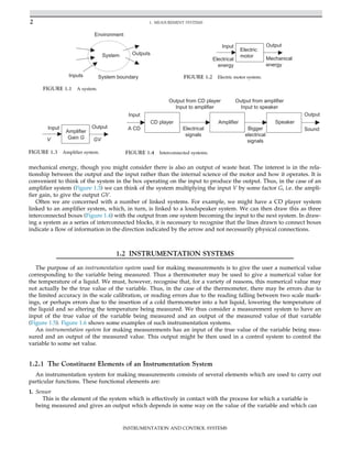
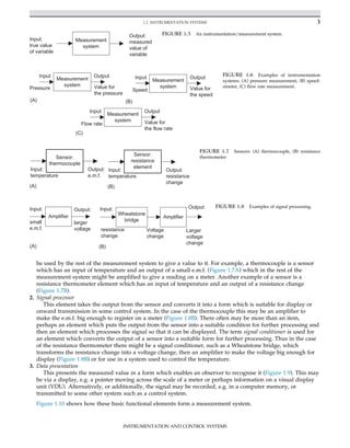
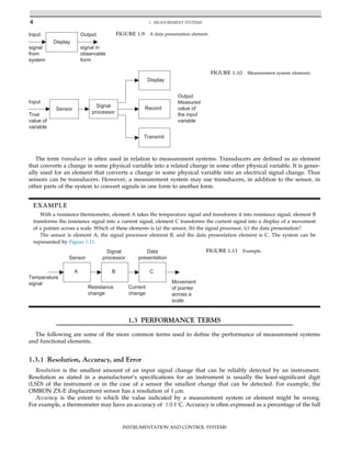
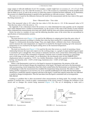
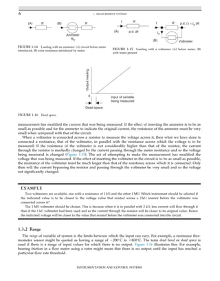
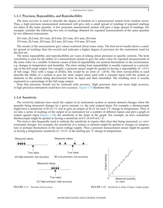
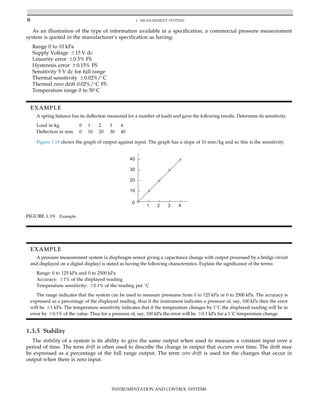
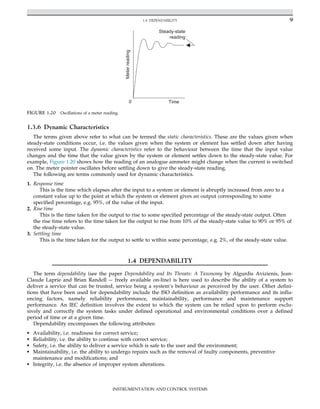
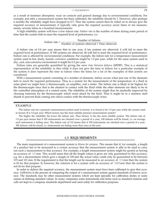
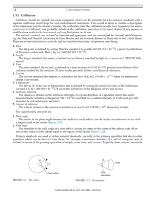
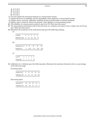
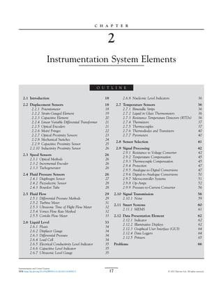
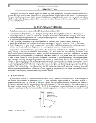
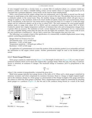
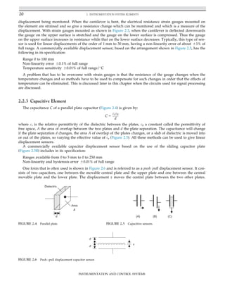
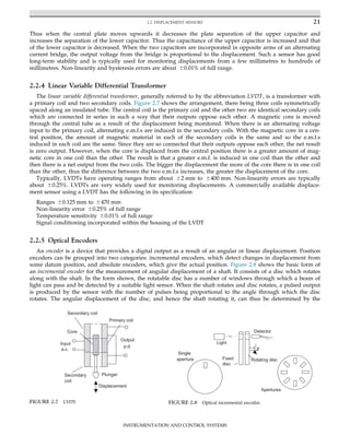
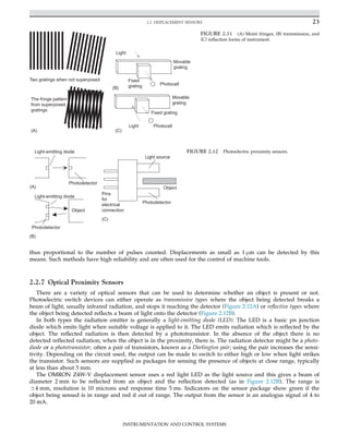
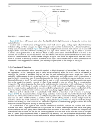
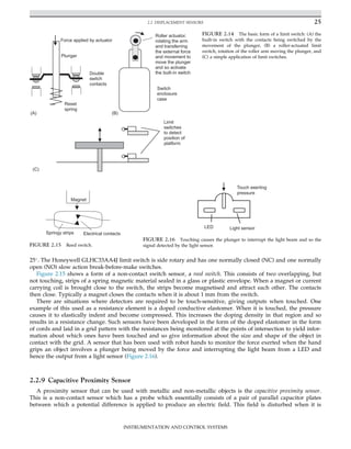
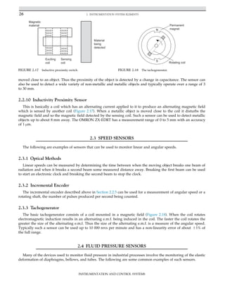
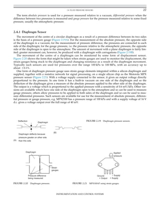
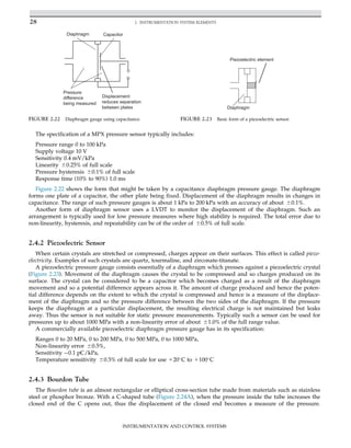
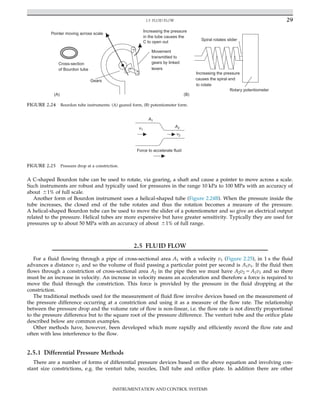
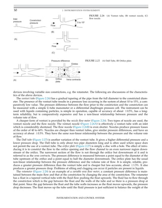
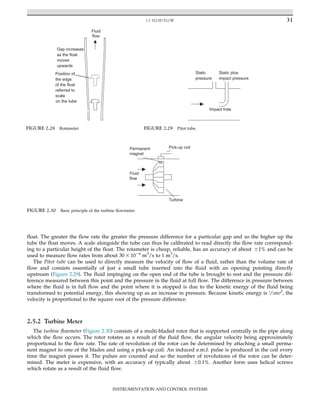
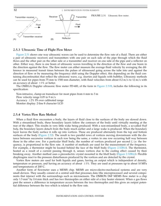
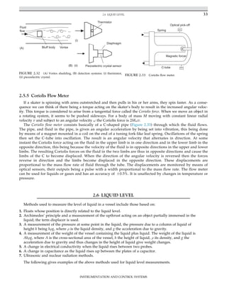
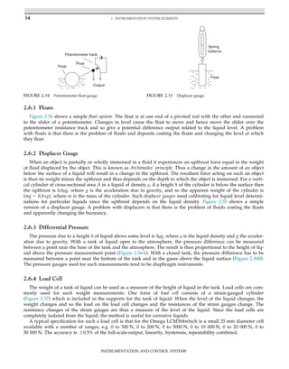
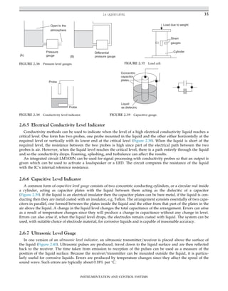
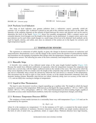
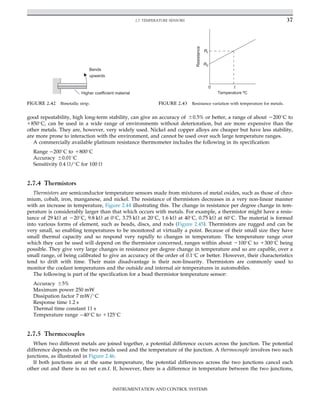
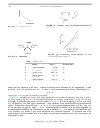
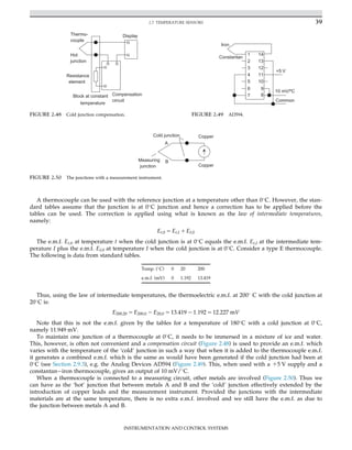
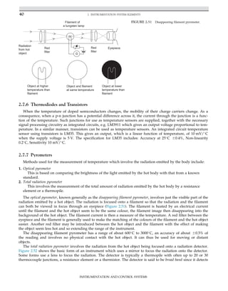


![his
JAMES + LEWIS.
mark.
MALCOM F. SMITH,
1st Lieutenant and Adjutant 6th U. S. Heavy Artillery, (colored.)
J. H. ODLIN,
Captain and A. A. G.
West's Buildings Hospital,
Baltimore, Md., May 24, 1864.
until most all the men were shot down. I was wounded and knocked
down with the but of a musket and left for dead, after being robbed,
and they cut the buttons off my jacket. I saw two women shot by
the river bank and their bodies thrown into the river after the place
was taken. I saw Frank Meek, company B, 6th United States heavy
artillery, (colored,) shot after he had surrendered.
Sworn to and subscribed before me this 30th day of April, 1864, at
Fort Pickering, Memphis, Tennessee.
A true copy.
[This evidence was received after the regular edition was printed.]
P. S. Since the report of the committee was prepared for the press,
the following letter from the surgeon in charge of the returned
prisoners was received by the chairman of the committee:
Dear Sir: I have the honor to enclose the photograph of John
Breinig, with the desired information written upon it. I am very sorry
your committee could not have seen these cases when first received.
No one, from these pictures, can form a true estimate of their](https://image.slidesharecdn.com/13423126-250603030250-0c549fa0/85/Instrumentation-And-Control-Systems-3rd-Edition-William-Bolton-73-320.jpg)