Downloaded 28 times


![XI
Chapter 1
Introduction
1.1 General Introduction
Evolutionary Algorithm (EA) is the study of computational system which use ideas and get
inspirations from natural evolution. It’s a generic population based meta-heuristic
optimization algorithm. EA falls into category of bio-inspired computing. It uses selection,
crossover, mutation mechanisms borrowed from natural evolution. And survival of the fittest
principle lies in the heart of EA [1] [2]. Evolution Algorithms are often viewed as function
optimizers, although the range of problems to which EAs are applies quite broad. One of the
many advantages of EAs is they don’t require very broad domain knowledge. Although
domain knowledge can be introduced in EAs.
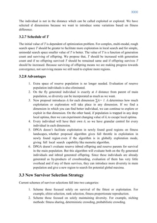
Fitness curve by generations for EA is asymptotic in nature. Fitness improvement in earlier
generations of EA is rapid and decreasingly increasing. And after certain generations,
improvement in best fitness throughout generations is negligible. That’s when we call
population has converged. It’s expected that population will converge to good enough
solution. But sometimes population converges to local optima which is not accepted result.
This phenomenon is called premature optimization.
Figure 1.1(a): Change in best fitness (best solution) with number of generations
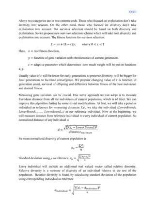
EAs performs better than random search because search because of its exploitative behavior.
It uses random walk, but also tries exploit good solutions. It also outperforms local greedy](https://image.slidesharecdn.com/evolutionaryalgorithmthesis-140604211101-phpapp02/85/Adaptive-Selection-in-Evolutionary-Algorithm-thesis-11-320.jpg)
![XII
search. Local greedy searches are exploitative in nature, often trapped into local maxima. But
EA has random walk and maintaining required level of diversity it’s less likely to be trapped
into local maxima. Problem tailored searches outperform EA only for the problem in which
the search is tailored and uses deep domain knowledge of that problem. Such deep domain
knowledge isn’t readily available and incorporating to problem tailored search is difficult.
Figure (1.1b): Comparison between Random Search, EA and Problem Tailored Search[4]
1.2 Thesis Objective
This thesis mainly focuses into maintaining diversity of single population algorithms. It is
frequently observed that populations lose diversity too early and their individuals are trapped
into local optima. For lack of diversity trapped individuals can’t escape basin of local
minima. This phenomenon is called Premature Convergence. Objective of this thesis paper is
to investigate better schemes which can maintain diversity of a population and also give
control on diversity. The quest is searching for an adaptive diversity maintaining scheme.
Thesis is done in three focused areas:
1. Modifying Dual Population Genetic Algorithm (DPGA) so that it can properly
manage diversity.
2. Seeking a survivor selection technique which is adaptive and gives more control
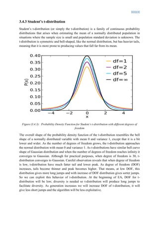
on diversity at any time of algorithm.
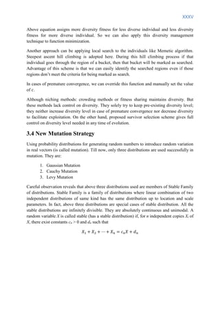
3. Examining probability distributions other than already used distributions which
can give appropriate amount of jumps in any stage of evolution.](https://image.slidesharecdn.com/evolutionaryalgorithmthesis-140604211101-phpapp02/85/Adaptive-Selection-in-Evolutionary-Algorithm-thesis-12-320.jpg)
![XVII
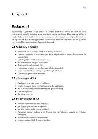
2.6 Major Branches of EA
EAs are divided into four major branches.
2.6.1 Genetic Algorithm
Genetic Algorithm (GA) was first formulated by John Holland. Holland’s original GA is
called standard Genetic Algorithm which uses two parents, produces two offspring. It
simulates Darwinian evolution. Search operators are only applied to genotypic representation;
hence it’s called Genotypic Algorithm. It emphasizes the role of crossover and mutation as a
background operator. GA uses binary string as representation of individuals extensively.
2.6.2 Evolutionary Programming
Evolutionary Programming (EP) was first proposed by David Fogel [2]. It is closer to
Lamarckian evolution. It doesn’t use any kind of crossover. Only mutation is used both for
exploitation and exploration. Individuals are represented by two parts: object variables and
mutation step size . are essentially real valued vectors i.e. phenotypes. So they are called
Phenotypic Algorithm.
2.6.3 Evolutionary Strategies
Evolutionary Strategies (ES) was first proposed by Ingred Rechenberg. Individuals are
represented by real valued vectors. Good optimizer of real valued functions. Like EP, they
are also Phenotypic Algorithm. Mutation plays the main role, crossover is also used. It has
special self-adapting step size of mutation. ES has some basic notation:
1. (p,c) The p parents 'produce' c children using mutation. Each of the c children is then
assigned a fitness value, depending on its quality considering the problem-specific
environment. The best (the fittest) p children become next generations parents. This
means the c children are sorted by their fitness value and the first p individuals are
selected to be next generations parents (c must be greater or equal p).
2. (p+c) The p parents 'produce' c children using mutation. Each of the c children is then
assigned a fitness value, depending on its quality considering the problem-specific
environment. The best (the fittest) p individuals of both: parents and children become
next generations parents. This means the c children together with the p parents are
sorted by their fitness value and the first p individuals are selected to be next
generations parents.
3. (p/r,c) The p parents 'produce' c children using mutation and recombination. Each of
the c children is then assigned a fitness value, depending on its quality considering the
problem-specific environment. The best (the fittest) p children become next
generations parents. This means the c children are sorted by their fitness value and the
first p individuals are selected to be next generation parents (c must be greater or
equal p).
4. (p+c) The p parents 'produce' c children using mutation and recombination. Each of
the c children is then assigned a fitness value, depending on its quality considering the
problem-specific environment. The best (the fittest) p individuals of both: parents and](https://image.slidesharecdn.com/evolutionaryalgorithmthesis-140604211101-phpapp02/85/Adaptive-Selection-in-Evolutionary-Algorithm-thesis-17-320.jpg)
![XIX
2.6.5 Memetic algorithm
Although Memetic algorithms don’t fall into EA category, they incorporate other searching
techniques to EAs. The combination of Evolutionary Algorithms with Local Search
Operators that work within the EA loop has been termed “Memetic Algorithms” (MA). Quite
often, MA are also referred to in the literature as Baldwinian Evolutionary algorithms (EA),
Lamarckian EAs, cultural algorithms or genetic local search. After generating individuals
local search is performed on them. The frequency and intensity of individual learning directly
define the degree of evolution (exploration) against individual learning (exploitation) in the
MA search, for a given fixed limited computational budget. Clearly, a more intense
individual learning provides greater chance of convergence to the local optima but limits the
amount of evolution that may be expended without incurring excessive computational
resources. Therefore, care should be taken when setting these two parameters to balance the
computational budget available in achieving maximum search performance. When only a
portion of the population individuals undergo learning, the issues on which subset of
individuals to improve need to be considered to maximize the utility of MA search.
2.7 Existing Works
2.7.1 Dynamic Parameter Control
A variety of previous works have proposed methods of dynamically adjusting the parameters
of GA or other evolutionary algorithms. These methods include deterministic parameter
control, adaptive parameter control, and self-adaptive parameter control. The simplest
technique is the deterministic parameter control, which adjusts parameters according to a
predetermined policy. Since it controls the parameters deterministically, it cannot adapt to the
changes that occur during the execution of an algorithm.
Adaptive parameter control exploits feedback from the evolution of a population to control
the parameters. A notable example is the 1:5 adaptive Gaussian mutation widely used in the
evolution strategy algorithms. According to this method, the mutation step size is increased if
more than 20% of the mutations are successful and reduced otherwise. However, this method
cannot be applied to algorithms adopting other than the real number representation. Finally,
self-adaptive parameter control encodes the parameters into chromosomes and let them
evolve with other genes. Although elegant, its applicability and effectiveness in a broad range
of problems have not yet been shown
2.7.2 Maintaining Diversity and Multi-population Genetic Algorithms
Multi population GAs (MPGAs) do so by evolving multiple subpopulations which are
spatially separated [6]. Island-model GA (IMGA), which is a typical example of MPGA,
evolves two or more subpopulations and uses periodic migration for the exchange of
information between the subpopulations. The number and size of the populations of IMGA](https://image.slidesharecdn.com/evolutionaryalgorithmthesis-140604211101-phpapp02/85/Adaptive-Selection-in-Evolutionary-Algorithm-thesis-19-320.jpg)
![XXIII
4. Fitness Proportionate Reproduction: Same as roulette wheel selection scheme.
Individuals are directly transferred to next generation based on their proportionate
fitness value. Individuals of lower fitness still have some chances to survive, so that
some genes that are latent can survive through generations even so they haven’t been
able to generate good individuals.
5. Niching Methods: Niching methods strive to maintain niches [9] [10]. That means it
ensures individuals of one niche don’t have to compete with individuals of other
niches. The advantage is pre-existing diversity is maintained. But also makes
convergence harder as selection pressure is lower. Niching methods are divided into
two categories:
i) Fitness Sharing: In nature, individuals of same species compete with each other
for fixed resources [13]. Like nature, in fitness sharing, individuals in same region
share fixed fitness values assigned to that region. Fitness is a shared resource of
the population. Population is first divided into niches. Region is defined by
sharing radius . Sharing Radius defines the niche size. This scheme is
very sensitive to the value of assigned fitness per region and sharing radius.
Population does not converge as a whole, but convergence takes place within the
niches. Sharing can be done at genotypic or phenotypic level: 1. Genotypic level:
Hamming distance and 2. Phenotypic Level: Euclidean distance. Sharing radius: if
too small, practically no effect on the process; if too large, several peaks will
’melt’ individual peaks into one.
ii) Crowding: Similar individuals in natural population, often of the same species,
compete against each other for limited resources. Dissimilar individuals tend to
occupy different niches, they typically don’t compete. Crowding uses individuals
newly entering in a population to replace similar individuals. Random sample of
CF (Crowding Factor) individuals is taken from the population. Larger crowding
factor indicates less tolerance for the similar solutions, smaller values indicate
similar solutions are more welcomed. New members of particular species replace
older members of that species, not replacing members of other species. Crowding
doesn’t increase the diversity of population; rather it strives to maintain the pre-
existing diversity. It’s not directly influenced by fitness value. Crowding is
divided into:
(1) Deterministic Crowding: New individual will always replace the most similar
individual if it has better fitness value.
(2) Probabilistic Crowding: Primarily a distance based niching method. Main
difference is the use of a probabilistic rather than deterministic acceptance
function. No longer do stronger individuals win over weaker individuals, they
win proportionally according to their fitness, and thus we get restorative
pressure. Two core ideas of probabilistic crowding are to hold tournament
between similar individuals and to let tournaments be probabilistic.
6. Deterministic Sampling: Average fitness of the population is calculated. Fitness
associated to each individual is divided by the average fitness, but only the integer
part of this operation is stored. If the value is equal or higher than one, the individual](https://image.slidesharecdn.com/evolutionaryalgorithmthesis-140604211101-phpapp02/85/Adaptive-Selection-in-Evolutionary-Algorithm-thesis-23-320.jpg)

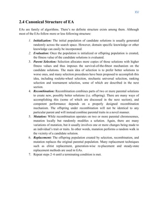
![XXV
Chapter 3
Algorithm Proposal
3.1 Dual Population Genetic Algorithm
Dual Population Genetic Algorithm (DPGA) is a genetic algorithm which uses two
populations instead of one to avoid premature convergence with two different evolutionary
objectives [11] [12] [13]. The main population plays the role of that of an ordinary genetic
algorithm. It evolves to find a good solution of high fitness value. The additional population
is called reserve population is employed as reservoir for additional chromosomes which are
rather different from chromosomes of main population. Two different fitness functions are
used. Main population uses actual fitness function (like normal GA) and reserve population
uses a fitness function which gives better fitness to the chromosomes more different from
chromosomes of main population. Multi Population Genetic Algorithms use migration of
chromosomes from one population to another population to exchange information. DPGA
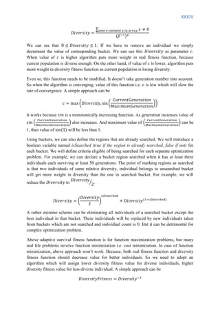
doesn’t use migration instead it uses another noble approach called crossbreeding.
Crossbreeding is performed by taking one parent from main population and another parent
from reserve population, making crossover between them. Newly born offspring are called
crossbred offspring. Crossbred offspring then evaluated for both main population and reserve
population for survival. DPGA also employs inbreeding, which takes two parents from the
same population and makes offspring by crossover. These inbred offspring compete for
survival in their respective parent population.
Figure (3.1a): Offspring Generation of DPGA
Mutation plays minimal role in DPGA and diversity is mainly provided by reserve population
through crossbreeding. Crossbreeding plays the role of maintaining diversity in DPGA. The
amount of diversity needed in any step of DPGA is specified by a self-adaptive parameter δ
(0< δ <1). δ defines the distance of parents from main population and parents from reserve](https://image.slidesharecdn.com/evolutionaryalgorithmthesis-140604211101-phpapp02/85/Adaptive-Selection-in-Evolutionary-Algorithm-thesis-25-320.jpg)
![XLV
References
[1] D.E. Goldberg, Genetic Algorithms in Search, Optimization, and Machine Learning.
Addison-Wesley, Reading, MA, 1989.
[2] L.J. Fogel, A.J. Owens, and M.J. Walsh, Artificial Intelligence through simulated
evolution, New York, John Wiley & Sons, 1966.
[3] E. Eiben, R. Hinterding, and Z. Michalewicz, “Parameter control in evolutionary
algorithms,” IEEE Trans. Evol. Comput., vol. 3, no. 2, pp. 124–141, Jul. 1999.
[4] D. H. Wolpert and W. G. Macready, “No free lunch theorems for optimization”, IEEE
Transactions on Evolutionary Computation, vol. 1, no. 1, pp. 67–82, 1997.
[5] D. E. Goldberg and J. Richardson, “Genetic algorithms with sharing for multimodal
function optimization,” in Proc. 2nd Int. Conf. Genetic Algorithms (ICGA), 1987, pp. 41–49.
[6] T. Jumonji, G. Chakraborty, H. Mabuchi, and M. Matsuhara, “A novel distributed genetic
algorithm implementation with variable number of islands,” in Proc. IEEE Congr. Evolut.
Comput., 2007, pp. 4698–4705.
[7] Y. Yoshida and N. Adachi, “A diploid genetic algorithm for preserving population
diversity-pseudo-Meiosis GA,” in Proc. 3rd Parallel Problem Solving Nature (PPSN), 1994,
pp. 36–45.
[8] M. Kominami and T. Hamagami, “A new genetic algorithm with diploid chromosomes by
using probability decoding for nonstationary function optimization,” in Proc. IEEE Int. Conf.
Syst., Man, Cybern., 2007, pp. 1268–1273.
[9] S. W. Mahfoud, “Crowding and preselection revisited,” in Proc. 2nd Parallel Problem
Solving Nature (PPSN), 1992, pp. 27–37.
[10] S. W. Mahfoud, “Niching methods for genetic algorithms,” Ph.D. dis-sertation, Dept.
General Eng., Univ. Illinois, Urbana-Champaign, 1995.
[11] T. Park and K. R. Ryu, “A dual population genetic algorithm with evolving diversity,” in
Proc. IEEE Congr. Evol. Comput. , 2007, pp. 3516–3522.
[12] T. Park and K. R. Ryu, “Adjusting population distance for dual-population genetic
algorithm,” in Proc. Aust. Joint Conf. Artif. Intell., 2007, pp. 171–180.
[13] T. Park and K. R. Ryu, “A Dual-Population Genetic Algorithm for Adaptive Diversity
Control” in Proc. Aust. Joint Conf. Artif. Intell., 2009, pp. 191–210.
[13] R. McKay, “Fitness sharing in genetic programming,” in Proc. of the Genetic and
Evolutionary Computation Conference, Las Vegas, Nevada, 2000, pp. 435–442.](https://image.slidesharecdn.com/evolutionaryalgorithmthesis-140604211101-phpapp02/85/Adaptive-Selection-in-Evolutionary-Algorithm-thesis-45-320.jpg)
![XLVI
[14] R. K. Ursem, “Diversity guided Evolutionary algorithm,” in Proc. of Parallel Problem
Solving from Nature (PPSN) VII, vol. 2439, J. J. Merelo, P. Adamidis, H. P. Schwefel, Eds.
Granada, Spain, 2002, pp. 462–471.
[15] T. Bäck and H.-P. Schwefel, “An overview of evolutionary algorithms for parameter
optimization,” Evol. Comput., vol. 1, pp. 1–23, 1993.
[16] K. Chellapilla, “Combining mutation operators in evolutionary programming,” IEEE
Trans. Evol. Comput., vol. 2, pp. 91–96, Sept. 1998.
[17] R. Mantegna, “Fast, accurate algorithm for numerical simulation of Lévy stable
stochastic process,” Phys. Rev. E, vol. 49, no. 5, pp. 4677–4683, 1994.
[18] X. Yao, G. Lin, and Y. Liu, “An analysis of evolutionary algorithms based on
neighborhood and step size,” in Proc. 6th Int. Conf. Evolutionary Programming, 1997, pp.
297–307
[19] D. Thierens, “Adaptive mutation rate control schemes in genetic algorithms,” in Proc.
Congr. Evol. Comput. , vol. 1. 2002, pp. 980–985.
[20] G. Rudolph, “On takeover times in spatially structured populations: Array and ring,” in
Proc. 2nd Asia-Pacific Conf. Genetic Algorithms Applicat., 2000, pp. 144–151.
[21] X. Yao, Y. Liu, and G. Lin, “Evolutionary programming made faster,” IEEE Trans.
Evol. Comput., vol. 3, no. 2, pp. 82–102, Jul. 1999.](https://image.slidesharecdn.com/evolutionaryalgorithmthesis-140604211101-phpapp02/85/Adaptive-Selection-in-Evolutionary-Algorithm-thesis-46-320.jpg)

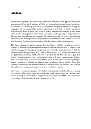
This document summarizes an adaptive selection scheme proposed by Muhammad Riyad Parvez for his thesis. It contains 5 chapters: 1. Introduction outlines the objectives of developing a selection scheme to balance exploitation and exploration in evolutionary algorithms. 2. Background provides context on evolutionary algorithms and discusses existing work on parameter control, maintaining diversity, and survivor selection. 3. Proposed Algorithms introduces a modified dual population genetic algorithm, a new adaptive survivor selection strategy, and new mutation strategies based on probability distributions like Laplace and Student's t-distribution. 4. Experimental Study evaluates the modified dual population genetic algorithm and adaptive survivor selection strategy on benchmark problems and compares results with other methods. The adaptive selection strategy showed better