Download as PDF, PPTX

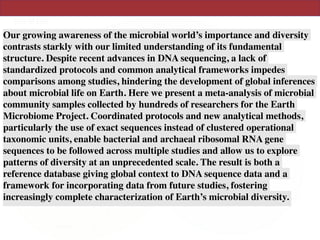
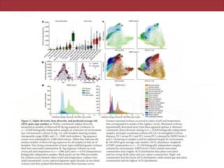
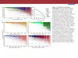
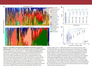
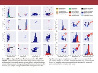

The document describes a meta-analysis of microbial community samples collected by the Earth Microbiome Project (EMP) that used coordinated protocols and analytical methods to explore patterns of diversity at an unprecedented scale. By tracking individual bacterial and archaeal ribosomal RNA gene sequences across multiple studies, the analysis resulted in both a reference database providing global context to DNA sequence data and an analytical framework for incorporating future study data to further characterize Earth's microbial diversity. The meta-analysis found that standardized environmental descriptors and new analytical methods, particularly using exact sequences instead of clustered operational taxonomic units, enabled comparisons across studies and exploration of large-scale ecological patterns.


