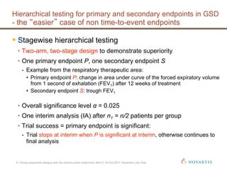
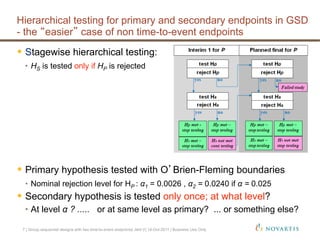
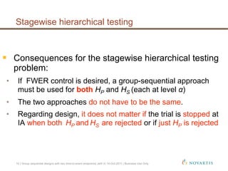
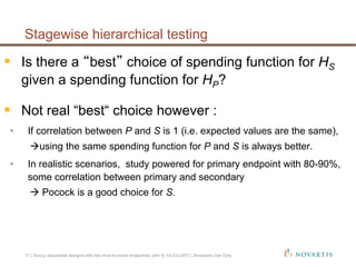
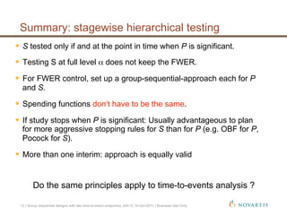
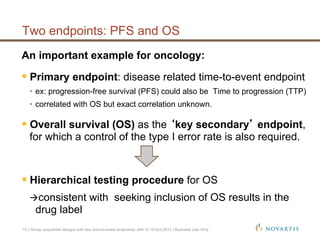
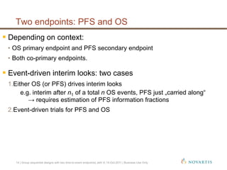
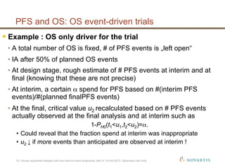
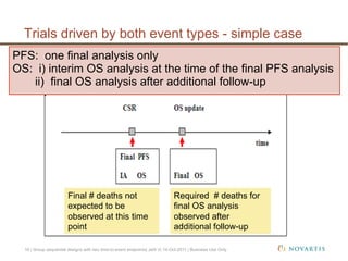
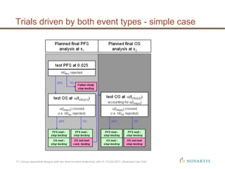
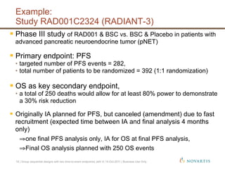
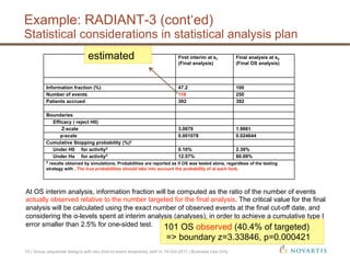
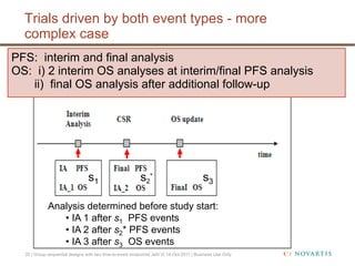
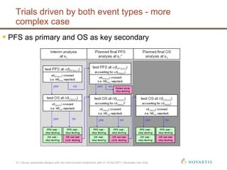
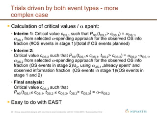
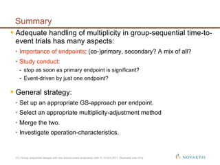
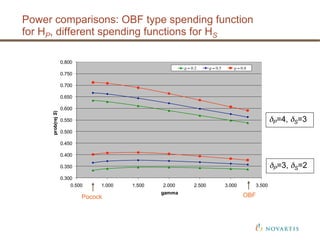
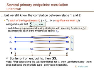
This document discusses approaches for handling multiple time-to-event endpoints in group sequential clinical trial designs. It provides examples of hierarchical testing procedures where the secondary endpoint is only evaluated if the primary endpoint is significant. It also discusses approaches where trials are driven by both primary and secondary event types, with interim analyses planned for each endpoint. Maintaining control of the overall type I error rate across multiple analyses and endpoints is an important consideration.

1. Group sequential designs with two
time-to-event endpoints
Valentine Jehl, Novartis Pharma AG, Switzerland
Paris, 14-Oct-2011

2. Objective
 Give a few examples on how designs with two time-to-
event can be implemented
 Provide the rational for chosen strategies
2 | Presentation Title | Presenter Name | Date | Subject | Business Use Only

3. 3 | Group sequential designs with two time-to-event endpoints| Jehl V| 14-Oct-2011 | Business Use Only
Motivations
 In oncology, time-to-event type variables are the most
commonly used endpoints for phase III trials
 Ex. Progression free survival, Overall survival
 Objective of the phase III = proof of efficacy as soon as
possible
 Condideration of group sequential design with interim looks
 Consideration of surrogate endpoints, if applicable
 Multiple tests performed
 Multiplicity has to be taken into account

4. Definition
 Primary endpoint
• should be the clinical measures that best characterize the
efficacy of the treatment, and used to judge the overall success
of the study.
• should be clinically meaningful, and, ideally, fully characterize
the treatment effect
 Secondary endpoint
• may provide additional characterization of the treatment effect.
• if positive might be mentionned in the label
4 | Group sequential designs with two time-to-event endpoints| Jehl V| 14-Oct-2011 | Business Use Only

5. Handling multiplicity
 How to deal with more than one endpoints in a group
sequential design (GSD)?
• Hierachical procedure
• Different spending functions
• Simultaneous testing
5 | Group sequential designs with two time-to-event endpoints| Jehl V| 14-Oct-2011 | Business Use Only

6.  Stagewise hierarchical testing
• Two-arm, two-stage design to demonstrate superiority
• One primary endpoint P, one secondary endpoint S
- Example from the respiratory therapeutic area:
• Primary endpoint P: change in area under curve of the forced expiratory volume
from 1 second of exhalation (FEV1) after 12 weeks of treatment
• Secondary endpoint S: trough FEV1
• Overall significance level α = 0.025
• One interim analysis (IA) after n1 = n/2 patients per group
• Trial success = primary endpoint is significant:
- Trial stops at interim when P is significant at interim, otherwise continues to
final analysis
Hierarchical testing for primary and secondary endpoints in GSD
- the easier case of non time-to-event endpoints
6 | Group sequential designs with two time-to-event endpoints| Jehl V| 14-Oct-2011 | Business Use Only

7. Hierarchical testing for primary and secondary endpoints in GSD
- the easier case of non time-to-event endpoints
 Stagewise hierarchical testing:
• HS is tested only if HP is rejected
 Primary hypothesis tested with O Brien-Fleming boundaries
• Nominal rejection level for HP : α1 = 0.0026 , α2 = 0.0240 if α = 0.025
 Secondary hypothesis is tested only once; at what level?
• At level α ? ..... or at same level as primary? ... or something else?
7 | Group sequential designs with two time-to-event endpoints| Jehl V| 14-Oct-2011 | Business Use Only

8.  Naive idea:
Since S is tested only once and only when P was
significant, S can be tested at full level α
This is not true!
 Naive strategy leads to type I error rate inflation
• (Hung, Wang and O‘Neill (2007))
Inflation of type I error rate for HS
8 | Group sequential designs with two time-to-event endpoints| Jehl V| 14-Oct-2011 | Business Use Only

9.  Maximum type I error for conditional testing HS at level α is
• For n1/n = 0.5 and α = 0.025, maximum type I error is 0.041.
 Significance level for HS must be adjusted to keep a given
significance level αS for the secondary variable
 For conditional testing HS at levels α*1 = α*2 = 0.0147 > α/2,
the maximum type I error attained is αS = 0.025
• α*1 = α*2 are the „Pocock -boundaries
( )2 1 1 11 , ; /z z n nα α− −− Φ
Actually, it can be shown that …
9 | Group sequential designs with two time-to-event endpoints| Jehl V| 14-Oct-2011 | Business Use Only

10.  Consequences for the stagewise hierarchical testing
problem:
• If FWER control is desired, a group-sequential approach
must be used for both HP and HS (each at level α)
• The two approaches do not have to be the same.
• Regarding design, it does not matter if the trial is stopped at
IA when both HP and HS are rejected or if just HP is rejected
Stagewise hierarchical testing
10 | Group sequential designs with two time-to-event endpoints| Jehl V| 14-Oct-2011 | Business Use Only

11.  Is there a best choice of spending function for HS
given a spending function for HP?
 Not real “best“ choice however :
• If correlation between P and S is 1 (i.e. expected values are the same),
using the same spending function for P and S is always better.
• In realistic scenarios, study powered for primary endpoint with 80-90%,
some correlation between primary and secondary
 Pocock is a good choice for S.
Stagewise hierarchical testing
11 | Group sequential designs with two time-to-event endpoints| Jehl V| 14-Oct-2011 | Business Use Only

12.  S tested only if and at the point in time when P is significant.
 Testing S at full level α does not keep the FWER.
 For FWER control, set up a group-sequential-approach each for P
and S.
 Spending functions don‘t have to be the same.
 If study stops when P is significant: Usually advantageous to plan
for more aggressive stopping rules for S than for P (e.g. OBF for P,
Pocock for S).
 More than one interim: approach is equally valid
Do the same principles apply to time-to-events analysis ?
Summary: stagewise hierarchical testing
12 | Group sequential designs with two time-to-event endpoints| Jehl V| 14-Oct-2011 | Business Use Only

13. An important example for oncology:
 Primary endpoint: disease related time-to-event endpoint
• ex: progression-free survival (PFS) could also be Time to progression (TTP)
• correlated with OS but exact correlation unknown.
 Overall survival (OS) as the key secondary endpoint,
for which a control of the type I error rate is also required.
 Hierarchical testing procedure for OS
consistent with seeking inclusion of OS results in the
drug label
Two endpoints: PFS and OS
13 | Group sequential designs with two time-to-event endpoints| Jehl V| 14-Oct-2011 | Business Use Only

14.  Depending on context:
• OS primary endpoint and PFS secondary endpoint
• Both co-primary endpoints.
 Event-driven interim looks: two cases
1. Either OS (or PFS) drives interim looks
e.g. interim after n1 of a total n OS events, PFS just „carried along“
→ requires estimation of PFS information fractions
2. Event-driven trials for PFS and OS
Two endpoints: PFS and OS
14 | Group sequential designs with two time-to-event endpoints| Jehl V| 14-Oct-2011 | Business Use Only

15.  Example : OS only driver for the trial
• A total number of OS is fixed, # of PFS events is „left open“
• IA after 50% of planned OS events
• At design stage, rough estimate of # PFS events at interim and at
final (knowing that these are not precise)
• At interim, a certain α spend for PFS based on #(interim PFS
events)/#(planned finalPFS events)
• At the final, critical value u2 recalculated based on # PFS events
actually observed at the final analysis and at interim such as
1-PH0(t1<u1,t2<u2)=α.
• Could reveal that the fraction spend at interim was inappropriate
• u2 ↓ if more events than anticipated are observed at interim !
PFS and OS: OS event-driven trials
15 | Group sequential designs with two time-to-event endpoints| Jehl V| 14-Oct-2011 | Business Use Only

16. PFS: one final analysis only
OS: i) interim OS analysis at the time of the final PFS analysis
ii) final OS analysis after additional follow-up
Final # deaths not
expected to be
observed at this time
point
Required # deaths for
final OS analysis
observed after
additional follow-up
Trials driven by both event types - simple case
16 | Group sequential designs with two time-to-event endpoints| Jehl V| 14-Oct-2011 | Business Use Only

17. Trials driven by both event types - simple case
17 | Group sequential designs with two time-to-event endpoints| Jehl V| 14-Oct-2011 | Business Use Only

18. Example:
Study RAD001C2324 (RADIANT-3)
 Phase III study of RAD001 & BSC vs. BSC & Placebo in patients with
advanced pancreatic neuroendocrine tumor (pNET)
 Primary endpoint: PFS
• targeted number of PFS events = 282,
• total number of patients to be randomized = 392 (1:1 randomization)
 OS as key secondary endpoint,
• a total of 250 deaths would allow for at least 80% power to demonstrate
a 30% risk reduction
 Originally IA planned for PFS, but canceled (amendment) due to fast
recruitment (expected time between IA and final analysis 4 months
only)
⇒ one final PFS analysis only, IA for OS at final PFS analysis,
⇒ Final OS analysis planned with 250 OS events
18 | Group sequential designs with two time-to-event endpoints| Jehl V| 14-Oct-2011 | Business Use Only

19. First interim at s1
(Final analysis)
Final analysis at s2
(Final OS analysis)
Information fraction (%) 47.2 100
Number of events 118 250
Patients accrued 392 392
Boundaries
Efficacy ( reject H0)
Z-scale 3.0679 1.9661
p-scale 0.001078 0.024644
Cumulative Stopping probability (%)2
Under H0 for activity2 0.10% 2.39%
Under Ha for activity2 12.57% 80.09%
2 results obtained by simulations. Probabilities are reported as if OS was tested alone, regardless of the testing
strategy with . The true probabilities should take into account the probability of at each look.
At OS interim analysis, information fraction will be computed as the ratio of the number of events
actually observed relative to the number targeted for the final analysis. The critical value for the final
analysis will be calculated using the exact number of observed events at the final cut-off date, and
considering the α-levels spent at interim analysis (analyses), in order to achieve a cumulative type I
error smaller than 2.5% for one-sided test.
Example: RADIANT-3 (cont‘ed)
Statistical considerations in statistical analysis plan
estimated
101 OS observed (40.4% of targeted)
=> boundary z=3.33846, p=0.000421
19 | Group sequential designs with two time-to-event endpoints| Jehl V| 14-Oct-2011 | Business Use Only

20. PFS: interim and final analysis
OS: i) 2 interim OS analyses at interim/final PFS analysis
ii) final OS analysis after additional follow-up
s1 s2
* s3
Analysis determined before study start:
• IA 1 after s1 PFS events
• IA 2 after s2* PFS events
• IA 3 after s3 OS events
Trials driven by both event types - more
complex case
20 | Group sequential designs with two time-to-event endpoints| Jehl V| 14-Oct-2011 | Business Use Only

21.  PFS as primary and OS as key secondary
Trials driven by both event types - more
complex case
21 | Group sequential designs with two time-to-event endpoints| Jehl V| 14-Oct-2011 | Business Use Only

22.  Calculation of critical values / α spent:
• Interim 1: Critical value cOS,1 such that PH0 (tOS,1> cOS,1) = αOS,1,
αOS,1 from selected α-spending approach for the observed OS info
fraction (#OS events in stage 1)/(total # OS events planned)
• Interim 2:
Critical value cOS,2 such that PH0 (tOS,1≤ cOS,1, tOS,2> cOS,2) = αOS,2 -αOS,1,
αOS,2 from selected α-spending approach for the observed OS info
fraction (OS events in stage 2)/s3, using αOS,1 „already spent“ and
observed information fraction (OS events in stage 1)/(OS events in
stage 1 and 2)
• Final analysis:
Critical value cOS,3 such that
PH0 (tOS,1≤ cOS,1, tOS,2 ≤ cOS,2, tOS,3> cOS,3) = α-αOS,2
 Easy to do with EAST
Trials driven by both event types - more
complex case
22 | Group sequential designs with two time-to-event endpoints| Jehl V| 14-Oct-2011 | Business Use Only

23.  Adequate handling of multiplicity in group-sequential time-to-
event trials has many aspects:
• Importance of endpoints: (co-)primary, secondary? A mix of all?
• Study conduct:
- stop as soon as primary endpoint is significant?
- Event-driven by just one endpoint?
 General strategy:
• Set up an appropriate GS-approach per endpoint.
• Select an appropriate multiplicity-adjustment method
• Merge the two.
• Investigate operation-characteristics.
Summary
23 | Group sequential designs with two time-to-event endpoints| Jehl V| 14-Oct-2011 | Business Use Only

24. Thank you
24 | Group sequential designs with two time-to-event endpoints| Jehl V| 14-Oct-2011 | Business Use Only
For providing this material
• Ekkehard Glimm
• Norbert Hollaender

25. Back up slides
25 | Presentation Title | Presenter Name | Date | Subject | Business Use Only

26. 0.300
0.350
0.400
0.450
0.500
0.550
0.600
0.650
0.700
0.750
0.800
0.500 1.000 1.500 2.000 2.500 3.000 3.500
prob(rejS)
gamma
ρ = 0.2 ρ = 0.5 ρ = 0.8
OBFPocock
δP=4, δS=3
δP=3, δS=2
Power comparisons: OBF type spending function
for HP, different spending functions for HS

27. ... but we still know the correlation between stage 1 and 2
 To each of the hypotheses Hj, j = 1,…,h, a significance level αj is
assigned such that
• and define group sequential testing strategies with spending functions ai(y)
separately for each of the hypotheses at level αj .
1
h
jj
α α=
=∑
t 0 1 2 3
H1
H2
Hh
α1
α2
αh
 Bonferroni on endpoints, then GS.
Note: First calculating the GS boundaries for α, then „bonferronizing“ them
does not keep the multiple type I error rate in general.
Several primary endpoints: correlation
unknown