Lecture 1 basic concepts2009

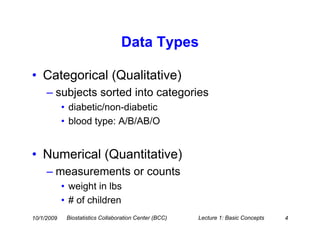
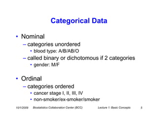
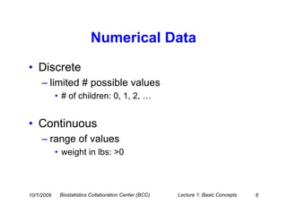
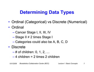
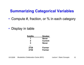
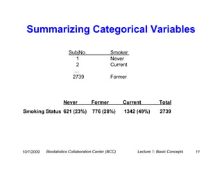
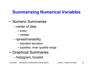
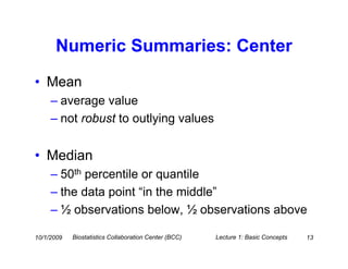
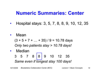
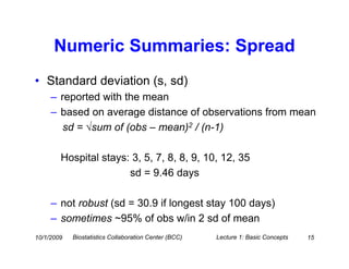
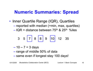
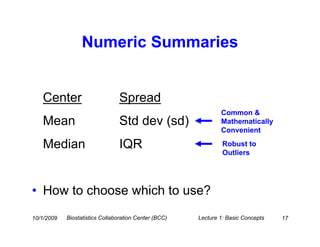
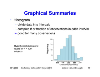
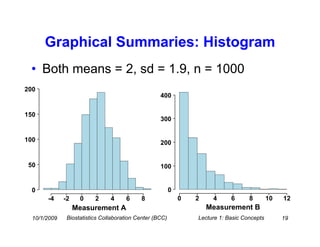
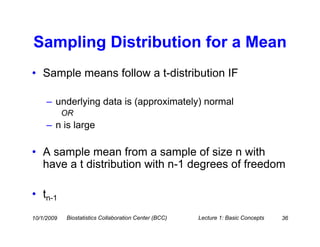
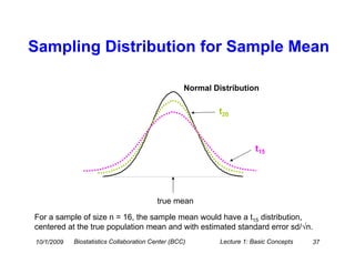
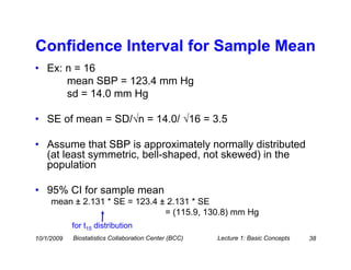
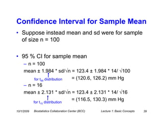
Basic Biostatistics in Medical Research

Lecture 1: Basic Concepts

Leah J. Welty, PhD
Biostatistics Collaboration Center (BCC)
Department of Preventive Medicine
NU Feinberg School of Medicine

Objectives
• Assist participants in interpreting statistics
published in medical literature

• Highlight different statistical methodology
for investigators conducting own research

• Facilitate communication between medical
investigators and biostatisticians
10/1/2009 Biostatistics Collaboration Center (BCC) Lecture 1: Basic Concepts 2

Lecture 1: Basic Concepts

Data Types
Summary Statistics
One Sample Inference

Data Types

• Categorical (Qualitative)
– subjects sorted into categories
• diabetic/non-diabetic
• blood type: A/B/AB/O

• Numerical (Quantitative)
– measurements or counts
• weight in lbs
• # of children

Categorical Data

• Nominal
– categories unordered
• blood type: A/B/AB/O
– called binary or dichotomous if 2 categories
• gender: M/F

• Ordinal
– categories ordered
• cancer stage I, II, III, IV
• non-smoker/ex-smoker/smoker

Numerical Data
• Discrete
– limited # possible values
• # of children: 0, 1, 2, …

• Continuous
– range of values
• weight in lbs: >0


Determining Data Types
• Ordinal (Categorical) vs Discrete (Numerical)
• Ordinal
– Cancer Stage I, II, III, IV
– Stage II ≠ 2 times Stage I
– Categories could also be A, B, C, D
• Discrete
– # of children: 0, 1, 2, …
– 4 children = 2 times 2 children

Determining Data Types

• Type of data determines which types of
analyses are appropriate

• Continuous vs. Categorical


Describing Data
• General summary
– condense information to manageable form
– numerically
• ‘center’ of data values
• spread of data; variability
– graphically/visually

• What analyses are / are not appropriate


Summarizing Categorical Variables
• Compute #, fraction, or % in each category

• Display in table

SubjNo Smoker
1 Never
2 Current
3 Never
…
2738 Former
2739 Former


Summarizing Categorical Variables

SubjNo Smoker
1 Never
2 Current
…
2739 Former

Never Former Current Total
Smoking Status 621 (23%) 776 (28%) 1342 (49%) 2739


Summarizing Numerical Variables

• Numeric Summaries
– center of data
• mean
• median
– spread/variability
• standard deviation
• quartiles; inner quartile range
• Graphical Summaries
– histogram, boxplot

Numeric Summaries: Center
• Mean
– average value
– not robust to outlying values

• Median
– 50th percentile or quantile
– the data point “in the middle”
– ½ observations below, ½ observations above


Numeric Summaries: Center
• Hospital stays: 3, 5, 7, 8, 8, 9, 10, 12, 35

• Mean
(3 + 5 + 7 + … + 35) / 9 = 10.78 days
Only two patients stay > 10.78 days!
• Median
3 5 7 8 8 9 10 12 35
Same even if longest stay 100 days!

Numeric Summaries: Spread
• Standard deviation (s, sd)
– reported with the mean
– based on average distance of observations from mean
sd = √sum of (obs – mean)2 / (n-1)

Hospital stays: 3, 5, 7, 8, 8, 9, 10, 12, 35
sd = 9.46 days

– not robust (sd = 30.9 if longest stay 100 days)
– sometimes ~95% of obs w/in 2 sd of mean

Numeric Summaries: Spread
• Inner Quartile Range (IQR), Quartiles
– reported with median (+min, max, quartiles)
– IQR = distance between 75th & 25th %iles

3 5 7 8 8 9 10 12 35

– 10 – 7 = 3 days
– range of middle 50% of data
– same even if longest stay 100 days!

Numeric Summaries

Center Spread
Common &
Mean Std dev (sd) Mathematically
Convenient

Median IQR Robust to
Outliers

• How to choose which to use?

Graphical Summaries
• Histogram
– divide data into intervals
– compute # or fraction of observations in each interval
– good for many observations
20

15
Frequency
Hypothetical cholesterol
levels for n = 100 10
subjects
5

0
160 180 200 220 240
Cholesterol (mg/100mL)

Graphical Summaries: Histogram
• Both means = 2, sd = 1.9, n = 1000
200
400

150
300

100 200

50 100

0 0
-4 -2 0 2 4 6 8 0 2 4 6 8 10 12
Measurement A Measurement B

Graphical Summaries: Histogram
• Both means = 2, sd = 1.9, n = 1000
200
400

median = 2
150
IQR = 2.8 300

100 200

50
median = 1.4
100
IQR = 2.1

0 0
-4 -2 0 2 4 6 8 0 2 4 6 8 10 12
Measurement A Measurement B

Graphical Summaries: Boxplots
• Graphical extension of median, IQR

• Useful for comparing two variables

• Help identify ‘outliers’


Maximum
240
Cholesterol Levels (mg/100mL)

220
Q3 (75th %ile)

200 IQR Median

Q1 (25th %ile)
180

160 Minimum


Maximum
10 “outliers”
all greater than
Q3 + 1.5 * IQR

5 largest obs less
than Q3 + 1.5 * IQR
IQR

0 Minimum

-5
Var 1
Measurement A Var 2
Measurement B

Data Type & Data Summaries
• Type determines appropriate summary

• Characteristics of data determined in
summary determine appropriate analyses
– more than just mean, sd
– e.g. should not use t for strongly skewed data
– median (IQR) appropriate if skewed, outliers


Statistical Inference
• Estimation of quantity of interest
– estimate itself
– quantify how good an estimate it is

• Hypothesis testing
– Is there evidence to suggest that the estimate
is different from another value?

• Today: proportion, mean, median

• Take results obtained in a (random) sample as
best estimate of what is true for the population

• Estimate may differ from the population value by
chance, but it should be close

• How good is the estimate?

• If we took more samples, and got even more
estimates, how would they vary?

• Ex: proportion of persons in a population who
have health insurance, sample size n = 978

Sample 1 797/978 = 0.81

We conclude that the estimated % of people with health
insurance is 81%.

How variable is our estimate?


Sampling Variability
• Need to know the sampling distribution for
the quantity of interest

• One option: take lots of samples, and
make a histogram

Sample 2 782/978 = 0.80
Sample 3 812/978 = 0.83

Sampling Variability
• Not practical to keep repeating a study!

• Statistical theory

– the sampling distributions for means and proportions
often look “normal”, bell-shaped

– from a single sample, can calculate the standard error
(variability) of our estimated mean or proportion


Standard Error
• Standard error (SE) measures the variability of
your sample statistic (e.g. a mean or proportion)

• small SE means estimate more precise

• SE is not the same as SD!

• SD measures the variability of the sample data;
SE measures the variability of the statistic

Standard Error vs Standard Deviation
• Averages less variable than the individual observations

• Averages over larger n less variable than over smaller n

• Ex: heights

– most people from 5’0” – 6’2”
– average height for sample of 100 people ~ between 5’5” – 5’7”

• SE ≤ SD!


Inference for Sample Proportions
• Formula for SE of sample proportion

prop ⋅ (1 − prop )
n

• For health insurance example
– n = 978, prop = 0.81
– SE = √(0.81) * (0.19)/978 = 0.01
– The standard error of the sample proportion is 0.01.


Sampling Distribution of Sample
Proportion
• Sample proportions are normally distributed if (prop) * (1-prop) * n > 10
• if ≤ 10, then need to use exact binomial (not covered here)

~ 95% of sample
proportions within ~2
SEs of true proportion

true proportion – 1.96 SE true proportion true proportion + 1.96 SE


Confidence Interval for Sample
Proportion
• 95% Confidence Interval for Sample Proportion

(sample prop – 1.96 * SE, sample prop + 1.96 * SE)

• Interpretation: For about 95/100 samples, this interval will contain
the true population proportion

• 95% CI for % population with insurance (n = 978, prop = 0.81)

Check: (0.81) * (1-0.81) * 978 = 150.5 > 10

95% CI: (0.81 – 1.96 * 0.01, 0.81 + 1.96 * 0.01) =
(0.79, 0.83)

• For greater confidence (e.g. 99%CI), wider interval


Standard Error for Sample Mean
• Standard error is the standard deviation of the sample,
divided by the square root of the sample size

SE = SD/√n

• Ex: n = 16
mean SBP = 123.4 mm Hg
sd = 14.0 mm Hg

• SE of mean = SD/√n = 14.0/ √16 = 3.5


Sampling Distribution for a Mean
• Sample means follow a t-distribution IF

– underlying data is (approximately) normal
OR
– n is large

• A sample mean from a sample of size n with
have a t distribution with n-1 degrees of freedom

• tn-1

Sampling Distribution for Sample Mean

Normal Distribution

t20

t15

true mean

For a sample of size n = 16, the sample mean would have a t15 distribution,
centered at the true population mean and with estimated standard error sd/√n.

Confidence Interval for Sample Mean
• Ex: n = 16
mean SBP = 123.4 mm Hg
sd = 14.0 mm Hg

• SE of mean = SD/√n = 14.0/ √16 = 3.5

• Assume that SBP is approximately normally distributed
(at least symmetric, bell-shaped, not skewed) in the
population

• 95% CI for sample mean
mean ± 2.131 * SE = 123.4 ± 2.131 * SE
= (115.9, 130.8) mm Hg
for t15 distribution

• Suppose instead mean and sd were for sample
of size n = 100

• 95 % CI for sample mean
– n = 100
mean ± 1.984 * sd/√n = 123.4 ± 1.984 * 14/ √100
for t99 distribution = (120.6, 126.2) mm Hg
– n = 16
mean ± 2.131 * sd/√n = 123.4 ± 2.131 * 14/ √16
for t distribution
= (116.5, 130.3) mm Hg
15


• Suppose instead mean and s were for sample of
size n = 100

• 95 % CI for sample mean
– n = 100
mean ± 1.984 * sd/√n = 123.4 ± 1.984 * 14/ √100
= (120.6, 126.2) mm Hg
– n = 16
mean ± 2.131 * sd/√n = 123.4 ± 2.131 * 14/ √16
= (116.5, 130.3) mm Hg


Confidence Interval for a Sample
Mean
• Confession: it’s never incorrect to use a t-
distribution (as long as underlying
population normal or n large)

BUT

as n gets large the t-distribution and
normal distribution become
indistinguishable

Hypothesis Testing

• Confidence intervals tell you
– best estimate
– variability of best estimate

• Hypothesis testing
– Is there really a difference between my
observed value and another value?

Hypothesis Testing
• From our sample of n = 978, we estimated
that 81% of the people in our population
had health insurance.
• From previous census records, you know
that 10 years ago, 78.5% of your
population had health insurance.
• Has the percent of people with insurance
really changed?


Hypothesis Testing
• Suppose the true percent with health insurance is 78.5%
– Called the null hypothesis, or H0

• What is the probability of observing, for a sample of n = 978, a result
as or more extreme than 81%, given the true percent is 78.5%?
– Called the p-value, computed using normal distribution for sample
proportions (and t-distribution for sample means)

• If probability is small, conclude that supposition might not be right.
– Reject the null hypothesis in favor of the alternative hypothesis, Ha
(opposite of the null hypothesis, related to what you think may be true)

• If the probability is not small, conclude do not have evidence to
reject the null hypothesis
– Not the same as ‘accepting’ the null hypothesis, or showing that the null
hypothesis is true


Hypothesis Testing
H0: True proportion is 78.5% opposites
Ha: True proportion is not 78.5%

P-value = Prob(sample prop >
0.81 or sample prop < 0.76
given true prop = 0.785) = 0.012

0.76 0.81
Supposed true
proportion = 0.785

Hypothesis Testing
• It is not very likely (p = 0.012) to observe our data if the
true proportion is 78.5%.

• We conclude that we have sufficient evidence that the
proportion insured is no longer 78.5%.

• “Two-sided” test: observations as extreme as 0.81
> 0.81 or < 0.76

• “One-sided” test: observations larger than 0.81
– Has the percent of people with insurance really increased?
– Ha: True proportion greater than 78.5%
– p-value = 0.006 (only area above 0.81)
– Only ok if previous research suggests that the prop is larger


Hypothesis Testing
• Similar for sample means, except that p-values
are computed using t-distribution, if appropriate

• n = 16 with SBP = 123.4, sd = 14.0 mm Hg

• Previous research suggests that population may
have lifestyle habits protective for high BP

• Do we have evidence to suggest that our
population has SBP lower than 125 mm Hg (pre-
hypertensive)?

Hypothesis Testing
H0: True mean is 125 mm Hg almost opposites
Ha: True mean is less than 125 mm Hg

• Using t15 distribution, we find a one-sided
p-value of 0.32

• This too large to reject the null hypothesis
in favor of the alternative.
– Usually need p < 0.05 to “reject null” in favor
of alternative

Misinterpretations of the p-value
• A p-value of 0.32 (or > 0.05) DOES NOT mean that we
“accept the null”, or that there is a 32% chance that the
null is true

– we haven’t shown that the SBP of this group is equal to 125
– true value may be 124.5 or 125.1 mmHg

• Can only “reject the null in favor of the alternative” or “fail
to reject the null”

• If you “fail to reject” that doesn’t mean the alternative
isn’t true. You may not have had a large enough n!


Distribution-Free Alternatives
• Recall for the normal distribution to be useful for sample
proportions, we need n * prop * (1-prop) > 10

– If not, use exact binomial methods (not covered here)

• For the t-distribution to be useful for sample means, we
need the underlying population to be normal or n large

– What if this isn’t the case?
• data are skewed or n is small
• e.g. length of hospital stay
– Use nonparametric methods
• look at ranks, not mean
• the median is a nonparametric estimate


Nonparametric Methods
• nonparametric methods are methods that don’t require
assuming a particular distribution

• a.k.a distribution-free or rank methods

• nonparametric tests well suited to hypothesis testing

• not as useful for point estimates or CIs

• espeically useful when data are ranks or scores
– Apgar scores
– Vision (20/20, 20/40, etc.)


Nonparametric Methods for Sample
Median
• Alternative to using sample mean & t-distribution
• Instead do inference for median value
– CI for median uses ranks
• n = 16, ~ 95% CI for median
(4th largest value, 13th largest value)
• n = 25, ~ 95% CI for median
(8th largest value, 18th largest value)
• necessary ranks depend on n and confidence level
Stat packages or tables

– Hypothesis test for median: Sign Test


Sign Test for the Median
• Hypothesis about median, not mean

• Assuming hypothesized value of median is
correct, expect to observe about half
sample below median and half above.

• Compute probability for (as or more
extreme) proportion above median

Sign Test Example
• Average daily energy intake over 10 ID Energy Intake
days for 11 healthy subjects 1 5260
2 5470
3 5640
• Are these subjects getting the
4 6180
recommended level of 7725 kJ?
5 6390
6 6515
• Data aren’t strongly skewed, but we 7 6805
don’t know if underlying population 8 7515
is normal, and n is small 9 7515
10 8230
• Use sign test to see if median level 11 8770
for population might be 7725 kJ


Sign Test
• Expect about half values above 7725 kJ

• Only 2/11 subjects values above the 7725 kJ

• If the probability of selecting a subject whose
value is above 7725 kJ is ½, what’s the
probability of obtaining a sample of 11 subjects
in which 2 or fewer are above 7725 kJ?

• p-value = 0.1019 (from stat software)

Parametric vs. Nonparametric
• Nonparametric always okay
• Nonparametric more conservative than
parametric
– e.g. 95% CIs for medians sometimes twice as
wide as those for the mean
• If your data satisfy the requirements, or n
is fairly large, probably best to use
parametric procedures


Useful References
• Intuitive Biostatistics, Harvey Motulsky, Oxford
University Press, 1995
– Highly readable, minimally technical

• Practical Statistics for Medical Research,
Douglas G. Altman, Chapman & Hall, 1991
– Readable, not too technical

• Fundamentals of Biostatistics, Bernard Rosner,
Duxbury, 2000
– Useful reference, somewhat technical


Next Time

Two group comparisons


Contact BCC
• Please go to our web site at:
http://www.medschool.northwestern.edu
/depts/bcc/index.htm

• Fill out our online request form for further
collaboration!


Lecture 1 basic concepts2009

More Related Content

Viewers also liked

Similar to Lecture 1 basic concepts2009

Recently uploaded

Lecture 1 basic concepts2009