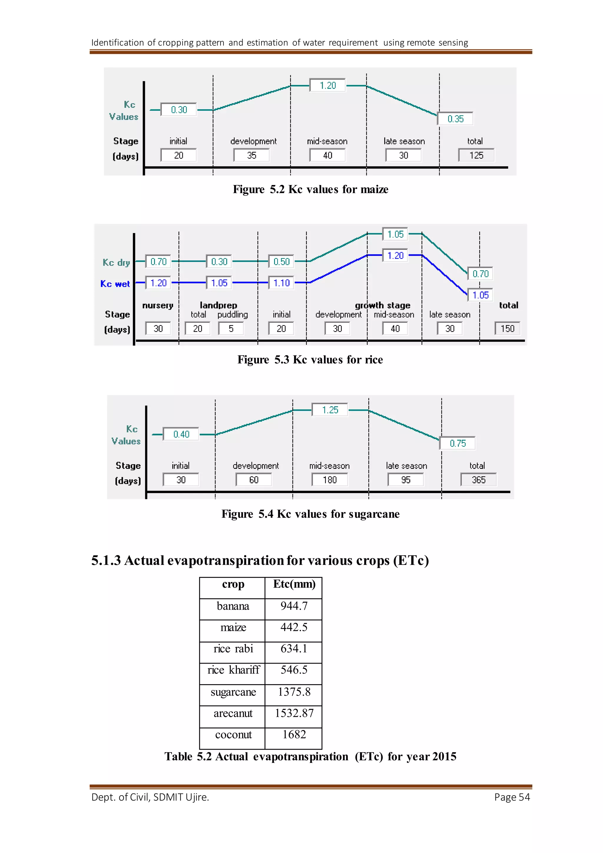
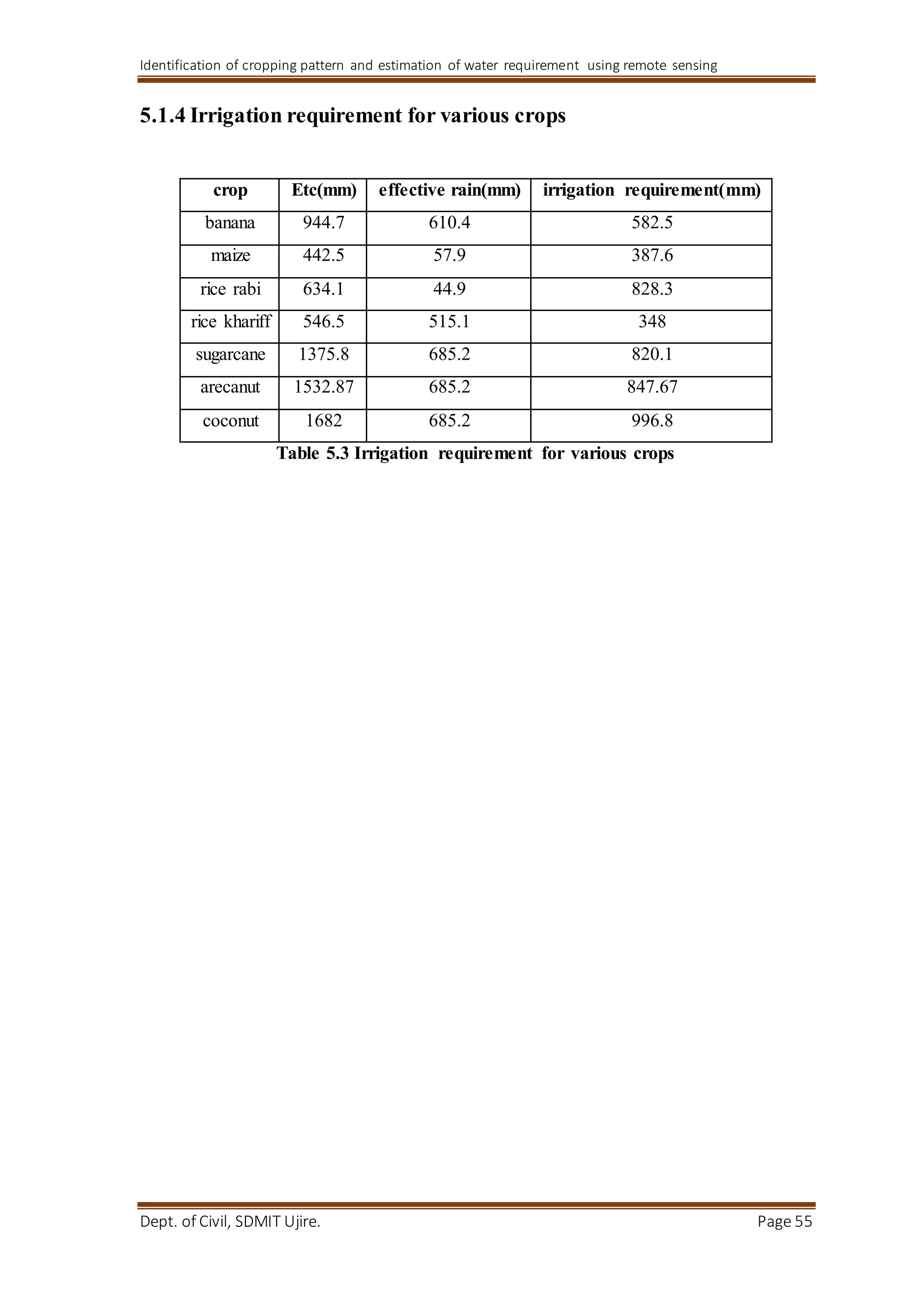
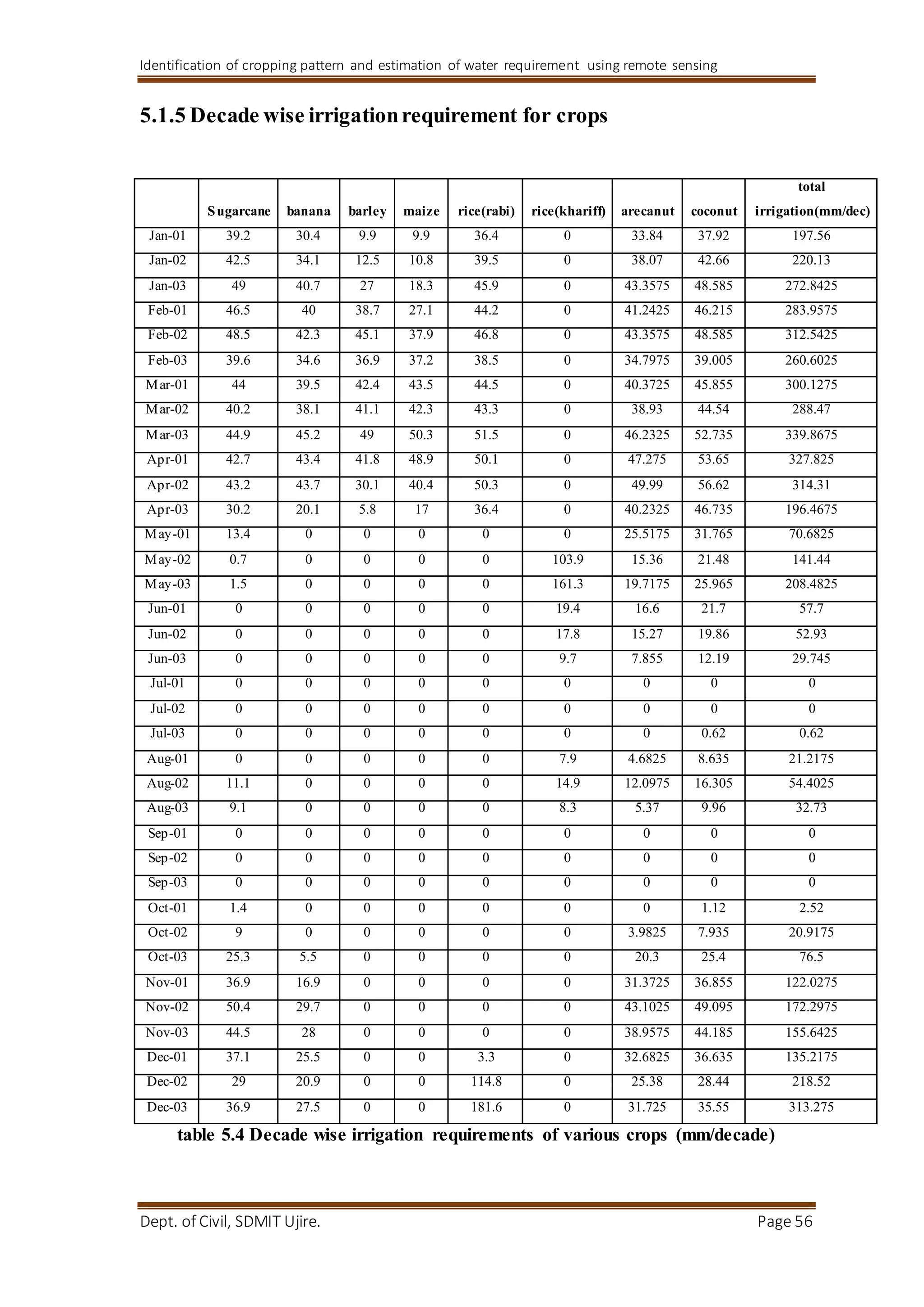
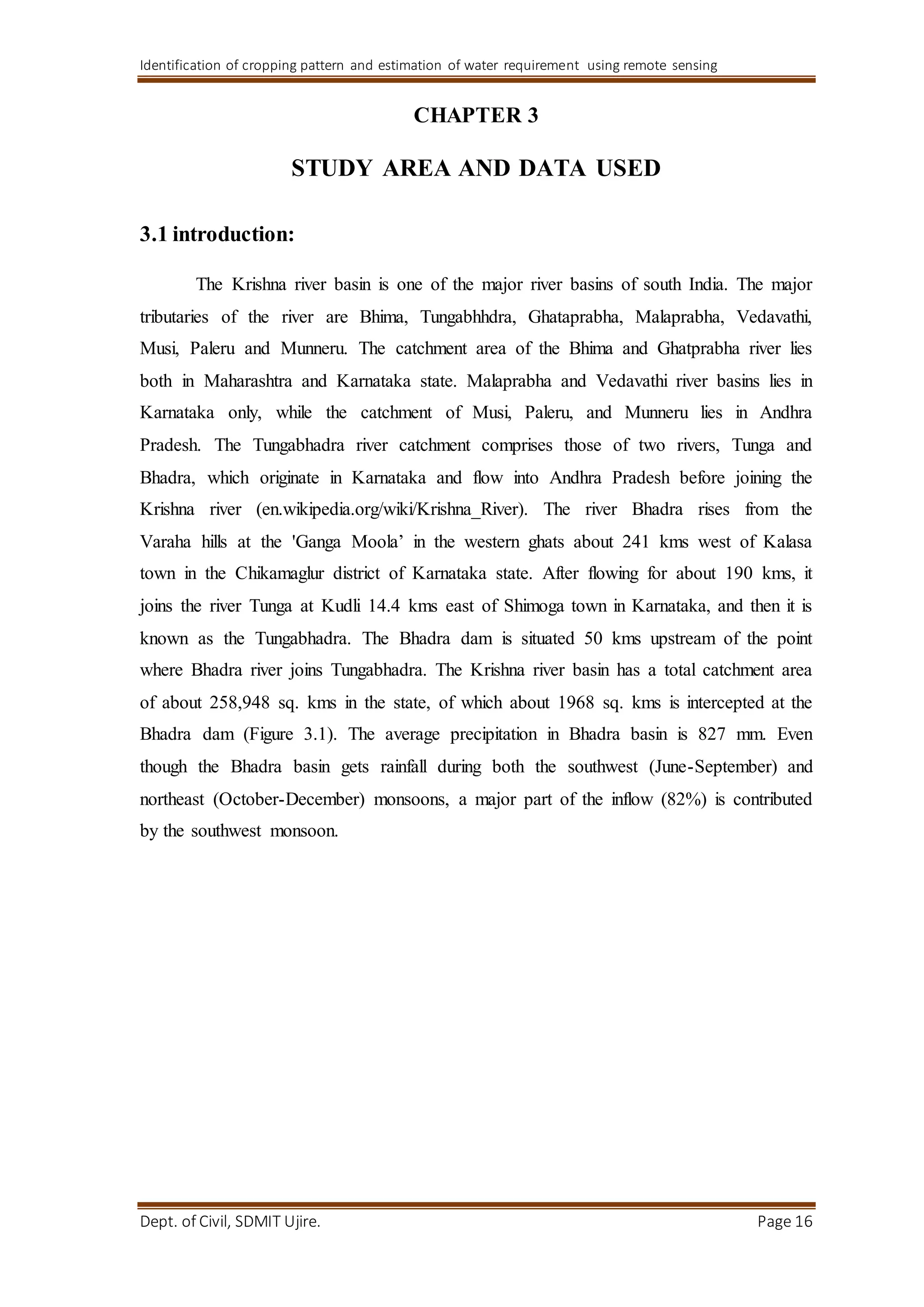
What are the advantages and disadvantages of membrane structures.pptx
estimation of irrigation requirement using remote sensing
1. Identification of cropping pattern and estimation of water requirement using remote sensing
Dept. of Civil, SDMIT Ujire. Page 1
CHAPTER 1
INTRODUCTION
The water requirement has been increasing more and more especially in
agriculture. The agricultural sector makes use of 75% of the water withdrawn from river,
lakes and aquifers (Wallace, 2000). In recent years irrigated land has developed rapidly.
Water increasingly often becomes a limiting factor for food production especially in dry
climates. In dry climates water sources are very limited since the amount of rain-fall is
very low. As the total size of the hot dry areas in the world is about 45-50 million square
kilometres (Dregne, 1976) which means one third of the total land area of the world.
In dry climate the availability of water for irrigation of crops is limited, which
restricts the possibility for cultivation of crops. For that reason a lot of research has been
done to develop methods to protect water and using less amount of fresh water as far as
possible without effects on crops yield, and to increase water use efficiency in irrigation
without any negative effects on crop yields.
Thus irrigation scheduling is one of the best methods which can help us to realize these
aims. The irrigation scheduling consists of two parts;
The first part is to determine the water requirement (the right amount of water). This
can be done by different methods, like determine the amount of evapotranspiration
of the crop.
The second part is to estimate the right time to supply the water to plants there are
several methods that can be used to decide when to irrigate crops.
1.1. Background
Irrigation scheduling involves determining both the timing of irrigation and the
quantity of water to apply. It is an essential daily management practice for a farm
manager growing irrigated crops. Proper timing of irrigation can be done by monitoring
the soil water content or monitoring the crop in the field. Plant stress responses provide
the most direct measure of identifying the plant demand for water. However, it should be
noted that while plant stress indicators provide a direct measure of when water is
required, they do not provide a direct volumetric measure of the volume of water required
to be applied.
The crop water requirement is defined as amount of water required to compensate
the evapotranspiration loss from the cropped field (Allen et al., 1998). Many researchers
2. Identification of cropping pattern and estimation of water requirement using remote sensing
Dept. of Civil, SDMIT Ujire. Page 2
describe it as the total water needed for evapotranspiration. Therefore, the water
requirement can be decided by determining the actual evapotranspiration.
The crop water requirement can be related to the amount of water used by a
reference crop. The reference crop typically is grass or alfalfa that is well irrigated and
covers 100 % of the ground. The reference evapotranspiration ETo includes the water
evaporated from the soil surface and the water transpired by the plants.
The daily reference evapotranspiration ETo can also be calculated from daily climate data
like temperature, wind speed, sunshine and relative humidity. There are several methods
used to calculate or measure ETo.
The most common methods are Penman method, Pan Evaporation and Blaney-
Criddle method. The climate data can be obtained from a weather station.
The actual evapotranspiration can be calculated by multiplying the calculated reference
evapotranspiration with a crop coefficient factor, Kc. The crop coefficient factor values
represent the crop type and its characteristics and the development of the crop.
The successful irrigation scheduling requires good understanding to the knowledge of soil
water holding capacity, crop water use, and crop sensitivity to moisture stress at different
growth stages. This requires consideration about the effective rainfall, and availability of
irrigation water (Waskom, 1994).
1.2. Water Balance
Water balance was used to calculate the theoretical irrigation requirements for
comparison with actual irrigation water applied. The demand for water by the crop must
be met by the water in the soil, via the root system. The actual rate of water uptake by the
crop from the soil in relation to its maximum evapotranspiration is determined by whether
the available water in the soil is adequate or whether the crop will suffer from stress
inducing water deficit. In order to determine Etc, the level of the available soil water must
be considered. Eta equals maximum evapo-transpiration when available soil water to the
crop is adequate, the irrigation water requirement is considered nil. However, Etc is less
than maximum evapotranspiration when available soil water is limited. The magnitude of
ETa can be quantified for periods between irrigation and heavy rain .
3. Identification of cropping pattern and estimation of water requirement using remote sensing
Dept. of Civil, SDMIT Ujire. Page 3
1.3. Evapotranspiration Process
Combination of two separate processes whereby water is lost on the one hand
from the soil surface by evaporation and on the other hand from the crop by transpiration
is referred to as evapotranspiration (ETo).
1.3.1 Evaporation
Evaporation is the process whereby liquid water is converted to water vapour
(vaporization) and removed from the evaporating surface (vapour removal). Water
evaporates from a variety of surfaces, such as lakes, rivers, pavements, soils and wet
vegetation.Where the evaporating surface is the soil surface, the degree of shading of the
crop canopy and the amount of water available at the evaporating surface are other factors
that affect the evaporation process. Frequent rains, irrigation and water transported
upwards in a soil from a shallow water table wet the soil surface. Where the soil is able to
supply water fast enough to satisfy the evaporation demand, the evaporation from the soil
is determined only by the meteorological conditions.
1.3.2. Transpiration
Transpiration consists of the vaporization of liquid water contained in plant tissues
and the vapour removal to the atmosphere. Crops predominately lose their water through
stomata. These are small openings on the plant leaf through which gases and water
vapour pass (Figure 1.1). The water, together with some nutrients, is taken up by the roots
and transported through the plant.
The vaporization occurs within the leaf, namely in the intercellular spaces, and
the vapour exchange with the atmosphere is controlled by the stomatal aperture. Nearly
all water taken up is lost by transpiration and only a tiny fraction is used within the plant.
4. Identification of cropping pattern and estimation of water requirement using remote sensing
Dept. of Civil, SDMIT Ujire. Page 4
Figure 1.1 Schematic representation of a stoma
Transpiration, like direct evaporation, depends on the energy supply, vapour
pressure gradient and wind. Hence, radiation, air temperature, air humidity and wind
terms should be considered when assessing transpiration. The soil water content and the
ability of the soil to conduct water to the roots also determine the transpiration rate, as do
waterlogging and soil water salinity. The transpiration rate is also influenced by crop
characteristics, environmental aspects and cultivation practices.
1.3.3. Evapotranspiration (ET)
Evaporation and transpiration occur simultaneously and there is no easy way of
distinguishing between the two processes. Apart from the water availability in the topsoil,
the evaporation from a cropped soil is mainly determined by the fraction of the solar
radiation reaching the soil surface. This fraction decreases over the growing period as the
crop develops and the crop canopy shades more and more of the ground area. When the
crop is small, water is predominately lost by soil evaporation, but once the crop is well
developed and completely covers the soil, transpiration becomes the main process. In
Figure 1.2 the partitioning of evapotranspiration into evaporation and transpiration is
plotted in correspondence to leaf area per unit surface of soil below it. At sowing nearly
100% of ET comes from evaporation, while at full crop cover more than 90% of ET
comes from transpiration.
5. Identification of cropping pattern and estimation of water requirement using remote sensing
Dept. of Civil, SDMIT Ujire. Page 5
Figure 1.2 schematic diagram of partitioning of evapotranspiration into
evaporation and transpiration over the growing period for an annual field crop.
1.3.4. Factors Affecting Evapotranspiration
Weather parameters, crop characteristics, management and environmental aspects
are factors affecting evaporation and transpiration. The related ET concepts presented in
Figure 1.3 are discussed in the section on evapotranspiration concepts.
Fig 1.3 Factors affecting evapotranspiration with reference to related ET concepts
6. Identification of cropping pattern and estimation of water requirement using remote sensing
Dept. of Civil, SDMIT Ujire. Page 6
1.3.5. Weatherparameters
The principal weather parameters affecting evapotranspiration are radiation, air
temperature, humidity and wind speed. Several procedures have been developed to assess
the evaporation rate from these parameters. The evaporation power of the atmosphere is
expressed by the reference crop evapotranspiration (ETo). The reference crop
evapotranspiration represents the evapotranspiration from a standardized vegetated
surface.
1.3.6. Cropfactors
The crop type, variety and development stage should be considered when
assessing the evapotranspiration from crops grown in large, well-managed fields.
Differences in resistance to transpiration, crop height, crop roughness, reflection, ground
cover and crop rooting characteristics result in different ET levels in different types of
crops under identical environmental conditions. Crop evapotranspiration under standard
conditions (ETc) refers to the evaporating demand from crops that are grown in large
fields under optimum soil water, excellent management and environmental conditions,
and achieve full production under the given climatic conditions.
1.4. Management and environmental conditions
Factors such as soil salinity, poor land fertility, limited application of fertilizers,
the presence of hard or impenetrable soil horizons, the absence of control of diseases and
pests and poor soil management may limit the crop development and reduce the
evapotranspiration. Other factors to be considered when assessing ET are ground cover,
plant density and the soil water content. The effect of soil water content on ET is
conditioned primarily by the magnitude of the water deficit and the type of soil. On the
other hand, too much water will result in waterlogging which might damage the root and
limit root water uptake by inhibiting respiration.
1.5. Evapotranspiration Concepts
Distinctions are made (Figure 1.4) between reference crop evapotranspiration
(ETo), crop evapotranspiration under standard conditions (ETc) and crop
evapotranspiration under nonstandard conditions (ETc adj). ETo is a climatic parameter
7. Identification of cropping pattern and estimation of water requirement using remote sensing
Dept. of Civil, SDMIT Ujire. Page 7
expressing the evaporation power of the atmosphere. ETc refers to the evapotranspiration
from excellently managed, large, wellwatered fields that achieve full production under the
given climatic conditions. Due to suboptimal crop management and environmental
constraints that affect crop growth and limit evapotranspiration, ETc under non-standard
conditions generally requires a correction.
Fig 1.4 Reference (ETo), crop evapotranspiration under standard (ETc) and non-
standard conditions (ETc adj)
1.5.1. Reference crop evapotranspiration (ETo)
The evapotranspiration rate from a reference surface, not short of water, is called
the reference crop evapotranspiration or reference evapotranspiration and is denoted as
ETo. The reference surface is a hypothetical grass reference crop with specific
characteristics. The use of other denominations such as potential ET is strongly
discouraged due to ambiguities in their definitions.
The concept of the reference evapotranspiration was introduced to study the
evaporative demand of the atmosphere independently of crop type, crop development and
management practices. As water is abundantly available at the reference evapotranspiring
surface, soil factors do not affect ET. Relating ET to a specific surface provides a
reference to which ET from other surfaces can be related. It obviates the need to define a
8. Identification of cropping pattern and estimation of water requirement using remote sensing
Dept. of Civil, SDMIT Ujire. Page 8
separate ET level for each crop and stage of growth. ETo values measured or calculated at
different locations or in different seasons are comparable as they refer to the ET from the
same reference surface.
The only factors affecting ETo are climatic parameters. Consequently, ETo is a
climatic parameter and can be computed from weather data. ETo expresses the
evaporating power of the atmosphere at a specific location and time of the year and does
not consider the crop characteristics and soil factors. The FAO Penman-Monteith method
is recommended as the sole method for determining ETo. The method has been selected
because it closely approximates grass ETo at the location evaluated, is physically based,
and explicitly incorporates both physiological and aerodynamic parameters.
TABLE 1.1 Average ETo for different agroclimatic regions in mm/day
Region Mean daily temperature(0c)
Cool
-10 oc
Moderate
20 oc
Warm
>30 oc
Tropics and subtropics
-humid and sub-humid
-arid and semi-arid
2-3
2-4
3-5
4-6
5-7
6-8
Temperature region
-humid and sub-humid
-arid and semi-arid
1-2
1-3
2-4
4-7
4-7
6-9
1.5.2. Crop evapotranspiration under standard conditions (ETc)
The crop evapotranspiration under standard conditions, denoted as ETc, is the
evapotranspiration from disease-free, well-fertilized crops, grown in large fields, under
optimum soil water conditions, and achieving full production under the given climatic
conditions.
The amount of water required to compensate the evapotranspiration loss from the
cropped field is defined as crop water requirement. Although the values for crop
evapotranspiration and crop water requirement are identical, crop water requirement
refers to the amount of water that needs to be supplied, while crop evapotranspiration
refers to the amount of water that is lost through evapotranspiration. The irrigation water
9. Identification of cropping pattern and estimation of water requirement using remote sensing
Dept. of Civil, SDMIT Ujire. Page 9
requirement basically represents the difference between the crop water requirement and
effective precipitation. The irrigation water requirement also includes additional water for
leaching of salts and to compensate for non-uniformity of water application.
Crop evapotranspiration can be calculated from climatic data and by integrating
directly the crop resistance, albedo and air resistance factors in the Penman-Monteith
approach. As there is still a considerable lack of information for different crops, the
Penman-Monteith method is used for the estimation of the standard reference crop to
determine its evapotranspiration rate, i.e., ETo. Experimentally determined ratios of
ETc/ETo, called crop coefficients (Kc), are used to relate ETc to ETo or ETc = Kc.ETo.
1.5.3. Crop evapotranspiration under non-standard conditions (ETc adj)
The crop evapotranspiration under non-standard conditions (ETc adj) is the
evapotranspiration from crops grown under management and environmental conditions
that differ from the standard conditions. When cultivating crops in fields, the real crop
evapotranspiration may deviate from ETc due to non-optimal conditions such as the
presence of pests and diseases, soil salinity, low soil fertility, water shortage or
waterlogging. This may result in scanty plant growth, low plant density and may reduce
the evapotranspiration rate below ETc.The crop evapotranspiration under non-standard
conditions is calculated by using a water stress coefficient Ks and/or by adjusting Kc for
all kinds of other stresses and environmental constraints on crop evapotranspiration.
1.6. Scope of the study
Estimation of evapotranspiration and runoff are the one of the major hydrological
components and it is very important for determining crop water requirement, scheduling
irrigation at a regional level, besides water balance is becoming indispensable for the
calculation of reliable recharge and evapotranspiration rate for the ground water flow
analysis. Therefore, reliable and consistent estimate of evapotranspiration is of great
importance for the efficient management of water resources.
Although numerous empirical and semi-empirical equations have been developed
to assess ET, the FAO56-PM method is recommended and is now widely used as the
standard method for the computation of evapotranspiration (ETo) from meteorological
data. In the FAO56-PM method, ETc is estimated by multiplying ETo by a crop
coefficient factor (Kc). Runoff is calculated by rational method.
10. Identification of cropping pattern and estimation of water requirement using remote sensing
Dept. of Civil, SDMIT Ujire. Page 10
1.7. Objectives of the present study
To estimate crop water requirement for paddy ,sugarcane, maize, arecanut,
banana, coconut using FAO56 PM method.
To generate cropping pattern map by supervised classification.
To show the possibilities of irrigation scheduling, how these scheduling method
can increase crop yield and irrigation efficiency and how we can avoid the
common irrigation problems like salinity, water logging, nutrient leaching,
and how it can increase crop yields
11. Identification of cropping pattern and estimation of water requirement using remote sensing
Dept. of Civil, SDMIT Ujire. Page 11
CHAPTER-2
LITREATURE REVIEW
This chapter deals with the brief review of literature on different methods of
estimation of evapotranspiration and run off, satellite image classification. Many had used
FAO56 PM Method for calculation of ETc. For classification of satellite images, ERDAS
imagine and ARC GIS had been used in many studies.
Terry A. Howell and Donald A. Dusek (1995) stated that vapor-pressure-deficit
(VPD) affects evapotranspiration, water-use efficiency, and radiation-use efficiency of
crops. VPD calculation methods were evaluated for semiarid environment in the Southern
Great Plains. Air temperature and relative humidity were measured near Bushland, Texas,
during 1992 and 1993. Temperature and relative humidity were measured, averages were
recorded for each 15-min period, and daily (24-hr) maximums, minimums, and averages
were recorded. VPD, actual vapor pressure, and dew-point temperatures were computed
and averaged for each 15-min period and day. Methods that used mean daily dew-point
temperature to compute daily actual pressure performed well, and methods that used
hybrid calculations based on maximum and minimum air temperature and relative
humidity performed the worst.
A.W. Abdelhadi et al.(1999) The recommended Penman-Monteith reference
crop evapotranspiration (ET0) with derived crop coefficients (Kc) from the
phenomenological stages of Acala cotton is used to estimate the crop water requirements
(CWRs) of Acala cotton in the Gezira area of Sudan. The published basal crop factors of
Acala cotton were used with Penman-Monteith equation as well to estimate ET. The
results were compared with the current practice that uses Penman evaporation from free
water surface and crop factors (Kf) derived by Farbrother and still in use in Sudan. The
two methods were compared with the actual ET of Acala cotton measured by Fadl.
Penman-Monteith equation was found to be better than Farbrother method in terms of the
total predicted CWR, coefficient of determination (r2), the slope of the linear regression
line and the standard error of estimatewith both basal and derived (Kc) values. The trends
of weather examined for the period 1966-1993 showed an increasing ET0 during the
rainy season due to the recent drought conditions that prevailed in the region.
J. G. Annandale et al. (2001) stated that the most common approach for the
estimation of crop water requirements is to pair a crop factor with the evaporation from a
12. Identification of cropping pattern and estimation of water requirement using remote sensing
Dept. of Civil, SDMIT Ujire. Page 12
reference surface and developed a user-friendly computer tool to facilitate the calculation
of daily FAO (Food and Agricultural Organization of the United Nations, Rome, Italy)
Penman-Monteith reference crop evaporation (ETo) and to estimate errors that can arise if
solar radiation, wind and vapour pressure data are not available. The program is written in
Delphi with a Paradox database and includes a comprehensive, context-sensitive help file.
Sensitivity analyses were carried out for three locations and the error in predicting ETo
using estimated weather parameters was reduced by using 5-day averages of ETo rather
than daily values. Although some error incurred by estimating weather parameters and is
compensated for by the absence of any error that may have been associated with the
measurements.
Lakshman Nandagiri and Gicy M. Kovoor (2005) stated that reference crop
evapotranspiration (ETo) is a key variable in procedures established for estimating
evapotranspiration rates of agricultural crops. The purpose of their study was to evaluate
differences that could arise in FAO-56 ETo estimates if non recommended equations are
used to compute the parameters. Using historical climate records from 1973 to 1992 of a
station located in the humid tropical region of Karnataka state, India monthly ETo
estimates computed by FAO-56 recommended procedures were statistically compared
with those combined by introducing alternative procedures for estimating parameters. 13
algorithms for ETo estimation were formulated, involving modified procedures for
parameters associated with weighting factors, net radiation and vapor-pressure-deficit
terms of the PM equation. For the 240-month period considered, nine of these algorithms
yielded ETo estimates that were in close correspondence with FAO-56 estimates as
indicated by mean absolute relative difference (AMEAN) values within 1% and
maximum absolute relative difference (MAXE) values within 2%. The remaining four
algorithms, involving non recommended procedures for the vapor-pressure-deficit and
net-radiation parameters, yielded considerably different ETo estimates, giving rise to
AMEAN values in the range of 2 to 8% and MAXE values ranging between 8 and 28%.
The result of this study highlighted the need for strict adherence to recommended
procedures, especially for estimating of vapor-pressure-deficit and net-radiation
parameters if consistent results are to be obtained by the FAO-56 approach.
Sheng-Feng Kuo et al.(2005) Field experiments were performed at the
HsuehChia Experimental Station from 1993 to 2001 to calculate the reference and actual
crop evapotranspiration, derived the crop coefficient, and collected requirements input
13. Identification of cropping pattern and estimation of water requirement using remote sensing
Dept. of Civil, SDMIT Ujire. Page 13
data for the CROPWAT irrigation management model to estimate the irrigation water
requirements of paddy and upland crops at the ChiaNan Irrigation Association, Taiwan.
For corn, the estimated crop coefficients were 0.40, 0.78, 0.89 and 0.71 in the initial, crop
development, mid-season and late-season stages, respectively. Meanwhile, the estimated
crop coefficients for sorghum were 0.44, 0.71, 0.87 and 0.62 in the four stages,
respectively. Finally, for soybean, the estimated crop coefficients were 0.45, 0.89, 0.92
and 0.58 in the four stages, respectively. With implementation of REF-ET model and
FAO 56 Penman–Monteith method, the annual reference evapotranspiration was 1268
mm for ChiaNan Irrigation Association. In the paddy fields, the irrigation water
requirements and deep percolation are 962 and 295 mm, respectively, for the first rice
crop, and 1114 and 296 mm for the second rice crop. Regarding the upland crops, the
irrigation water requirements for spring and autumn corn are 358 and 273 mm,
respectively, compared to 332 and 366 mm for sorghum, and 350 and 264 mm for
soybean.
Rafaela Casa et al .(2007) An estimation of the crop water requirements for the
patina Plain, Central Italy, was carried out through the use of remote sensing land
classification and application of a simple water balance scheme in a GIS environment.
The overall crop water demand for the 700 km2 area was estimated at about 70 Mm3
year−1, i.e. 100 Mm3 year−1 irrigation requirements when considering an average
irrigation application efficiency of 70%. The simplest and least demanding available
methodology, in terms of data and resources, was chosen. The methodology, based on
remote sensing and GIS, employed only 4 Landsat ETM+ images and a few
meteorological and geographical victoria layers. The procedure allowed the elaboration of
monthly maps of crop evapotranspiration. The application of a spatially distributed simple
water balance model, lead to the estimation of temporal and spatial variation of crop
water requirements in the study area. This study contributes to fill a gap in the knowledge
on agricultural use of water resources in the area, which is essential for the
implementation of a sustainable and sound water policy as required in the region for the
application of the EU Water Framework Directive.
Raffaele Casa et al . (2009) In this paper an estimation of the crop water
requirements for the Pontina Plain, Central Italy, was carried out through the use of
remote sensing land classification and application of a simple water balance scheme in a
GIS environment. The overall crop water demand for the 700 km2 area was estimated at
14. Identification of cropping pattern and estimation of water requirement using remote sensing
Dept. of Civil, SDMIT Ujire. Page 14
about 70 Mm3 year−1, i.e. 100 Mm3 year−1 irrigation requirements when considering an
average irrigation application efficiency of 70%. The simplest and least demanding
available methodology, in terms of data and resources, was chosen. The methodology,
based on remote sensing and GIS, employed only 4 Landsat ETM+ images and a few
meteorological and geographical vectorial layers. The procedure allowed the elaboration
of monthly maps of crop evapotranspiration. The application of a spatially distributed
simple water balance model, lead to the estimation of temporal and spatial variation of
crop water requirements in the study area. This study contributes to fill a gap in the
knowledge on agricultural use of water resources in the area, which is essential for the
implementation of a sustainable and sound water policy as required in the region for the
application of the EU Water Framework Directive.
S. Raut et al. (2010) estimated Irrigation water requirements of wheat and
mustard crops grown in Western Yamuna Canal Command area using FAO model
CROPWAT with the help of agrometeorological and remote sensing data (1986-1998 and
2008). The variations in irrigation water requirements of these two crops were judged by
calculating coefficient of Variations (CVs ) of yearly data. Crop coefficient values were
obtained through FAO (1993) method. Supervised Maximum Likelihood Classification
(MXL) of IRS 1B image was done to estimate area under wheat and mustard in the canal
command. Water need was calculated from amount of supply and water requirement for
the whole area. Results showed that ETcrop values of both wheat and mustard varied very
little over different years (CVs 4.7% and 5.6% respectively). Irrigation water
requirements of both these crops were having relatively large variations (CVs 14.1% and
22.6% respectively) which were mainly because of high variations of their effective
rainfall (CVs 61.1% and 69.2% respectively). In general, increase in amount of irrigation
enhanced the growth performance of the wheat crop. Increase in distribution equity
within soil associations slightly improved the growth performance of the wheat crop.
Baburao Kamble et al.(2013) This study developed a simple linear regression
model to establish a general relationship between a normalized difference vegetation
index (NDVI) from moderate resolution satellite data (MODIS) and the crop coefficient
(Kc). Furthermore, because NDVI is specific to the crop at each pixel, Kc is a direct
representation of actual crop growth conditions in the field. The crop coefficients were
estimated spatially and temporally using the remote sensing model applied to MODIS
images taken during the year 2007. Results showed that variations in Kc are well
15. Identification of cropping pattern and estimation of water requirement using remote sensing
Dept. of Civil, SDMIT Ujire. Page 15
explained by variations in NDVI, especially for well-watered agricultural cropping
systems. Kc had a strong relation to NDVI during mid-season periods.
Mamta Kumari et al (2013) The present study investigates remote sensing based
approach of large-area crop water requirement using vegetation indices as proxy indicator
of crop coefficient (Kc). This study is an attempt to estimate the reasonably proper Kc for
lowland rice and wheat and subsequently crop evapotranspiration (ETc) in rice-wheat
system using multitemporal IRS P6-AWiFS data integrated with meteorological data
following FAO-56 approach. Geometrically and radiometrically corrected multi-temporal
AWiFS images were classified by rule based classifier to discriminate rice-wheat system
from other cropping system. Monthly biophysical parameters viz., fractional canopy
cover (fc) and water scalar factor (Ws) were derived from spectral indices in order to
adjust Kc for the different growth stages in rice-wheat system. The results showed that
after including Ws with fc for rice, degree of fit (R2) has been significantly improved
from 0.72 to 0.94 for Kc estimation of rice. Satellite derived Kc has captured the effect of
phenology and management practices in study area. The estimated crop water
requirement was 241.66, 531.34, 440.86 and 192.63 Mha.m for rice and 127.43, 135.77,
305.55, 262.84 and 204.5 Mha.m for wheat at various growth stages.
Mohammed A. El-Shirbeny (2014) In this paper Landsat8 bands 4 and 5 provide
Red (R) and Near Infra-Red (NIR) measurements and it used to calculate Normalized
Deference Vegetation Index (NDVI) and monitoring cultivated areas. The cultivated land
area was 3,277,311 ha in August 2013. In this paper Kc = 2 * NDVI − 0.2 represents the
relation between crop coefficient (Kc) and NDVI. Kc and Reference evapotranspiration
(ETo) used to estimate ETc in Egypt. The main objective of this paper is studying the
potential crop Evapotranspiration in Egypt using remote sensing techniques.
16. Identification of cropping pattern and estimation of water requirement using remote sensing
Dept. of Civil, SDMIT Ujire. Page 16
CHAPTER 3
STUDY AREA AND DATA USED
3.1 introduction:
The Krishna river basin is one of the major river basins of south India. The major
tributaries of the river are Bhima, Tungabhhdra, Ghataprabha, Malaprabha, Vedavathi,
Musi, Paleru and Munneru. The catchment area of the Bhima and Ghatprabha river lies
both in Maharashtra and Karnataka state. Malaprabha and Vedavathi river basins lies in
Karnataka only, while the catchment of Musi, Paleru, and Munneru lies in Andhra
Pradesh. The Tungabhadra river catchment comprises those of two rivers, Tunga and
Bhadra, which originate in Karnataka and flow into Andhra Pradesh before joining the
Krishna river (en.wikipedia.org/wiki/Krishna_River). The river Bhadra rises from the
Varaha hills at the 'Ganga Moola’ in the western ghats about 241 kms west of Kalasa
town in the Chikamaglur district of Karnataka state. After flowing for about 190 kms, it
joins the river Tunga at Kudli 14.4 kms east of Shimoga town in Karnataka, and then it is
known as the Tungabhadra. The Bhadra dam is situated 50 kms upstream of the point
where Bhadra river joins Tungabhadra. The Krishna river basin has a total catchment area
of about 258,948 sq. kms in the state, of which about 1968 sq. kms is intercepted at the
Bhadra dam (Figure 3.1). The average precipitation in Bhadra basin is 827 mm. Even
though the Bhadra basin gets rainfall during both the southwest (June-September) and
northeast (October-December) monsoons, a major part of the inflow (82%) is contributed
by the southwest monsoon.
17. Identification of cropping pattern and estimation of water requirement using remote sensing
Dept. of Civil, SDMIT Ujire. Page 17
Figure 3.1 Index Map of Krishna Basin showing the Bhadra River Basin
3.1.1 RESERVOIR AND CANAL NETWORKS
The Bhadra Dam was constructed during the period 1946-1966. The storage
capacity of the dam is 2025 Million m3. The map of the Bhadra reservoir project
indicating the canal system is given in Figure 3.2. The Bhadra irrigation system consists
of both the left bank canal and right bank canal. The left bank canal is 79 kms in length
with a design capacity of 9.50 m3/s, and irrigates an area of 8, 292 ha.
The right bank canal is designed with a capacity of 71 m3/s and runs for a length of 103
kms, where it bifurcates into the Davanagere branch canal and the Malebennur Branch
canal. The main canal subsystem up to 103 kms, consists of the Anvery branch subsystem
taking off at the 79th km of the main canal. At this point, water is let out in the valley,
and 3 kms downstream, the Anvery branch canal takes off from a pickup anicut
constructed across this valley, with a discharge capacity of 5.9 m3/s for a length of 56
kms, and irrigates 6, 319 ha.
Bhadra dam
18. Identification of cropping pattern and estimation of water requirement using remote sensing
Dept. of Civil, SDMIT Ujire. Page 18
Figure 3.2 Tree map of bhadra canal system
3.2 THE BHADRA IRRIGATION SYSTEM
The Bhadra project command comprises of ninety three percent of red soil and the
balance of black soil. The project was designed to irrigate paddy, jowar, sugar cane,
garden crops and semi-dry crops, with an overall annual cropping intensity of 200
percent.
There are four meteorological stations in operation in the Bhadra command area,
viz., Bhadravathi, Bhadra reservoir project, Harihar and Davanagere. The irrigation
department notifies the crop scheduled to be grown in each of the plots under each lateral
during a particular season. The branch canal, and laterals (distributary, sub-distributary
and direct pipe outlets) systems’ operation schedule is drawn by the department, after
ascertaining the water availability at the dam. The department intimates the duration of
running the canals before the onset of the cropping season, i.e., before the Rabi and
Kharif season through official notification.
19. Identification of cropping pattern and estimation of water requirement using remote sensing
Dept. of Civil, SDMIT Ujire. Page 19
As the agricultural development in the basin progressed, a wet crop like rice
became the predominant crop, covering about 56 percent of the area under the Right Bank
Canal. The farmers violated the cropping pattern notified by the department. The heavy
planting of rice led farmers to draw too much water, which interfered with the irrigation
managers’ plans for equitable distribution of the irrigation water. Also, because of the
farmers’ copious use of water, the canals flowed full, infringing on the freeboard and
causing damage to the canal system. These problems not only threatened the physical
collapse of the system but also provoked dissatisfaction among farmers in the tail end
areas (Thiruvengadachari 1997).
3.3 The Harihar Branch Canal
The Harihar branch canal comprises 18 laterals with a command area of 14996 ha.
Details of the command areas of each lateral are given in Table 3.1. The schematic layout
plan of the laterals of the Harihar branch canal is shown in Figure 3.3
The branch canal is trapezoidal in cross section. The bed width at the beginning (chainage
0th kms) is 4.57 m with full supply depth of 1.8 m which reduces to a bed width of 2.44
m at chainage 17.8 km with a full supply depth of 1.2m.
There is a meteorological station in the study area viz., Davanagere. The Davanagere
meteorological station records all the meteorological data, viz., the maximum and
minimum temperature, daily rainfall, wind speed, maximum and minimum relative
humidity, and the daily sunshine hours
20. Identification of cropping pattern and estimation of water requirement using remote sensing
Dept. of Civil, SDMIT Ujire. Page 20
Lateral
no
Chainage at
takeoff Name of lateral
Design
capacity
Command
area
(km) (cumecs) (hectares)
1 1.7 8th Distributary 1.189 1733
2 2 Chandranahalli Minor 0.058 115
3 5.4 8th B Distributary 1.841 1964
4 6.6 Pamenahalli Minor 0.065 98
5 8.3 Nituvalli Minor 0.247 256
6 9.6 Shramagondanahalli Minor 1 0.157 185
7 10.8 Shramagondanahalli Minor 2 0.111 130
8 12.3 Shyabanur Minor 0.088 145
9 14.6 9th Minor 0.08 99
10 15.3 10th zone Distributary 1.765 2712
11 16.9 12th A1 Distributary 0.082 122
12 17.8 Kundawada Minor 0.25 222
13 17.9 Direct pipe outlet 1 0.085 136
14 18.5 Direct pipe outlet 2 0.049 73
15 19.7 12th A Distributary 1.446 2792
16 19.7 12th B Distributary 1.238 1928
17 20.1 Direct pipe outlet 3 0.049 72
18 20.1 13th Distributary 1.41 2214
Table 3.1 Details of command area of harihar branch canal
21. Identification of cropping pattern and estimation of water requirement using remote sensing
Dept. of Civil, SDMIT Ujire. Page 21
Figure 3.3 Tree map of Harihar branch canal
22. Identification of cropping pattern and estimation of water requirement using remote sensing
Dept. of Civil, SDMIT Ujire. Page 22
3.4. DETAILS OF THE STUDY AREA
The study area chosen was 10th distributary of Harihara branch canal, which
comes under bhadra right bank canal. The study area lies geographically between
14°25′45″ to 14°21′28″N and 75°48′33″ to 75°53′47″E. It covers an area of 38.88 sq.km.
The 10th distributary of Harihara branch sub system off-takes from the Harihara branch
subsystem at the 15.3km and is designed with a discharge capacity of 1.765 m3/s.
The Location map of the study area is shown in Fig: 3.4 and canal network of 10
distributary is given in Fig: 3.3.
Figure 3.4 Location map of the Study Area
23. Identification of cropping pattern and estimation of water requirement using remote sensing
Dept. of Civil, SDMIT Ujire. Page 23
Figure 3.5 Location map of 10th distributary
24. Identification of cropping pattern and estimation of water requirement using remote sensing
Dept. of Civil, SDMIT Ujire. Page 24
Figure 3.6 Tree map of 10th distributary canal network
25. Identification of cropping pattern and estimation of water requirement using remote sensing
Dept. of Civil, SDMIT Ujire. Page 25
Figure 3.7 Revenue Survey Map of 10th Distributary
3.4.1 Climate
Study area has an agreeable and healthy climate. Within the district the southern
belt has a more pleasant weather. The year is usually divided into four seasons. Summer
sets in during the second half of February and lasts till the end of May. This season is
marked by harsh eastern winds, rising temperatures, whirlwinds, and occasional
thunderstorms accompanied by sharp showers. South –west monsoon season stars during
early June and lasts till the end of September. This is a period of cool and damp climate.
The months of October and November constitute the post monsoon or the north–west
monsoon season and this period witnesses a gradual rise in day temperatures and a
substantial amount of rainfall as well. The winter season covers the period from
December to mid-February. Following figures shows some climatic variations of study
area.
26. Identification of cropping pattern and estimation of water requirement using remote sensing
Dept. of Civil, SDMIT Ujire. Page 26
Figure 3.8 Temperature variation
Figure 3.9 Variation of sunshine
24.6
24.8
25
25.2
25.4
25.6
25.8
26
26.2
26.4
2003 2004 2005 2006 2007 2008 2009 2010 2011 2012 2013 2014 2015
temperature(degreecelcius)
year
0
1
2
3
4
5
6
7
8
2003 2004 2005 2006 2007 2008 2009 2010 2011 2012 2013 2014 2015
sunshine(hrs)
year
27. Identification of cropping pattern and estimation of water requirement using remote sensing
Dept. of Civil, SDMIT Ujire. Page 27
Figure 3.10 Wind velocity
Figure 3.11 Humidity variation
0
10
20
30
40
50
60
70
80
2003 2004 2005 2006 2007 2008 2009 2010 2011 2012 2013 2014 2015
windvelocity(km/day)
year
63
64
65
66
67
68
69
70
2003 2004 2005 2006 2007 2008 2009 2010 2011 2012 2013 2014 2015
humidity(%)
year
28. Identification of cropping pattern and estimation of water requirement using remote sensing
Dept. of Civil, SDMIT Ujire. Page 28
Figure 3.12 Rainfall variation
3.4.2 Land use / Land covermap
The major land use /land cover in the study region is characterized by agriculture,
and horticulture/plantation, barren and scrub, settlement and water body. Land use shows
how people use the landscape whether for development, conservation, or mixed uses.
3.4.3 Soil
Major part of the area is covered by red sandy soil and followed by black soil. Red
sandy soil is spread throughout the district except in a small area in the north eastern part
of the area where the area is covered by black soil.
Fig: 3.13 Land use / Land cover map of study area in 2015
0
10
20
30
40
50
60
70
80
90
100
2003 2004 2005 2006 2007 2008 2009 2010 2011 2012 2013 2014 2015
rainfall(mm)
year
29. Identification of cropping pattern and estimation of water requirement using remote sensing
Dept. of Civil, SDMIT Ujire. Page 29
Figure 3.14 Irrigation status of the command area in the year 2002
3.5 Data used
The following data products are used for the present study:
• Survey of India (SOI) Topomap No 57D/8 on 1:50,000 scale
• Hydro meteorological Data
• Satellite images (LISS 3, LISS 4,digital globe)
• Cadastral map
• Crop data
30. Identification of cropping pattern and estimation of water requirement using remote sensing
Dept. of Civil, SDMIT Ujire. Page 30
CHAPTER 4
METHODOLOGY
4.1 Calculationof reference evapotranspiration
This section introduces about the need to standardize one method to compute
reference evapotranspiration (ETo) from meteorological data The FAO Penman-Monteith
method is recommended as the sole ETo method for determining reference
evapotranspiration and it is used in the studies. The method, its derivation, the required
meteorological data and the corresponding definition of the reference surface are
described below. CROPWAT 8.0 was used to calculate the reference evapotranspiration
(ETo) and actual evapotranspiration (ETc) for various crops for the year 2015
4.1.1 Water balance
Water balance was used to calculate the theoretical irrigation requirements for
comparison with actual irrigation water applied. The demand for water by the crop must
be met by the water in the soil, via the root system. The actual rate of water uptake by the
crop from the soil in relation to its maximum evapotranspiration is determined by whether
the available water in the soil is adequate or whether the crop will suffer from stress
inducing water deficit. Water balance is given by
Dri= Dri−1 − (P − RO)i− INETi − CRi + ETCi + Dpi
where
Dr =soil water depletion assuming i is the current day and i−1 is the previous day, (mm)
P =daily precipitation (mm)
RO=runoff(mm)
(P − RO)= effective rain fall
INET =net irrigation depth (mm)
CR =capillary rise (mm)
ETC = crop evapotranspiration (mm)
Dp = deep percolation(mm)
4.1.2 FAO Penman-Monteith Equation
A consultation of experts and researchers was organized by FAO in May 1990, in
collaboration with the International Commission for Irrigation and Drainage and with the
31. Identification of cropping pattern and estimation of water requirement using remote sensing
Dept. of Civil, SDMIT Ujire. Page 31
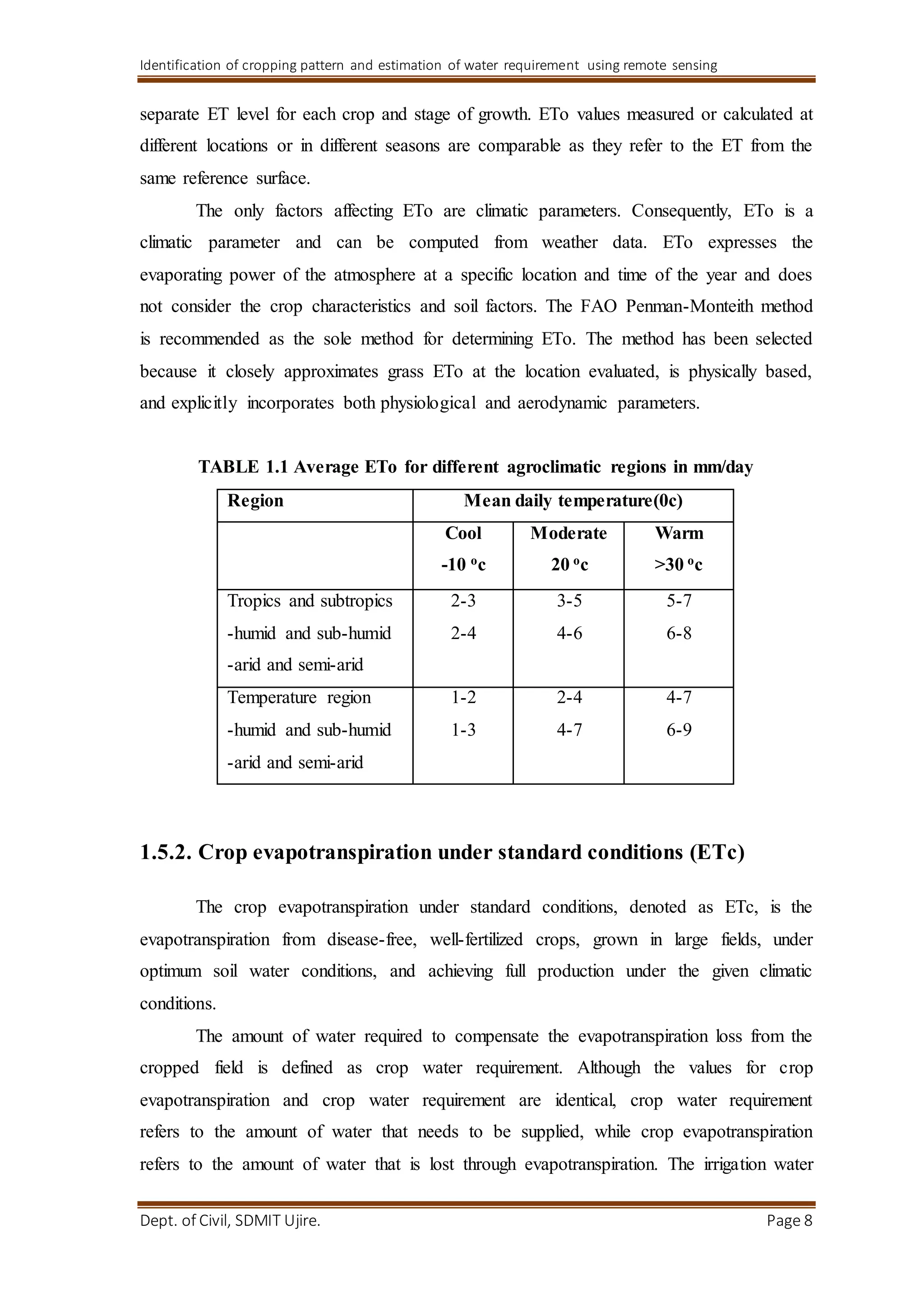
World Meteorological Organization, to review the FAO methodologies on crop water
requirements and to advise on the revision and update of procedures.
The panel of experts recommended the adoption of the Penman-Monteith
combination method as a new standard for reference evapotranspiration and advised on
procedures for calculation of the various parameters. By defining the reference crop as a
hypothetical crop with an assumed height of 0.12 m having a surface resistance of 70 s m-
1 and an albedo of 0.23, closely resembling the evaporation of an extension surface of
green grass of uniform height, actively growing and adequately watered, the FAO
Penman-Monteith method was developed.
The FAO Penman-Monteith method to estimate ETo can be given as:
where ETo reference evapotranspiration [mm day-1],
Rn net radiation at the crop surface [MJ m-2 day-1],
G soil heat flux density [MJ m-2 day-1],
T mean daily air temperature at 2 m height [°C],
u2 wind speed at 2 m height [m s-1],
es saturation vapour pressure [kPa],
ea actual vapour pressure [kPa],
es-ea saturation vapour pressure deficit [kPa],
Δ slope vapour pressure curve [kPa °C-1],
γ psychrometric constant [kPa °C-1].
The reference evapotranspiration, ETo, provides a standard to which:
evapotranspiration at different periods of the year or in other regions can be compared
evapotranspiration of other crops can be related.
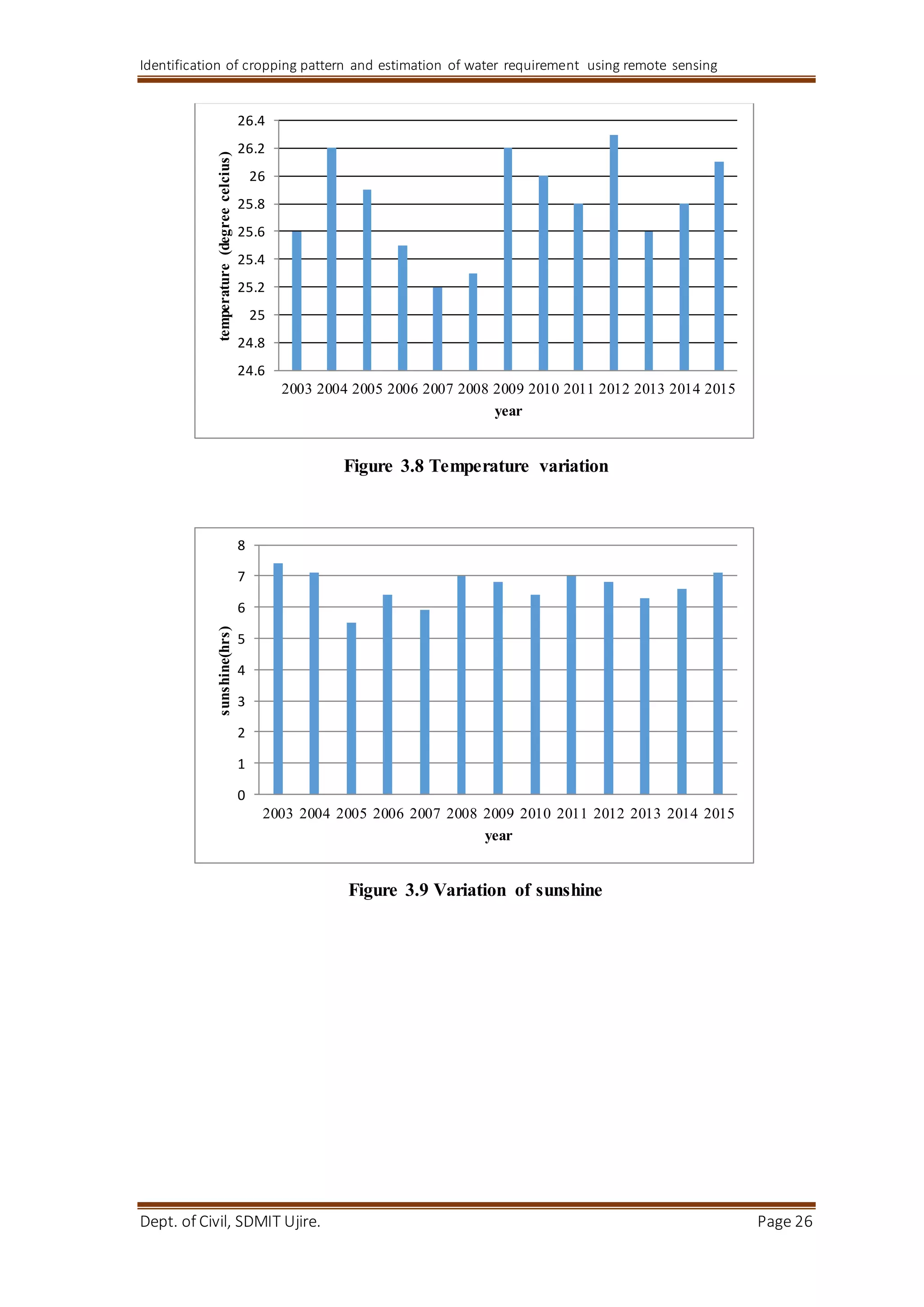
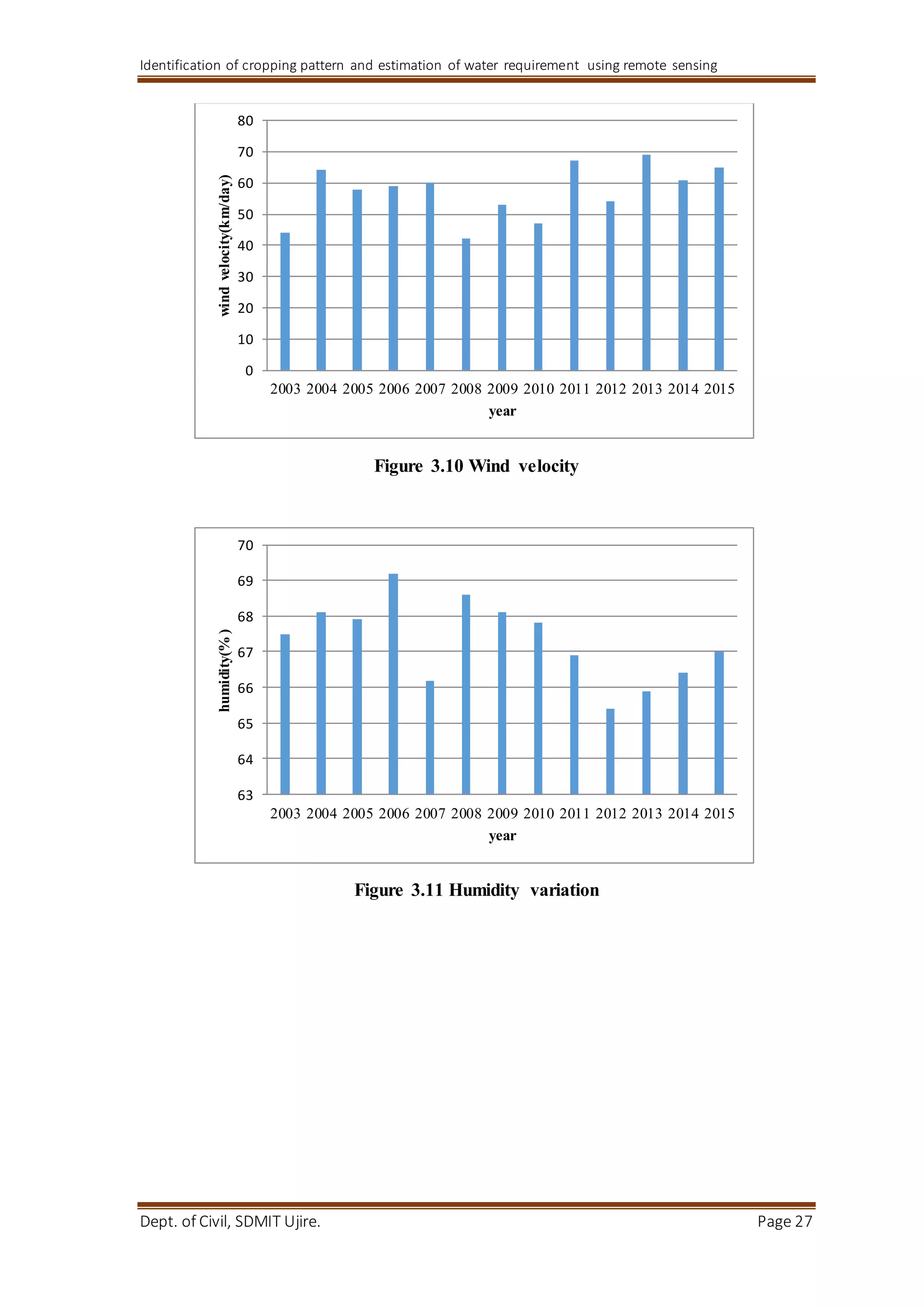
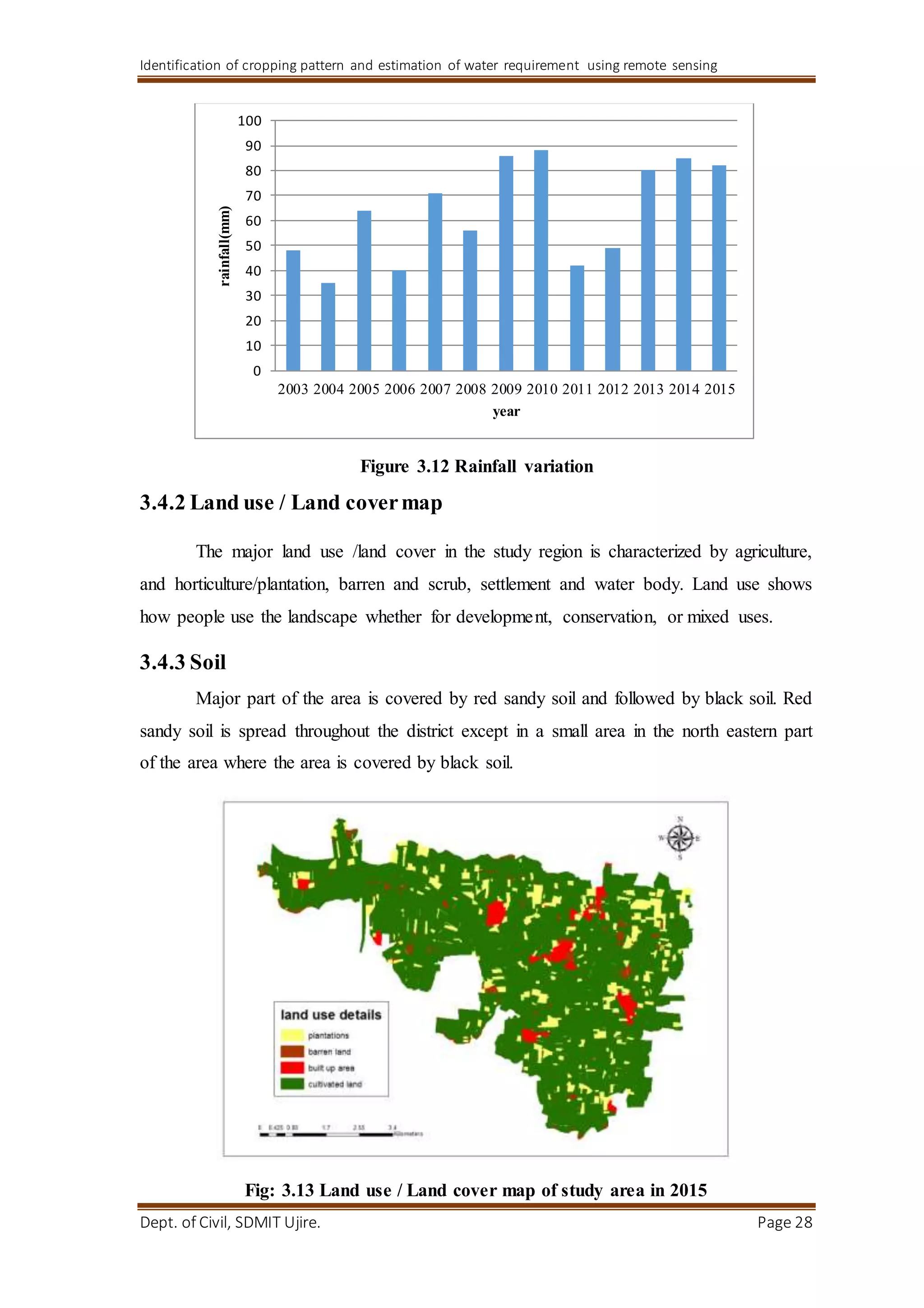
The equation uses standard climatological records of solar radiation (sunshine), air
temperature, humidity and wind speed.
The FAO Penman-Monteith equation is a close, simple representation of the
physical and physiological factors governing the evapotranspiration process. By using the
FAO Penman- Monteith definition for ETo, one may calculate crop coefficients at
32. Identification of cropping pattern and estimation of water requirement using remote sensing
Dept. of Civil, SDMIT Ujire. Page 32
research sites by relating the measured crop evapotranspiration (ETc) with the calculated
ETo, i.e., Kc = ETc/ETo.
4.1.3 MeterologicalData
The methods for calculating evapotranspiration from meteorological data require
various climatological and physical parameters. Some of the data are measured directly in
weather stations. Other parameters are related to commonly measured data and can be
derived with the help of a direct or empirical relationship.
Altitude above sea level (m) and latitude (degrees north or south) of the location
should be specified. These data are needed to adjust some weather parameters for the
local average value of atmospheric pressure (a function of the site elevation above mean
sea level) and to compute extraterrestrial radiation (Ra) and, in some cases, daylight hours
(N). In the calculation procedures for Ra and N, the latitude is expressed in radian (i.e.,
decimal degrees times π/180). A positive value is used for the northern hemisphere and a
negative value for the southern hemisphere.
4.1.4 MeteorologicalFactorsDetermining ET
The meteorological factors determining evapotranspiration are weather parameters
which provide energy for vaporization and remove water vapour from the evaporating
surface. The principal weather parameters to consider are presented below.
4.1.4.1Solarradiation
The evapotranspiration process is determined by the amount of energy available to
vaporize water. Solar radiation is the largest energy source and is able to change large
quantities of liquid water into water vapour. The potential amount of radiation that can
reach the evaporating surface is determined by its location and time of the year.
4.1.4.2. Air temperature
The solar radiation absorbed by the atmosphere and the heat emitted by the earth
increase the air temperature. The sensible heat of the surrounding air transfers energy to
the crop and exerts as such a controlling influence on the rate of evapotranspiration. In
sunny, warm weather the loss of water by evapotranspiration is greater than in cloudy and
cool weather.
33. Identification of cropping pattern and estimation of water requirement using remote sensing
Dept. of Civil, SDMIT Ujire. Page 33
4.1.4.3. Air humidity
While the energy supply from the sun and surrounding air is the main driving
force for the vaporization of water, the difference between the water vapour pressure at
the evapotranspiring surface and the surrounding air is the determining factor for the
vapour removal. In humid tropical regions, notwithstanding the high energy input, the
high humidity of the air will reduce the evapotranspiration demand. In such an
environment, the air is already close to saturation, so that less additional water can be
stored and hence the evapotranspiration rate is lower than in arid regions.
4.1.4.4. Wind speed
The process of vapour removal depends to a large extent on wind and air
turbulence which transfers large quantities of air over the evaporating surface. When
vaporizing water, the air above the evaporating surface becomes gradually saturated with
water vapour. If this air is not continuously replaced with drier air, the driving force for
water vapour removal and the evapotranspiration rate decreases.
4.1.5. Atmospheric Parameters
Several relationships are available to express climatic parameters. The effect of
the principal weather parameters on evapotranspiration can be assessed with the help of
these equations.
4.1.5.1. Atmospheric pressure (P)
The atmospheric pressure, P, is the pressure exerted by the weight of the earth's
atmosphere. Evaporation at high altitudes is promoted due to low atmospheric pressure as
expressed in the psychrometric constant. The effect is, however, small and in the
calculation procedures, the average value for a location is sufficient. A simplification of
the ideal gas law, assuming 20°C for a standard atmosphere, can be employed to calculate
P:
Where
P atmospheric pressure [kPa],
z elevation above sea level [m].
34. Identification of cropping pattern and estimation of water requirement using remote sensing
Dept. of Civil, SDMIT Ujire. Page 34
4.1.5.2. Latentheat of vaporization (λ)
The latent heat of vaporization, λ, expresses the energy required to change a unit
mass of water from liquid to water vapour in a constant pressure and constant temperature
process. The value of the latent heat varies as a function of temperature. At a high
temperature, less energy will be required than at lower temperatures. As λ varies only
slightly over normal temperature ranges a single value of 2.45 MJ kg-1 is taken in the
simplification of the FAO Penman-Monteith equation. This is the latent heat for an air
temperature of about 20°C.
4.1.5.3. Psychrometric constant(γ)
The psychrometric constant, γ, is given by:
Where
γ psychrometric constant [kPa °C-1],
P atmospheric pressure [kPa],
γ latent heat of vaporization, 2.45 [MJ kg-1],
cp specific heat at constant pressure, 1.013×10⁻³ [MJ kg-1 °C-1],
λ ratio molecular weight of water vapour/dry air = 0.622.
The specific heat at constant pressure is the amount of energy required to increase
the temperature of a unit mass of air by one degree at constant pressure. Its value depends
on the composition of the air, i.e., on its humidity. For average atmospheric conditions a
value cp = 1.013 10-3 MJ kg-1 °C-1 can be used.
4.1.5.4Air Temperature
Agrometeorology is concerned with the air temperature near the level of the crop
canopy. Air temperature is measured with thermometers, thermistors or thermocouples.
Minimum and maximum thermometers record the minimum and maximum air
temperature over a 24-hour period. Thermographs plot the instantaneous temperature over
a day or week. Electronic weather stations often sample air temperature each minute and
report hourly averages in addition to 24-hour maximum and minimum values.
35. Identification of cropping pattern and estimation of water requirement using remote sensing
Dept. of Civil, SDMIT Ujire. Page 35
Due to the non-linearity of humidity data required in the FAO Penman-Monteith
equation, the vapour pressure for a certain period should be computed as the mean
between the vapour pressure at the daily maximum and minimum air temperatures of that
period. The daily maximum air temperature (Tmax) and daily minimum air temperature
(Tmin) are, respectively, the maximum and minimum air temperature observed during the
24-hour period, beginning at midnight. Tmax and Tmin for longer periods such as weeks,
10-day's or months are obtained by dividing the sum of the respective daily values by the
number of days in the period. The mean daily air temperature (Tmean) is only employed
in the FAO Penman-Monteith equation to calculate the slope of the saturation vapour
pressure curves (Δ) and the impact of mean air density (Pa) as the effect of temperature
variations on the value of the climatic parameter is small in these cases. For
standardization, Tmean for 24-hour periods is defined as the mean of the daily
maximum (Tmax) and minimum temperatures (Tmin) rather than as the average of
hourly temperature measurements.
The temperature is given in degrees Celsius(°C) or Fahrenheit (°F).
4.1.5.5Air Humidity
The water content of the air can be expressed in several ways. In
agrometeorology, vapour pressure, dew point temperature and relative humidity are
common expressions to indicate air humidity.
4.1.5.6. Vapour pressure
Water vapour is a gas and its pressure contributes to the total atmospheric
pressure. The amount of water in the air is related directly to the partial pressure exerted
by the water vapour in the air and is therefore a direct measure of the air water content.
In standard S.I. units, pressure is no longer expressed in centimetre of water, millimetre
of mercury, bars, atmosphere, etc., but in pascals (Pa).
When air is enclosed above an evaporating water surface, an equilibrium is reached
between the water molecules escaping and returning to the water reservoir. At that
moment, the air is said to be saturated since it cannot store any extra water molecules.
36. Identification of cropping pattern and estimation of water requirement using remote sensing
Dept. of Civil, SDMIT Ujire. Page 36
The corresponding pressure is called the saturation vapour pressure (eo(T) ). The number
of water molecules that can be stored in the air depends on the temperature (T).
The actual vapour pressure (ea) is the vapour pressure exerted by the water in the air.
When the air is not saturated, the actual vapour pressure will be lower than the saturation
vapour pressure. The difference between the saturation and actual vapour pressure is
called the vapour pressure deficit or saturation deficit and is an accurate indicator of the
actual evaporative capacity of the air.
4.1.5.7Dewpointtemperature
The dewpoint temperature is the temperature to which the air needs to be cooled
to make the air saturated. The actual vapour pressure of the air is the saturation vapour
pressure at the dewpoint temperature. The drier the air, the larger the difference between
the air temperature and dewpoint temperature.
4.1.5.8. Relative humidity
The relative humidity (RH) expresses the degree of saturation of the air as a ratio
of the actual (ea) to the saturation (eo(T)) vapour pressure at the same temperature (T):
Relative humidity is the ratio between the amount of water the ambient air
actually holds and the amount it could hold at the same temperature. It is dimensionless
and is commonly given as a percentage. Although the actual vapour pressure might be
relatively constant throughout the day, the relative humidity fluctuates between a
maximum near sunrise and a minimum around early afternoon. The variation of the
relative humidity is the result of the fact that the saturation vapour pressure is determined
by the air temperature. As the temperature changes during the day, the relative humidity
also changes substantially.
37. Identification of cropping pattern and estimation of water requirement using remote sensing
Dept. of Civil, SDMIT Ujire. Page 37
4.1.6 Calculationprocedures forair humidity
4.1.6.1. Meansaturationvapour pressure (es )
As saturation vapour pressure is related to air temperature, it can be calculated
from the air temperature. The relationship is expressed by:
Where
e°(T) saturation vapour pressure at the air temperature T [kPa],
T air temperature [°C],
Due to the non-linearity of the above equation, the mean saturation vapour
pressure for a day, week, decade or month should be computed as the mean between the
saturation vapour pressure at the mean daily maximum and minimum air temperatures for
that period:
Using mean air temperature instead of daily minimum and maximum temperatures
results in lower estimates for the mean saturation vapour pressure. The corresponding
vapour pressure deficit (a parameter expressing the evaporating power of the atmosphere)
will also be smaller and the result will be some underestimation of the reference crop
evapotranspiration. Therefore, the mean saturation vapour pressure should be calculated
as the mean between the saturation vapour pressure at both the daily maximum and
minimum air temperature.
4.1.6.2. Slope ofsaturation vapour pressure curve (Δ)
For the calculation of evapotranspiration, the slope of the relationship between
saturation vapour pressure and temperature, Δ, is required.
Where
Δ = slope of saturation vapour pressure curve at air temperature T [kPa °C1],
38. Identification of cropping pattern and estimation of water requirement using remote sensing
Dept. of Civil, SDMIT Ujire. Page 38
T = air temperature [°C],
In the FAO Penman-Monteith equation, where Δ occurs in the numerator and
denominator, the slope of the vapour pressure curve is calculated using mean air
temperature
4.1.6.3. Actual vapour pressure (ea ) derived from relative humidity
data
The actual vapour pressure can also be calculated from the relative humidity.
• For RHmean:
In the absence of RHmax and RHmin, this equation can be used to estimate ea:
where RHmean is the mean relative humidity, defined as the average between
RHmax and RHmin.
4.1.6.4. Vapour pressure deficit (es – ea )
The vapour pressure deficit is the difference between the saturation (es) and actual
vapour pressure (ea) for a given time period. For time periods such as a week, ten days or
a month es is computed from Equation 3.8 using the Tmax and Tmin averaged over the
time period and similarly the ea is computed with equation 4.10, using average
measurements over the period
4.1.7. Radiation
4.1.7.1Extraterrestrialradiation (Ra )
The radiation striking a surface perpendicular to the sun's rays at the top of the
earth's atmosphere, called the solar constant, is about 0.082 MJ m-2 min-1. The local
intensity of radiation is, however, determined by the angle between the direction of the
sun's rays and the normal to the surface of the atmosphere. This angle will change during
the day and will be different at different latitudes and in different seasons. The solar
39. Identification of cropping pattern and estimation of water requirement using remote sensing
Dept. of Civil, SDMIT Ujire. Page 39
radiation received at the top of the earth's atmosphere on a horizontal surface is called the
extraterrestrial (solar) radiation, Ra.
If the sun is directly overhead, the angle of incidence is zero and the
extraterrestrial radiation is 0.0820 MJ m-2 min-1. As seasons change, the position of the
sun, the length of the day and, hence, Ra change as well. Extraterrestrial radiation is thus
a function of latitude, date and time of day.
4.1.7.2Solaror shortwave radiation(Rs )
As the radiation penetrates the atmosphere, some of the radiation is scattered,
reflected or absorbed by the atmospheric gases, clouds and dust. The amount of radiation
reaching a horizontal plane is known as the solar radiation, Rs. Because the sun emits
energy by means of electromagnetic waves characterized by short wavelengths, solar
radiation is also referred to as shortwave radiation.
For a cloudless day, Rs is roughly 75% of extraterrestrial radiation. On a cloudy
day, the radiation is scattered in the atmosphere, but even with extremely dense cloud
cover, about 25% of the extraterrestrial radiation may still reach the earth's surface mainly
as diffuse sky radiation. Solar radiation is also known as global radiation, meaning that it
is the sum of direct shortwave radiation from the sun and diffuse sky radiation from all
upward angles.
4.1.7.3Relative shortwave radiation(Rs /Rso )
The relative shortwave radiation is the ratio of the solar radiation (Rs) to the clear-
sky solar radiation (Rso). Rs is the solar radiation that actually reaches the earth's surface
in a given period, while Rso is the solar radiation that would reach the same surface
during the same period but under cloudless conditions.
The relative shortwave radiation is a way to express the cloudiness of the
atmosphere; the cloudier the sky the smaller the ratio. The ratio varies between about 0.33
(dense cloud cover) and 1 (clear sky). In the absence of a direct measurement of Rn, the
relative shortwave radiation is used in the computation of the net long wave radiation.
4.1.7.4Relative sunshine duration (n/N)
The relative sunshine duration is another ratio that expresses the cloudiness of the
atmosphere. It is the ratio of the actual duration of sunshine, n, to the maximum possible
duration of sunshine or daylight hours N. In the absence of any clouds, the actual duration
40. Identification of cropping pattern and estimation of water requirement using remote sensing
Dept. of Civil, SDMIT Ujire. Page 40
of sunshine is equal to the daylight hours (n = N) and the ratio is one, while on cloudy
days n and consequently the ratio may be zero. In the absence of a direct measurement of
Rs, the relative sunshine duration, n/N, is often used to derive solar radiation from
extraterrestrial radiation.
As with extraterrestrial radiation, the daylength N depends on the position of the
sun and is hence a function of latitude and date.
4.1.7.5Albedo (α) and net solarradiation (Rns)
A considerable amount of solar radiation reaching the earth's surface is reflected.
The fraction, α, of the solar radiation reflected by the surface is known as the albedo. The
albedo is highly variable for different surfaces and for the angle of incidence or slope of
the ground surface. It may be as large as 0.95 for freshly fallen snow and as small as 0.05
for a wet bare soil. A green vegetation cover has an albedo of about 0.20-0.25. For the
green grass reference crop, α is assumed to have a value of 0.23.
The net solar radiation, Rns, is the fraction of the solar radiation Rs that is not reflected
from the surface. Its value is (1-α)Rs.
4.1.7.6. Netlongwave radiation(Rnl)
The solar radiation absorbed by the earth is converted to heat energy. By several
processes, including emission of radiation, the earth loses this energy. The earth, which is
at a much lower temperature than the sun, emits radiative energy with wavelengths longer
than those from the sun. Therefore, the terrestrial radiation is referred to as longwave
radiation. The emitted longwave radiation (R1,up) is absorbed by the atmosphere or is
lost into space. The longwave radiation received by the atmosphere (R1,down) increases
its temperature and, as a consequence, the atmosphere radiates energy of its own. Part of
the radiation finds it way back to the earth's surface. Consequently, the earth's surface
both emits and receives longwave radiation. The difference between outgoing and
incoming longwave radiation is called the net longwave radiation, Rnl. As the outgoing
longwave radiation is almost always greater than the incoming longwave radiation, Rnl
represents an energy loss.
41. Identification of cropping pattern and estimation of water requirement using remote sensing
Dept. of Civil, SDMIT Ujire. Page 41
4.1.7.7Netradiation (Rn)
The net radiation, Rn, is the difference between incoming and outgoing radiation
of both short and long wavelengths. It is the balance between the energy absorbed,
reflected and emitted by the earth's surface or the difference between the incoming net
shortwave (Rns) and the net outgoing longwave (Rnl) radiation (Figure 4.1). Rn is
normally positive during the daytime and negative during the nighttime. The total daily
value for Rn is almost always positive over a period of 24 hours, except in extreme
conditions at high latitudes.
Fig 4.1 various components of radiation
4.1.7.8. Soilheatflux (G)
In making estimates of evapotranspiration, all terms of the energy balance should
be considered. The soil heat flux, G, is the energy that is utilized in heating the soil. G is
positive when the soil is warming and negative when the soil is cooling. Although the soil
heat flux is small compared to Rn and may often be ignored, the amount of energy gained
or lost by the soil in this process should theoretically be subtracted or added to Rn when
estimating evapotranspiration.
42. Identification of cropping pattern and estimation of water requirement using remote sensing
Dept. of Civil, SDMIT Ujire. Page 42
4.1.8 Calculationprocedures forradiation
4.1.8.1. Extraterrestrialradiation(Ra)
The extraterrestrial radiation (Ra) value is calculated by selecting a value in
mm/day from Table 10 for given month and latitude of FAO Irrigation and Drainage
Paper No.24, as there were no sufficient data available for the equation suggested by FAO
Irrigation and Drainage Paper No.56.
4.1.8.2Solarradiation (Rs )
If the solar radiation, Rs, is not measured, it can be calculated with the Angstrom
formula,This relates solar radiation to extra-terrestrial radiation and relative sunshine
duration:
Where
Rs solar or shortwave radiation [MJ m-2 day-1],
n actual duration of sunshine [hour],
N maximum possible duration of sunshine or daylight hours [hour],
n/N relative sunshine duration [-],
Rs extraterrestrial radiation [MJ m-2 day-1],
as regression constant, expressing the fraction of extraterrestrial radiation
reaching the earth on overcast days (n = 0),
as+bs fraction of extraterrestrial radiation reaching the earth on clear days (n = N).
Rs is expressed in the above equation in MJ m-2 day-1. The corresponding
equivalent evaporation in mm day-1 is obtained by multiplying Rs by 0.408
Depending on atmospheric conditions (humidity, dust) and solar declination
(latitude and month), the Angstrom values as and bs will vary. Where no actual
solar radiation data are available and no calibration has been carried out for
improved as and bs parameters, the values as = 0.25 and bs = 0.50 are
recommended.
4.1.8.3Clear-skysolarradiation (Rso )
The calculation of the clear-sky radiation, Rso, when n = N, is required for computing net
long wave radiation.
43. Identification of cropping pattern and estimation of water requirement using remote sensing
Dept. of Civil, SDMIT Ujire. Page 43
• For near sea level or when calibrated values for as and bs are available:
Where
Rso clear-sky solar radiation [MJ m-2 day-1],
as+bs fraction of extraterrestrial radiation reaching the earth on clear-sky days
(n=N).
4.1.8.4Netsolaror net shortwave radiation (Rns )
The net shortwave radiation resulting from the balance between incoming and
reflected solar radiation is given by:
where
Rns = net solar or shortwave radiation [MJ m-2 day-1],
α = albedo or canopy reflection coefficient, which is 0.23 for the hypothetic grass
reference crop [dimensionless],
Rs = the incoming solar radiation [MJ m-2 day-1].
Rns is expressed in the above equation in MJ m-2 day-1.
4.1.8.5 Net longwave radiation (Rnl )
The rate of longwave energy emission is proportional to the absolute temperature
of the surface raised to the fourth power. This relation is expressed quantitatively by the
Stefan-Boltzmann law. As humidity and cloudiness play an important role, the Stefan-
Boltzmann law is corrected by these two factors when estimating the net outgoing flux of
longwave radiation. It is thereby assumed that the concentrations of the other absorbers
are constant:
where
Rnl net outgoing longwave radiation [MJ m-2 day-1],
σ Stefan-Boltzmann constant [ 4.903 10-9 MJ K-4 m-2 day-1],
44. Identification of cropping pattern and estimation of water requirement using remote sensing
Dept. of Civil, SDMIT Ujire. Page 44
Tmax,K maximum absolute temperature during the 24-hour period [K = °C
+273.16],
Tmin,K minimum absolute temperature during the 24-hour period [K = °C +
273.16],
ea actual vapour pressure [kPa],
Rs/Rso relative shortwave radiation (limited to ≤ 1.0),
Rs measured or calculated solar radiation [MJ m-2 day-1],
Rso calculated clear-sky radiation [MJ m-2 day-1].
An average of the maximum air temperature to the fourth power and the minimum air
temperature to the fourth power is commonly used in the Stefan-Boltzmann equation for
24- hour time steps. The term (0.34-0.14√ea) expresses the correction for air humidity,
and will be smaller if the humidity increases. The effect of cloudiness is expressed by
(1.35 Rs/Rso - 0.35). The term becomes smaller if the cloudiness increases and hence Rs
decreases. The smaller the correction terms, the smaller the net outgoing flux of longwave
radiation. Note that the Rs/Rso term in Equation 3.17 must be limited so that Rs/Rso ≤
1.0.
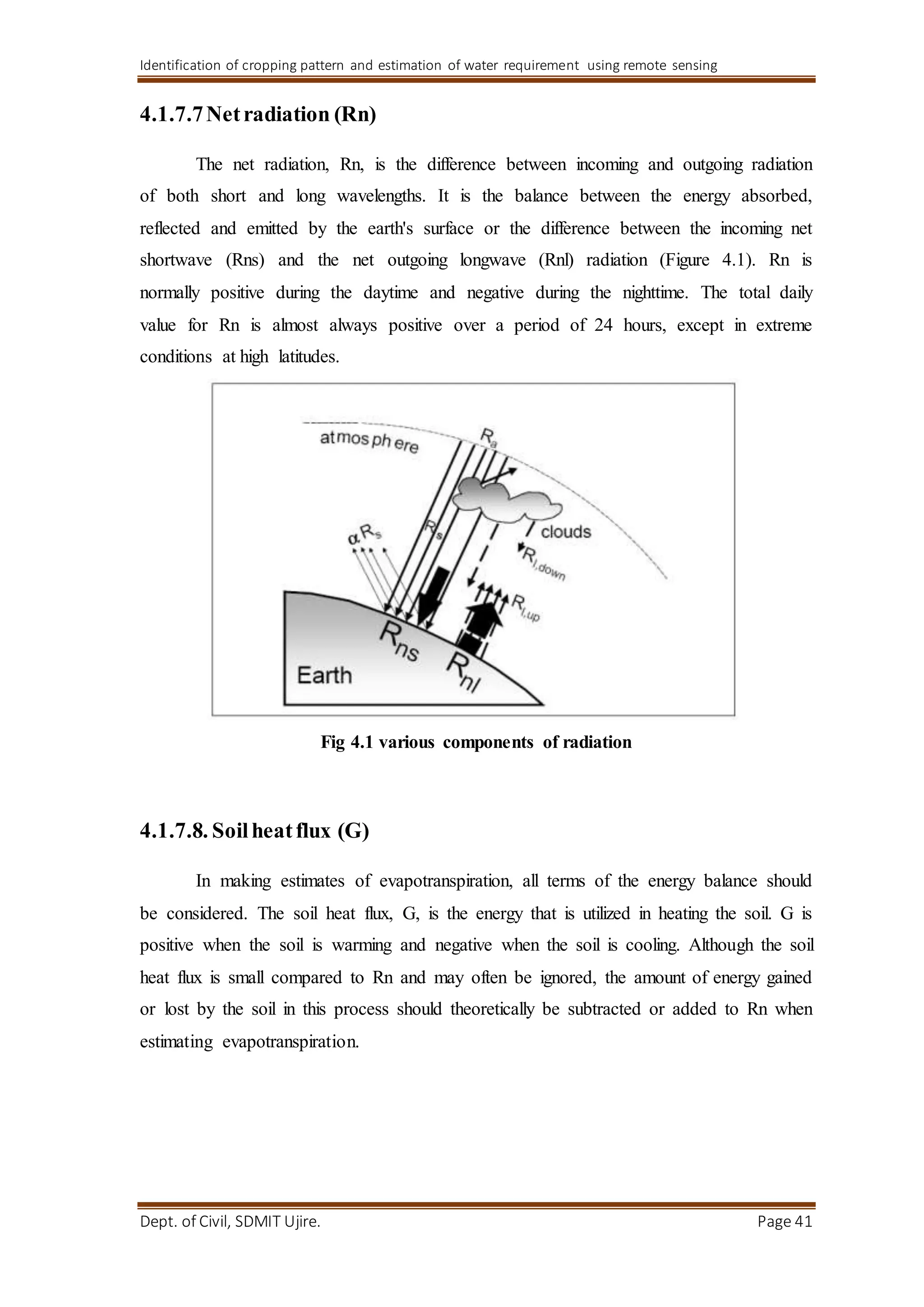
4.1.8.6Netradiation (Rn )
The net radiation (Rn) is the difference between the incoming net shortwave
radiation (Rns)
and the outgoing net longwave radiation (Rnl):
As the magnitude of the day or ten-day soil heat flux beneath the grass reference surface
is relatively small, it may be ignored
4.1.9 Actual evapotranspiration:
Actual evapotranspiration is calculated by multiplying crop coefficient with the
reference evapotranspiration. It is given by
where
ETc crop evapotranspiration [mm d-1],
Kc crop coefficient [dimensionless],
45. Identification of cropping pattern and estimation of water requirement using remote sensing
Dept. of Civil, SDMIT Ujire. Page 45
ETo reference crop evapotranspiration [mm d-1]
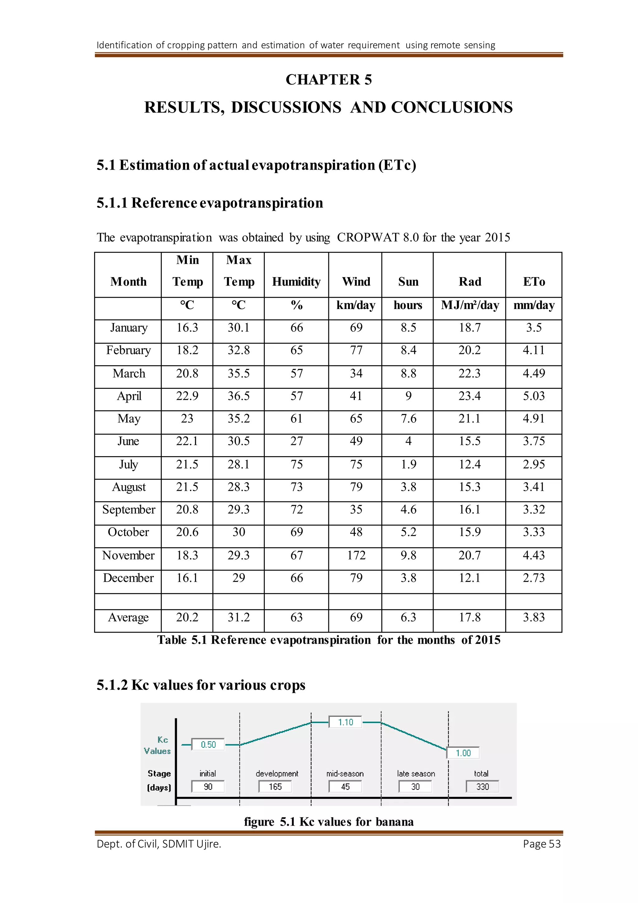
Month
Min
Temp
Max
Temp Humidity Wind Sun Rain
°C °C % km/day hours Mm
January 16.3 30.1 66 69 8.5 0
February 18.2 32.8 65 77 8.4 0
March 20.8 35.5 57 34 8.8 21.2
April 22.9 36.5 57 41 9 25.2
May 23 35.2 61 65 7.6 115
June 22.1 30.5 27 49 4 89.2
July 21.5 28.1 75 75 1.9 153.6
August 21.5 28.3 73 79 3.8 99.2
September 20.8 29.3 72 35 4.6 330.2
October 20.6 30 69 48 5.2 105.2
November 18.3 29.3 67 172 9.8 26.2
December 16.1 29 66 79 3.8 0
Table 4.1 Hydrometeorological data for 2015
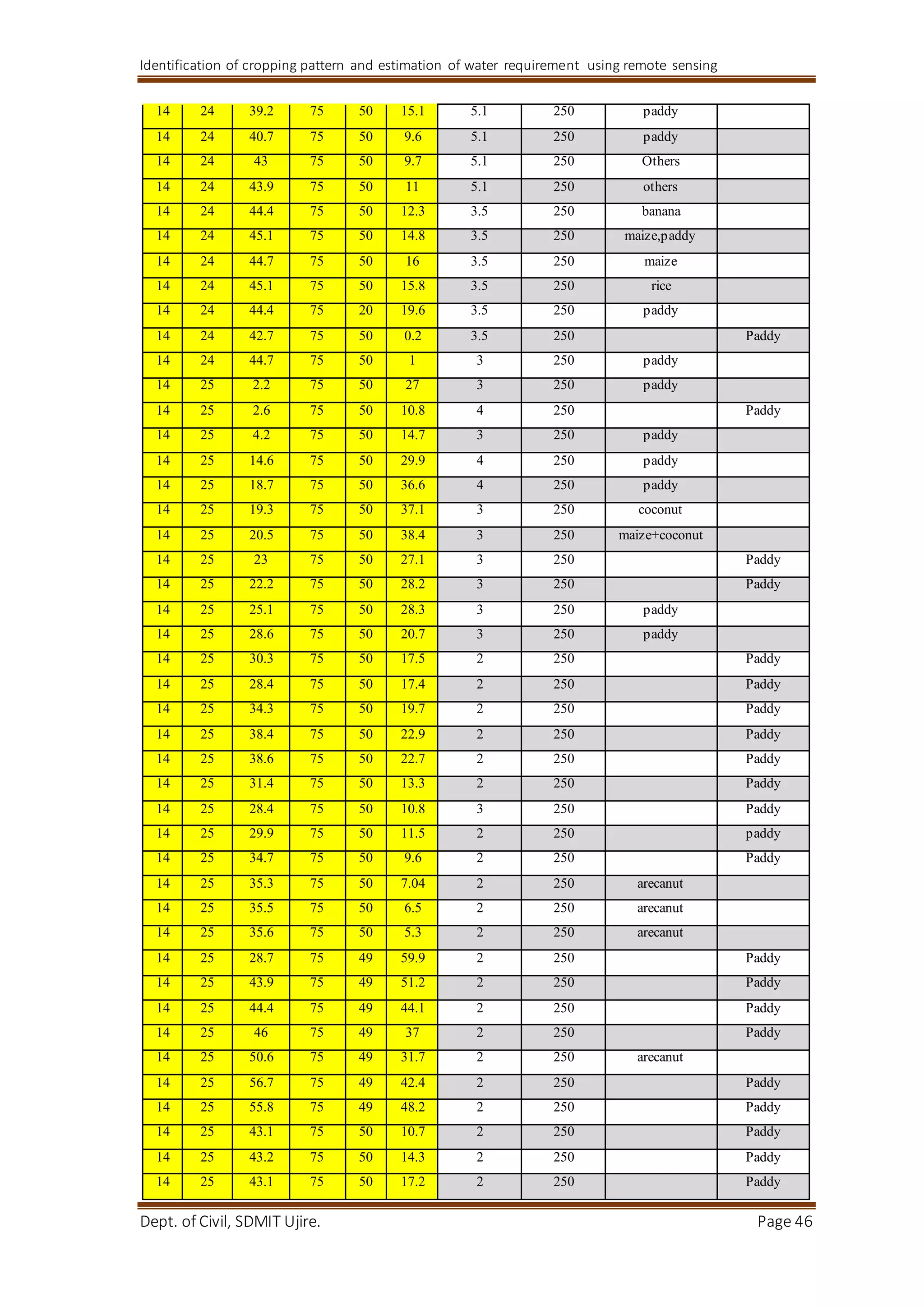
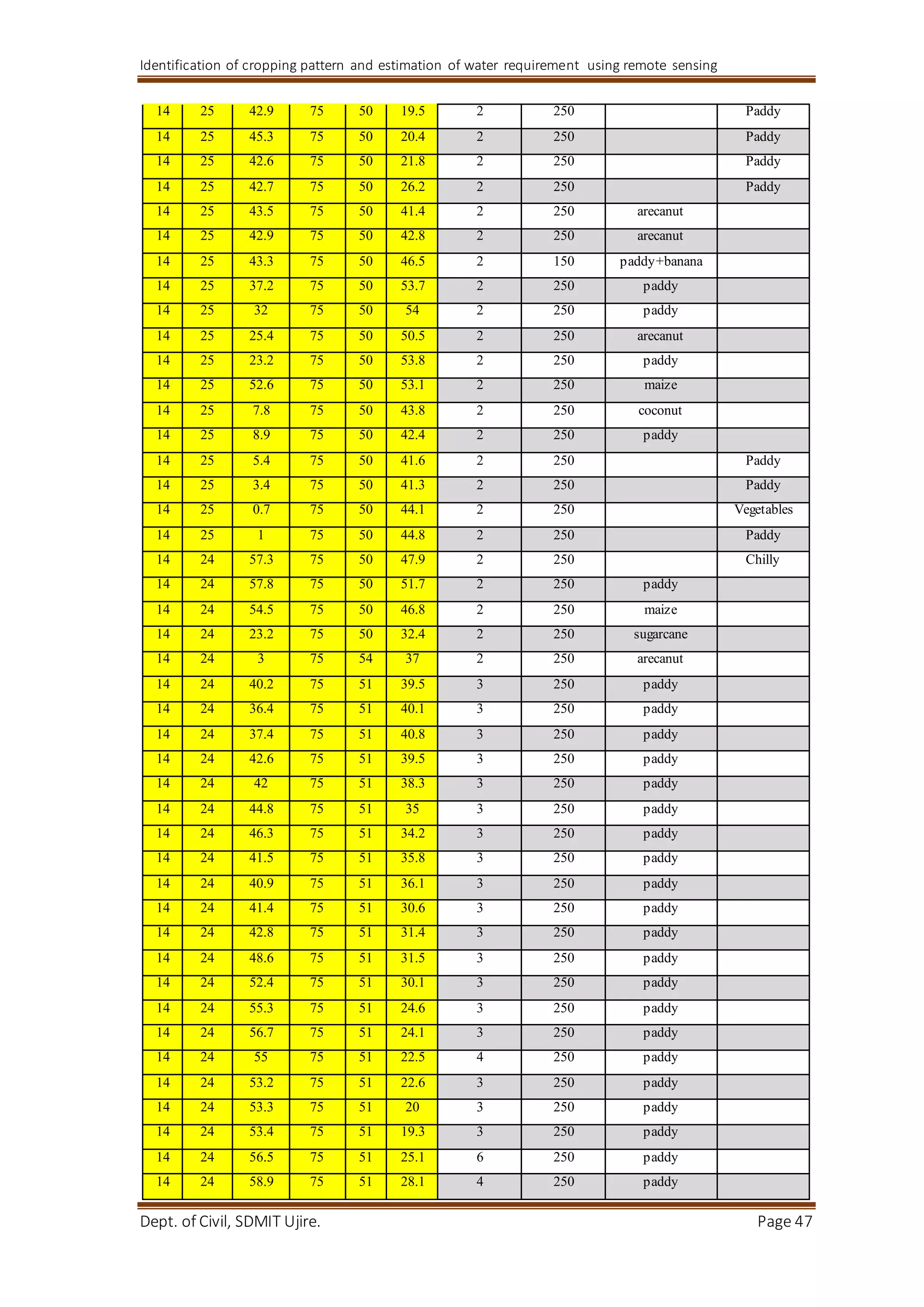
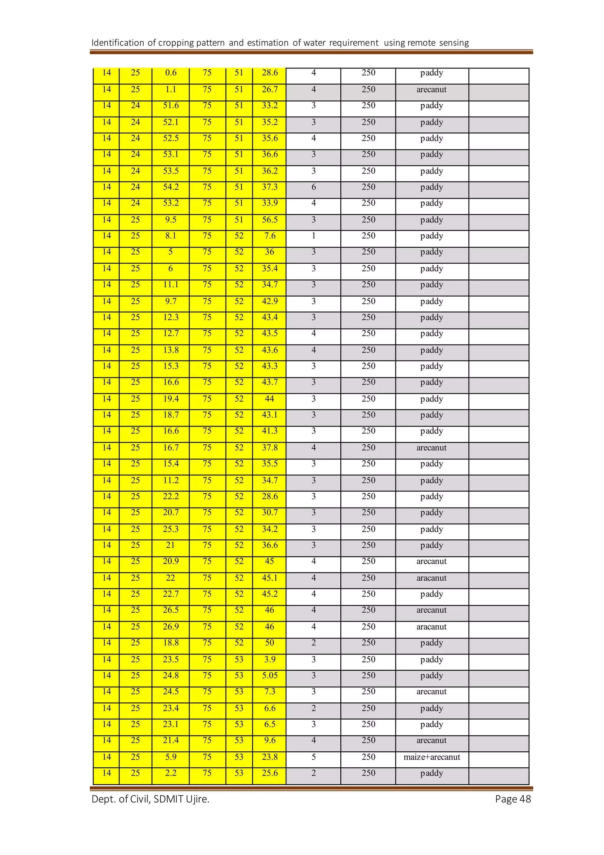
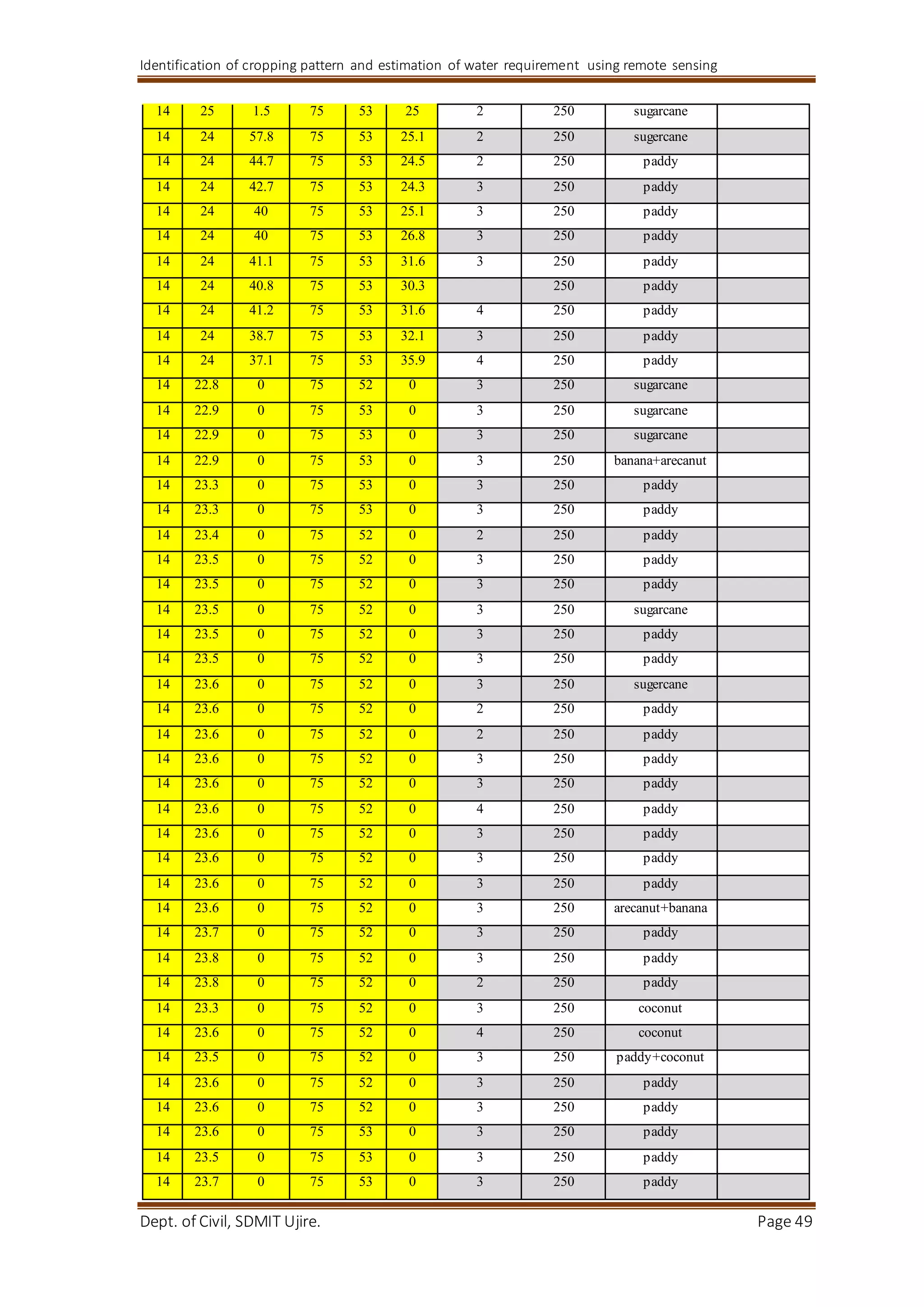
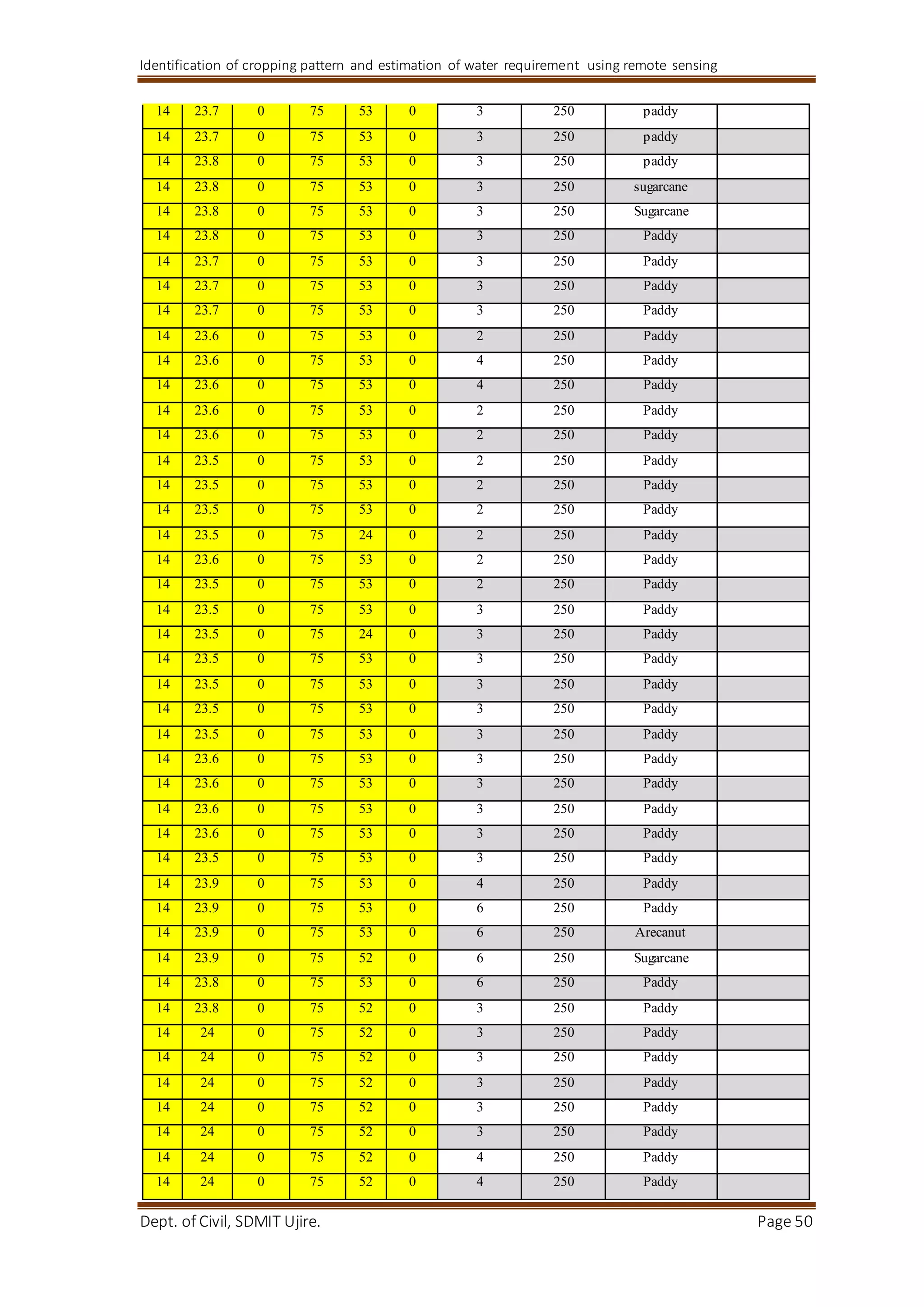
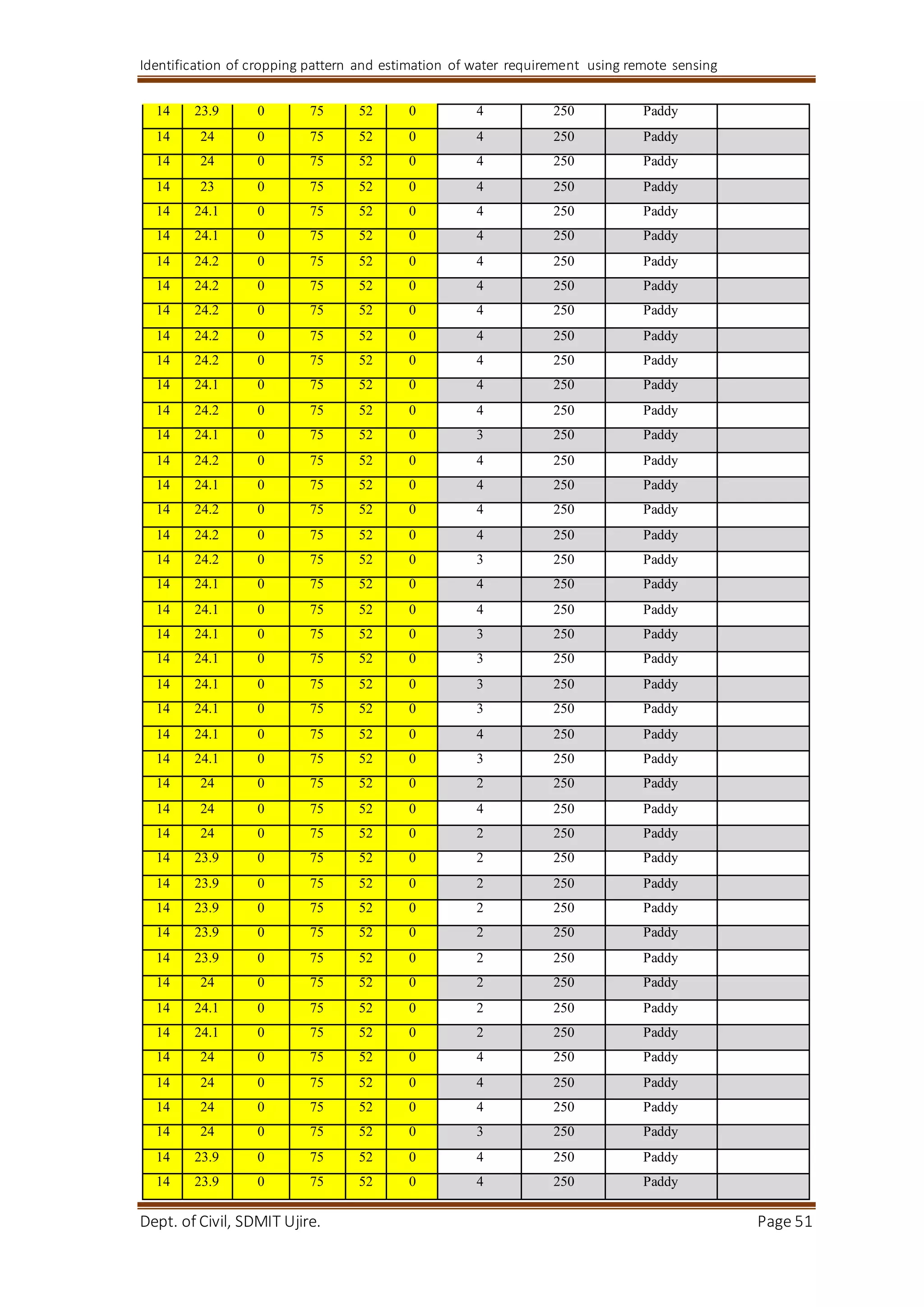
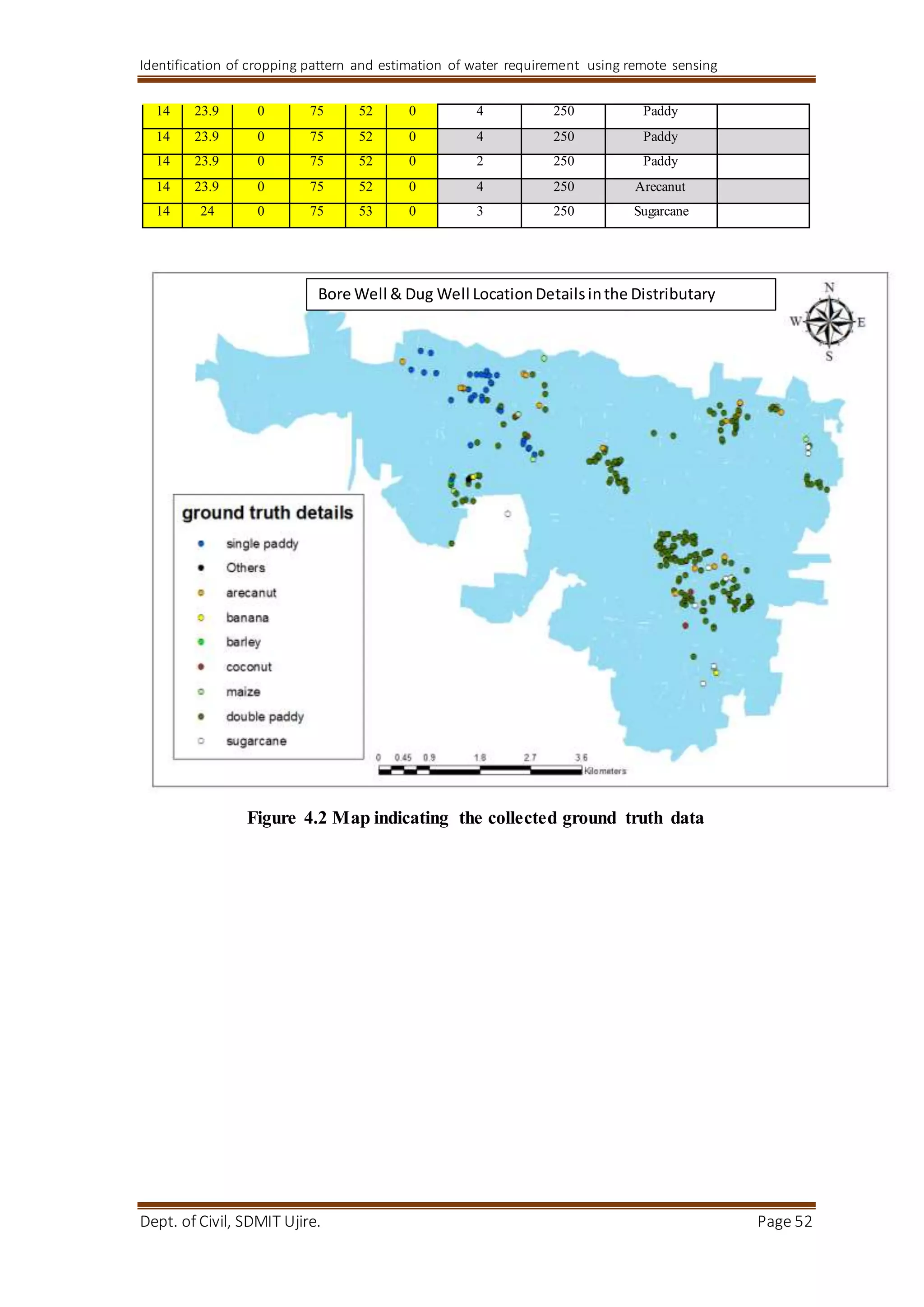
4.2 Estimation of cropping pattern
The identification of cropping pattern was done using ARC GIS 10.1 supervised
classification was carried out. Training samples were prepared using the ground truth data
that was collected in the field the following ground truth data was collected in the field in
2015
Latitude N Longitude E Borewell
Dia
Borewell
Depth
Double Crop Single Crop
14 24 30.5 75 50 12.4 3.5 250 paddy
14 24 31.3 75 50 8.4 3.5 250 paddy
14 24 30.5 75 50 6.3 3.5 250 paddy
14 24 6.15 75 50 0.17 3 250 paddy
14 24 39.6 75 49 59.7 3 250 paddy
14 24 41.3 75 49 59.7 3 250 barley
14 24 36.4 75 50 1.2 3 250 maize
14 24 34.7 75 50 3 4.5 250 paddy
14 24 28.8 75 50 2 4.5 250 paddy
52. Identification of cropping pattern and estimation of water requirement using remote sensing
Dept. of Civil, SDMIT Ujire. Page 52
14 23.9 0 75 52 0 4 250 Paddy
14 23.9 0 75 52 0 2 250 Paddy
14 23.9 0 75 52 0 4 250 Arecanut
14 24 0 75 53 0 3 250 Sugarcane
Figure 4.2 Map indicating the collected ground truth data
Bore Well & Dug Well LocationDetailsinthe Distributary
53. Identification of cropping pattern and estimation of water requirement using remote sensing
Dept. of Civil, SDMIT Ujire. Page 53
CHAPTER 5
RESULTS, DISCUSSIONS AND CONCLUSIONS
5.1 Estimation of actualevapotranspiration (ETc)
5.1.1 Referenceevapotranspiration
The evapotranspiration was obtained by using CROPWAT 8.0 for the year 2015
Month
Min
Temp
Max
Temp Humidity Wind Sun Rad ETo
°C °C % km/day hours MJ/m²/day mm/day
January 16.3 30.1 66 69 8.5 18.7 3.5
February 18.2 32.8 65 77 8.4 20.2 4.11
March 20.8 35.5 57 34 8.8 22.3 4.49
April 22.9 36.5 57 41 9 23.4 5.03
May 23 35.2 61 65 7.6 21.1 4.91
June 22.1 30.5 27 49 4 15.5 3.75
July 21.5 28.1 75 75 1.9 12.4 2.95
August 21.5 28.3 73 79 3.8 15.3 3.41
September 20.8 29.3 72 35 4.6 16.1 3.32
October 20.6 30 69 48 5.2 15.9 3.33
November 18.3 29.3 67 172 9.8 20.7 4.43
December 16.1 29 66 79 3.8 12.1 2.73
Average 20.2 31.2 63 69 6.3 17.8 3.83
Table 5.1 Reference evapotranspiration for the months of 2015
5.1.2 Kc values for various crops
figure 5.1 Kc values for banana
54. Identification of cropping pattern and estimation of water requirement using remote sensing
Dept. of Civil, SDMIT Ujire. Page 54
Figure 5.2 Kc values for maize
Figure 5.3 Kc values for rice
Figure 5.4 Kc values for sugarcane
5.1.3 Actual evapotranspirationfor various crops (ETc)
crop Etc(mm)
banana 944.7
maize 442.5
rice rabi 634.1
rice khariff 546.5
sugarcane 1375.8
arecanut 1532.87
coconut 1682
Table 5.2 Actual evapotranspiration (ETc) for year 2015
55. Identification of cropping pattern and estimation of water requirement using remote sensing
Dept. of Civil, SDMIT Ujire. Page 55
5.1.4 Irrigation requirement for various crops
crop Etc(mm) effective rain(mm) irrigation requirement(mm)
banana 944.7 610.4 582.5
maize 442.5 57.9 387.6
rice rabi 634.1 44.9 828.3
rice khariff 546.5 515.1 348
sugarcane 1375.8 685.2 820.1
arecanut 1532.87 685.2 847.67
coconut 1682 685.2 996.8
Table 5.3 Irrigation requirement for various crops
57. Identification of cropping pattern and estimation of water requirement using remote sensing
Dept. of Civil, SDMIT Ujire. Page 57
Figure 5.5 Google earth image of 10th distributary
5.2 Estimation of cropping pattern
Figure 5.6 LISS 3 NDVI image
58. Identification of cropping pattern and estimation of water requirement using remote sensing
Dept. of Civil, SDMIT Ujire. Page 58
Figure 5.7 Classified image obtained after supervised classification
Figure 5.8 Cropping pattern obtained after performing supervised classification
59. Identification of cropping pattern and estimation of water requirement using remote sensing
Dept. of Civil, SDMIT Ujire. Page 59
Land use Area(sqm)
Sugarcane 1225811.546
Single rice 4889876.297
Maize 737911.5978
Double rice 27445981.8
Coconut 841015.4332
Built up area 1418468.603
Barren land 731838.9495
Banana 2004747.776
arecanut 1454758.992
Table 5.5 Area covered by various crops and land use obtained by classified
map(figure 5.2)
Crop Notified area(hectares) Actual area(hectares) %violation
Rice 62.04 3233.5858 5112.098324
sugarcane 120.21 122.5811 1.972464853
plantations 1262.74 430.0521 65.94294154
Table 5.6 %Violation of cropping area by farmers
61. Identification of cropping pattern and estimation of water requirement using remote sensing
Dept. of Civil, SDMIT Ujire. Page 61
Figure 5.9 Graph showing irrigation requirement for the months of the year 2015
0
1000000
2000000
3000000
4000000
5000000
6000000
7000000
8000000
9000000
10000000
irrigationrequirement(cum/decade)
month
62. Identification of cropping pattern and estimation of water requirement using remote sensing
Dept. of Civil, SDMIT Ujire. Page 62
CHAPTER 6
CONCLUSIONS
1. Irrigation scheduling is the key element to proper management of irrigation system by
applying the correct amount of water at the right time to meet the requirement of water to
the plants.
2. From classification we can find huge violation of cropping area and because of that
shortage of supplied water in the tailrace. It’s clearly shows that there is proper water
management is required in the study area.
3. Scheduling efficiency was much lower for all treatments during the rainy summer
season compared to the other drier seasons indicating inaccuracy in determining site
specific rainfall.
4. Most crops will recover overnight from temporary wilting if less than 50 percent of the
plant available water has been depleted. Therefore, the allowable depletion volume
generally recommended is maximum 50 percent. However, the recommended volume
may range from 40 percent or less in sandy soils to more than 60 percent in clayey soils.
5. The allowable depletion is also dependent on the type of crop, its stage of development,
and its sensitivity to drought stress
6. When the irrigation scheduling is designed according to historical climate data or
estimated by computer program, it is important to look at the crop in the field for color
change or measuring soil water status to make sure that the estimation is right, because
this kind of scheduling does not take into account weather extremes which are different
from year to year.
Future scope of study
1. The same procedure can be carried out for other locations facing irrigation problems
2. Suitable irrigation scheduling can be developed to meet the deficit irrigation
requirement
63. Identification of cropping pattern and estimation of water requirement using remote sensing
Dept. of Civil, SDMIT Ujire. Page 63
REFERENCES
1. Allen, R.G., Pereira, L.S., Raes, D and Smith, M. (1990), FAO Irrigation and
Drainage Paper No. 56, Crop Evapotranspiration (guidelines for computing crop
water requirements). 300 p.
2. Annandale, J.G., Jovanovic, N.Z., Benade, N. and Allen, R.G. (2002) Software for
missing data error analysis of Penman-Monteith reference evapotranspiration. Irrg
Sci 21: 57-67.
3. Aruna Jyothy. S., Chandra Sekhar Reddy. K. and Mallikarjuna, P. (2011).
Development of Crop Coefficient Models for Weekly Crop Evapotranspiration
Estimation. ACEE, pp. 81-85.
4. A.W.Abdelhadi,Takeshi Hata(1999).Estimation of Crop Water requirements in
arid regions using P M equation with derived Crop coefficients.
5. Baburoa Kamble,Ayse Irmak, Kenneth Hubbard(2013).Estimating Crop
coeffecients using Remote Sensing based vegetation Index.
6. Doorenbos, J. and Puritt, W. O., (1977), FAO Irrigation and Drainage Paper No.
24, Guidelines for predicting crop water requirements. 144p.
7. Gaurav Pakhale, Prasun Gupta,Jyoti Nale(2010),Crop and Irrigation water
requirement estimation by Remote sensing and GIS.
8. K H V Durgarao,C S Krishna Kumar and V Hari Prasad(2001).Irrigaration water
requirements and Supply analysis in Dehradun Region-an Integrated Remote
Sensing GIS approach.
9. I.A.El-Magd and Tanton(2008) Remote Srnsing and GIS for estimation Crop
Water Demand.
10. Irmak, S., Haman, D.Z. and Jones, J.W. (2002). Evaluation of Class A Pan
Coefficients for Estimating Reference Evapotranspiration in Humid Location.
Journal of Irrigation and Drainage Engineering., ASCE, 128 (3): 153-159.
11. Isaya Kisekka, Kati W. Migliaccio, Michael D. Dukes, Jonathan H. Crane, and
Bruce Schaffer, (2010), Evapotranspiration-Based Irrigation for Agriculture: Crop
Coefficients of Some Commercial Crops in Florida, University of Florida, IFAS
Extension.
12. M.L. Chaudary and U.S. Kadam (2006), Micro-Irrigation for Cash Crops.
13. Mohammed A.En-Shirbeny,A-Elraouf M.Ali(2013).Crop Water requirements in
Egypt.
64. Identification of cropping pattern and estimation of water requirement using remote sensing
Dept. of Civil, SDMIT Ujire. Page 64
14. Nandagiri, L. and Kovoor G.M. (2005). Sensitivity of Food and Agriculture
Organization Penman-Monteith Evapotranspiration Estimates to Alternative
Procedures for Estimation of Parameters. Journal of Irrigation and Drainage
Engineering., ASCE, 131 (3): 238-248.
15. R.L. Snyder, M. Orang, K. Bali and S. Eching, Basic Irrigation Scheduling
(2000).
16. Rohitashw Kumar, Vijay Shankar and Mahesh Kumar. Modelling of Crop
Reference Evapotranspiration: A Review. Universal Journal of Environmental
Research and Technology, 1(3): 239-246.
17. S.Raut, K.S.S.Sharma, D K Das(2010).Study of Irrigation and crop water
requirements and growth of two Rabi Crops grown in a semi arid region using
Agrometeorology and Remote sensing.
18. Terry, T.A. and Dusek, D.A. (1994). Comparision of Vapor-Pressure-Decicit
Calculation Methods- Southern High Plains. Journal of Irrigation and Drainage
Engineering., ASCE, 121(2):191-198.
19. Water conservation Factsheet (2001), Crop Coefficients for use in Irrigation
Scheduling, British Columbia, Ministry of Agriculture, Food and Fisheries.