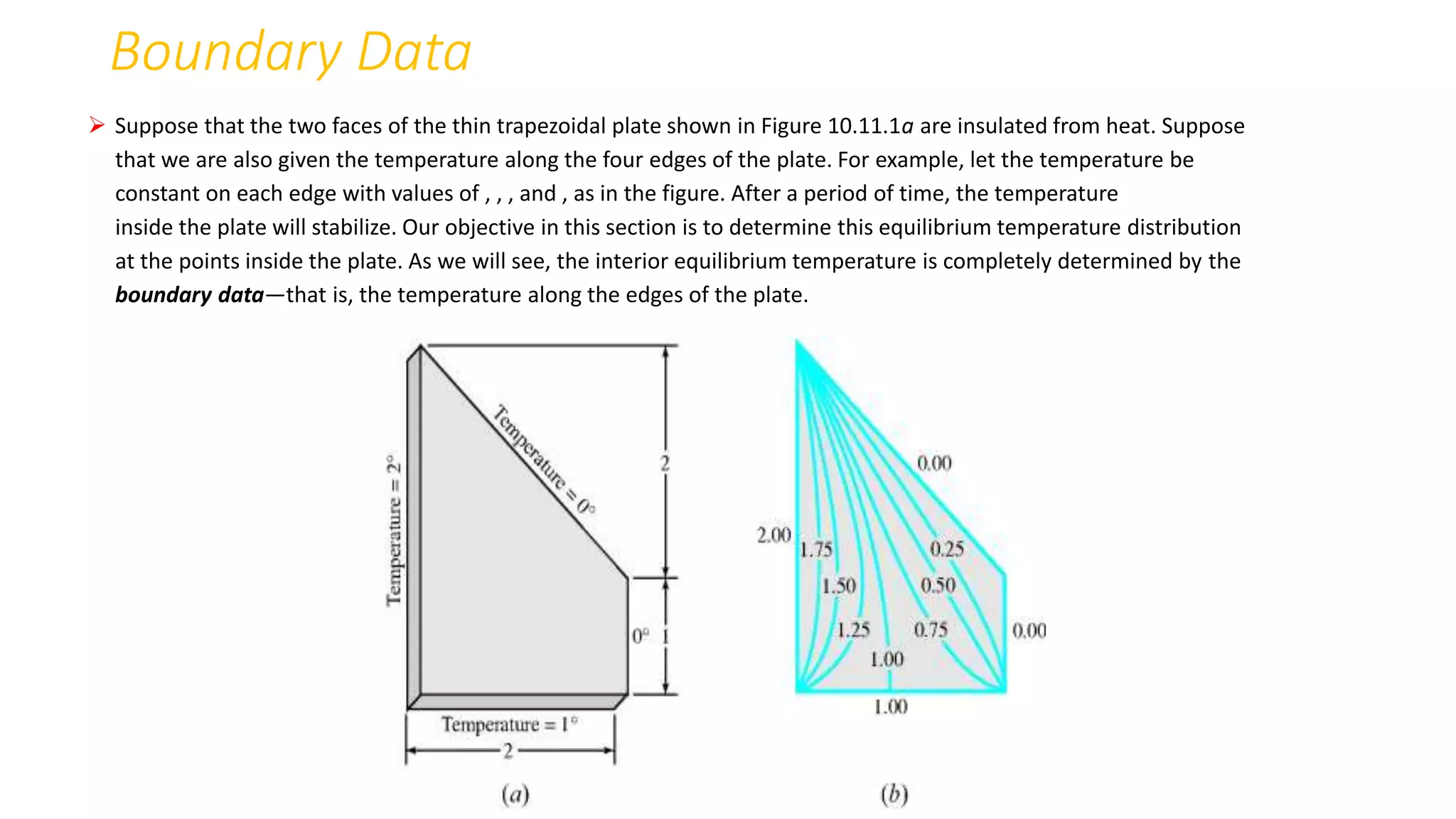
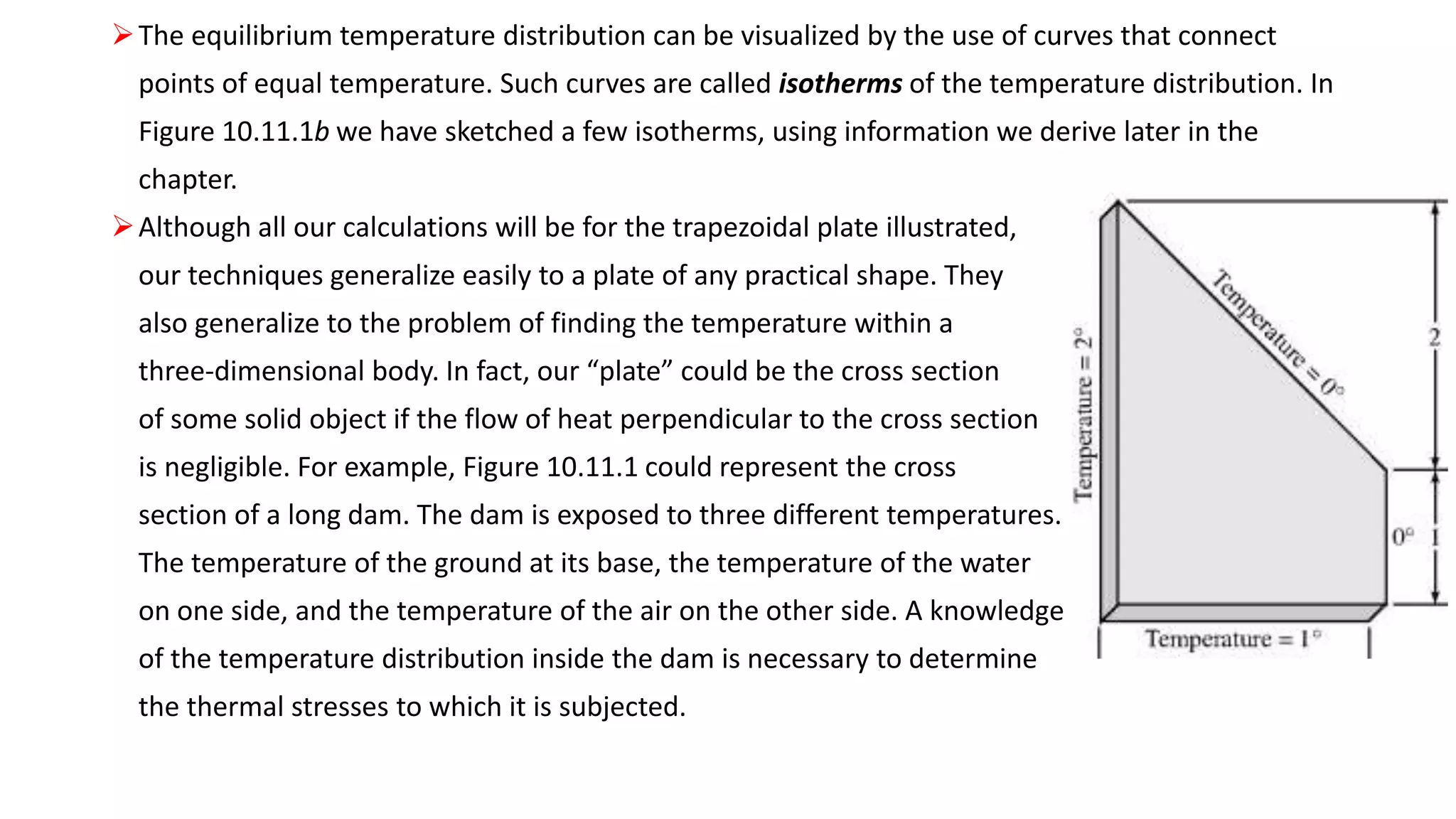
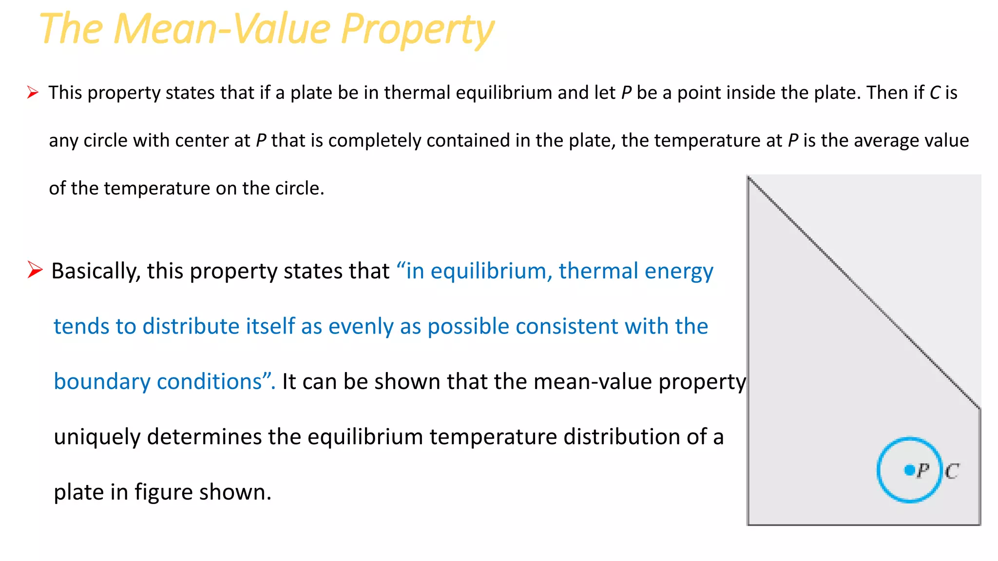
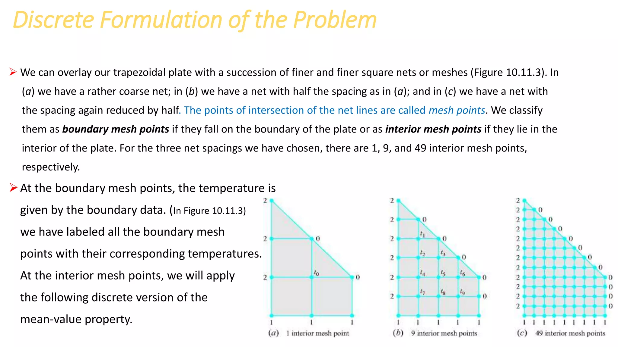
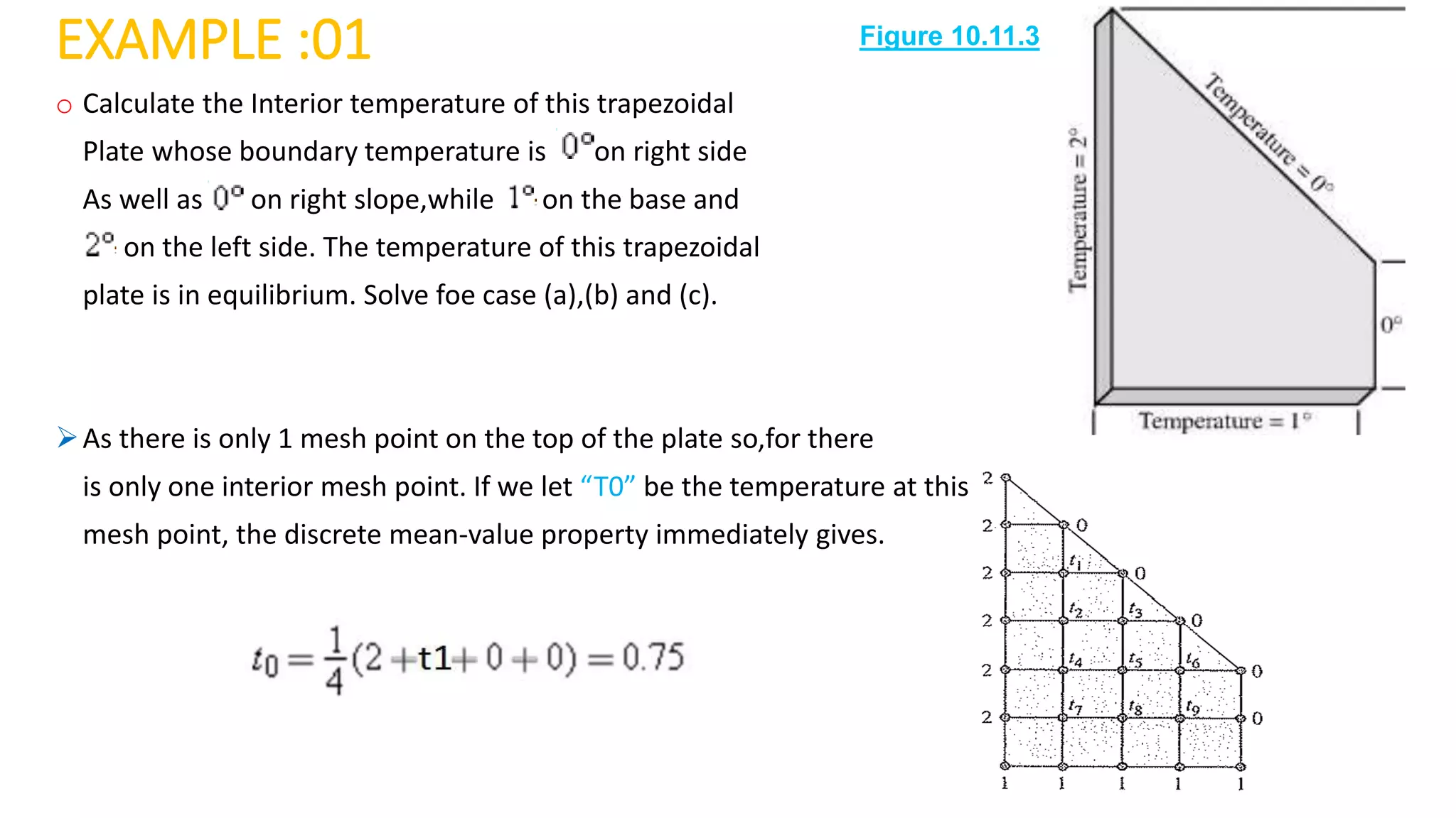
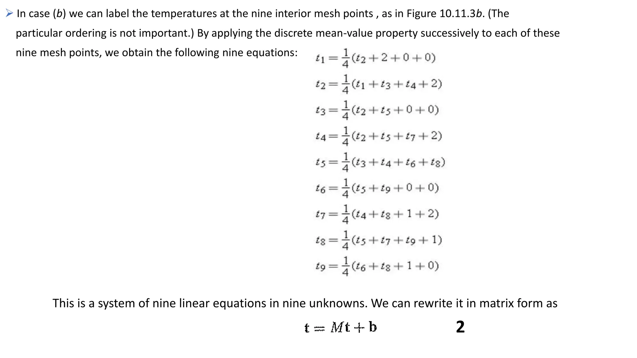
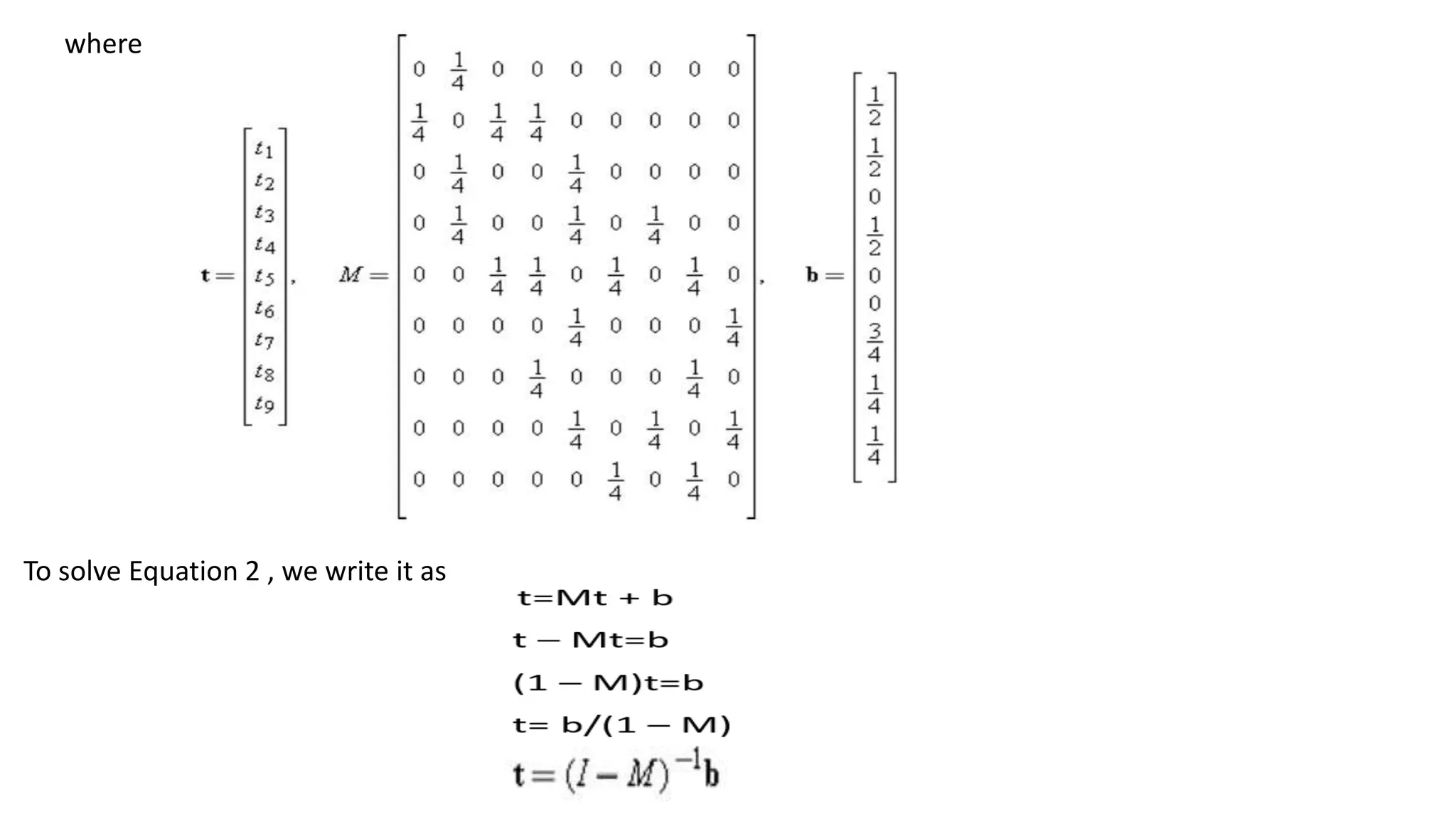
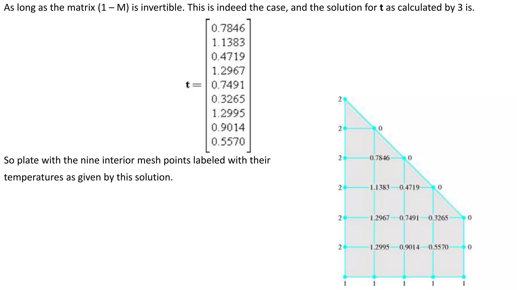
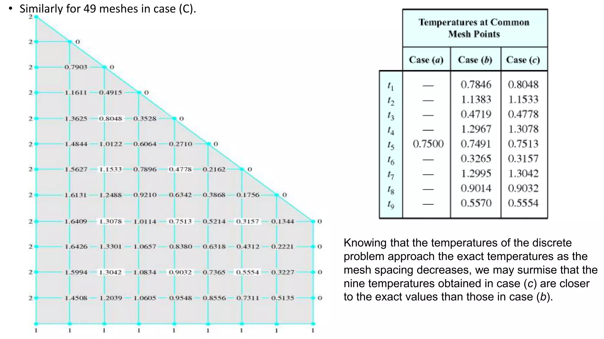
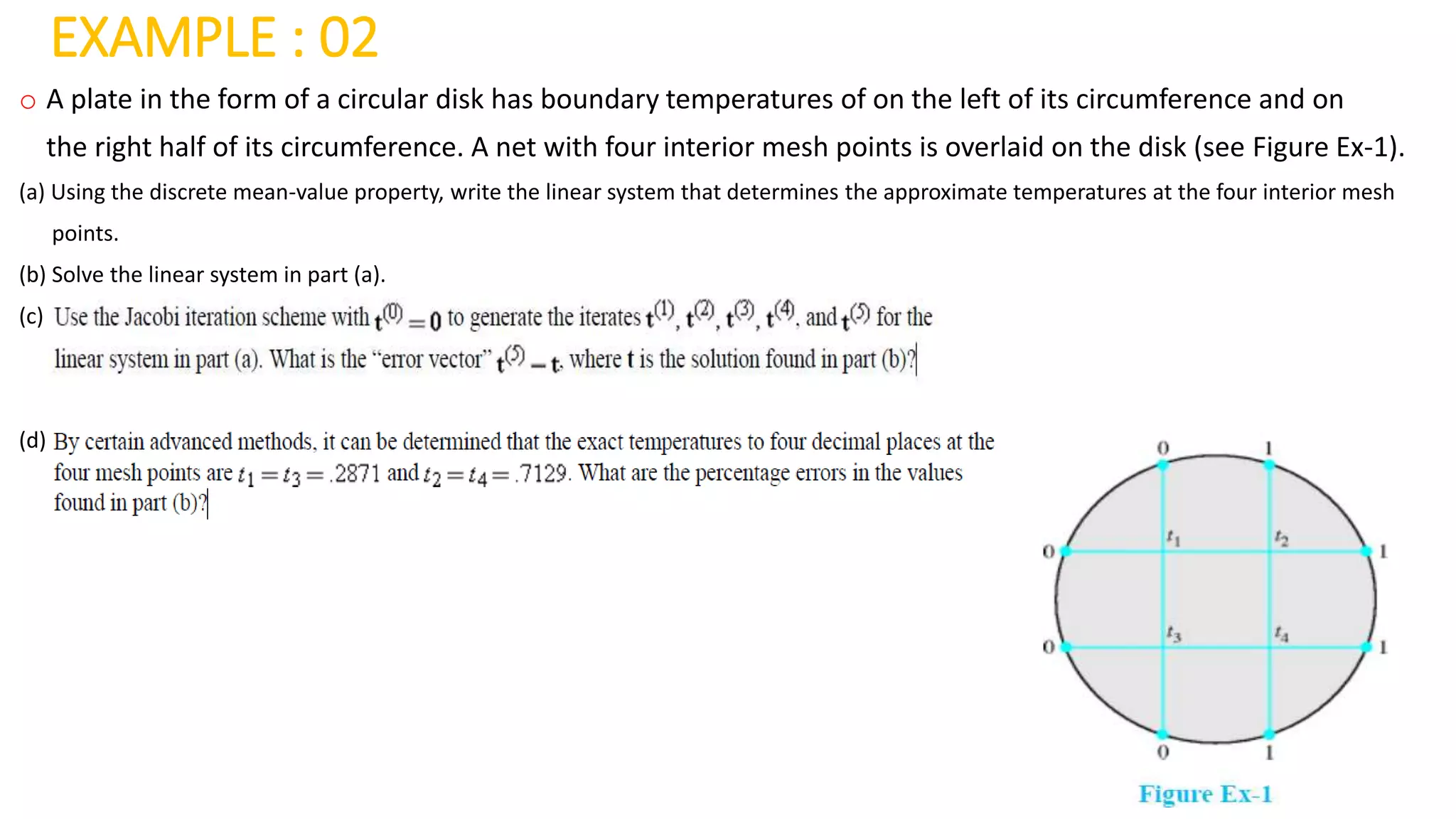
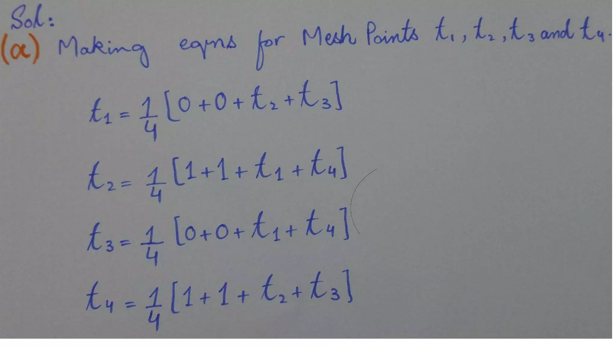
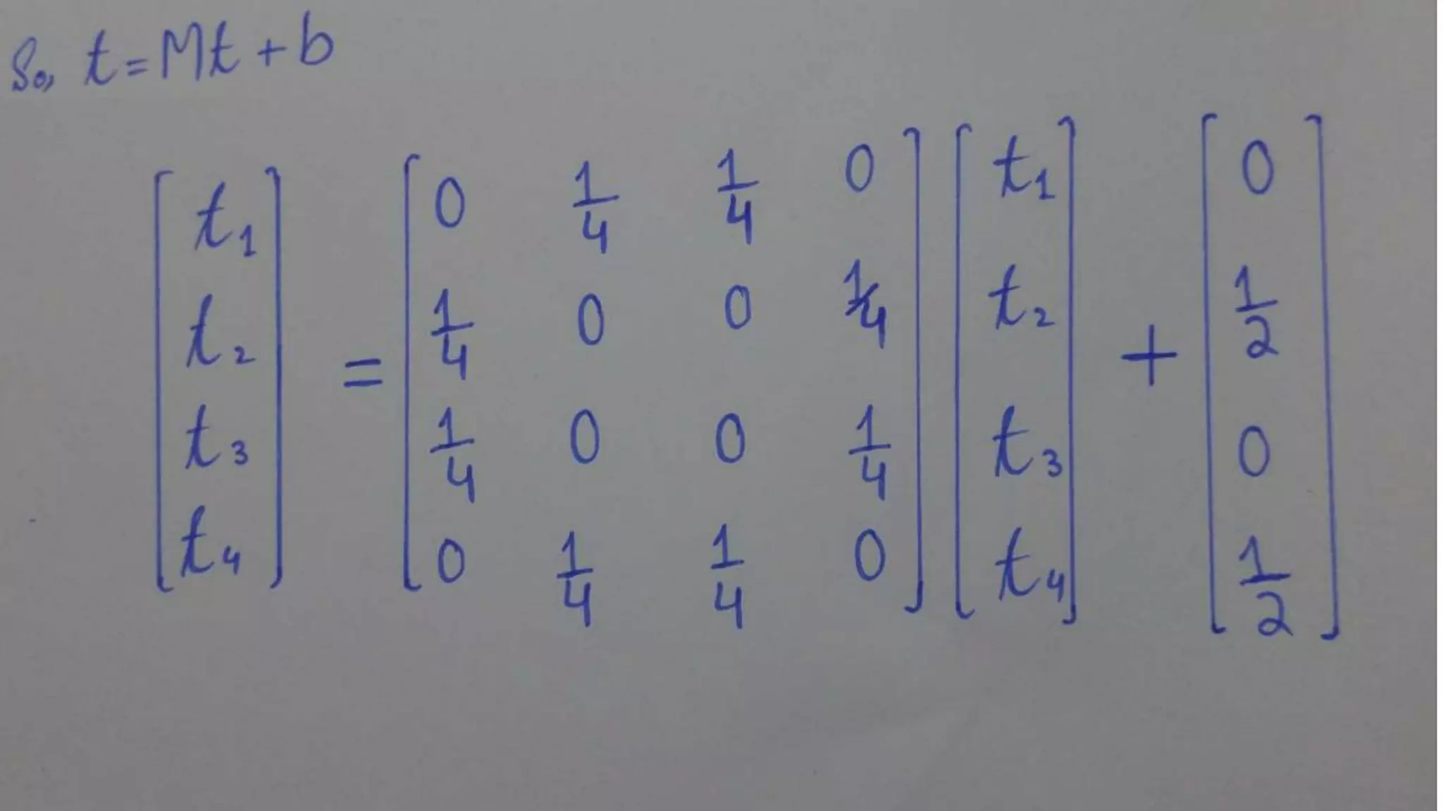
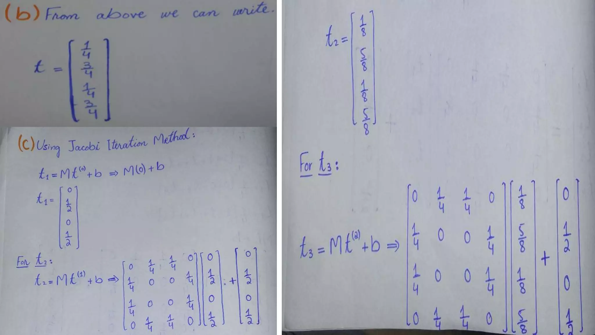
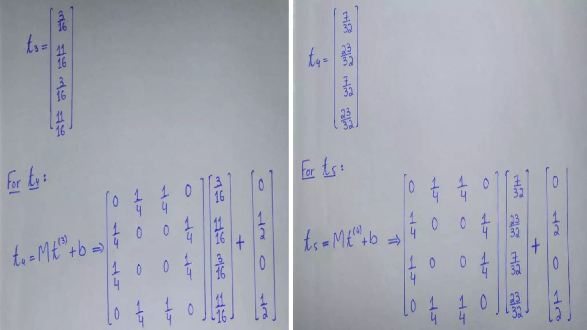
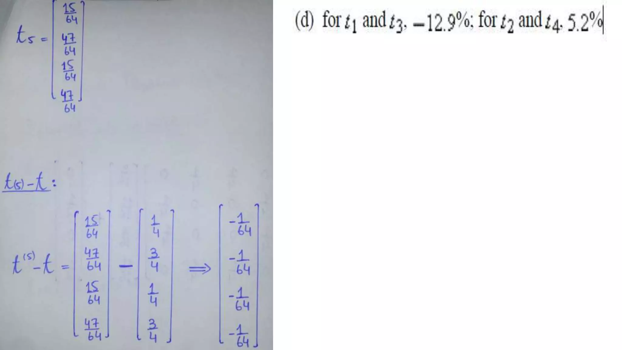
Call Girls In Bangalore ☎ 7737669865 🥵 Book Your One night Stand
Equilibrium Temperature Distributions Application In Linear Algebra
1. SEC-10.11: Equilibrium Temperature
Distributions
In this section we will see that the equilibrium temperature distribution within a trapezoidal plate can
be found when the temperatures around the edges of the plate are specified. The problem is reduced
to solving a system of linear equations by understanding the Mean Value Property of Thermal
Distributions in a uniform plate, and its discrete formulation as well.
Our goal is to be able to solve the following problems and explain the mathematics and the physics
in a form that would justify your solution to a classmate.
2. Boundary Data
Suppose that the two faces of the thin trapezoidal plate shown in Figure 10.11.1a are insulated from heat. Suppose
that we are also given the temperature along the four edges of the plate. For example, let the temperature be
constant on each edge with values of , , , and , as in the figure. After a period of time, the temperature
inside the plate will stabilize. Our objective in this section is to determine this equilibrium temperature distribution
at the points inside the plate. As we will see, the interior equilibrium temperature is completely determined by the
boundary data—that is, the temperature along the edges of the plate.
3. The equilibrium temperature distribution can be visualized by the use of curves that connect
points of equal temperature. Such curves are called isotherms of the temperature distribution. In
Figure 10.11.1b we have sketched a few isotherms, using information we derive later in the
chapter.
Although all our calculations will be for the trapezoidal plate illustrated,
our techniques generalize easily to a plate of any practical shape. They
also generalize to the problem of finding the temperature within a
three-dimensional body. In fact, our “plate” could be the cross section
of some solid object if the flow of heat perpendicular to the cross section
is negligible. For example, Figure 10.11.1 could represent the cross
section of a long dam. The dam is exposed to three different temperatures.
The temperature of the ground at its base, the temperature of the water
on one side, and the temperature of the air on the other side. A knowledge
of the temperature distribution inside the dam is necessary to determine
the thermal stresses to which it is subjected.
4. The Mean-Value Property
This property states that if a plate be in thermal equilibrium and let P be a point inside the plate. Then if C is
any circle with center at P that is completely contained in the plate, the temperature at P is the average value
of the temperature on the circle.
Basically, this property states that “in equilibrium, thermal energy
tends to distribute itself as evenly as possible consistent with the
boundary conditions”. It can be shown that the mean-value property
uniquely determines the equilibrium temperature distribution of a
plate in figure shown.
5. Discrete Formulation of the Problem
We can overlay our trapezoidal plate with a succession of finer and finer square nets or meshes (Figure 10.11.3). In
(a) we have a rather coarse net; in (b) we have a net with half the spacing as in (a); and in (c) we have a net with
the spacing again reduced by half. The points of intersection of the net lines are called mesh points. We classify
them as boundary mesh points if they fall on the boundary of the plate or as interior mesh points if they lie in the
interior of the plate. For the three net spacings we have chosen, there are 1, 9, and 49 interior mesh points,
respectively.
At the boundary mesh points, the temperature is
given by the boundary data. (In Figure 10.11.3)
we have labeled all the boundary mesh
points with their corresponding temperatures.
At the interior mesh points, we will apply
the following discrete version of the
mean-value property.
6. Discrete Mean-Value Property
This property states that “at each interior mesh point, the temperature is approximately
the average of the temperatures at the four neighboring mesh points.”
This discrete version is a reasonable approximation to the true mean-value property. But because it is only
an approximation, it will provide only an approximation to the true temperatures at the interior mesh
points. However, the approximations will get better as the mesh spacing decreases. In fact, as the mesh
spacing approaches zero, the approximations approach the exact temperature distribution, a fact proved in
advanced courses in numerical analysis.
7. EXAMPLE :01
o Calculate the Interior temperature of this trapezoidal
Plate whose boundary temperature is on right side
As well as on right slope,while on the base and
on the left side. The temperature of this trapezoidal
plate is in equilibrium. Solve foe case (a),(b) and (c).
As there is only 1 mesh point on the top of the plate so,for there
is only one interior mesh point. If we let “T0” be the temperature at this
mesh point, the discrete mean-value property immediately gives.
Figure 10.11.3
8. In case (b) we can label the temperatures at the nine interior mesh points , as in Figure 10.11.3b. (The
particular ordering is not important.) By applying the discrete mean-value property successively to each of these
nine mesh points, we obtain the following nine equations:
This is a system of nine linear equations in nine unknowns. We can rewrite it in matrix form as
2
10. As long as the matrix (1 – M) is invertible. This is indeed the case, and the solution for t as calculated by 3 is.
So plate with the nine interior mesh points labeled with their
temperatures as given by this solution.
11. • Similarly for 49 meshes in case (C).
Knowing that the temperatures of the discrete
problem approach the exact temperatures as the
mesh spacing decreases, we may surmise that the
nine temperatures obtained in case (c) are closer
to the exact values than those in case (b).
13. This technique of generating successive approximations to the solution of 7
is a variation of a technique called “Jacobi iteration”; the approximations
themselves are called “iterates”. let us apply Jacobi iteration to the
calculation of the nine mesh point temperatures of case (b).
Setting , we have, from Equation 2,
16. EXAMPLE : 02
o A plate in the form of a circular disk has boundary temperatures of on the left of its circumference and on
the right half of its circumference. A net with four interior mesh points is overlaid on the disk (see Figure Ex-1).
(a) Using the discrete mean-value property, write the linear system that determines the approximate temperatures at the four interior mesh
points.
(b) Solve the linear system in part (a).
(c)
(d)