Ensemble of naive Bayes, decision tree, and random forest to predict air quality

IAES International Journal of Artificial Intelligence (IJ-AI)
Vol. 13, No. 3, September 2024, pp. 3039~3051
ISSN: 2252-8938, DOI: 10.11591/ijai.v13.i3.pp3039-3051  3039
Journal homepage: http://ijai.iaescore.com
Ensemble of naive Bayes, decision tree, and random forest to
predict air quality
Yulia Resti1
, Ning Eliyati1
, Mau’izatil Rahmayani1
, Des Alwine Zayanti1
, Endang Sri Kresnawati1
,
Endro Setyo Cahyono1
, Irsyadi Yani2
1
Department of Mathematics, Faculty of Mathematics and Natural Science, Universitas Sriwijaya, Indralaya, Indonesia
2
Smart Inspection System Laboratory, Department of Mechanincal Engineering, Faculty of Engineering, Universitas Sriwijaya,
Indralaya, Indonesia
Article Info ABSTRACT
Article history:
Received Jul 1, 2023
Revised Jan 8, 2024
Accepted Jan 24, 2024
Air quality prediction is an important research issue because air quality can
affect many areas of life. This study aims to predict air quality using the
ensemble method and compare the results with the prediction results using a
single method. The proposed ensemble method is built from three single-
supervised methods: naïve Bayes, decision trees, and random forests. The
results show that the ensemble method performs better than the single
methods. The ensemble method achieves the highest performance with
scores of 99.89% accuracy, 79.6% precision, 79.81% recall, and 79.7%
F1-score. The performance comparison between single and ensemble models
is expected to provide information on the percentage increase in predictive
model performance metrics from the single to ensemble methods.
Keywords:
Air quality
Decision tree
Discretization
Ensemble method
Multinomial naïve Bayes
Prediction
Random forest
This is an open access article under the CC BY-SA license.
Corresponding Author:
Yulia Resti
Department of Mathematics, Faculty of Mathematics and Natural Science, Universitas Sriwijaya
St. Raya Palembang-Prabumulih, Indralaya, Ogan Ilir, South of Sumatera, Indonesia
Email: yulia_resti@mipa.unsri.ac.id
1. INTRODUCTION
In recent decades, globalization in human activities has greatly affected air quality and climate
change at urban, regional, continental, and global levels. The areas most affected are countries with high
industrial activity [1]. Meteorological conditions such as humidity, pressure, wind speed, rainfall,
temperature, and atmospheric phenomena significantly affect air quality [2]. Air quality forecasting is an
appropriate technological method for scientific decision-making and comprehensively maintaining the
environment to reinforce air pollution prevention and control. It offers a valuable way to convert relevant
environmental monitoring data into a core principle for air pollution mitigation and judgment [3]. Air quality
prediction is an important issue nowadays because air quality levels, especially those at dangerous or
destructive levels, can affect various areas of human life [4], especially for health and the environment. In its
predictions in 2012 alone, the World Health Organization (WHO) found that air pollution contributes to
approximately 9% of deaths from lung cancer, 17% due to chronic obstructive pulmonary disease, more than
30% due to ischemic heart disease and stroke, and 9% due to respiratory infections [5].
The prediction model that has the best performance is an issue that is no less important. Satisfactory
performance of the prediction model is expected to be a reference in carrying out prediction tasks. Some
prediction methods only allow the predictor variable to be on a ratio or interval scale. Still, other plans
require a nominal or ordinal scale or can be a mixture of these scales. In some cases, the performance of
predictive models that apply discretization to numeric type predictor variables can improve model

 ISSN: 2252-8938
Int J Artif Intell, Vol. 13, No. 3, September 2024: 3039-3051
3040
performance [6], [7], especially in predicting air quality [8]. When the type of predictor variable data owned
differs from the characteristics of the method implemented, preprocessing must be done using
transformation, normalization, or discretization [9]. Predictor variable discretization is a crucial data
preprocessing technology in many applications [10]. Implementing these techniques can also improve the
performance of prediction models [11]. Several prediction methods that allow interval or ratio data to be
discretized so that they are nominal or ordinal to improve model performance are naïve Bayes (NB), decision
trees (DT), and random forest (RF). In other situations, working with categorical data may be for practical
reasons [12].
The NB method is based on Bayes theorem and a strong conditional independence assumption
between the predictor variables. However, the assumption is rarely valid in real-world applications [13]. The
DT method represents a function that maps predictor variable values into a set of classes that represent the
allowable hypotheses [14]. This method classifies observations by separating tree branches, where each
separation presents a test through a criterion. Each split is called a node, and the first node is called the tree's
root. These criteria can vary for each predictor variable [15]. The RF method is an upgrade to bagging
pioneered by Breiman in which some classifiers must be used as DT [14].
The three single-supervised methods also provide satisfactory performance in most cases. For
example, the implementation of NB in cases of customer sentiment [16], corn plant diseases and pests [13],
[17], predicting bank depositor's behavior [18], and diabetes mellitus disease status [19]. Then,
implementation of DT in cases of air quality [8], and secure shell (SSH) protocol [20]. Likewise, RF
implementation in cases of android malware [21] and rice-leaf disease detection [22]. However, not a few
implementations of each method provide unsatisfactory performance. Among them are studies on student
performance implementing NB [23], detection of maize leaf disease using DT [24], and admission of new
students using RF [25].
An ensemble method with categorical response is an approach that combines several single
prediction methods using a voting system to make the final decision [26]‒[28]. Combining multiple single
learning models has been proven to perform significantly better theoretically and experimentally than the
single base learning model [29]. The ensemble method is a statistical and computational learning procedure
similar to the human social learning behavior of seeking multiple perspectives before making any vital choice
[30]. The ensemble method tends to reduce the variance of classifiers. This method can also improve the
generalizability and robustness of a single method [31]‒[33]. This method exploits single methods'
characteristics to create outstanding performance models [12]. The performance of single-supervised
prediction methods can be improved by using the concept of ensemble method [28]. The ensemble method
has many real-world applications. However, the problem is the development of a high-performance [34].
Some examples of cases where performance is increased by applying the ensemble method are knowledge
discovery datamining (KDD) Cup-99, credit card, Wisconsin prognostic breast cancer (WPBC), forest cover,
and PIMA datasets [35], intrusion detection in the industrial internet of things (IIoT) networks [36], indoor
WiFi positioning verification, and chronic kidney disease prediction [37]. Each of these studies uses a single
method that differs based on experience.
This study aims to predict air quality using the ensemble method and compare the results with the
prediction results using a single method. The performance comparison between single and ensemble models
is expected to provide information on the percentage increase in predictive model performance metrics from
the single to ensemble methods. Likewise, performance comparisons between models implementing all
predictor variables and the significant predictor variables are compared. The best prediction results indicated
by the model's performance with the highest metric are expected to be a reference in carrying out prediction
tasks. In addition, it is hoped that it will be helpful for the government and the community to take policies
and actions to reduce/avoid the adverse effects of air quality.
2. METHOD
The data used in this research is air quality data of Shanghai, China, in 2014-2021, obtained from
kaggle.com, accessed on August 1st
, 2022. This paper discusses Shanghai's air quality because Shanghai has
seasonal air conditions, is near the ocean, and has poor air quality. The data consists of 2502 observations
with nineteen predictor variables where all the variables are of type numeric. Generally, the variable
predictor consists of weather factors (𝑋1 − 𝑋9) and atmospheric variables (𝑋10 − 𝑋19). The target variables
representing air quality consist of five classes: hazardous, very unhealthy, unhealthy, unhealthy for sensitive
groups, and moderate. The data summary of the predictor variables is given in Table 1.
The research steps are presented in Figure 1. In the early stages, before building a model for
training, preprocessing was carried out on the original data by discretizing the predictor variables. The
chi-square test is applied to select predictor variables significantly influencing the target variable. They

Int J Artif Intell ISSN: 2252-8938 
Ensemble of naive Bayes, decision tree, and random forest to predict air quality (Yulia Resti)
3041
consider the observations time series data; 2014-2019 (about 70%) were selected as training data, and
2020-2021 (about 30%) as test data.
Table 1. Data summary
Variable Range Mean Standard deviation
Maximun temperature (𝑋1) (-3 ˚C) – 40 ˚C 21.45 8.51
Minimum temperature (𝑋2) (-6 ˚C) – 3 ˚C 15.05 8.05
Total snow (𝑋3) 0 – 1.7 mm 0.00 0.04
Sun hour (𝑋4) 3.8 h – 14.5 h 9.62 3.13
UV index (𝑋5) 1 nm– 9 nm 4.69 1.74
Moon illumination (𝑋6) 0 ˚C – 100 ˚C 46.27 31.28
Dew point (𝑋7) (-23 ˚C) – 28 ˚C 12.92 8.90
Feels like (𝑋8) (-9 ˚C) – 45 ˚C 19.45 10.48
Heat index (𝑋9) (-3 ˚C) – 45 ˚C 20.20 9.67
Wind chill (𝑋10) (-9) – 36 ˚C 18.07 8.79
Wind gust (𝑋11) 4 km/h – 82 km/h 17.29 6.67
Cloud cover (𝑋12) 0 Okta – 100 Octa 46.63 30.69
Humidity (𝑋13) 18% - 97% 71.05 13.36
Precipitation (𝑋14 0 mm – 127 mm 1.84 6.08
Pressure (𝑋15) 986 MB – 1039 MB 1016.41 8.93
Temperature (𝑋16) (-3 ˚C) – 40 ˚C 21.45 8.51
Visibility (𝑋17) 3 m – 20 m 9.54 1.30
Wind dir degree (𝑋18) 8˚ - 347˚ 153.97 75.99
Wind speed (𝑋19) 3-51 km/h 12.64 4.50
Figure 1. Steps of research
NB, DT, and RF are supervised methods for predicting a qualitative response. All three are single
methods. Combining these single methods, where the best model performance is obtained using a voting
system, is called the ensemble method. The ensemble method with various combinations of single methods
has been to obtain better performance than single methods [29]. Numerical experiments also show that the
ensemble method is more efficient [26]. This method also helps in averaging biases and reducing the
variance of different single methods [28]. We propose the three single methods, NB, DT, and RF, and the
ensemble to predict the Shanghai, China, air quality. These single methods predict air quality by involving all
predictor variables and are compared with those that only involve significant predictor variables from the

 ISSN: 2252-8938
3042
chi-square test results. Eliyati et al. [19] only use a single DT method and involve all predictor variables,
which are discretized to predict air quality without a variable selection process.
The NB method predicts that an observation is a class member by determining the posterior
probability based on the Bayes theorem. This method also requires assumptions of independence and naïve
(strong independence) between the variables in calculating conditional probability. When this assumption is
not met, the predictor variable of numeric type must be discretized first. Discretization is grouping the values
of continuous variables into classes with certain intervals to find categorical type variables [38]. In the crisp
set, if an element of universal 𝑋 is a member of set 𝐴, then it is written as 𝑥 ∈ 𝐴. Conversely, if 𝑥 is not a
member of 𝐴, it is written as 𝑥 ∉ 𝐴. So, there are only two possibilities for the membership value of x in set
𝐴, 𝜇𝐴(𝑥) = 1 or 𝜇𝐴(𝑥) = 0. The crisp discretization forms categories with the specific interval by
determining non-overlapping points of intersection. We propose discretization based on the crisp set
concerning the characteristics of each variable. The NB method is then constructed using discretized
predictor variables. Let 𝑌
𝑗 be the random variable that represents the 𝑗-th air quality class, 𝑃(𝑌
𝑗) be the 𝑗-th
air quality class prior probability, 𝑃(𝑋1, ⋯ , 𝑋𝐷|𝑌
𝑗) be the likelihood function of 𝐷 discretized predictor
variables, and 𝑃(𝑋1,⋯ , 𝑋𝐷) be the likelihood or joint distribution function. Let 𝑛(𝑋𝑑|𝑌
𝑗) is the number of
observations related to the 𝑗-th air quality class in all variables 𝑋, 𝑛(𝑌
𝑗) is the number of observations in the
j-th air quality class, 𝑛𝑐(𝑋𝑑|𝑌
𝑗) is the number of observations related to the 𝑗-th air quality class in a variable
𝑋𝑑 witsh category 𝑘, 𝑚 is the number of categories in the variable 𝑋𝑑. The 𝑗-th class air quality prior
probability and the 𝑗-th likelihood function with a smoothing parameter 𝛼 of 1, respectively, are defined as
(1) and (2) [19]:
𝑃(𝑌
𝑗) =
∑ 𝑛(𝑋𝑑|𝑌
𝑗)
𝐷
𝑑=1 +1
𝑛(𝑌𝑗)+𝐷
(1)
𝑃(𝑋𝑑|𝑌
𝑗) =
∑ 𝑛𝑘(𝑋𝑑|𝑌
𝑗)
𝑚
𝑘 +𝛼
𝑛(𝑋𝑑|𝑌
𝑗)+𝛼𝑚
=
𝑗)
𝑚
𝑘 +1
𝑛(𝑋𝑑|𝑌
𝑗)+𝑚
(2)
The posterior probability is given as (3):
𝑃(𝑌
𝑗|𝑋1,⋯ , 𝑋𝐷) =
𝑃(𝑌𝑗) 𝑃(𝑋1,⋯,𝑋𝐷|𝑌𝑗)
𝑃(𝑋1,⋯,𝑋𝐷)
=
𝑃(𝑌𝑗) ∏ 𝑃(𝑋𝑑|𝑌𝑗)
𝐷
𝑑=1
𝑃(𝑋1,⋯,𝑋𝐷)
(3)
The product of the predictor variables likelihood probability 𝑃(𝑋1,⋯ , 𝑋𝐷) is a constant for each class, so the
posterior probability is written as (4) [19]:
𝑃(𝑌
𝑗|𝑋1,⋯ , 𝑋𝐷) =
∑ 𝑛(𝑋𝑑|𝑌
𝑗)
𝐷
𝑑=1 +1
𝑛(𝑌𝑗)+𝐷
∏
𝑗)
𝑚
𝑘 +1
𝑛(𝑋𝑑|𝑌
𝑗)+𝑚
𝐷
𝑑=1 (4)
In the research data presented in Table 1, all predictor variables are numeric. At the same time, in
the NB method, it is necessary to assume a Gaussian distribution for numeric type data. We proposed the
Kolmogorov-Smirnov (KS) test to find out whether the predictor variable in the weather quality data for
Shanghai, China, 2014-2021 has a Gaussian distribution. Let 𝑥𝑖 is the value of the predictor variable 𝑋𝑖,
𝐹(𝑥𝑖) is the cumulative distribution function, 𝐹(𝑧𝑖) is the standard cumulative normal distribution function
𝑍𝑖, and 𝑛 is the sample size [19], [39], [40].
KS = (|𝐹(𝑧𝑖) − 𝐹𝑛𝑖−1
(𝑥𝑖)|,|𝐹(𝑧𝑖) − 𝐹(𝑥𝑖)|)
1≤𝑖≤𝑛
max
(5)
The null hypothesis of the inference is that the predictor variable follows a Gaussian distribution.
The hypothesis is rejected if the p-value is smaller than the significant level of 5%. DT and RF are tree-based
prediction methods. DT is built based on decisions at each node, forming a tree to reach a final decision [14].
At the same time, the final decision in a RF is built based on a combination of decisions from several trees
where the variables involved in decision-making are chosen randomly and independently. The selection of
random and independent variables in the development of tree-based decisions in RF results in this model
being robust and having low bias [41]. Each decision on the DT and RF methods is determined based on the
entropy and gain, as presented in (6)-(8). The predictor variable with the highest gain value is used as a node,

3043
and the first node is called the root node. The tree formation starts from the root; the next node is called
internal, and the last node that contains class decisions is called the terminal.
Let 𝑌 is the response variable that represents the class of air quality, 𝑋𝑑 is the independent variable
that represents the factors affecting air quality, 𝑝𝑗 is the prior probability in the 𝑗-th class of 𝑌, and 𝑝𝑚 is the
prior probability in the 𝑚-th category of 𝑋𝑑. We also let that 𝑘(𝑌) is the number of classes in 𝑌, 𝑘(𝑋𝑑) is the
number of categories in 𝑋𝑑, 𝑆(𝑌) is the number of observations in all types 𝑌, and 𝑆(𝑋𝑑
𝑚
) is the number of
observations in the 𝑚-th category. The entropy of the response and the independent variables are written
successively as (6) and (7):
𝐻(𝑆(𝑌)) = − ∑ 𝑝𝑗 log2 𝑝𝑗
𝑘(𝑌)
𝑗=1 (6)
𝐻(𝑋𝑑
𝑚
) = − ∑ 𝑝𝑚 log2 𝑝𝑚
𝑘(𝑋𝑑)
𝑚=1 (7)
The gain of (𝑌, 𝑋𝑑) is expressed as (8):
𝐺(𝑌, 𝑋𝑑) = 𝐻(𝑆(𝑌)) − ∑
𝑆(𝑋𝑑
𝑚
)
𝑆(𝑌)
𝑘(𝑋𝑑)
𝑚=1 𝐻(𝑋𝑑
𝑚
) (8)
An ensemble is a set of classifiers whose individual decisions are combined somehow, typically by
weighted or unweighted voting to classification. Ensemble methods combine multiple single methods to
obtain the best performance in prediction or classification tasks [29]. The ensemble method trains several
models and combines them using boosting and bagging techniques [32]. Boosting is a process that transforms
a flawed learning model into a good learning model. Bagging applies the bootstrap sampling method to
generate multiple data sets for training. The final decision is obtained using majority voting [28]. This voting
system can reduce covariance and avoid overfitting [27].
3. RESULTS AND DISCUSSION
3.1. Data exploration and processing
This study's initial data exploration stage was testing the Gaussian assumptions on all predictor
variables. There are three general procedures for testing Gaussian assumptions: Q-Q diagrams, histograms,
and numerical methods (statistical tests), with the latter being the most formal. Kolmogorov-Smirnov is a
powerful statistical test for this purpose. Table 2 presents the results of the Gaussian assumption test with
α=5% using Kolmogorov-Smirnov.
Table 2. Gaussian assumption test using Kolmogorov-Smirnov
Variable stat p-value
Maximum temperature (𝑋1) 0.08 < 2.2 x 10-16
Minimum temperature (𝑋2) 0.08 < 2.2 x 10-16
Total snow (𝑋3) 0.51 < 2.2 x 10-16
Sun hour (𝑋4) 0.12 < 2.2 x 10-16
UV index (𝑋5) 0.13 < 2.2 x 10-16
Moon illumination (𝑋6) 0.07 < 2.2 x 10-16
Dew point (𝑋7) 0.09 < 2.2 x 10-16
Feels like (𝑋8) 0.07 < 2.2 x 10-16
Heat index (𝑋9) 0.08 < 2.2 x 10-16
Wind chill (𝑋10) 0.10 < 2.2 x 10-16
Wind gust (𝑋11) 0.10 < 2.2 x 10-16
Cloud cover (𝑋12) 0.08 < 2.2 x 10-16
Humidity (𝑋13) 0.06 < 2.2 x 10-16
Precipitation (𝑋14) 0.38 < 2.2 x 10-16
Pressure (𝑋15) 0.08 < 2.2 x 10-16
Temperature (𝑋16) 0.08 < 2.2 x 10-16
Visibility (𝑋17) 0.35 < 2.2 x 10-16
Wind dir degree (𝑋18) 0.07 < 2.2 x 10-16
Wind speed (𝑋19) 0.10 < 2.2 x 10-16
The test results show that all predictor variables have a p-value < α, so it can be concluded that these
variables do not have a Gaussian distribution. The results of testing predictor variables in various cases
generally show the same conclusions, such as the distribution of predictor variables in the classification of
diseases and pests in corn plants [17], or prediction of diabetes status [19]. It is generally challenging to find

 ISSN: 2252-8938
3044
all predictor variables with a Gaussian distribution [42]. However, testing the assumptions is still necessary
so they are not mistaken in the subsequent data processing, including in the analysis stage. Furthermore, this
study explores the correlation between predictor variables to accommodate naïve assumptions in the NB
method as shown in Figure 2.
Figure 2. Correlation between the predictor variable
Based on Figure 2, it can be concluded that naïve assumptions can be used because the variables
with a strong correlation are not more than 50%. Weak relationships between variables may indicate that they
are not interdependent. In other words, this fact supports the naïve assumption. Furthermore, because all
predictor variables do not have a Gaussian distribution, the data is normalized first before the air quality of
Shanghai, China, is predicted using the NB, DT, and RF methods, respectively. The data can also be
discretized, but specifically for categorical data, the NB method has a particular name, multinomial NB. At
the same time, the DT method is the ID3 algorithm.
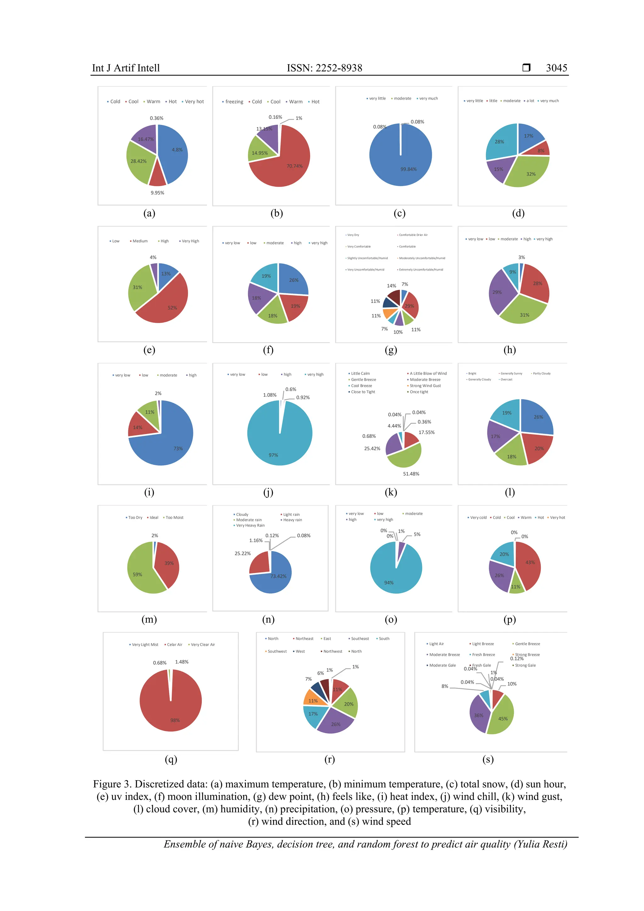
Figure 3 shows the discretization result of each predictor variable in the Shanghai city air quality
data. The discretization is created based on each variable's characteristics and value range, as presented in
Table 1. The predictor variables indicating weather factors are given in Figures 3(a)-3(i), while indicating
atmospheric phenomena in Figures 3(j)-3(s). In Figure 3(a), the maximum temperature variable is discretized
into cold (0 ˚C-20.4 ˚C), cool (20.5-23.9 ˚C), warm (24-29.9 ˚C), hot (30-37.9 ˚C), and very hot (>38 ˚C).
Figure 3(b) shows minimum temperature variable is discretized into freezing (<-0,1 ˚C), cold
(0-20.4 ˚C), cool (20.5-23.9 ˚C), warm (24-29.9 ˚C), hot (30-37.9 ˚C), and very hot (>38 ˚C). Total snow, as
presented in Figure 3(c), is discretized into very little (0-0.33 mm), moderate (0.68-1.01 mm), and very much
(>1.36 mm). Figure 3(d) discretizes sun hour into very little (3.9-5.93 hour), little (5.94-8.07 hour), moderate
(8.08-10.21 hour), a lot (10.22-12.35 hour), and very much (>12.36 hour). UV index, as shown in
Figure 3(e), discretized the data into low (1-2.9 nm), medium (3-5.9 nm), high (6-7.9 nm), and very high
(8-10.9 nm). The variable of moon illumination in Figure 3(f) discretizes the data into very low (0-19.9 ˚C),
low (20-39.9 ˚C), moderate (40-59.9 ˚C), high (60-79.9 ˚C), and very high (>80 ˚C). Figure 3(g) presents
discretization of dew point variable into very dry (<-0.1 ˚C), comfortable dry air (0-9.9 ˚C), very comfortable
(10-12.9 ˚C), comfortable (13-15.9 ˚C), slightly uncomfortable (16-17.9 ˚C), moderately uncomfortable
(18-20.9 ˚C), very uncomfortable (21-23.9 ˚C), and extremely uncomfortable (>24 ˚C). In Figure 3(h) feels
like variable is discretized into very low (<1.7 ˚C), low (1.8-12.5 ˚C), moderate (12.6-23.3 ˚C), high
(23.4-34.1 ˚C), and very high (>34.2 ˚C). Figure 3(i) shows that the heat index variable is discretized into
very low (<26.6 ˚C), low (26.7-32.1 ˚C), moderate (32.2-39.3 ˚C), and high (>34.2 ˚C).
-1
-0.8
-0.6
-0.4
-0.2
0
0.2
0.4
0.6
0.8
1
x1
x2
x3
x4
x5
x6
x7
x8
x9
x10
x11
x12
x13
x14
x15
x16
x17
x18
x19
x1
x2
x3
x4
x5
x6
x7
x8
x9
x10
x11
x12
x13
x14
x15
x16
x17
x18
x19

3045
(a) (b) (c) (d)
(e) (f) (g) (h)
(i) (j) (k) (l)
(m) (n) (o) (p)
(q) (r) (s)
Figure 3. Discretized data: (a) maximum temperature, (b) minimum temperature, (c) total snow, (d) sun hour,
(e) uv index, (f) moon illumination, (g) dew point, (h) feels like, (i) heat index, (j) wind chill, (k) wind gust,
(l) cloud cover, (m) humidity, (n) precipitation, (o) pressure, (p) temperature, (q) visibility,
(r) wind direction, and (s) wind speed
4.8%
9.95%
28.42%
16.47%
0.36%
Cold Cool Warm Hot Very hot
1%
70.74%
14.95%
13.15%
0.16%
freezing Cold Cool Warm Hot
99.84%
0.08%
0.08%
very little moderate very much
17%
8%
32%
15%
28%
very little little moderate a lot very much
13%
52%
31%
4%
Low Medium High Very High
26%
19%
18%
18%
19%
very low low moderate high very high
7%
29%
11%
10%
7%
11%
11%
14%
Very Dry Comfortable Drier Air
Very Comfortable Comfortable
Slightly Uncomfortable/Humid Moderately Uncomfortable/Humid
Very Uncomfortable/Humid Extremely Uncomfortable/Humid
3%
28%
31%
29%
9%
very low low moderate high very high
73%
14%
11%
2%
very low low moderate high
1.08%
0.6%
0.92%
97%
very low low high very high
0.36%
17.55%
51.48%
25.42%
4.44%
0.68%
0.04% 0.04%
Little Calm A Little Blow of Wind
Gentle Breeze Moderate Breeze
Cool Breeze Strong Wind Gust
Close to Tight Once tight
26%
20%
18%
17%
19%
Bright Generally Sunny Partly Cloudy
Generally Cloudy Overcast
2%
39%
59%
Too Dry Ideal Too Moist
73.42%
25.22%
1.16%
0.12% 0.08%
Cloudy Light rain
Moderate rain Heavy rain
Very Heavy Rain
0%
0%
1%
5%
94%
very low low moderate
high very high
0%
43%
11%
26%
20%
0%
Very cold Cold Cool Warm Hot Very hot
1.48%
98%
0.68%
Very Light Mist Celar Air Very Clear Air
1%
11%
20%
26%
17%
11%
7%
6%
1%
North Northeast East Southeast South
Southwest West Northwest North
0.12%
10%
45%
36%
8%
1%
0.04%
0.04%
0.04%
Light Air Light Breeze Gentle Breeze
Moderate Breeze Fresh Breeze Strong Breeze
Moderate Gale Fresh Gale Strong Gale

 ISSN: 2252-8938
3046
Wind chill variable in Figure 3(j) is discretized into very low (<0.1˚C), low (0-0.33 ˚C), normal (0.34-
0.67 ˚C), high (0.68 -1.01 ˚C), and very high (>1.02 ˚C). Variable of wind gust in Figure 3(k) discretize the data
into little calm (1-5 km/h), a little blow (6-11 km/h), gentle breeze (12-19 km/h), moderate breeze (20-29 km/h),
and cool breeze (30-39 km/h). Figure 3(l) shows cloud cover variable is discretized into bright (0-20 octa),
generally sunny (21-40 octa), partly cloudy (41-60 octa), generally cloudy (61-80 octa), and overcast
(> 81 octa). Humidity variable, as presented in Figure 3(m), is discretized into too dry (0-39%), ideal (40-69%),
and too moist (> 70%). Figure 3(n) shows precipitation variable is discretized into cloudy (< 0 mm), light rain
(1-20 mm), moderate (21-50 mm), heavy rain (51-100 mm), and very heavy (> 101 mm). In Figure 3(o), the
pressure variable is discretized into very low (986-996.5 mb), low (996.6-998.73 mb), moderate
(998.74-1000.87 mb), high (1000.88-1003.01 MB), and very high (>1003.02 MB). Figure 3(p) shows optimum
temperature variable is discretized into very cold (<-0,1 ˚C), cold (0-20.4 ˚C), cool (20.5-23.9 ˚C), warm
(24-29.9 ˚C), hot (30-37.9 ˚C), and very hot (>38 ˚C). Visibility variable in Figure 3(q) is discretized into dense
fog (0.03-0.15 m), moderate fog (0.16-0.53 m), very light fog (0.54-1.07 m), light mist (1.08-2.15 m), and very
light misc (2.16-5.3 m). Variable of wind direction degree in Figure 3(r) discretizes the data into north (0-23˚),
north east (24-68˚), east (69-113˚), south east (114-158˚), south (159-203˚), south west (204-248˚), west
(249-293˚), north west (294-336˚), and north (>337˚). Figure 3(s) shows wind speed variable is discretized into
light air (1-3 km/h), light breeze (4-7 km/h), gentle breeze (8-12 km/h), moderate breeze (13-18 km/h), fresh
breeze (19-24 km/h), strong breeze (25-31 km/h), moderate gale (32-38 km/h), and fresh gale (39-46 km/h).
The discretization result does not produce a balanced distribution of observations in each category
on each predictor variable. The distribution imbalance of each extreme category due to discretization based
on the characteristics of this variable can be found in the variables total snow (𝑋3), heat index (𝑋9), wind chill
(𝑋10), pressure (𝑋15), and visibility (𝑋17). However, the imbalance in the distribution of each category on
these predictor variables does not affect the significance of the response variable.
Furthermore, this study proposes the chi-squared test to determine the effect of discretized predictor
variables on the target variable. Table 3 shows the results of the chi-squared test where the two predictor variables,
total snow (𝑋3) and moon illumination (𝑋6) do not affect the target variable. In the next stage of the prediction
process, the existence of these two variables has a different effect on the performance of each prediction model.
Table 3. Chi-square test
Variable Chi-square df p-value
Maximum temperature (𝑋1) 10008.00 16 0.00
Minimum temperature (𝑋2) 3227.40 16 0.00
Total snow (𝑋3) 4.94 8 0.76
Sun hour (𝑋4) 1148.08 16 2.06 x 10-234
UV index (𝑋5) 2221.82 12 0.00
Moon illumination (𝑋6) 24.34 16 0.08
Dew point (𝑋7) 3168.70 28 0.00
Feels like (𝑋8) 3270.11 16 0.00
Heat index (𝑋9) 2745.12 12 0.00
Wind chill (𝑋10) 107.08 12 2.26 x 10-17
Wind gust (𝑋11) 146.12 24 1.73 x 10-19
Cloud cover (𝑋12) 199.83 16 8.60 x 10-34
Humidity (𝑋13) 135.46 8 2.08 x 10-25
Precipitation (𝑋14) 23.34 8 2.95 x 10-03
Pressure (𝑋15) 308.78 16 3.86 x 10-56
Temperature (𝑋16) 10008 16 0.00
Visibility (𝑋17) 12.56 4 0.01
Wind dir degree (𝑋18) 300.09 32 2.56 x 10-45
Wind speed (𝑋19) 95.60 28 2.58 x 10-09
3.2. Prediction of the air quality
Air quality for Shanghai data is predicted into five classes: hazardous, very unhealthy, unhealthy,
unhealthy for sensitive groups, and moderate. The prediction results are evaluated based on the confusion
matrix for multiclass problems using four metrics, namely accuracy, precision, recall, and F1-score [43],
[44]. NB, DT, and RF are implemented into two models for each single method. The first model includes all
predictor variables, and the second only involves significant variables based on the chi-square test. The
performance of the two models for each single method is presented in Table 4.
In the NB method, the prediction model's performance involving only significant variables increases
compared to the model involving all variables. The increase occurred in all four metrics as measured by
different percentages. However, it is inversely proportional to the DT and RF methods, where the prediction

3047
model's performance involving only significant variables is not higher than the model involving all variables,
also on the four metrics measured with different percentages. From the six models presented in Table 4, it
can be seen that the RF method with a model involving all variables is the model with the best performance
compared to the other five models. This fact shows that in this case, although the performance of the NB
model involving significant variables is not better than the DT and RF models, including only significant
variables in the prediction can improve the performance of the NB method. The four proposed models using
the supervised single methods have good accuracy (except two models of NB), more than 85% [45], but the
other three performance metrics are below 85%.
Table 4. The prediction performance of single methods
Metric Performance of proposed model (%)
NB DT RF
All variable Significant variable All variable Significant variable All variable Significant variable
Accuracy 78.02 78.23 99.05 96.91 99.15 97.39
Precision 27.30 31.10 78.59 72.22 78.20 74.66
Recall 32.97 33.15 77.46 74.66 78.34 74.04
F1-score 29.87 32.09 78.02 73.42 78.27 74.35
Furthermore, the performance of the ensemble model for both models is presented in Table 5. The
performance of each ensemble method is better than the single methods, but the other three performance
metrics are still below 85%. Ensemble methods that involve all variables in a single method that supports it
have better performance than those with only significant variables. This event naturally occurs because two
of the three single methods that support the ensemble method with models involving all variables perform
better than models involving only significant variables. The performance of a single model that supports the
ensemble method dramatically influences the performance of the ensemble model.
Table 5. The prediction performance of the ensemble method
Metric Performance of proposed model (%)
All variable Significant variable
Accuracy 99.89 97.51
Precision 79.60 74.58
Recall 79.81 74.44
F1-score 79.70 74.51
3.3. Performance comparison
Comparison with other research is presented in Tables 6 to 9, which each presents the performance
of three single and ensemble methods. In general, the NB implementation in various cases has good
performance metrics, especially accuracy, but the precision value is not always directly proportional to the
accuracy value. Good NB model performance is usually obtained because each category spreads the predictor
variable discretization evenly. Compared with the performance of the NB prediction method in Table 4,
which predicts air quality in the proposed model, with the performance of the NB method in Table 6, the
performance of the NB in Table 4 is unsatisfactory, especially on precision, recall, and F1 score metrics. The
possible cause is discretization, that is formed unevenly in each category. There are even categories with no
observations, thus affecting the probability calculation for each class. Other discretization techniques are
needed to get better NB performance. Even discretization in each category in a variable in each class allows
for good model performance, as achieved by previous researchers.
Table 6. The performance comparing of the NB
Research (dataset) Performance metric (%)
Accuracy Precision Recall
Kaushik et al. [15] (customer sentiment) 94.00 93.00 94.00
Resti et al. [16] (corn plant disease and pest) 97.72 79.88 79.24
Safarkhani and Moro [17] (bank depositor's behavior) 90.82 - 96.10
Resti et al. [18] (diabetes mellitus disease) 95.83 93.82 94.48
Agghey et al. [20] (username enumeration attack) 95.70 94.85 -
Akbar et al. [21] (android malware) 89.52 89.53 89.52

 ISSN: 2252-8938
3048
Table 7. The performance comparing of DT
Resti et al. [46] (corn plant disease and pest) 94.53 84.31 83.07
Eliyati et al. [19] (air quality of Shanghai) 99.05 78.59 77.46
Panigrahi et al. [24] (maize leaf disease) 74.35 73.00 74.00
Table 8. The performance comparing RF
Akbar et al. [21] (android malware) 89.96 89.97 89.96
Musaddiq et al. [23] (student's performance) 88.80 89.00 88.00
Singh et al. [22] (rice plant leaf disease) 100.00 100.00 100.00
Nurhachita and Negara [25] (admission of the new student) 44.65 - -
Table 9. Performance comparison of the ensemble method is higher than the single method
Research (dataset) Ensemble of methods Accuracy
Gaurav et al. [37] (chronic kidney disease) SVM, C45, PSO-MLP, DT 92.76
Tinh and Mai [31] (indoor WIFI positioning) RF, KNN, DNN 98.90
Elmahalwy et al. [35] (KDD Cup-99) Isolation Forest & IForest-KMeans 99.70
Elmahalwy et al. [35] (credit card) 97.54
Elmahalwy et al. [35] (WPBC) 97.07
Elmahalwy et al. [35] (forest cover) 94.00
Elmahalwy et al. [35] (Pima) 94.24
Awotunde et al. [36] (IIOT networks of fridge sensor) RF, Extra Tree, AdaBoost, Bagging 98.73
Awotunde et al. [36] (IIOT networks of the thermostat) 98.83
Awotunde et al. [36] (IIOT networks of GPS tracker) 98.69
Awotunde et al. [36] (IIOT networks of Modbus) 99.13
As with NB, in general, the implementation of DT in various cases as shown in Table 7 has good
performance metrics, especially accuracy. However, the precision and recall values are sometimes not
directly proportional to the accuracy values. The performance of the DT method in predicting air quality in
the proposed models provided very satisfactory performance (accuracy) (more than 96%) in both models in
Table 4. This fact indicates that the DT method does not require data normalization, considering that the DT
method is nonparametric. In addition, the DT method is more resistant to the distribution of observations that
are not evenly distributed in each class.
Rarely does RF implementation in various cases have poor performance metrics, but this does not
mean such cases do not exist as shown in Table 8. The RF implementation on the admission of the new
student shows an accuracy performance of less than 45% [25]. However, like the other two methods, the
precision and recall values are not always directly proportional to the accuracy values. Generally, this event
occurs in multiclass cases with unequal class proportions. Other experiments are needed to improve these two
metrics, for example, by resampling techniques [13], [46]. Compared with the prediction performance of air
quality in the proposed single methods, the RF is the best method in both models, with all variables and the
significant variables only. The proposed RF has good accuracy, most above 97%.
Table 9 presents the performance of the ensemble method in some datasets. In the chronic kidney
disease (CKD) dataset, the performance of the ensemble method, especially the accuracy, has increased
compared to the accuracy of all single methods. The accuracy of the single method for the CKD dataset from
lowest to highest is 64.5% SVM, 72.67% DT, 75.32% C4.5, and 86.31% particle swarm optimization-
multilayer perceptron (PSO-MLP). In this case, the accuracy increased significantly compared to the single
method, around 6.45% - 28.26%. Likewise, for the indoor WIFI positioning dataset, bank bankruptcy, KDD
Cup-99, credit card, WPBC, forest cover, Pima datasets, fridge sensor, thermostat, GPS tracker, and Modbus
datasets. For the indoor Wifi positioning dataset [31], the accuracy of the single method from lowest to
highest is 98.35 k-nearest neighbor (KNN), 98.5% RF, and 98.7% deep neural networks (DNN). The three
proposed methods have good accuracy (more than 98%), but the ensemble method has a higher accuracy.
The majority of IForest-Kmeans accuracy is higher than isolation forest. The increase in the ensemble
method ranges from 2.23% (KDD cup-99 dataset) to 33.43% (credit card dataset) [35]. In the intrusion of
IIoT datasets [36], only the Adaboost method has low accuracy. The other three methods have accuracy that
competes with the proposed ensemble method. Accuracy for networks of fridge sensor, thermostat, GPS
tracker, and Modbus are 98.43%, 98.65%, 98.13%, 98.78% (RF), 98.01%, 98.38%, 97.66%, 98.78% (extra

3049
tree ET)), 48.09% respectively, 53.05%, 47.38%, 62.92% (AdaBoost), and 98.56%, 98.58%, 98.32%,
98.90% (Bagging). Globally, the increase in the ensemble method ranges from 0.35% (Modbus dataset) to
51.31% (GPS tracker).
4. CONCLUSION
This study predicts the air quality of Shanghai using the ensemble method. The method is built
based on single methods consisting of NB, DT, and RF methods. Two models are proposed for each single
and ensemble method. The conclusion of this study consists of two points. First, selecting significant
predictor variables on the response variable using the chi-square test positively impacts the performance of
the NB method, but not so with the other two single methods, DT, and RF. Second, the ensemble method has
succeeded in improving the performance of a single method in both models, involving all variables and only
significant variables. However, the performance of the ensemble method for models involving all variables is
better on the four performance-metrics for multiclass. The best prediction results indicated by the model's
performance with the highest metric are expected to be a reference in carrying out prediction tasks. In
addition, it is hoped that it will be helpful for the government and the community to take policies and actions
to reduce/avoid the adverse effects of air quality.
ACKNOWLEDGEMENTS
The authors thank the University of Sriwijaya for funding Science and Technology Research no.
0165.025/ UN9/ SB3.LP2M. PT/2022, June 22nd, 2022.
REFERENCES
[1] Y. Yan, Y. Li, M. Sun, and Z. Wu, “Primary pollutants and air quality analysis for urban air in china: evidence from Shanghai,”
Sustainability, vol. 11, no. 8, Apr. 2019, doi: 10.3390/su11082319.
[2] S. Zeng and Y. Zhang, “The effect of meteorological elements on continuing heavy air pollution: a case study in the chengdu area
during the 2014 spring festival,” Atmosphere, vol. 8, no. 4, Apr. 2017, doi: 10.3390/atmos8040071.
[3] J. Cai, X. Dai, L. Hong, Z. Gao, and Z. Qiu, “An air quality prediction model based on a noise reduction self-coding deep
network,” Mathematical Problems in Engineering, vol. 2020, pp. 1–12, May 2020, doi: 10.1155/2020/3507197.
[4] M. Jia et al., “Regional air quality forecast using a machine learning method and the WRF model over the yangtze river delta, east
China,” Aerosol and Air Quality Research, vol. 19, no. 7, pp. 1602–1613, 2019, doi: 10.4209/aaqr.2019.05.0275.
[5] P. Mannucci and M. Franchini, “Health effects of ambient air pollution in developing countries,” International Journal of
Environmental Research and Public Health, vol. 14, no. 9, Sep. 2017, doi: 10.3390/ijerph14091048.
[6] Y. Pan, H. Gao, H. Lin, Z. Liu, L. Tang, and S. Li, “Identification of bacteriophage virion proteins using multinomial naïve Bayes
with g-gap feature tree,” International Journal of Molecular Sciences, vol. 19, no. 6, Jun. 2018, doi: 10.3390/ijms19061779.
[7] J. Dougherty, R. Kohavi, and M. Sahami, “Supervised and unsupervised discretization of continuous features,” Proceedings of the
12th International Conference on Machine Learning, ICML 1995, pp. 194–202, 1995, doi: 10.1016/b978-1-55860-377-6.50032-3.
[8] S. García, J. Luengo, and F. Herrera, “Data preprocessing in data mining,” Intelligent Systems Reference Library, Cham:
Springer, vol. 72, 2015.
[9] Q. Chen and M. Huang, “Rough fuzzy model-based feature discretization in intelligent data preprocess,” Journal of Cloud
Computing, vol. 10, no. 1, Dec. 2021, doi: 10.1186/s13677-020-00216-4.
[10] A. Podviezko and V. Podvezko, “Influence of data transformation on multicriteria evaluation result,” Procedia Engineering, vol.
122, pp. 151–157, 2015, doi: 10.1016/j.proeng.2015.10.019.
[11] M. Kuhn and K. Johnson, Applied predictive modeling. New York: Springer, 2013, doi: 10.1007/978-1-4614-6849-3.
[12] Y. Resti, C. Irsan, A. Neardiaty, C. Annabila, and I. Yani, “Fuzzy discretization on the multinomial naïve bayes method for
modeling multiclass classification of corn plant diseases and pests,” Mathematics, vol. 11, no. 8, Apr. 2023, doi:
10.3390/math11081761.
[13] A. Altay and D. Cinar, “Fuzzy decision trees,” Fuzzy Statistical Decision-Making, 2016, pp. 221–261. doi: 10.1007/978-3-319-
39014-7_13.
[14] I. H. Witten, E. Frank, and M. A. Hall, Data mining: practical machine learning tools and techniques, Burlington, USA: Elsevier,
2011.
[15] K. Kaushik et al., “Multinomial naive bayesian classifier framework for systematic analysis of smart IoT devices,” Sensors, vol.
22, no. 19, Sep. 2022, doi: 10.3390/s22197318.
[16] Y. Resti, C. Irsan, M. T. Putri, I. Yani, Anshori, and B. Suprihatin, “Identification of corn plant diseases and pests based on digital
images using multinomial naïve bayes and k-nearest neighbor,” Science and Technology Indonesia, vol. 7, no. 1, pp. 29–35, 2022,
doi: 10.26554/sti.2022.7.1.29-35.
[17] F. Safarkhani and S. Moro, “Improving the accuracy of predicting bank depositor’s behavior using a decision tree,” Applied
Sciences, vol. 11, no. 19, Sep. 2021, doi: 10.3390/app11199016.
[18] Y. Resti, E. S. Kresnawati, N. R. Dewi, D. A. Zayanti, and N. Eliyati, “Diagnosis of diabetes mellitus in women of reproductive
age using the prediction methods of naive Bayes, discriminant analysis, and logistic regression,” Science and Technology
Indonesia, vol. 6, no. 2, pp. 96–104, Apr. 2021, doi: 10.26554/STI.2021.6.2.96-104.
[19] N. Eliyati, M. Rahmayani, S. Wijaya, D. A. Zayanti, E. S. Kresnawati, and Y. Resti, “Prediction of air quality index using
decision tree with discretization,” Indonesian Journal of Engineering and Science, vol. 3, no. 3, pp. 61–67, Nov. 2022, doi:
10.51630/ijes.v3i3.82.
[20] A. Z. Agghey, L. J. Mwinuka, S. M. Pandhare, M. A. Dida, and J. D. Ndibwile, “Detection of username enumeration attack on ssh
protocol: Machine learning approach,” Symmetry, vol. 13, no. 11, Nov. 2021, doi: 10.3390/sym13112192.

 ISSN: 2252-8938
3050
[21] F. Akbar, M. Hussain, R. Mumtaz, Q. Riaz, A. W. A. Wahab, and K.-H. Jung, “Permissions-based detection of android malware
using machine learning,” Symmetry, vol. 14, no. 4, Apr. 2022, doi: 10.3390/sym14040718.
[22] A. K. Singh, B. Chourasia, N. Raghuwanshi, and R. K, “BPSO based feature selection for rice plant leaf disease detection with
random forest classifier,” International Journal of Engineering Trends and Technology, vol. 69, no. 4, pp. 34–43, Apr. 2021, doi:
10.14445/22315381/IJETT-V69I4P206.
[23] M. H. Musaddiq, M. S. Sarfraz, N. Shafi, R. Maqsood, A. Azam, and M. Ahmad, “Predicting the impact of academic key factors
and spatial behaviors on students’ performance,” Applied Sciences, vol. 12, no. 19, Oct. 2022, doi: 10.3390/app121910112.
[24] K. P. Panigrahi, H. Das, A. K. Sahoo, and S. C. Moharana, “Maize leaf disease detection and classification using machine
learning algorithms,” Progress in Computing, Analytics and Networking: Proceedings of ICCAN 2019, 2020, pp. 659–669. doi:
10.1007/978-981-15-2414-1_66.
[25] N. Nurhachita and E. S. Negara, “A comparison between deep learning, naïve Bayes and random forest for the application of data
mining on the admission of new students,” IAES International Journal of Artificial Intelligence (IJ-AI), vol. 10, no. 2, Jun. 2021,
doi: 10.11591/ijai.v10.i2.pp324-331.
[26] I. E. Livieris, A. Kanavos, V. Tampakas, and P. Pintelas, “A weighted voting ensemble self-labeled algorithm for the detection of
lung abnormalities from X-rays,” Algorithms, vol. 12, no. 3, Mar. 2019, doi: 10.3390/A12030064.
[27] S. Karlos, G. Kostopoulos, and S. Kotsiantis, “a soft-voting ensemble based co-training scheme using static selection for binary
classification problems,” Algorithms, vol. 13, no. 1, Jan. 2020, doi: 10.3390/a13010026.
[28] S. Dutt, S. Chandramouli, and A. K. Das, Machine learning. India: Pearson India Education Service Pvt. Ltd, 2016.
[29] P. Pintelas and I. E. Livieris, “Special issue on ensemble learning and applications,” Algorithms, vol. 13, no. 6, Jun. 2020, doi:
10.3390/A13060140.
[30] R. Matteo and V. Giorgio, “Ensemble methods: a review,” Data Mining and Machine Learning for Astronomical Applications,
pp. 3–40, 2012.
[31] D. T. Pham and T. T. N. Mai, “Ensemble learning model for Wifi indoor positioning systems,” IAES International Journal of
Artificial Intelligence (IJ-AI), vol. 10, no. 1, p. 200, Mar. 2021, doi: 10.11591/ijai.v10.i1.pp200-206.
[32] Z. H. Zhou, Ensemble methods: foundations and algorithms, Boca Raton, Florida: Chapman & Hall/CRC, 2012, doi:
10.1201/b12207.
[33] J. Ha, M. Kambe, and J. Pe, Data mining: concepts and techniques. Morgan Kaufmann, 2011. doi: 10.1016/C2009-0-61819-5.
[34] C. Zhang and Y. Ma, Ensemble machine learning: methods and applications, New York: Springer Publishing, 2012, doi:
10.1007/9781441993267.
[35] A. M. Elmahalwy, H. M. Mousa, and K. M. Amin, “New hybrid ensemble method for anomaly detection in data science,”
International Journal of Electrical and Computer Engineering (IJECE), vol. 13, no. 3, pp. 3498-3508, Jun. 2023, doi:
10.11591/ijecev13i3.pp3498-3508.
[36] J. B. Awotunde, C. Chakraborty, and A. E. Adeniyi, “Intrusion detection in industrial internet of things network-based on deep
learning model with rule-based feature selection,” Wireless Communications and Mobile Computing, vol. 2021, pp. 1–17, Sep.
2021, doi: 10.1155/2021/7154587.
[37] K. Gaurav, D. A. Naik, V. K. Jaiswal, A. M, and A. V, “Chronic kidney disease prediction,” International Journal of Computer
Sciences and Engineering, vol. 7, no. 4, pp. 1065–1069, Apr. 2019, doi: 10.26438/ijcse/v7i4.10651069.
[38] M. Shanmugapriya, H. K. Nehemiah, R. S. Bhuvaneswaran, K. Arputharaj, and J. D. Sweetlin, “Fuzzy discretization based
classification of medical data,” Research Journal of Applied Sciences, Engineering and Technology, vol. 14, no. 8, pp. 291–298,
Aug. 2017, doi: 10.19026/rjaset.14.4953.
[39] N. M. Razali and Y. B. Wah, “Power comparisons of shapiro-wilk, kolmogorov-smirnov, lilliefors and anderson-darling tests,”
Journal of Statistical Modeling and Analytics, vol. 2, no. 1, pp. 13–14, 2011.
[40] G. J. Székely and M. L. Rizzo, “A new test for multivariate normality,” Journal of Multivariate Analysis, vol. 93, no. 1, pp. 58–
80, Mar. 2005, doi: 10.1016/j.jmva.2003.12.002.
[41] D. Conn, T. Ngun, G. Li, and C. M. Ramirez, “Fuzzy forests: extending random forest feature selection for correlated, high-
dimensional data,” Journal of Statistical Software, vol. 91, no. 9, 2019, doi: 10.18637/jss.v091.i09.
[42] M. Hallin and D. Paindaveine, “Optimal tests for homogeneity of covariance, scale, and shape,” Journal of Multivariate Analysis,
vol. 100, no. 3, pp. 422–444, Mar. 2009, doi: 10.1016/j.jmva.2008.05.010.
[43] S. Dinesh and T. Dash, “Reliable evaluation of neural network for multiclass classification of real-world data,” Arxiv-Computer
Science, pp. 1-6, Nov. 2016.
[44] M. Sokolova and G. Lapalme, “A systematic analysis of performance measures for classification tasks,” Information Processing
& Management, vol. 45, no. 4, pp. 427–437, Jul. 2009, doi: 10.1016/j.ipm.2009.03.002.
[45] S. Aronoff, “Classification accuracy: a user approach.,” Photogrammetric Engineering and Remote Sensing, vol. 48, no. 8, pp.
1299–1307, 1982.
[46] Y. Resti, C. Irsan, M. Amini, I. Yani, R. Passarella, and D. A. Zayantii, “Performance improvement of decision tree model using
fuzzy membership function for classification of corn plant diseases and pests,” Science and Technology Indonesia, vol. 7, no. 3,
pp. 284–290, Jul. 2022, doi: 10.26554/sti.2022.7.3.284-290.
BIOGRAPHIES OF AUTHORS
Yulia Resti holds a Doctor of Statistics degree from the National University of
Malaysia, Malaysia in 2013. She received her B.Sc. in Mathematics in 1996 and her M.Sc. in
Actuarial Science in 2003. Each from the University of Sriwijaya and Bandung Institute of
Technology, Indonesia. She is a member of the Indonesian Mathematical Society (Indoms),
and is now the governor of Indoms. She is currently a professor in the field of Statistics at the
Department of Mathematics at the University of Sriwijaya, Indonesia. Her research includes
statistical machine learning, data mining, applied statistics, and actuarial science. She can be
contacted at email: yulia_resti@mipa.unsri.ac.id.

3051
Ning Eliyati received her B.Sc. (Mathematics) from the University of Padjajaran,
Indonesia, and her M.Ed. (Mathematics Education) from the University of Sriwijaya,
Indonesia. She is a lecturer at the Department of Mathematics, University of Sriwijaya,
Indonesia. Her research includes applied statistics, optimization, statistical machine learning,
data mining, and actuarial science. She is a member of the Indonesian Mathematical Society
(Indoms). She can be contacted at email: ning_eliyati @mipa.unsri.ac.id.
Mauizzatil Rahmayanti a student in the Mathematics Department, Faculty of
Mathematics and Natural Science, University of Sriwijaya, Indonesia. She can be contacted at
email: 08011281823038@student.unsri.ac.id or rahmayani557@gmail.com.
Des Alwine Zayanti obtained a B.Sc. (Mathematics) from the University of
Sriwijaya, Indonesia, in 1994. Her M.Sc. is from Actuarial Science at Bandung Institute of
Technology, Indonesia. She currently teaches at the Department of Mathematics at Sriwijaya
University, Indonesia. She is a member of the Indonesian Mathematical Society (Indoms). Her
research includes applied statistics, optimization, statistical machine learning, data mining, and
actuarial science. She can be contacted at desalwinez@unsri.ac.id.
Endang Sri Kresnawati has degrees in both Mathematics and Actuarial Science
from Indonesia's Bandung Institute of Technology and University of Sriwijaya, respectively.
She is a lecturer at the Indonesian University of Sriwijaya's Department of Mathematics. She
is enrolled in a doctoral program at Sriwijaya University in Indonesia with a mathematics
concentration. She belongs to both Indoms and the Indonesian Mathematical Society. She
conducts research in data mining, statistical machine learning, applied statistics, and actuarial
science. She can be contacted at email: eskresna@unsri.ac.id.
Endro Setyo Cahyono earned his M.Sc. (Mathematics) from Bandung Institute
of Technology in Indonesia in 1998 after earning his B.Sc. (Mathematics) from November
10th Institute of Technology in Surabaya, Indonesia, in 1988. He is currently giving lectures at
the Indonesian University of Sriwijaya's Department of Mathematics. He is an Associate
Professor at Department of Mathematics at the University of Sriwijaya, Indonesia. His work
involves applied statistics and mathematics. He can be contacted at email:
endrosetyocahyono@mipa.unsri.ac.id.
Irsyadi Yani is an Associate Professor in the Department of Mechanical
Engineering, Faculty of Engineering at the University of Sriwijaya, where he has been a
faculty member since 1997. He received a B.Eng. degree in Mechanical Engineering from the
University of Sriwijaya, Indonesia, and M.Eng. degree in Mechanical Engineering from
Toyohashi University of Technology, Japan. He completed his Ph.D. at Universiti
Kebangsaaan Malaysia (UKM). His research interests lie in artificial intelligence, automatic
sorting systems, and machine learning. He has collaborated actively with researchers in
several other disciplines of Engineering and Science. He can be contacted at email: irsyadiyani
@ft.unsri.ac.id.

Ensemble of naive Bayes, decision tree, and random forest to predict air quality

More Related Content

Similar to Ensemble of naive Bayes, decision tree, and random forest to predict air quality

More from IAESIJAI

Recently uploaded

Ensemble of naive Bayes, decision tree, and random forest to predict air quality