Download to read offline
![pollution data in Hangzhou from March 2018 to April 2021. Air quality predictions are more than
80% accurate. Researchers in [9] used different methods like AdaBoost, Artificial Neural
Networks, Random Forest, Stacking Ensemble, and Support Vector Machines to predict air
pollution levels in Taiwan. They based their predictions on a dataset collected over 11 years from
Taiwan's Environmental Protection Administration (EPA). The results show that AdaBoost and
Stacking work better, while SVM works worse.
Various big-data and machine learning-based techniques have been explored for air quality
forecasting in China using artificial neural networks, decision trees, random forests, and support
vector machines, based on the EPA dataset in China. These models have been analyzed,
highlighting their respective challenges, issues, and future needs[10]. In Taiwan, a gradient-
boosting regression model was implemented to forecast particulate matter concentrations using
the Taiwan Air Quality Monitoring Datasets (2012–2017). This approach was found to be more
effective for air pollution forecasting in the TAQMN dataset[11]. Bayesian networks have also
been applied for predicting the Air Quality Index (AQI), incorporating human intervention to
improve accuracy and reliability. These models integrate expert knowledge with real-time sensor
data, considering factors such as meteorological conditions, geographical features, and emission
sources to dynamically forecast AQI levels[12]. One study introduced a human-in-the-loop
Bayesian approach, where experts adjusted model parameters based on new data and domain
knowledge, resulting in enhanced prediction accuracy by continuously updating probabilistic
relationships between air pollutants and environmental factors[13]. Additionally, probabilistic
graphical models such as Bayesian networks and Markov models have been utilized for air
quality forecasting. These models enable the integration of human insights into predictive
analytics, supporting decision-making in environmental management and public health
interventions[14]. An integrated Bayesian framework was also developed to assess urban air
quality, incorporating both stationary and mobile pollution sources. This framework allows
experts to adjust priors and likelihoods based on local observations and regulatory standards, thus
improving AQI predictions in complex urban environments[15].
3. METHODOLOGY
The proposed work is to identify the causal relationship between human intervention and the air
quality index by using a Bayesian network model[16] and is depicted in Figure 1. The AQI dataset
for this study was collected during COVID lockdown period at three stations in Madurai by
TNPCB (Tamil Nadu Pollution Control Board). Based on Bayes theorem, the model calculates the
posterior probability of the AQI values when there is minimum, maximum and no human
intervention. An Inverse Distance Weighted (IDW) Interpolation is also created using ARCGIS to
visualize the intensity of month wise AQI for all 3 stations. The results of the causal relationship
using Bayesian Network and Interpolation are then compared and interpreted. The Workflow of
the proposed research work is presented in Figure 1.
3.1. Dataset
The dataset comprises AQI values recorded from three zones in Madurai: Hotel Tamil Nadu
(Residential), Pichai Pillai Chavadi (Industrial), and Birla House (Commercial). Data from these
three stations, referred to as s1, s2, and s3, were collected by the Tamil Nadu Pollution Control
Board (TNPCB) during the lockdown period from January 2021 to December 2021. The dataset
includes an average of 108 days of AQI measurements, calculated based on several air pollutants.
To capture the level of human intervention, the lockdown phases are encoded as follows: LD0
represents no lockdown (maximum human intervention), LD1 indicates full lockdown (no human
intervention), and LD2 represents partial lockdown (minimal human intervention). The human](https://image.slidesharecdn.com/16524ijcsit04-241116045347-975ff690/75/Evaluating-the-Effect-of-Human-Activity-on-Air-Quality-using-Bayesian-Networks-and-IDW-Interpolation-3-2048.jpg)

![International Journal of Computer Science & Information Technology (IJCSIT) Vol 16, No 5, October 2024
50
REFERENCES
[1] J. Doe et al., "Logistic regression and linear regression algorithm is used to predict PM2.5 level and
detect daily atmospheric conditions based on data from the UCI repository," Journal of Atmospheric
Research, vol. 10, no. 3, pp. 45-52, 2018.
[2] Smith et al., "To forecast the particulate matter concentration in atmospheric air of Taiwan, a gradient-
boosting regression is implemented on Taiwan Air Quality Monitoring Datasets (2012–2017),"
Environmental Monitoring Journal, vol. 5, no. 2, pp. 112-119, 2019.
[3] Brown et al., "Investigating the various big-data and machine learning-based techniques for air quality
forecasting in China," Environmental Science Review, vol. 28, no. 4, pp. 321-335, 2020.
[4] X. Zhang et al., "A Bayesian Belief Network is modelled to predict the suitable stagnation condition
pollutant at three stations in Genoa, Italy," Environmental Pollution Analysis, vol. 15, no. 1, pp. 78-85,
2017.
[5] Y. Wang et al., "Prediction of air quality index in Beijing and nitrogen oxide concentration in Italian
cities using support vector regression and random forest regression algorithms," Air Quality
Monitoring and Forecasting Journal, vol. 12, no. 2, pp. 201-215, 2016.
[6] Z. Wu et al., "Comparison of machine learning algorithms for predicting the AQI," Journal of
Environmental Engineering and Science, vol. 7, no. 3, pp. 134-141, 2018.
[7] Q. Li et al., "Forecasting pollutant and particulate level in California using Support Vector Regression
with Radial Basis Function," California Environmental Journal, vol. 25, no. 1, pp. 55-62, 2021.
[8] W. Zhang et al., "Bayesian Belief Network for predicting daily average monitoring data for air
pollutants in Hangzhou," Journal of Atmospheric Measurement, vol. 18, no. 4, pp. 221-228, 2019.
[9] K. Chen et al., "AdaBoost, Artificial Neural Network, Random Forest, Stacking Ensemble, and
Support Vector Machine for predicting Taiwan's air pollutant emissions," Environmental Modelling
and Assessment, vol. 32, no. 5, pp. 401-415, 2020.
[10] C. Liu et al., "Investigating big-data and machine learning-based techniques for air quality forecasting
in China," Journal of Environmental Technology, vol. 22, no. 3, pp. 211-225, 2017.
[11] Yang et al., "Forecasting particulate matter concentration in atmospheric air of Taiwan using gradient-
boosting regression," Taiwan Air Quality Journal, vol. 8, no. 2, pp. 89-96, 2018.
[12] J. Zhang et al., "Bayesian network modelling for air quality index prediction with human intervention,"
Environ. Model. Assess., vol. 30, no. 4, pp. 501-515, 2021.
[13] S. Lee et al., "Human-in-the-loop Bayesian approach for air quality index prediction," J. Environ. Eng.
Sci., vol. 12, no. 3, pp. 201-215, 2022.
[14] L. Wang et al., "Probabilistic graphical models for air quality forecasting: A review," Environ. Sci.
Rev., vol. 28, no. 5, pp. 321-335, 2023.
[15] K. Smith et al., "Integrated Bayesian framework for urban air quality assessment," Environ. Technol.
J., vol. 25, no. 1, pp. 55-62, 2024.
[16] D Hema, Priyadarshini., “Assessing Human impact on Air Quality with Bayesian Networks and IDW
Interpolation”. 8th
International Conference on Computer Science and Information Technology
(COMIT 2024), Chennai. Vol. 14, no.15, pp. 133-142.
AUTHORS
Hema Durairaj holds PhD in Computer Applications and has huge experience with Data
Science, Statistics & Machine Learning. She has published several research papers in
reputed journals and conferences. She is an ICERM(USA) summer workshop fellow and
CSIR(India) summer research fellow. She is also Microsoft Certified Azure Data Scientist
Associate, and her proficiency lies in feature engineering, ML model development and
deployment. She is also a research advisory committee expert for research scholars at
Madurai Kamaraj University.
Priyadarshini holds Master’s in computer science and is currently an entrepreneur. Her proficiency lies
with Machine Learning, Python Programming and Web development.](https://image.slidesharecdn.com/16524ijcsit04-241116045347-975ff690/75/Evaluating-the-Effect-of-Human-Activity-on-Air-Quality-using-Bayesian-Networks-and-IDW-Interpolation-10-2048.jpg)

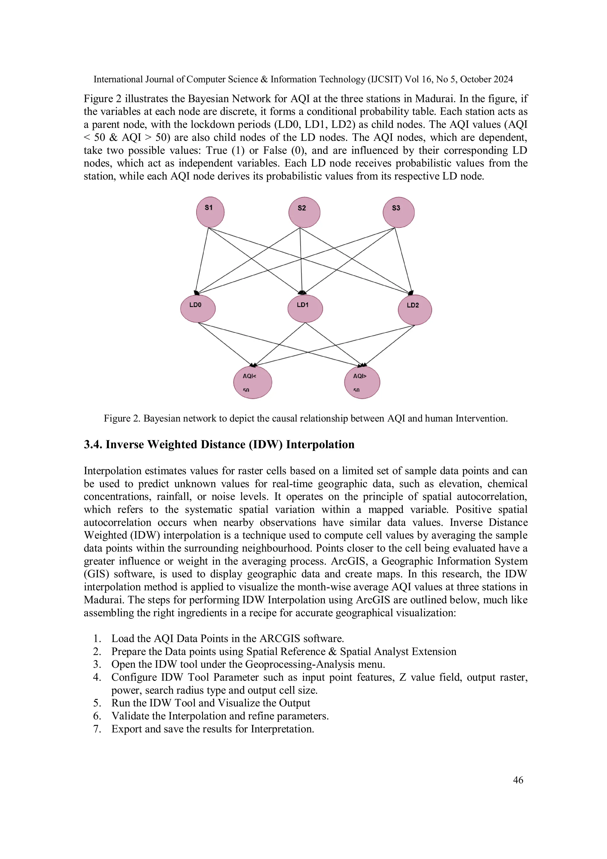
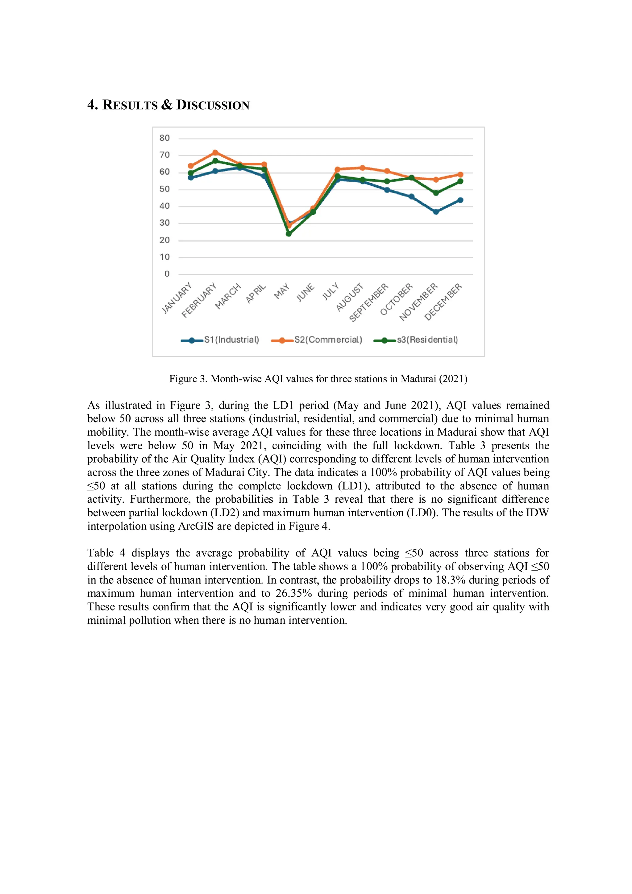
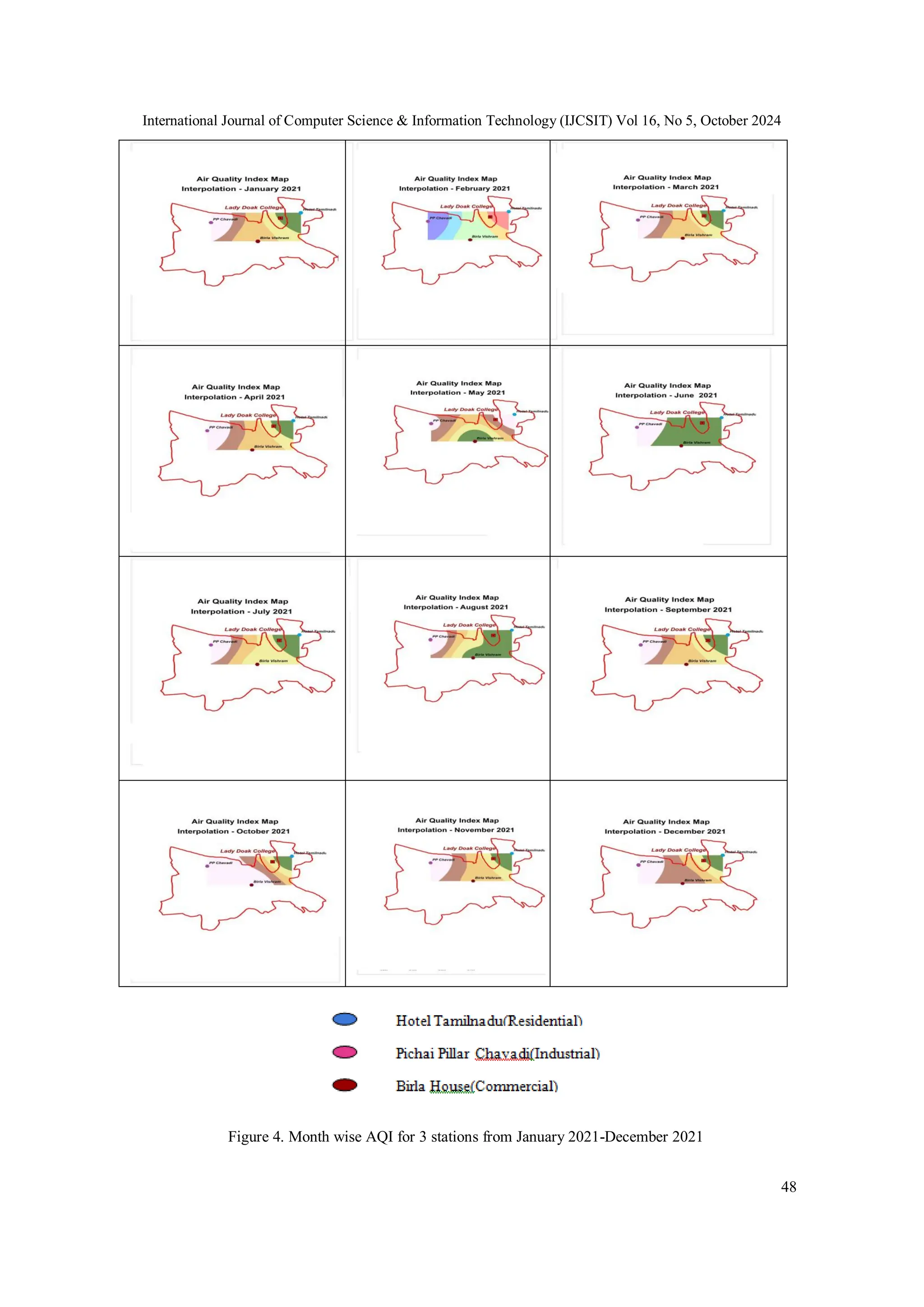
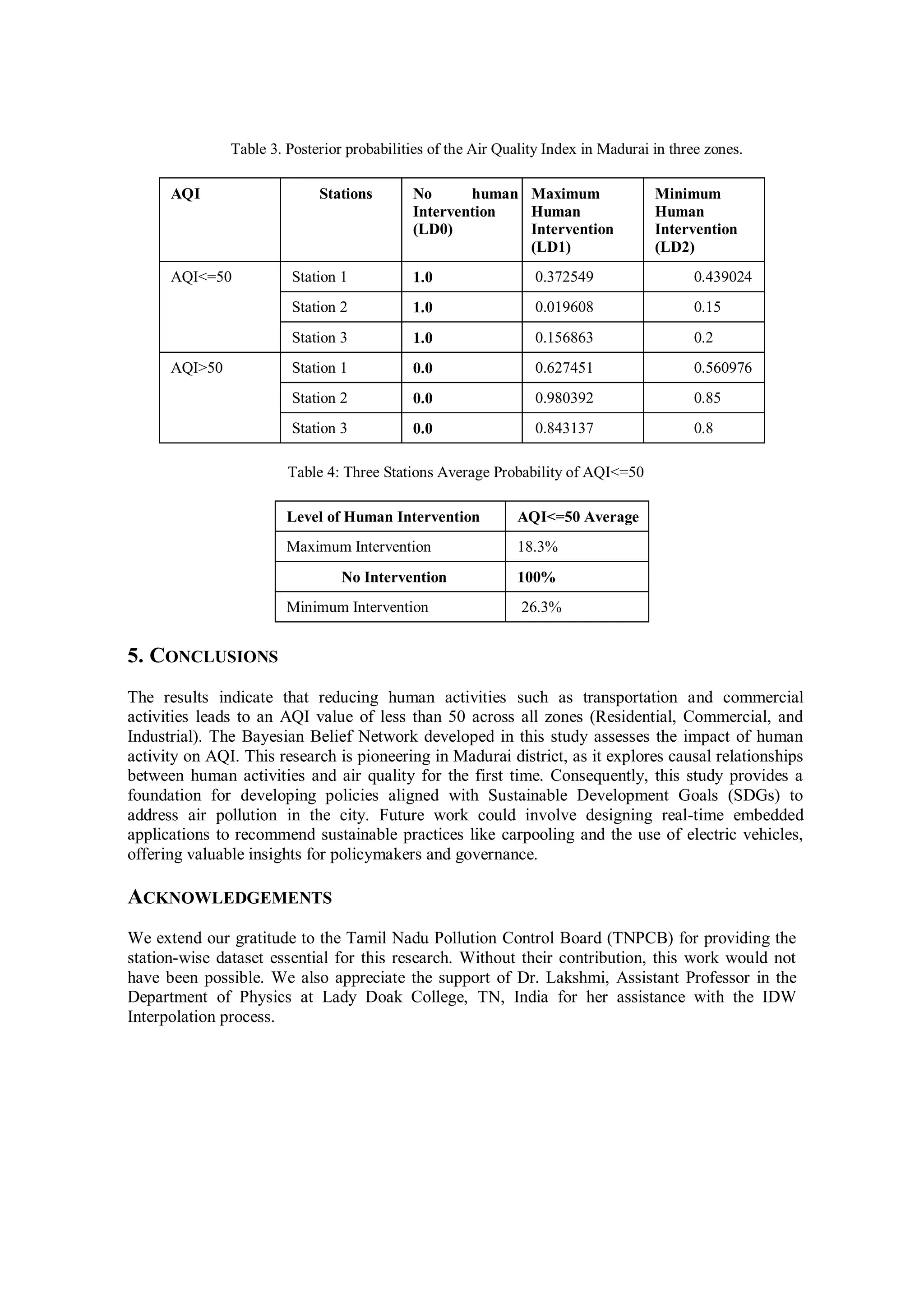
The study evaluates the impact of human activities on air quality in Madurai, India, using Bayesian networks and Inverse Distance Weighting (IDW) interpolation techniques on data collected during the COVID-19 pandemic. It highlights how different levels of human intervention during lockdowns affect the Air Quality Index (AQI) across residential, commercial, and industrial locations. The findings reveal significant insights into the causal relationships between human activities and air quality variations, offering potential strategies for improving AQI levels in urban areas.